The effect of polydispersity on the ordering transition of adsorbed self-assembled rigid rods

Abstract

Extensive Monte Carlo simulations were carried out to investigate the nature of the ordering transition of a model of adsorbed self-assembled rigid rods on the bonds of a square lattice [Tavares et. al., Phys. Rev E 79, 021505 (2009)]. The polydisperse rods undergo a continuous ordering transition that is found to be in the two-dimensional Ising universality class, as in models where the rods are monodisperse. This finding is in sharp contrast with the recent claim that equilibrium polydispersity changes the nature of the phase transition in this class of models [López et. al., Phys. Rev E 80, 040105(R)(2009)].

I Introduction

It has been shown, recently, that pure hard-rod models in two-dimensions (2D) exhibit discrete orientational order without translational order Ioffe , driven by a mechanism resembling that proposed by Onsager for the nematic transition of rods in three dimensions Onsager . Specifically, it was proved that a system of rods on the square lattice, with hard-core exclusion and length distribution between 2 and $n$, exhibits discrete orientational long-range order for suitable fugacities and large $n$. This may seem surprising as the nature of the transition of monodisperse freely rotating rods in 2D remains subtle, as it appears to depend on the details of the particle interactions Straley ; Frenkel ; Vink .

Simple 2D restricted orientation models are relevant to describe the sub-monolayer regime of linear molecules adsorbed on crystalline substrates Potoff and, even without polydispersity, rigid rod (RR) models were shown to exhibit a number of interesting featuresMatoz2008a ; Matoz2008b ; Ghosh . It was found that the ordered phase is stable for sufficiently large aspect ratiosMatoz2008a ; Ghosh and that the transition on the square lattice is 2D Ising Matoz2008b .

Polydisperse restricted orientation RR models are generalizations of the Zwanzig modelZwanzig , and provide a useful starting point for understanding the effects of polydispersity on the phase behavior of RRsClarke . The description of self-assembled rods has to consider not only the effects of polydispersity but also the polymerization process. In this context, we proposed a model of self-assembled RR (SARR), composed of monomers with two bonding sites that polymerize reversibly into polydisperse chains Tavares2009a . In the (lattice) model a site can be either occupied or unoccupied and each occupied site has a spin variable. On the square lattice, the spins take two values representing the discretised set of orientations of the bonding sites that coincide with the lattice bonds. The interaction between two spins depends not only on their relative orientations but also on their orientations relative to the lattice bond connecting the monomers. We used a simple theory to investigate the interplay between self-assembly and ordering over the full range of temperature and density. The results revealed that the continuous ordering transition is predicted semiquantitatively by the theoryTavares2009a . The universality class of this transition was not investigated; ordering of SARRs was assumed to be that of monodisperse rigid rods, which was found to be 2D Ising on this latticeMatoz2008b .

In fact, the transition of polydisperse RRs, on the square lattice, was investigated for a vertex model that allows configurations promoting the polymerization of rods, in such a way that it is equivalent to the hard square model on the diagonal lattice. In polymer language, the ordered phase is stable when the average polymer length is long or its density is high. Calculations of the order-parameter using a variant of the density matrix renormalization group exhibit clear 2D Ising exponents ($\beta=0.125$) at all densitiesTakasaki . However, in 2009, Lopez et. al Lopez carried out Monte Carlo (MC) simulations to investigate the critical behavior of the SARR model and concluded that self-assembly affects the nature of the transition, claiming it to be in the q=1 Potts class (random percolation), rather than in the 2D Ising (q=2 Potts). This is at odds with exact resultsIoffe that map the polydisperse RR model, with $n=\infty$, to the 2D Ising model, as well as with the results of the vertex model Takasaki referred to above.

Apart from its fundamental interest, self-assembly is a very active field of research, driven by the goal of designing new functional materials, inspired by biological processes where it is used routinely to construct robust supramolecular structures. In this context, the effect of polydispersity on the nature of the ordering transition of a given model is an important open question.

In the following, we report the results of a systematic investigation of the criticality of the SARR model over a wide range of temperatures, corresponding to critical densities that decrease from 1.0 (full lattice) to 0.1. We note that the full lattice SARR model may be mapped to a 2D Ising model, while the zero density SARR model exhibits an equilibrium polymerization transition at zero temperature. The results of our simulations provide strong evidence that the transition remains in the 2D Ising class at all (finite) densities. However, the numerical results also suggest that the scaling region is strongly affected by the density, decreasing as the density decreases, in a way that depends both on the scaling variable and on the thermodynamic function under investigation.

This paper is organized as follows: the model and the simulation methods are described in Sec. II. The results for 2D Ising criticality of the SARR model are reported in section III. In section IV we give additional arguments that support our conclusion: (i) we map the full lattice limit (FLL) onto the 2D Ising model, (ii) we consider the zero density limit and estimate the crossover line from the zero density ’equilibrium polymerization transition’ and (iii) we discuss the non-monotonic behavior of the internal energy per particle on the critical line. Finally, in section V we summarize our results, and offer an explanation for the q=1 Potts behavior observed by López et al.Lopez .

II The model

The model is the two bonding site model, on the square lattice, proposed in Ref. Tavares2009a in the context of a general framework to understand self-assembly (see Tavares2009b ; Tavares2010 and references therein). A lattice site is either empty or occupied by one monomer with two bonding sites. Each monomer, $i$, adopts one of two orientations, ${\bf s}_{i}={\hat{x}}$ or ${\bf s}_{i}={\hat{y}}$, corresponding to the alignment of the bonding sites with the lattice directions, $\hat{x}$ and $\hat{y}$. Monomers attract each other if their bonding sites overlap, promoting the self-assembly of polydisperse rigid rods. The energy of the system may be written as:

$$U=-\epsilon\sum_{i=1}^{M}\sum_{{\hat{\alpha}}={\hat{x}},{\hat{y}}}|{{\bf s}}({\bf r}_{i})\cdot{{\bf s}}({\bf r}_{i}+{\hat{\alpha}})||{\bf s}({\bf r}_{i})\cdot{\hat{\alpha}}|,$$ (1)

where $i$ labels a lattice site, ${\bf s}({\bf r})$ denotes the monomer orientation (${\bf s}={\bf 0}$ for an empty site); ${\hat{x}}$ and ${\hat{y}}$ are lattice unit vectors, and $M$ is the total number of sites.

The criticality of this model was investigated in Ref. Lopez where it was found that polydispersity changes the nature of the ordering transition. In order to check this claim we have studied the model over a wide range of thermodynamic parameters, using a multicanonical MC method based on a Wang-Landau sampling scheme. We considered systems with sizes $L_{x}=L_{y}=L$, $M=L^{2}$ sites, and periodic boundary conditions (PBC). The simulation methods were used in previous studies and details may be found thereHoye ; Almarza ; Lomba . Briefly, in a simulation run we fix the the system size, $L$, and the temperature $T$; we sample over the number of particles $0\leq N\leq M$ and attempt exclusively MC moves of insertion and deletion (with equal probability). In the insertion attempts the orientation of the particle is chosen at random. The probability of a configuration, ${\bf R}^{N}$, with $N$ particles is:

$$P({\bf R}^{N}|M,T)\propto w(N)\exp\left[-{\cal U}({\bf R}^{N})/k_{B}T\right]$$ (2)

where $k_{B}$ is the Boltzmann constant and the function $w(N)$ is chosen to ensure uniform sampling of the density. The probability of a configuration with $N$ particles is:

$$P(N|T)\propto w(N)\int{\textrm{d}}{\bf R}^{N}\exp\left[-{\cal U}({\bf R}^{N})/k_{B}T\right]=w(N)e^{-A(N,M,T)/k_{B}T},$$ (3)

where $A(N,M,T)$ is the Helmholtz free energy. The weight function required for uniform sampling of $N$, in the range $[0,M]$, satisfies:

$$w(N)\simeq e^{A(N,M,T)/k_{B}T}/(M+1).$$ (4)

Clearly, the Helmholtz free energy $A(N,M,T)$ is not known a priori, but appropriate estimates of $w(N)$ may be obtained Almarza using a Wang-Landau-like methodWang . The multi-canonical simulation and the computation of the required observables (energy, order parameters, etc.) are then carried out for $0\leq N\leq M$. In line with previous work, we define the order parameter asTavares2009a ; Lopez :

$$\delta=\frac{|N_{x}-N_{y}|}{N},$$ (5)

where $N_{x}$ and $N_{y}$ are the number of monomers oriented in the directions $x$ and $y$, respectively.

The ordering transition, at a given temperature, is located by searching for pseudo-critical values of the chemical potential, $\mu_{c}(L,T)$. We note that López et al.Lopez used the density, $\rho=N/M$, as the control parameter. In the SARR model at fixed $T$, the chemical potential $\mu$ is the only external field and plays the role of the temperature $T$ in standard (full lattice) Potts simulationsLandau_Binder . We proceed by defining analogues of the Ising response functions, related with the second derivatives of $\Phi/k_{B}T$ (with $\Phi=A-N\mu$, the Grand Potential) with respect to the coupling constant $K=1/k_{B}T$, and $\mu$:

$$c=-\frac{1}{k_{B}T^{2}V}\frac{\partial^{2}\left[K\Phi(\mu,M,K)\right]}{\partial K^{2}}=\left(\frac{\partial\left[{\bar{u}}-\mu\rho\right]}{\partial T}\right)_{\mu,M};$$ (6)

$$\rho^{\prime}_{\mu}=-\frac{k_{B}T}{V}\frac{\partial^{2}\left[K\Phi(\mu,M,K)\right]}{\partial\mu^{2}}=\left(\frac{\partial\rho}{\partial\mu}\right)_{T,M},$$ (7)

where ${\bar{u}}\equiv U/M$. The quantities $c$, and $\rho^{\prime}_{\mu}$ are expected to scale at the critical point asLandau_Binder :

$$c(L,\mu_{c}(T))\sim L^{\alpha/\nu},$$ (8)

$$\rho^{\prime}_{\mu}(L,\mu_{c}(T))\sim L^{\alpha/\nu},$$ (9)

where $\alpha$, and $\nu$ are the specific heat and correlation length critical exponents.

We carried out MC simulations at several temperatures. At each temperature, a range of system sizes was considered; up to $L=144$ at reduced temperatures, $T^{*}\equiv k_{B}T/\epsilon\leq 0.25$ and up to $L=112$ at higher temperatures. The results of each simulation are used to calculate histograms of the different observables that were then computed in terms of the chemical potential.

III Results

III.1 Binder cumulant

We start by computing the fourth-order Binder cumulantLandau_Binder ,

$$g_{4}=\frac{<\delta^{4}>}{<\delta^{2}>^{2}},$$ (10)

as a function of the chemical potential. In Fig. 1 we plot $g_{4}(\mu)$ for different system sizes, at $T^{*}=0.25$ and $T^{*}=0.30$. It is clear that the cumulants for different system sizes, $L$, cross at a value of $g_{4}$ that is very close to the universal critical value for 2D Ising systems, with PBC and $L_{x}=L_{y}$ (i.e. $g_{4}^{c}\simeq 1.168$)Salas . This immediately suggests that the criticality of the SARR model is in the 2D Ising (q=2 Potts) class (Q2UC), in contrast with the findings of López et al.Lopez . Similar results were obtained for all the other temperatures investigated.

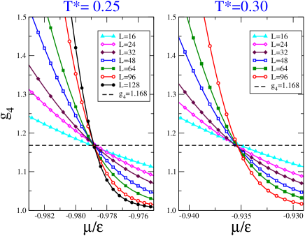
Figure 1: (Color on line) Fourth order Binder cumulant as a function of $\mu$ for different system sizes, at $T^{*}=0.25$ and $T^{*}=0.30$.

III.2 Computation of $\left(\partial\rho/\partial\mu\right)_{T}$

In Fig. 2 we plot the derivative of the density with respect to the chemical potential, $\rho^{\prime}_{\mu}$, as a function of $\mu$, for different system sizes, at the same temperatures $T^{*}=0.25$ and $T^{*}=0.30$.

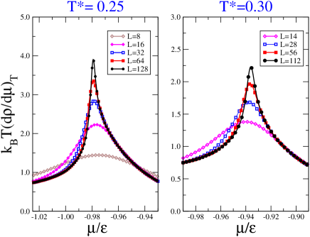
Figure 2: (Color on line) Derivative of the density, $\rho$, as a function of the chemical potential, $\mu$, for different system sizes, at $T^{*}=0.25$ and $T^{*}=0.30$. A singularity is clearly signalled at both temperatures.

At values of the chemical potential, $\mu$, close to its critical value, the derivative of the density, $\rho^{\prime}_{\mu}$, exhibits clear signs of singular behavior, with a peak that increases as the system size increases. The size dependence of the peaks is analyzed in Fig. 3.

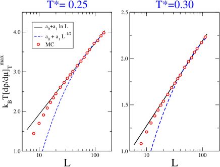
Figure 3: System size dependence of the maximum of $k_{B}T(\partial\rho/\partial\mu)_{T}$, at $T^{*}=0.25$ and $T^{*}=0.30$. Simulation results are represented by points. Lines are fits to the scaling laws discussed in the text.

The scaling of the peaks of $(\rho^{\prime}_{\mu})^{max}(L,T)$, with the system size $L$, is characteristic of the universality class of the transitionLandau_Binder . For SARR on the square lattice we anticipate either q=1 Potts (Q1UC) behavior ($\alpha/\nu=-1/2$) Wu as reported in Ref. Lopez or Q2UC behavior, as found for monodisperse rods on the same latticeMatoz2008b . In the latter case $\alpha/\nu=0$ and the peak is expected to diverge logarithmicallyWu . The two scaling laws are:

$$(\rho^{\prime}_{\mu})^{max}(L)=a_{0}+a_{1}L^{-1/2},\textrm{ for Q1UC},$$ (11)

$$(\rho^{\prime}_{\mu})^{max}(L)=a_{0}+a_{1}\ln L,\textrm{ for Q2UC}.$$ (12)

In Fig. 3, we plot fits of the two scaling laws to the simulation data. In both cases we discarded the data for the smallest system sizes. We found that the simulation results are better described by the 2D Ising scaling law, at all temperatures. In fact, equation (12) fits the data over a broader range of system sizes ($L\geq 24$ at $T^{*}=0.25$ and $L\geq 32$ at $T^{*}=0.30$) than does Eq. 11 ($L\geq 56$ at both temperatures).

III.3 Critical Line

We start by defining the pseudo-critical chemical potentials at fixed temperature. We consider the Binder cumulants, as functions of the chemical potential, and define the pseudo-critical chemical potentials, $\mu_{c}^{(L)}\equiv\mu_{c}(L)$ (at given $T$), such that:

$$g_{4}(L,\mu_{c}^{(L)},T)=g_{4}^{c}.$$ (13)

We have also used different definitions based on the position of the maxima of the density fluctuations and of $(\partial\ln<\delta>/\partial\mu)_{T}$, to check the consistency of the results. In Fig. 4 we plot the pseudo-critical chemical potentials as functions of $1/L$, at $T^{*}=0.25$ and $T^{*}=0.30$. At both temperatures, and $L\geq 32$, the chemical potential, $\mu_{c}(L)$, computed using Eq. (13) is almost independent of system size (horizontal lines in the left and right panels of Fig. 4).

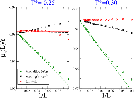
Figure 4: (Color on line) System size dependence of the pseudo-critical chemical potentials. See the text and the legend for details. Lines are least-squares fits to the MC results.

Estimates of the critical chemical potential, $\mu_{c}$, obtained by extrapolating the MC results, are collected in Table 1. Considering the behavior of $\mu_{c}(L)$ obtained using Eq. (13), we used the results of simulations at this chemical potential, to compute the critical density $\rho_{c}$ and the critical exponents. Assuming 2D Ising behavior, the critical density is given byLandau_Binder :

$$\rho_{c}(L,\mu_{c}^{(L)},T)=\rho_{c}(T)+aL^{-1}.$$ (14)

The results for the critical line $T_{c}(\rho)$ are plotted in Fig. 5. As expected, the temperature at the ordering transition decreases as the density decreases. The critical points calculated in earlier work (diamonds[Tavares2009a, ] and square[Lopez, ]) fall on the critical line, within the statistical error (open circles). The line of critical points of the SARR model continues beyond the lowest density reported in Fig. 5. However, the rapid increase of the average length of the rods at these (low) densities and temperatures prevents an efficient simulation of these systems with the currently available techniques.

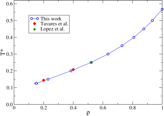
Figure 5: (Color on line) Critical line of the SARR model. The diamonds and square are from Refs. [Tavares2009a, ], and [Lopez, ], respectively.

III.4 Critical Exponents

The critical exponents $\beta/\nu$, and $\gamma/\nu$ Lopez ; Landau_Binder were estimated by fitting the MC results to the scaling laws,

$$\log\delta(L,\mu_{c}^{(L)},T)=a_{\beta}-\frac{\beta}{\nu}\log L,$$ (15)

and

$$\log\chi(L,\mu_{c}^{(L)},T)=a_{\xi}+\frac{\gamma}{\nu}\log L,$$ (16)

where the susceptibility $\chi$ is defined as:

$$\chi=L^{2}\left[<\delta^{2}>-<\delta>^{2}\right]/k_{B}T.$$ (17)

$T^{*}$	$\mu_{c}/\epsilon$	$\rho_{c}$	$<U/N\epsilon>_{c}$	$\beta/\nu$	$\gamma/\nu$
0.125	-1.0030(5)	0.15(1)	-0.944(1)	0.08(2)	1.86(3)
0.15	-1.0038(1)	0.230(3)	-0.919(1)	0.10(2)	1.79(4)
0.20	-0.9991(1)	0.384(1)	-0.874(1)	0.108(4)	1.761(9)
0.25	-0.9789(2)	0.520(1)	-0.843(1)	0.110(2)	1.757(4)
0.30	-0.9354(2)	0.634(1)	-0.826(1)	0.111(2)	1.754(3)
0.35	-0.8597(6)	0.729(1)	-0.818(1)	0.114(2)	1.750(2)
0.40	-0.7383(3)	0.8086(4)	-0.8188(3)	0.116(2)	1.751(3)
0.45	-0.5452(5)	0.8760(2)	-0.8249(3)	0.120(3)	1.749(3)
0.50	-0.214(2)	0.9338(4)	-0.8345(5)	0.123(2)	1.751(4)
0.5673	$\infty$	1.000	-0.85355	0.125	1.750

Table 1: Results for the critical parameters and effective critical exponents.

The critical parameters and effective exponents are collected in Table 1 at 10 different temperatures. Note that the exponents computed for $\beta/\nu$ lie between those corresponding to the Q1UC ($\beta/\nu=5/48\simeq 0.104$)Lopez ; Wu at low temperatures and those corresponding to the Q2UC ($\beta/\nu=1/8$)Wu at high temperatures. The results for $\gamma/\nu$ are closer to those of Q2UC ($\gamma/\nu=7/4$) over a wider range of temperature but at the lowest temperatures they also approach those of Q1UC ($\gamma/\nu=43/24\simeq 1.792$).

We note that Eq. (15) does not provide a good fit of the simulation results for a wide range of system sizes, and thus the results for $\beta/\nu$ should be regarded as effective exponents. Consideration of higher-order finite size corrections, of the form, $\delta_{c}(L)=L^{-\beta/\nu}\left[a_{0}+bL^{-\omega}\right]$, is not a feasible, as fits of the simulation results with four adjustable parameters cannot discriminate between these two, similar, scaling laws.

To proceed, we have investigated the finite-size scaling of the Binder cumulant, at $T^{*}=0.15$ and $T^{*}=0.40$. In Fig. 6 we plot $g_{4}(\mu)$ versus $L^{1/\nu}(\mu-\mu_{c})$, using for the critical exponent, $\nu$, the values corresponding to the q=1 ($\nu=4/3$) and q=2 ($\nu=1)$ universality classes. At $T^{*}=0.40$, the data collapse with $\nu=1$ is excellent, confirming that scaling for the Q2UC is satisfied for all the system sizes ($L\geq 48$). However, at the lowest temperature, $T^{*}=0.15$, the data collapse fails for both universality classes and systems with $L<80$. Nevertheless, the collapse observed with the Q2UC exponents is marginally better than that observed with the Q1UC exponents, suggesting that the SARR criticality is still in the 2D Ising class.

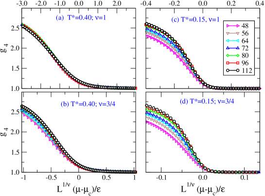
Figure 6: (Color on line) Fourth order Binder cumulant as a function of $\mu$ for different system sizes, at $T^{*}=0.15$ and $T^{*}=0.40$.

Finally, we analyzed the scaling behavior of the derivative of the logarithm of the order parameter with respect to the chemical potential, at constant temperature. The maxima of this quantity are expected to scale with the system size as Ferrenberg ; Landau_Binder ; Lopez $Q^{\prime}_{\mu}=\left(\partial\ln\delta/\partial\mu\right)_{T,L}^{\textrm{m}ax}\sim L^{1/\nu}$. On the basis of this scaling law, we have computed effective values of $1/\nu$ by Chi-square fittingNumerical_Recipes the simulation results to $Q^{\prime}_{\mu}(L)=aL^{1/\nu}$. The results for $1/\nu$ are collected in table 2, for several temperatures, and confirm that the SARR model is in the 2D Ising class. It is also clear that as the temperature decreases the effect of the finite system size becomes more important, i.e. one requires larger systems to stay on the asymptotic scaling region.

$T^{*}$	$n$	$L_{min}$	$L_{max}$	$\chi^{2}/{\textrm{d}.o.f}$	$1/\nu$
0.15	5	80	144	0.84	1.22(15)
0.20	5	80	144	1.71	1.13(10)
0.25	5	80	144	1.13	1.04(9)
0.30	8	48	112	0.08	1.05(4)
0.35	8	40	112	0.65	1.02(2)
0.40	10	32	112	1.33	1.00(2)

Table 2: Estimates of effective values of $1/\nu$ for different temperatures; $n$ is the number of points (system sizes) used in the fitting; $L_{min}$, and $L_{max}$ are the minimum and maximum system sizes considered, with $L_{min}$ chosen to provide statistically acceptable values for the $\chi^{2}$ merit function Numerical_Recipes . d.o.f. is the number of degrees of freedom in each fitting.

IV Analysis of the criticality of the SARR model

IV.1 The full lattice limit: 2D Ising

The results of the previous section suggest clearly that the criticality of the SARR model is in the 2D Ising class. In this section we investigate the full lattice limit of the SARR model, or full lattice limit (FLL) for short, where we can prove that this is indeed the case. One also expects the criticality to remain unchanged, as long as no other transitions occur on the critical lineSilva .

We performed a number of simulations using a multi-temperature algorithm proposed by Zhang and MaZhang and found that the critical temperature is the same as that of the lattice gas. This is more than a coincidence as shown below.

We have mapped the monomer orientations ${\hat{x}}$, ${\hat{y}}$ to the Ising spins $\pm 1$ and computed the total energy of the models by adding the contributions, $u_{p}$, of square elementary plaquettes,

$$U=\frac{1}{2}\sum_{p}^{N_{plaq}}u_{p},$$ (18)

where each plaquette consists of a square with four sites enclosing an elementary cell of the lattice, where we have taken into account that each pair interaction is counted in two different plaquettes. In Table 3 we collect the energies for representative plaquette configurations of both models.

	Plaquette	$\begin{array}[]{cc}+&+\\ +&+\end{array}$	$\begin{array}[]{cc}+&+\\ +&-\end{array}$	$\begin{array}[]{cc}+&+\\ -&-\end{array}$	$\begin{array}[]{cc}+&-\\ -&+\end{array}$
Ising	$u_{p}/\epsilon_{I}$	-4	0	0	4
SARR	$u_{p}/\epsilon$	- 2	-1	- 1	0

Table 3: Plaquette interactions in the Ising and the FLL of the SARR models on the square lattice.

The mapping between the two models, is then for any plaquette configuration:

$$u_{p}^{Ising}/\epsilon_{I}=4u_{p}^{FLL}/\epsilon+4.$$ (19)

implying that the FLL limit of the SARR model, on the square lattice, is in the 2D Ising universality class.

IV.2 The zero density limit: Self-assembly

The SARR model has two independent thermodynamic parameters, the temperature and the density of monomers. At high temperatures $k_{B}T>>\epsilon$ there is little bonding and the behavior of the model is similar to that of the lattice gas. At low temperatures, however, bonding dominates and the model behaves in a strikingly different way. Rods self-assemble and, at a fixed density, the average rod length increases exponentially as the temperature decreases. The polydisperse rods undergo an ordering transition at a density that is temperature dependent. The transition was calculated in Ref. Tavares2009a using a generalized mean-field theory of self-assembly, where the polydisperse rods interact through Onsager-like excluded volume terms only.

The critical line is given byTavares2009a :

$$\frac{1}{T^{*}_{c}}=\ln\left[\frac{(2-\rho_{c})(2+\rho_{c})}{2\rho_{c}^{3}}\right],$$ (20)

and is plotted in Fig. 7. This line is singular in the zero-density limit, where the average rod length diverges, signalling the self-assembly or equilibrium polymerization transition at zero temperature. An estimate of the crossover line, from the polymerzation transition, is obtained from the asymptotic relation between $T^{*}_{c}$ and $\rho_{c}$, at the singular point:

$$T^{*}_{c}\sim-\frac{1}{\ln\rho_{c}}.$$ (21)

Using the results for the thermodynamic potentials derived in Ref. Tavares2009a one finds that the chemical potential at the critical point, $\mu_{c}$, is given in terms of the critical temperature and density, $T_{c}$ and $\rho_{c}$:

$$\mu_{c}/\epsilon=T^{*}_{c}\left[\ln(2\rho_{c}^{3})+\rho_{c}/2-2\ln(2-\rho_{c})\right].$$ (22)

Using the asymptotic form, Eq. (21), we find for the crossover line:

$$\mu_{c}/\epsilon\sim-1.$$ (23)

This line delimits the region where the self-assembly or equilibrium polymerization fluctuations are large. In Fig. 7 we plot the critical and crossover lines of the SARR model as functions of $\mu$ and $\rho$. Note that the crossover line approaches the critical line tangentially in the equilibrium polymerization limit, suggesting that the asymptotic scaling region of the finite density critical point decreases rapidly as the critical temperature and density decrease.

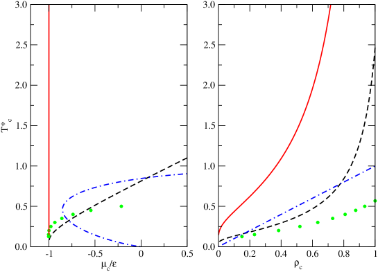
Figure 7: (Color on line) Critical lines from MC simulation (points), theory of self-assembly (dashed) and mean-field theory (dashed-dotted). Crossover line is the full line. Left panel: $\mu,T$ diagram. Right panel: $\rho,T$ diagram. See text for details.

Finally, the internal energy on the critical line is easily calculated and we findTavares2009a :

$$\frac{U}{N\epsilon}=-\frac{2\rho_{c}}{2+\rho_{c}}.$$ (24)

Note that the energy per particle increases monotonically with the (critical) density. This is plotted in Fig. 8 and will be discussed in the next section.

IV.3 Intermediate densities

A look at Table 1 reveals that the critical energy per particle, $u_{c}=<U/N>_{c}$, varies non-monotonically with the temperature. In the self-assembly limit, the internal energy $u^{*}=<U/N\epsilon>$ is a measure of the average rod length and is predicted to vary monotonically on the critical line, as stated above (see Ref.Tavares2009a for details). Clearly, a departure from this behavior indicates the importance of the attractions between rods, which are short in the high-temperature regime.

Let us assume that there is no bonding, i.e., the temperature is so high that the average rod length is of order 1. Then, on average, each monomer interacts with its aligned neighbors, the pairs being aligned with the corresponding lattice bonds. The mean-field free energy becomes:

$$\beta f=\sum_{\alpha=x,y}\rho_{\alpha}(\ln\rho_{\alpha}-1)+(1-\rho)(\ln(1-\rho)-1)-\beta\epsilon(\rho_{x}^{2}+\rho_{y}^{2}),$$ (25)

where $\rho_{x}$ and $\rho_{y}$ are the densities of particles aligned with the $\hat{x}$ and $\hat{y}$ directions, respectively, and we have accounted for the entropy of the empty lattice sites. Given that $\rho=\rho_{x}+\rho_{y}$ and defining $\Delta=\rho_{x}-\rho_{y}$, the free energy may be written in terms of these variables. The critical points are obtained by (i) calculating the field associated with $\Delta$, $\beta h=\frac{\partial\beta f}{\partial\Delta}$ and (ii) setting $h=0$ to obtain, implicitly, $\Delta(\rho,T)$. The critical line is given by:

$$T^{*}_{c}=\rho_{c}.$$ (26)

and the internal energy on the critical line becomes:

$$\frac{U}{N\epsilon}=-\frac{\rho_{c}}{2}.$$ (27)

The internal energy on the critical line is plotted in Fig. 8. The points are the computer simulation results while the two lines are obtained from the self-assembly and the high-temperature mean-field theories. The results from self-assembly, Eq. (24), are monotonically increasing, while those from the high temperature theory, Eq. (27), are monotonically decreasing.

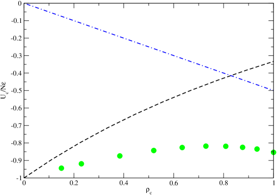
Figure 8: (Color on line) Internal energy per particle on the critical line. Points: MC simulation, dashed: theory of self-assembly, dashed-dotted: mean-field theory. See text for details.

The low density/temperature behavior is captured by the self-assembly theory Tavares2009a while the high density/temperature limit is described by the mean-field theory. Similar remarks apply to the critical line itself, as shown in Fig. 7.

This analysis suggests that although self-assembly fluctuations become increasingly important as the density decreases the nature of the singularity changes at $\rho=0$ only. Nevertheless, the scaling region decreases rapidly in the low-density/temperature region and the true asymptotic behavior may be difficult to observe in simulations of reasonably sized systems.

V Discussion

The results reported in the previous sections clearly suggest that the critical behavior of the SARR model is 2D Ising. This conclusion is supported by (i) the scaling behavior of the Binder cumulant for different system sizes, (ii) the system size dependence of the peaks of $\rho^{\prime}_{\mu}(\mu)$ and (iii) the values of the critical exponent $\nu$. This conclusion contrasts with that of López et al., and it is important to understand the reasons for this discrepancy. First we acknowledge that the values of $\beta/\nu$ are relatively similar for the two universality classes; the same may be said of $\gamma/\nu$. Thus the distinction between the two universality classes will have to be based on the value of the $g_{4}(L)$ crossing and on the value of $\nu$. In the analysis of López et al, the use of the density as the control parameter leads to a value of the $g_{4}$ crossing that differs substantially from that of the 2D Ising universality class. We have shown that using $\mu$ as the control parameter leads to a more robust scaling of $g_{4}$ and to a much better overall Ising scaling.

Concluding that the SARR model is indeed in the Ising universality class, the question is then, how was the value of $\nu\approx 4/3$ observed when using $\rho$ as the control parameter? Consider a property $Q$ whose derivative with respect to the control parameter has a maximum in the critical region. Such derivative scales in the finite size region asLopez ; Landau_Binder :

$$Q^{\prime}_{s}\equiv\left(\frac{\partial Q(L)}{\partial s}\right)^{max}=aL^{1/\nu}(1+bL^{-\omega}),$$ (28)

where $s$ represents either the density or the chemical potential. In the scaling region $Q^{\prime}_{\mu}$, and $Q^{\prime}_{\rho}$ are related by:

$$Q^{\prime}_{\rho}\approx Q^{\prime}_{\mu}\left(\frac{\partial\mu}{\partial\rho}\right)\sim\frac{L}{\ln L},$$ (29)

where we used $\nu=1$ (Q2UC) and the scaling relation given in Eq. (12). We suspect that the presence of $\ln L$ in the scaling of $Q^{\prime}_{\rho}$, raises the value of the effective critical exponent $\nu$. In particular, for the range $60\leq L\leq 120$ used by López et al. Lopez the ratio $L/\ln L$ is well described by: $L/\ln L\simeq aL^{1/\nu^{\prime}}$, with $\nu^{\prime}\simeq 1.291$, close to the value $\nu=4/3$ of the Q1UC. This is illustrated in Fig. 9 where it is clear that the finite-size scaling of $g_{4}(\rho,L)$ is well described using both $x=L^{-3/4}(\rho-\rho_{c})$ and $x=(\rho-\rho_{c})L/\ln L$ as the scaling density.

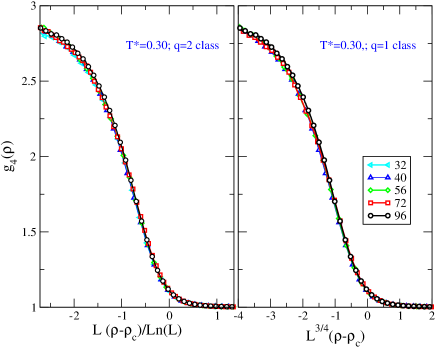
Figure 9: (Color on line) Fourth order Binder cumulants for different system sizes as a function of the scaling densities in the $q=1$ and $q=2$ universality classes, at $T^{*}=0.30$.

To conclude, we have shown that the criticality of the SARR model is 2D Ising. Nevertheless, as the temperature decreases deviations from the Ising scaling laws increase, and larger system sizes are needed to obtain accurate estimates of the critical exponents. This can be understood in terms of the self-assembly fluctuations that occur closer to the critical line as the density and temperature decrease. In addition, the use of PBC may enhance this finite-size effect, through the percolation of ’periodic’ rods.

Finally, we note that Milchev and Landau Milchev analysed the critical behavior of a flexible self-assembling rod model in 2D. They report a continuous transition in the $T,\mu$ space ending at a tricritical point, at finite density, and critical exponents on the continuous portion of the two-phase boundary in the 2D Ising class. Their model is richer than ours but the nature of the continuous portion of the phase boundary is likely to be the same. The connection between these two models as well as extensions to 3D will be left for future work.

- (1) D. Ioffe, Y. Velenik and M. Zahradník, J. Stat. Phys. 122, 761 (2006).
- (2) L. Onsager, Ann. N.Y. Acad. Sci. 51, 627 (1949).
- (3) J. P. Straley, Phys. Rev. A 4, 675 (1971).
- (4) D. Frenkel and R. Eppenga, Phys. Rev. A 31, 1776 (1985).
- (5) R. L. C. Vink, Phys. Rev. Lett. 98, 217801 (2007).
- (6) J. J. Potoff and J. I. Siepmann, Phys. Rev. Lett. 85, 3460 (2000).
- (7) D. A. Matoz-Fernandez, D. H. Linares and A. J. Ramirez-Pastor, J. Chem. Phys. 128, 214902 (2008).
- (8) D. A. Matoz-Fernandez, D. H. Linares and A. J. Ramirez-Pastor, Europhys. Lett. 82, 50007 (2008).
- (9) A. Ghosh and D. Dhar, Europhys. Lett. 78, 20003 (2007).
- (10) R. Zwanzig, J. Chem. Phys. 39, 1714 (1963).
- (11) N. Clarke, J. A. Cuesta, R. Sear, P. Sollich and A. Speranza, J. Chem. Phys. 113, 5817 (2000).
- (12) J. M. Tavares, B. Holder and M. M. Telo da Gama, Phys. Rev E 79, 021505 (2009).
- (13) H. Takasaki, T. Nishino and Y. Hieida, Journal of the Physical Society of Japan 70, 1429 (2001).
- (14) L. G. López, F. H. Linares and A. J. Ramirez-Pastor, Phys. Rev E 80, 040105(R)(2009).
- (15) J. M. Tavares, P. I. C. Teixeira and M. M. Telo da Gama, Phys. Rev. E 80, 021506 (2009).
- (16) J. M. Tavares, P. I. C. Teixeira and M. M. Telo da Gama, Phys. Rev. E 81, 010501(R) (2010).
- (17) J. S. Hoye, E. Lomba and N. G. Almarza, Mol. Phys. 107, 321 (2009).
- (18) N. G. Almarza, J. A. Capitán, J. A. Cuesta and E. Lomba, J. Chem. Phys. 131, 124506 (2009).
- (19) E. Lomba, N. G. Almarza, C. Martín and C. McBride , J. Chem. Phys. 126, 244510 (2007).
- (20) F. Wang and D. P. Landau, Phys. Rev. Lett. 86, 2050 (2001).
- (21) D. P. Landau and K. Binder, ”A Guide to Monte Carlo Simulation in Statistical Physics, 2nd edition”, (Cambridge University Press 2005).
- (22) J. Salas and A.D. Sokal, J. Stat. Phys. 98, 551 (2000).
- (23) F.Y. Wu, Rev. Mod. Phys., 54, 235 (1982).
- (24) A.M. Ferrenberg and D.P. Landau, Phys. Rev. B 44, 5081 (1991).
- (25) W.H. Press, S.A. Teukolsky, W.T. Vetterling, and B.P. Flannery, ”Numerical Recipes. The Art of Scientific Computing, 3rd edition”, (Cambridge University Press).
- (26) C.J. Silva, A.A. Caparica and J.A. Plascak, Phys. Rev. E 73, 036702 (2006).
- (27) C. Zhang and J. Ma, Phys. Rev. E, 76, 036708 (2007).
- (28) A. Milchev and D. P. Landau, Phys. Rev. E 52, 6431 (1995).