Inconsistency of bootstrap: The Grenander estimator

Abstract

In this paper, we investigate the (in)-consistency of different bootstrap methods for constructing confidence intervals in the class of estimators that converge at rate $n^{1/3}$. The Grenander estimator, the nonparametric maximum likelihood estimator of an unknown nonincreasing density function $f$ on $[0,\infty)$, is a prototypical example. We focus on this example and explore different approaches to constructing bootstrap confidence intervals for $f(t_{0})$, where $t_{0}\in(0,\infty)$ is an interior point. We find that the bootstrap estimate, when generating bootstrap samples from the empirical distribution function $\mathbb{F}_{n}$ or its least concave majorant $\tilde{F}_{n}$, does not have any weak limit in probability. We provide a set of sufficient conditions for the consistency of any bootstrap method in this example and show that bootstrapping from a smoothed version of $\tilde{F}_{n}$ leads to strongly consistent estimators. The $m$ out of $n$ bootstrap method is also shown to be consistent while generating samples from $\mathbb{F}_{n}$ and $\tilde{F}_{n}$.

,
and

t1Supported by NSF Grant DMS-09-06597. t2Supported by NSF Grant DMS-07-05288. t3Supported by NSF Grant AST-05-07453.

1 Introduction

If $X_{1},X_{2},\ldots,X_{n}\stackrel{{\scriptstyle\mathrm{ind}}}{{\sim}}f$ are a sample from a nonincreasing density $f$ on $[0,\infty)$, then the Grenander estimator, the nonparametric maximum likelihood estimator (NPMLE) $\tilde{f}_{n}$ of $f$ [obtained by maximizing the likelihood $\prod_{i=1}^{n}f(X_{i})$ over all nonincreasing densities], may be described as follows: let $\mathbb{F}_{n}$ denote the empirical distribution function (EDF) of the data, and $\tilde{F}_{n}$ its least concave majorant. Then the NPMLE $\tilde{f}_{n}$ is the left-hand derivative of $\tilde{F}_{n}$. This result is due to Grenander (1956) and is described in detail by Robertson, Wright and Dykstra (1988), pages 326–328. Prakasa Rao (1969) obtained the asymptotic distribution of $\tilde{f}_{n}$, properly normalized: let $\mathbb{W}$ be a two-sided standard Brownian motion on $\mathbb{R}$ with $\mathbb{W}(0)=0$ and

$${\mathbb{C}}=\mathop{\arg\max}_{s\in{\mathbb{R}}}[{\mathbb{W}}(s)-s^{2}].$$

If $0<t_{0}<\infty$ and $f^{\prime}(t_{0})\neq 0$, then

$$n^{1/3}\{\tilde{f}_{n}(t_{0})-f(t_{0})\}\Rightarrow 2\bigl{|}\tfrac{1}{2}f(t_{0})f^{\prime}(t_{0})\bigr{|}^{1/3}{\mathbb{C}},$$ (1)

where $\Rightarrow$ denotes convergence in distribution. There are other estimators that exhibit similar asymptotic properties; for example, Chernoff’s (1964) estimator of the mode, the monotone regression estimator [Brunk (1970)], Rousseeuw’s (1984) least median of squares estimator, and the estimator of the shorth [Andrews et al. (1972) and Shorack and Wellner (1986)]. The seminal paper by Kim and Pollard (1990) unifies $n^{1/3}$-rate of convergence problems in the more general $M$-estimation framework. Tables and a survey of statistical problems in which the distribution of ${\mathbb{C}}$ arises are provided by Groeneboom and Wellner (2001).

The presence of nuisance parameters in the limiting distribution (1) complicates the construction of confidence intervals. Bootstrap intervals avoid the problem of estimating nuisance parameters and are generally reliable in problems with $\sqrt{n}$ convergence rates. See Bickel and Freedman (1981), Singh (1981), Shao and Tu (1995) and its references. Our aim in this paper is to study the consistency of bootstrap methods for the Grenander estimator with the hope that the monotone density estimation problem will shed light on the behavior of bootstrap methods in similar cube-root convergence problems.

There has been considerable recent interest in this question. Kosorok (2008) show that bootstrapping from the EDF ${\mathbb{F}}_{n}$ does not lead to a consistent estimator of the distribution of $n^{1/3}\{\tilde{f}_{n}(t_{0})-f(t_{0})\}$. Lee and Pun (2006) explore $m$ out of $n$ bootstrapping from the empirical distribution function in similar nonstandard problems and prove the consistency of the method. Léger and MacGibbon (2006) describe conditions for a resampling procedure to be consistent under cube root asymptotics and assert that these conditions are generally not met while bootstrapping from the EDF. They also propose a smoothed version of the bootstrap and show its consistency for Chernoff’s estimator of the mode. Abrevaya and Huang (2005) show that bootstrapping from the EDF leads to inconsistent estimators in the setup of Kim and Pollard (1990) and propose corrections. Politis, Romano and Wolf (1999) show that subsampling based confidence intervals are consistent in this scenario.

Our work goes beyond that cited above as follows: we show that bootstrapping from the NPMLE $\tilde{F}_{n}$ also leads to inconsistent estimators, a result that we found more surprising, since $\tilde{F}_{n}$ has a density. Moreover, we find that the bootstrap estimator, constructed from either the EDF or NPMLE, has no limit in probability. The finding is less than a mathematical proof, because one step in the argument relies on simulation; but the simulations make our point clearly. As described in Section 5, our findings are inconsistent with some claims of Abrevaya and Huang (2005). Also, our way of tackling the main issues differs from that of the existing literature: we consider conditional distributions in more detail than Kosorok (2008), who deduced inconsistency from properties of unconditional distributions; we directly appeal to the characterization of the estimators and use a continuous mapping principle to deduce the limiting distributions instead of using the “switching” argument [see Groeneboom (1985)] employed by Kosorok (2008) and Abrevaya and Huang (2005); and at a more technical level, we use the Hungarian Representation theorem whereas most of the other authors use empirical process techniques similar to those described by van der Vaart and Wellner (2000).

Section 2 contains a uniform version of (1) that is used later on to study the consistency of different bootstrap methods and may be of independent interest. The main results on inconsistency are presented in Section 3. Sufficient conditions for the consistency of a bootstrap method are presented in Section 4 and applied to show that bootstrapping from smoothed versions of $\tilde{F}_{n}$ does produce consistent estimators. The $m$ out of $n$ bootstrapping procedure is investigated, when generating bootstrap samples from $\mathbb{F}_{n}$ and $\tilde{F}_{n}$. It is shown that both the methods lead to consistent estimators under mild conditions on $m$. In Section 5, we discuss our findings, especially the nonconvergence and its implications. The Appendix, provides the details of some arguments used in proving the main results.

2 Uniform convergence

For the rest of the paper, $F$ denotes a distribution function with $F(0)=0$ and a density $f$ that is nonincreasing on $[0,\infty)$ and continuously differentiable near $t_{0}\in(0,\infty)$ with nonzero derivative $f^{\prime}(t_{0})<0$. If $g\dvtx I\to{\mathbb{R}}$ is a bounded function, write $\|g\|:={\sup_{x\in I}}|g(x)|$. Next, let $F_{n}$ be distribution functions with $F_{n}(0)=0$, that converge weakly to $F$ and, therefore,

$${\lim_{n\to\infty}}\|F_{n}-F\|=0.$$ (2)

Let $X_{n,1},X_{n,2},\ldots,X_{n,m_{n}}\stackrel{{\scriptstyle\mathrm{ind}}}{{\sim}}F_{n}$, where $m_{n}\leq n$ is a nondecreasing sequence of integers for which $m_{n}\to\infty$; let ${\mathbb{F}}_{n,m_{n}}$ denote the EDF of $X_{n,1},X_{n,2},\ldots,\break X_{n,m_{n}}$; and let

$$\Delta_{n}:=m_{n}^{1/3}\{\tilde{f}_{n,m_{n}}(t_{0})-f_{n}(t_{0})\},$$

where $\tilde{f}_{n,m_{n}}(t_{0})$ is the Grenander estimator computed from $X_{n,1},X_{n,2},\ldots,\break X_{n,m_{n}}$ and $f_{n}(t_{0})$ is the density of $F_{n}$ at $t_{0}$ or a surrogate. Next, let $I_{m}=[-t_{0}m^{1/3},\infty)$ and

$$\quad\mathbb{Z}_{n}(h):=m_{n}^{2/3}\{\mathbb{F}_{n,m_{n}}(t_{0}+m_{n}^{-{1/3}}h)-\mathbb{F}_{n,m_{n}}(t_{0})-f_{n}(t_{0})m_{n}^{-{1/3}}h\}$$ (3)

for $h\in I_{m_{n}}$ and observe that $\Delta_{n}$ is the left-hand derivative at $0$ of the least concave majorant of ${\mathbb{Z}}_{n}$. It is fairly easy to obtain the asymptotic distribution of $\mathbb{Z}_{n}$. The asymptotic distribution of $\Delta_{n}$ may then be obtained from the Continuous Mapping theorem. Stochastic processes are regarded as random elements in $D(\mathbb{R})$, the space of right continuous functions on $\mathbb{R}$ with left limits, equipped with the projection $\sigma$-field and the topology of uniform convergence on compacta. See Pollard (1984), Chapters IV and V for background.

2.1 Convergence of ${\mathbb{Z}}_{n}$

It is convenient to decompose $\mathbb{Z}_{n}$ into the sum of $\mathbb{Z}_{n,1}$ and $\mathbb{Z}_{n,2}$ where

$$\mathbb{Z}_{n,1}(h) := m_{n}^{2/3}\{(\mathbb{F}_{n,m_{n}}-F_{n})(t_{0}+m_{n}^{-{1/3}}h)-(\mathbb{F}_{n,m_{n}}-F_{n})(t_{0})\},$$

$$\mathbb{Z}_{n,2}(h) := m_{n}^{2/3}\{F_{n}(t_{0}+m_{n}^{-{1/3}}h)-F_{n}(t_{0})-f_{n}(t_{0})m_{n}^{-{1/3}}h\}.$$

Observe that ${\mathbb{Z}}_{n,2}$ depends only on $F_{n}$ and $f_{n}$; only ${\mathbb{Z}}_{n,1}$ depends on $X_{n,1},\ldots,\break X_{n,m_{n}}$. Let $\mathbb{W}_{1}$ be a standard two-sided Brownian motion on $\mathbb{R}$ with $\mathbb{W}_{1}(0)=0$, and $\mathbb{Z}_{1}(h)=\mathbb{W}_{1}[f(t_{0})h]$.

Proposition 2.1

If

$$\lim_{n\to\infty}m_{n}^{1/3}|F_{n}(t_{0}+m_{n}^{-{1/3}}h)-F_{n}(t_{0})-f(t_{0})m_{n}^{-{1/3}}h|=0$$ (4)

uniformly on compacts (in $h$), then ${\mathbb{Z}}_{n,1}\Rightarrow{\mathbb{Z}}_{1}$; and if there is a continuous function ${\mathbb{Z}}_{2}$ for which

$$\lim_{n\to\infty}{\mathbb{Z}}_{n,2}(h)={\mathbb{Z}}_{2}(h)$$ (5)

uniformly on compact intervals, then ${\mathbb{Z}}_{n}\Rightarrow{\mathbb{Z}}:={\mathbb{Z}}_{1}+{\mathbb{Z}}_{2}$.

The Hungarian Embedding theorem of Kómlos, Major andTusnády (1975) is used. We may suppose that $X_{n,i}=F_{n}^{\#}(U_{i})$, where $F_{n}^{\#}(u)=\inf\{x\dvtx F_{n}(x)\geq u\}$ and $U_{1},U_{2},\ldots$ are i.i.d. Uniform$(0,1)$ random variables. Let $\mathbb{U}_{n}$ denote the EDF of $U_{1},\ldots,U_{n}$, $\mathbb{E}_{n}(t)=\sqrt{n}[\mathbb{U}_{n}(t)-t]$, and $\mathbb{V}_{n}=\sqrt{m_{n}}(\mathbb{F}_{n,m_{n}}-F_{n})$. Then $\mathbb{V}_{n}=\mathbb{E}_{m_{n}}\circ F_{n}$. By Hungarian Embedding, we may also suppose that the probability space supports a sequence of Brownian Bridges $\{\mathbb{B}_{n}^{0}\}_{n\geq 1}$ for which

$${\sup_{0\leq t\leq 1}}|\mathbb{E}_{n}(t)-\mathbb{B}_{n}^{0}(t)|=O\biggl{[}{\log(n)\over\sqrt{n}}\biggr{]}\qquad\mbox{a.s.},$$ (6)

and a standard normal random variable $\eta$ that is independent of $\{\mathbb{B}_{n}^{0}\}_{n\geq 1}$. Define a version $\mathbb{B}_{n}$ of Brownian motion by $\mathbb{B}_{n}(t)=\mathbb{B}_{n}^{0}(t)+\eta t$, for $t\in[0,1]$. Then

$$\mathbb{Z}_{n,1}(h) = m_{n}^{1/6}\{\mathbb{E}_{m_{n}}[F_{n}(t_{0}+m_{n}^{-{1/3}}h)]-\mathbb{E}_{m_{n}}[F_{n}(t_{0})]\}$$

$$= m_{n}^{1/6}\{\mathbb{B}_{m_{n}}[F_{n}(t_{0}+m_{n}^{-{1/3}}h)]-\mathbb{B}_{m_{n}}[F_{n}(t_{0})]\}+\mathbb{R}_{n}(h),$$

where

$$|\mathbb{R}_{n}(h)| \leq 2m_{n}^{1/6}{\sup_{0\leq t\leq 1}}|\mathbb{E}_{m_{n}}(t)-\mathbb{B}_{m_{n}}^{0}(t)|$$

$${}+m_{n}^{1/6}|\eta||F_{n}(t_{0}+m_{n}^{-{1/3}}h)-F_{n}(t_{0})|\rightarrow 0$$

uniformly on compacta w.p. 1 using (4) and (6). Let

$$\mathbb{X}_{n}(h):=m_{n}^{1/6}\{\mathbb{B}_{m_{n}}[F_{n}(t_{0}+m_{n}^{-{1/3}}h)]-\mathbb{B}_{m_{n}}[F_{n}(t_{0})]\}$$

and observe that $\mathbb{X}_{n}$ is a mean zero Gaussian process defined on $I_{m_{n}}$ with independent increments and covariance kernel

$$K_{n}(h_{1},h_{2})=m_{n}^{1/3}|F_{n}[t_{0}+\operatorname{sign}\{h_{1}\}m_{n}^{-{1/3}}(|h_{1}|\wedge|h_{2}|)]-F_{n}(t_{0})|\mathbf{1}\{h_{1}h_{2}>0\}.$$

It now follows from Theorem V.19 in Pollard (1984) and (4) that $\mathbb{X}_{n}(h)$ converges in distribution to $\mathbb{W}_{1}[f(t_{0})h]$ in $D([-c,c])$ for every $c>0$, establishing the first assertion of the proposition. The second then follows from Slutsky’s theorem.

2.2 Convergence of $\Delta_{n}$

Unfortunately, $\Delta_{n}$ is not quite a continuous functional of ${\mathbb{Z}}_{n}$. If $f\dvtx I\to{\mathbb{R}}$, write $f|J$ to denote the restriction of $f$ to $J\subseteq I$; and if $I$ and $J$ are intervals and $f$ is bounded, write $L_{J}f$ for the least concave majorant of the restriction. Thus, $\tilde{F}_{n}=L_{[0,\infty)}{\mathbb{F}}_{n}$ in the Introduction.

Lemma 2.2

Let $I$ be a closed interval; let $f\dvtx I\to{\mathbb{R}}$ be a bounded upper semi-continuous function on $I$; and let $a_{1},a_{2},b_{1},b_{2}\in I$ with $b_{1}<a_{1}<a_{2}<b_{2}$. If $2f[{1\over 2}(a_{i}+b_{i})]>L_{I}f(a_{i})+L_{I}f(b_{i}),i=1,2$, then $L_{I}f(x)=L_{[b_{1},b_{2}]}f(x)$ for $a_{1}\leq x\leq a_{2}$.

This follows from the proof of Lemmas 5.1 and 5.2 of Wang and Woodroofe (2007). In that lemma continuity was assumed, but only upper semi-continuity was used in the (short) proof.

Recall Marshall’s lemma: if $I$ is an interval, $f:I\to{\mathbb{R}}$ is bounded, and $g\dvtx I\to{\mathbb{R}}$ is concave, then $\|L_{I}f-g\|\leq\|f-g\|$. See, for example, Robertson, Wright and Dykstra [(1988), page 329] for a proof. Write $\tilde{F}_{n,m_{n}}=L_{[0,\infty)}{\mathbb{F}}_{n,m_{n}}$.

Lemma 2.3

If $\delta>0$ is so small that $F$ is strictly concave on $[t_{0}-2\delta,t_{0}+2\delta]$ and (2) holds then ${\tilde{F}}_{n,m_{n}}=L_{[t_{0}-2\delta,t_{0}+2\delta]}{\mathbb{F}}_{n,m_{n}}$ on $[t_{0}-\delta,t_{0}+\delta]$ for all large $n$ w.p. 1.

Since $F$ is strictly concave on $[t_{0}-2\delta,t_{0}+2\delta],2F(t_{0}\pm{3\over 2}\delta)>F(t_{0}\pm\delta)+F(t_{0}\pm 2\delta)$. Then

$$\|\tilde{F}_{n,m_{n}}-F\| \leq \|{\mathbb{F}}_{n,m_{n}}-F\|$$

$$\leq \|{\mathbb{F}}_{n,m_{n}}-F_{n}\|+\|F_{n}-F\|$$

$$\leq \frac{1}{\sqrt{m_{n}}}\|\mathbb{E}_{m_{n}}\|+\|F_{n}-F\|\to 0\qquad\mbox{w.p. }1$$

by Marshall’s lemma, (2) and the Glivenko–Cantelli theorem. Thus,$2{\mathbb{F}}_{n,m_{n}}(t_{0}\pm{3\over 2}\delta)>\tilde{F}_{n,m_{n}}(t_{0}\pm\delta)+\tilde{F}_{n,m_{n}}(t_{0}\pm 2\delta)$, for all large $n$ w.p. 1, and Lemma 2.3 follows from Lemma 2.2.

Proposition 2.4

(i) Suppose that (2) and (4) hold and given $\gamma>0$, there are $0<\delta<1$ and $C>0$ for which

$$\bigl{|}F_{n}(t_{0}+h)-F_{n}(t_{0})-f_{n}(t_{0})h-\tfrac{1}{2}f^{\prime}(t_{0})h^{2}\bigr{|}\leq\gamma h^{2}+Cm_{n}^{-{2/3}}$$ (8)

and

$$|F_{n}(t_{0}+h)-F_{n}(t_{0})|\leq C(|h|+m_{n}^{-{1/3}})$$ (9)

for $|h|\leq\delta$ and for all large $n$. If $J$ is a compact interval and $\varepsilon>0$, then there is a compact $K\supseteq J$, depending only on $\varepsilon,J,C,\gamma$, and $\delta$, for which

$$P[L_{I_{m_{n}}}{\mathbb{Z}}_{n}=L_{K}{\mathbb{Z}}_{n}\mbox{ on }J]\geq 1-\varepsilon$$ (10)

for all large $n$.

(ii) Let $\mathbb{Y}$ be an a.s. continuous stochastic process on $\mathbb{R}$ that is a.s. bounded above. If $\lim_{|h|\rightarrow\infty}\mathbb{Y}(h)/|h|=-\infty$ a.e., then the compact $K\supseteq J$ can be chosen so that

$$P[L_{\mathbb{R}}{\mathbb{Y}}=L_{K}{\mathbb{Y}}\mbox{ on }J]\geq 1-\varepsilon.$$ (11)

For a fixed sequence ($F_{n}\equiv F$) (10) would follow from the assertion in Example 6.5 of Kim and Pollard (1990), and it is possible to adapt their argument to a triangular array using (8) and (9) in place of Taylor series expansion. A different proof is presented in the Appendix.

We will use the following easily verified fact. In its statement, the metric space $\mathcal{X}$ is to be endowed with the projection $\sigma$-field. See Pollard (1984), page 70.

Lemma 2.5

Let $\{X_{n,c}\},\{Y_{n}\},\{W_{c}\}$ and $Y$ be sets of random elements taking values in a metric space $(\mathcal{X}$,$d)$, $n=0,1,\ldots,$ and $c\in\mathbb{R}$. If for any $\delta>0$,

$\lim_{c\rightarrow\infty}\limsup_{n\rightarrow\infty}P\{d(X_{n,c},Y_{n})>\delta\}=0$,

$\lim_{c\rightarrow\infty}P\{d(W_{c},Y)>\delta\}=0$,

$X_{n,c}\Rightarrow W_{c}$ as $n\rightarrow\infty$ for every $c\in\mathbb{R}$, then $Y_{n}\Rightarrow Y$ as $n\rightarrow\infty$.

Corollary 2.6

If (10) and (11) hold, and $\mathbb{Z}_{n}\Rightarrow\mathbb{Y}$, then $L_{I_{m_{n}}}{\mathbb{Z}}_{n}\Rightarrow L_{\mathbb{R}}{\mathbb{Y}}$ in $D({\mathbb{R}})$ and $\Delta_{n}\Rightarrow(L_{\mathbb{R}}{\mathbb{Y}})^{\prime}(0)$.

It suffices to show that $L_{I_{m_{n}}}{\mathbb{Z}}_{n}|J\Rightarrow L_{\mathbb{R}}{\mathbb{Y}}|J$ in $D(J)$, for every compact interval $J\subseteq\mathbb{R}$. Given $J$ and $\varepsilon>0$, there exists $K_{\varepsilon}$, a compact, $K_{\varepsilon}\supseteq J$, such that (10) and (11) hold. This verifies (i) and (ii) of Lemma 2.5 with $c=1/\varepsilon$, $X_{n,c}=L_{K_{\varepsilon}}{\mathbb{Z}}_{n}$, $Y_{n}=L_{I_{m_{n}}}{\mathbb{Z}}_{n}$, $W_{c}=L_{K_{\varepsilon}}{\mathbb{Y}}$, $Y=L_{\mathbb{R}}{\mathbb{Y}}$ and $d(x,y)=\sup_{t\in J}|x(t)-y(t)|$. Clearly, $L_{K_{\varepsilon}}{\mathbb{Z}}_{n}|J\Rightarrow L_{K_{\varepsilon}}{\mathbb{Y}}|J$ in $D(J)$, by the Continuous Mapping theorem, verifying condition (iii). Thus, $L_{I_{m_{n}}}{\mathbb{Z}}_{n}\Rightarrow L_{\mathbb{R}}{\mathbb{Y}}$ in $D(\mathbb{R})$. Another application of the Continuous Mapping theorem [via the lemma on page 330 of Robertson, Wright and Dykstra (1988)] in conjunction with (10), (11) and Lemma 2.5 then shows that $\Delta_{n}=(L_{I_{m_{n}}}{\mathbb{Z}}_{n})^{\prime}(0)\Rightarrow(L_{\mathbb{R}}{\mathbb{Y}})^{\prime}(0)$.

Corollary 2.7

If (2), (4), (5), (8) and (9) hold and

$$\lim_{|h|\rightarrow\infty}\mathbb{Z}(h)/|h|=-\infty,$$

then $L_{I_{m_{n}}}{\mathbb{Z}}_{n}\Rightarrow L_{\mathbb{R}}{\mathbb{Z}}$ in $D({\mathbb{R}})$ and $\Delta_{n}\Rightarrow(L_{\mathbb{R}}{\mathbb{Z}})^{\prime}(0)$; and if $\mathbb{Z}_{2}(h)=f^{\prime}(t_{0})h^{2}/2$, then $\Delta_{n}\Rightarrow 2|\frac{1}{2}f(t_{0})f^{\prime}(t_{0})|^{1/3}\mathbb{C}$, where $\mathbb{C}$ has Chernoff’s distribution.

The convergence follows directly from Proposition 2.4 andCorollary 2.6. Note that if $\mathbb{Z}_{2}(h)=f^{\prime}(t_{0})h^{2}/2$, then (10) and (11) holdand Corollary 2.6 can be applied. That $(L_{\mathbb{R}}{\mathbb{Z}})^{\prime}(0)$ is distributed as$2|\frac{1}{2}f(t_{0})f^{\prime}(t_{0})|^{1/3}\mathbb{C}$ when $\mathbb{Z}_{2}(h)=f^{\prime}(t_{0})h^{2}/2$ follows from elementary properties of Brownian motion via the “switching” argument of Groeneboom (1985).

2.3 Remarks on the conditions

If $F_{n}\equiv F$ and $f_{n}\equiv f$, then clearly (2), (4), (5), (8) and (9) all hold with ${\mathbb{Z}}_{2}(h)=f^{\prime}(t_{0})h^{2}/2$ for some $0<\delta<1$ and $C\geq f(t_{0}-\delta)$ by a Taylor expansion of $F$ and the continuity of $f$ and $f^{\prime}$ around $t_{0}$.

Corollary 2.8

If there is a $\delta>0$ for which $F_{n}$ has a continuously differentiable density $f_{n}$ on $[t_{0}-\delta,t_{0}+\delta]$, and

$$\quad\lim_{n\rightarrow\infty}\Bigl{[}\|F_{n}-F\|+\sup_{|t-t_{0}|<\delta}\bigl{(}|f_{n}(t)-f(t)|+|f_{n}^{\prime}(t)-f^{\prime}(t)|\bigr{)}\Bigr{]}=0,$$ (12)

then (2), (4), (5), (8) and (9) hold with ${\mathbb{Z}}_{2}(h)=f^{\prime}(t_{0})h^{2}/2$, and $\Delta_{n}\Rightarrow 2|\frac{1}{2}f(t_{0})f^{\prime}(t_{0})|^{1/3}\mathbb{C}$.

The result can be immediately derived from Taylor expansion of $F_{n}$ and the continuity of $f$ and $f^{\prime}$ around $t_{0}$. To illustrate the idea, we show that (8) holds. Let $\gamma>0$ be given. Clearly,

$$\biggl{|}F_{n}(t_{0}+h)-F_{n}(t_{0})-f_{n}(t_{0})h-\frac{1}{2}h^{2}f^{\prime}(t_{0})\biggr{|}$$

(13)

$$\qquad\leq{\frac{1}{2}h^{2}\sup_{|s|\leq|h|}}|f_{n}^{\prime}(t_{0}+s)-f^{\prime}(t_{0})|.$$

Let $\delta>0$ be so small that $|f^{\prime}(t)-f^{\prime}(t_{0})|\leq\gamma$ for $|t-t_{0}|<\delta$, and let $n_{0}$ be so large that ${\sup_{|t-t_{0}|\leq\delta}}|f_{n}^{\prime}(t)-f^{\prime}(t)|\leq\gamma$ for $n\geq n_{0}$. Then the last line in (2.3) is at most $\gamma h^{2}$ for $|h|\leq\delta$ and $n\geq n_{0}$.

Another useful remark, used below, is that if $\lim_{n\rightarrow\infty}m_{n}^{1/3}\|F_{m_{n}}-F\|=0$, then (2), (4) and (9) hold.

In the next three sections, we apply Proposition 2.1 and Corollary 2.6 to bootstrap samples drawn from the EDF, its LCM, and smoothed versions thereof. Thus, let $X_{1},X_{2},\ldots\stackrel{{\scriptstyle\mathrm{ind}}}{{\sim}}F$; let ${\mathbb{F}}_{n}$ be the EDF of $X_{1},\ldots,X_{n}$; and let $\tilde{F}_{n}$ be its LCM. If $F_{n}={\mathbb{F}}_{n}$, then (2), (4) and (9) hold almost surely by the above remark, since

$$\|{\mathbb{F}}_{n}-F\|=O\Biggl{[}\sqrt{\log\log(n)\over n}\Biggr{]}\qquad\mbox{a.s.}$$ (14)

by the Law of the Iterated Logarithm for the EDF, which may be deduced from Hungarian Embedding; and the same is true if $F_{n}=\tilde{F}_{n}$ since $\|\tilde{F}_{n}-F\|\leq\|{\mathbb{F}}_{n}-F\|$, by Marshall’s lemma.

If $m_{n}=n$ and $f_{n}=\tilde{f}_{n}$, then (5) is not satisfied almost surely or in probability by either ${\mathbb{F}}_{n}$ or $\tilde{F}_{n}$. For either choice, (8) is satisfied in probability if $f_{n}=f$.

Proposition 2.9

Suppose that $m_{n}=n$ and that $f_{n}=f$. If $F_{n}$ is either the EDF ${\mathbb{F}}_{n}$ or its LCM $\tilde{F}_{n}$, then for any $\gamma,\varepsilon>0$, there are $C>0$ and $0<\delta<1$ for which (8) holds with probability at least $1-\varepsilon$ for all large $n$.

The proof is included in the Appendix.

3 Inconsistency and nonconvergence of the bootstrap

We begin with a brief discussion of the bootstrap.

3.1 Generalities

Now, suppose that $X_{1},X_{2},\ldots\stackrel{{\scriptstyle\mathrm{ind}}}{{\sim}}F$ are defined on a probability space $(\Omega,\mathcal{A},P)$. Write ${\mathbf{X}}_{n}=(X_{1},\ldots,X_{n})$ and suppose that the distribution function, $H_{n}$ say, of the random variable $R_{n}(\mathbf{X}_{n},F)$ is of interest. The bootstrap methodology can be broken into three simple steps:

Construct an estimator $\hat{F}_{n}$ of $F$ from ${\mathbf{X}}_{n}$;

let $X_{1}^{*},\ldots,X_{m_{n}}^{*}\stackrel{{\scriptstyle\mathrm{ind}}}{{\sim}}\hat{F}_{n}$ be conditionally i.i.d. given ${\mathbf{X}}_{n}$;

then let ${\mathbf{X}}_{n}^{*}=(X_{1}^{*},\ldots,X_{m_{n}}^{*})$ and estimate $H_{n}$ by the conditional distribution function of $R_{n}^{*}=R({\mathbf{X}}_{n}^{*},\hat{F}_{n})$ given ${\mathbf{X}}_{n}$; that is

$$H_{n}^{*}(x)=P^{*}\{R^{*}_{n}\leq x\},$$

where $P^{*}\{\cdot\}$ is the conditional probability given the data $\mathbf{X}_{n}$, or equivalently, the entire sequence $\mathbf{X}=(X_{1},X_{2},\ldots)$. Choices of $\hat{F}_{n}$ considered below are the EDF ${\mathbb{F}}_{n}$, its least concave majorant $\tilde{F}_{n}$, and smoothed versions thereof.

Let $d$ denote the Levy metric or any other metric metrizing weak convergence of distribution functions. We say that $H_{n}^{*}$ is weakly, respectively, strongly, consistent if $d(H_{n},H_{n}^{*})\stackrel{{\scriptstyle P}}{{\rightarrow}}0$, respectively, $d(H_{n},H_{n}^{*})\to 0$ a.s. If $H_{n}$ has a weak limit $H$, then consistency requires $H_{n}^{*}$ to converge weakly to $H$, in probability; and if $H$ is continuous, consistency requires

$${\sup_{x\in\mathbb{R}}}|H_{n}^{*}(x)-H(x)|\stackrel{{\scriptstyle P}}{{\rightarrow}}0\qquad\mbox{as }n\rightarrow\infty.$$

There is also the apparent possibility that $H_{n}^{*}$ could converge to a random limit; that is, that there is a $G\dvtx\Omega\times\mathbb{R}\to[0,1]$ for which $G(\omega,\cdot)$ is a distribution function for each $\omega\in\Omega$, $G(\cdot,x)$ is measurable for each $x\in\mathbb{R}$, and $d(G,H_{n}^{*})\stackrel{{\scriptstyle P}}{{\rightarrow}}0$. This possibility is only apparent, however, if $\hat{F}_{n}$ depends only on the order statistics. For if $h$ is a bounded continuous function on $\mathbb{R}$, then any limit in probability of $\int_{\mathbb{R}}h(x)H_{n}^{*}(\omega;dx)$ must be invariant under finite permutations of $X_{1},X_{2},\ldots$ up to equivalence, and thus, must be almost surely constant by the Hewitt–Savage zero–one law [Breiman (1968)]. Let $\bar{G}(x)=\int_{\Omega}G(\omega;x)P(d\omega)$. Then $\bar{G}$ is a distribution function and $\int_{\mathbb{R}}h(x)G(\omega;dx)=\int_{\mathbb{R}}h(x)\bar{G}(dx)$ a.s. for each bounded continuous $h$, and therefore for any countable collection of bounded continuous $h$. It follows that $G(\omega;x)=\bar{G}(x)$ a.e. $\omega$ for all $x$ by letting $h$ approach indicator functions.

Now let

$$\Delta_{n}=n^{1/3}\{\tilde{f}_{n}(t_{0})-f(t_{0})\}\quad\mbox{and}\quad\Delta_{n}^{*}=m_{n}^{1/3}\{\tilde{f}_{n,m_{n}}^{*}(t_{0})-\hat{f}_{n}(t_{0})\},$$

where $\hat{f}_{n}(t_{0})$ is an estimate of $f(t_{0})$, for example, $\tilde{f}_{n}(t_{0})$, and $\tilde{f}_{n,m_{n}}^{*}(t_{0})$ is the Grenander estimator computed from the bootstrap sample $X_{1}^{*},\ldots,X_{m_{n}}^{*}$. Then weak (strong) consistency of the bootstrap means

$${\sup_{x\in\mathbb{R}}}|P^{*}[\Delta_{n}^{*}\leq x]-P[\Delta_{n}\leq x]|\rightarrow 0$$ (15)

in probability (almost surely), since the limiting distribution (1) of $\Delta_{n}$ is continuous.

3.2 Bootstrapping from the NPMLE $\tilde{F}_{n}$

Consider now the case in which $m_{n}=n$, $\hat{F}_{n}=\tilde{F}_{n}$, and $\hat{f}_{n}(t_{0})=\tilde{f}_{n}(t_{0})$. Let

$$\mathbb{Z}_{n}^{*}(h):=n^{2/3}\{\mathbb{F}_{n}^{*}(t_{0}+n^{-{1/3}}h)-\mathbb{F}_{n}^{*}(t_{0})-\tilde{f}_{n}(t_{0})n^{-{1/3}}h\}$$

for $h\in I_{n}=[-n^{1/3}t_{0},\infty)$, where $\mathbb{F}_{n}^{*}$ is the EDF of the bootstrap sample $X_{1}^{*},\ldots,X_{n}^{*}\sim\tilde{F}_{n}$. Then $\mathbb{Z}_{n}^{*}=\mathbb{Z}_{n,1}^{*}+\mathbb{Z}_{n,2}$, where

$$\mathbb{Z}_{n,1}^{*}(h) = n^{2/3}\{(\mathbb{F}_{n}^{*}-\tilde{F}_{n})(t_{0}+n^{-{1/3}}h)-(\mathbb{F}_{n}^{*}-\tilde{F}_{n})(t_{0})\},$$ (16)

$$\mathbb{Z}_{n,2}(h) = n^{2/3}\{\tilde{F}_{n}(t_{0}+hn^{-{1/3}})-\tilde{F}_{n}(t_{0})-\tilde{f}_{n}(t_{0})n^{-{1/3}}h\}.$$ (17)

Further, let $\mathbb{W}_{1}$ and $\mathbb{W}_{2}$ be two independent two-sided standard Brownian motions on $\mathbb{R}$ with $\mathbb{W}_{1}(0)=\mathbb{W}_{2}(0)=0$,

$$\mathbb{Z}_{1}(h) = \mathbb{W}_{1}[f(t_{0})h],$$

$$\mathbb{Z}_{2}^{0}(h) = \mathbb{W}_{2}[f(t_{0})h]+\tfrac{1}{2}f^{\prime}(t_{0})h^{2},$$

$$\mathbb{Z}_{2}(h) = L_{\mathbb{R}}\mathbb{Z}_{2}^{0}(h)-L_{\mathbb{R}}\mathbb{Z}_{2}^{0}(0)-(L_{\mathbb{R}}\mathbb{Z}_{2}^{0})^{\prime}(0)h,$$

$$\mathbb{Z} = \mathbb{Z}_{1}+\mathbb{Z}_{2}.$$

Then $\Delta_{n}^{*}$ equals the left derivative at $h=0$ of the LCM of $\mathbb{Z}_{n}^{*}$. It is first shown that $\mathbb{Z}_{n}^{*}$ converges in distribution to $\mathbb{Z}$ but the conditional distributions of $\mathbb{Z}_{n}^{*}$ do not have a limit. The following two lemmas are needed.

Lemma 3.1

Let $W_{n}$ and $W_{n}^{*}$ be random vectors in $\mathbb{R}^{l}$ and $\mathbb{R}^{k}$, respectively; let $Q$ and $Q^{*}$ denote distributions on the Borel sets of $\mathbb{R}^{l}$ and $\mathbb{R}^{k}$; and let $\mathcal{F}_{n}$ be sigma-fields for which $W_{n}$ is $\mathcal{F}_{n}$-measurable. If the distribution of $W_{n}$ converges to $Q$ and the conditional distribution of $W_{n}^{*}$ given $\mathcal{F}_{n}$ converges in probability to $Q^{*}$, then the joint distribution of $(W_{n},W_{n}^{*})$ converges to the product measure $Q\times Q^{*}$.

The above lemma can be proved easily using characteristic functions. Kosorok (2008) includes a detailed proof.

The next lemma uses a special case of the Convergence of Types theorem [Loève (1963), page 203]: let $V,W,V_{n}$ be random variables and $b_{n}$ be constants; if $V$ has a nondegenerate distribution, $V_{n}\Rightarrow V$ as $n\to\infty$, and $V_{n}+b_{n}\Rightarrow W$, then $b=\lim_{n\to\infty}b_{n}$ exists and $W$ has the same distribution as $V+b$.

Lemma 3.2

Let $\mathbf{X}_{n}^{*}$ be a bootstrap sample generated from the data $\mathbf{X}_{n}$. Let $Y_{n}:=\psi_{n}(\mathbf{X}_{n})$ and $Z_{n}:=\phi_{n}(\mathbf{X}_{n},\mathbf{X}_{n}^{*})$ where $\psi_{n}\dvtx\mathbb{R}^{n}\to\mathbb{R}$ and $\phi_{n}\dvtx\mathbb{R}^{2n}\to\mathbb{R}$ are measurable functions; and let $K_{n}$ and $L_{n}$ be the conditional distribution functions of $Y_{n}+Z_{n}$ and $Z_{n}$ given ${\mathbf{X}}_{n}$, respectively. If there are distribution functions $K$ and $L$ for which $L$ is nondegenerate, $d(K_{n},K)\stackrel{{\scriptstyle P}}{{\rightarrow}}0$ and $d(L_{n},L)\stackrel{{\scriptstyle P}}{{\rightarrow}}0$ then there is a random variable $Y$ for which $Y_{n}\stackrel{{\scriptstyle P}}{{\rightarrow}}Y$.

If $\{n_{k}\}$ is any subsequence, then there exists a further subsequence $\{n_{k_{l}}\}$ for which $d(K_{n_{k_{l}}},K)\rightarrow 0$ a.s. and $d(L_{n_{k_{l}}},L)\rightarrow 0$ a.s. Then $Y:=\lim_{l\rightarrow\infty}Y_{n_{k_{l}}}$ exists a.s. by the Convergence of Types theorem, applied conditionally given ${\mathbf{X}}:=(X_{1},X_{2},\ldots)$ with $b_{l}=Y_{n_{k_{l}}}$. Note that $Y$ does not depend on the subsequence $n_{k_{l}}$, since two such subsequences can be joined to form another subsequence using which we can argue the uniqueness.

Theorem 3.1

(i) The conditional distribution of $\mathbb{Z}_{n,1}^{*}$ given $\mathbf{X}=(X_{1},\break X_{2},\ldots)$ converges a.s. to the distribution of $\mathbb{Z}_{1}$.

[(iii)]

The unconditional distribution of $\mathbb{Z}_{n,2}$ converges to that of $\mathbb{Z}_{2}$ and the unconditional distributions of $(\mathbb{Z}_{n,1}^{*},\mathbb{Z}_{n,2})$, and $\mathbb{Z}_{n}^{*}$ converge to those of $(\mathbb{Z}_{1},\mathbb{Z}_{2})$ and $\mathbb{Z}$.

The unconditional distribution of $\Delta_{n}^{*}$ converges to that of $(L_{\mathbb{R}}\mathbb{Z})^{\prime}(0)$, and (15) fails.

Conditional on $\mathbf{X}$, the distribution of $\mathbb{Z}_{n}^{*}$ does not have a weak limit in probability.

If the conditional distribution function of $\Delta_{n}^{*}$ converges in probability, then $(L_{\mathbb{R}}{\mathbb{Z}})^{\prime}(0)$ and ${\mathbb{Z}}_{2}$ must be independent.

(i) The conditional convergence of $\mathbb{Z}_{n,1}^{*}$ follows from Proposition 2.1 with $m_{n}=n$, $F_{n}=\tilde{F}_{n}$, $\mathbb{F}_{n,m_{n}}=\mathbb{F}_{n}^{*}$, applied conditionally given ${\mathbf{X}}$. It is only necessary to show that (4) holds a.s., and this follows from the Law of the Iterated Logarithm for ${\mathbb{F}}_{n}$ and Marshall’s lemma, as explained in Section 2.3. The unconditional limiting distribution of $\mathbb{Z}_{n,1}^{*}$ must also be that of $\mathbb{Z}_{1}$.

(ii) Let

$${\mathbb{Z}}_{n,2}^{0}(h)=n^{2/3}[{\mathbb{F}}_{n}(t_{0}+n^{-{1/3}}h)-{\mathbb{F}}_{n}(t_{0})-f(t_{0})n^{-{1/3}}h]$$

and observe that

$${\mathbb{Z}}_{n,2}(h)=L_{I_{n}}{\mathbb{Z}}_{n,2}^{0}(h)-[L_{I_{n}}{\mathbb{Z}}_{n,2}^{0}(0)+(L_{I_{n}}{\mathbb{Z}}_{n,2}^{0})^{\prime}(0)h].$$

The unconditional convergence of ${\mathbb{Z}}_{n,2}^{0}$ and $L_{I_{n}}{\mathbb{Z}}_{n,2}^{0}$ follow from Corollary 2.7 applied with $F_{n}\equiv F$, as explained in Section 2.3. The convergence in distribution of ${\mathbb{Z}}_{n,2}$ now follows from the Continuous Mapping theorem, using Lemma 2.5 and arguments similar to those in the proof of Corollary 2.6.

It remains to show that $\mathbb{Z}_{n,1}^{*}$ and $\mathbb{Z}_{n,2}^{0}$ are asymptotically independent, for example, the joint limit distribution of $\mathbb{Z}_{n,1}^{*}$ and $\mathbb{Z}_{n,2}^{0}$ is the product of their marginal limit distributions. For this, it suffices to show that $(\mathbb{Z}_{n,1}^{*}(t_{1}),\ldots,\break\mathbb{Z}_{n,1}^{*}(t_{k}))$ and $(\mathbb{Z}_{n,2}^{0}(s_{1}),\ldots,\mathbb{Z}_{n,2}^{0}(s_{l}))$ are asymptotically independent, for all choices $-\infty<t_{1}<\cdots<t_{k}<\infty$ and $-\infty<s_{1}<\cdots<s_{l}<\infty$. This is an easy consequence of Lemma 3.1 applied with $W_{n}^{*}=(\mathbb{Z}_{n,1}^{*}(t_{1}),\ldots,\mathbb{Z}_{n,1}^{*}(t_{k}))$ and $W_{n}=(\mathbb{Z}_{n,2}^{0}(s_{1}),\ldots,\mathbb{Z}_{n,2}^{0}(s_{l}))$, and $\mathcal{F}_{n}=\sigma(X_{1},X_{2},\ldots,X_{n})$.

(iii) We will appeal to Corollary 2.6 to find the unconditional distribution of $\Delta_{n}^{*}$. We already know that $\mathbb{Z}_{n}^{*}$ converges in distribution to $\mathbb{Z}$. That (11) holds for the limit $\mathbb{Z}$ can be directly verified from the definition of the process. We only have to show that (10) holds unconditionally with $\mathbb{Z}_{n}=\mathbb{Z}_{n}^{*}$.

Let $\varepsilon>0$ and $\gamma>0$ be given. By Proposition 2.9, there exists $\delta>0$ and $C>0$ such that $P(A_{n})\geq 1-\varepsilon$ for all $n>N_{0}$, where

$$A_{n}:=\bigl{\{}\bigl{|}\tilde{F}_{n}(t_{0}+h)+\tilde{F}_{n}(t_{0})-f(t_{0})h-\tfrac{1}{2}f^{\prime}(t_{0})h^{2}\bigr{|}\leq\gamma h^{2}+Cn^{-{2/3}},\forall|h|\leq\delta\bigr{\}}.$$

We can also assume that $|F(t_{0}+h)+F(t_{0})-f(t_{0})h-(1/2)f^{\prime}(t_{0})h^{2}|\leq\gamma h^{2}$ for $|h|\leq\delta$. Let ${\mathbb{Y}}_{n}^{*}(h)=n^{2/3}[{\mathbb{F}}_{n}^{*}(t_{0}+n^{-{1/3}}h)-{\mathbb{F}}_{n}^{*}(t_{0})-f(t_{0})n^{-{1/3}}h]$, so that ${\mathbb{Z}}_{n}^{*}(h)={\mathbb{Y}}_{n}^{*}(h)-\Delta_{n}h$ for all $h\in I_{n}$, and

$$L_{K}{\mathbb{Z}}^{*}_{n}=L_{K}{\mathbb{Y}}^{*}_{n}-\Delta_{n}h$$

for all $h\in K$ for any interval $K\subseteq I_{n}$.

Let $G_{n}=\tilde{F}_{n}\mathbf{1}_{A_{n}}+F\mathbf{1}_{A_{n}^{c}}$ and let $P_{G_{n}}^{\infty}$ denote the probability when generating the bootstrap samples from $G_{n}$. Then $G_{n}$ satisfies (2), (4), (8) and (9) a.s. with $m_{n}=n$, $F_{n}=G_{n}$, $\mathbb{F}_{n,m_{n}}=\mathbb{F}^{*}_{n}\mathbf{1}_{A_{n}}+\mathbb{F}_{n}\mathbf{1}_{A_{n}^{c}}$ and $f_{n}=f$. Let $J$ be a compact interval. By Proposition 2.4, applied conditionally, there exists a compact interval $K$ (not depending on $\omega$, by the remark near the end of the proof of Proposition 2.4) such that $K\supseteq J$ and

$$P_{G_{n}}^{\infty}[L_{I_{n}}{\mathbb{Y}}^{*}_{n}=L_{K}{\mathbb{Y}}^{*}_{n}\mbox{ on }J](\omega)\geq 1-\varepsilon$$

for $n\geq N(\omega)$ for a.e. $\omega$. As $N(\cdot)$ is bounded in probability, there exists $N_{1}>0$ such that $P(B)\geq 1-\varepsilon$, where $B:=\{\omega\dvtx N(\omega)\leq N_{1}\}$. By increasing $N_{1}$ if necessary, let us also suppose that $N_{1}\geq N_{0}$. Then

$$P[L_{I_{m_{n}}}\mathbb{Z}_{n}^{*}=L_{K}\mathbb{Z}_{n}^{*}\mbox{ on }J] = P[L_{I_{m_{n}}}\mathbb{Y}_{n}^{*}=L_{K}\mathbb{Y}_{n}^{*}\mbox{ on }J]$$

$$\geq \int_{A_{n}}P^{*}[L_{I_{m_{n}}}\mathbb{Y}_{n}^{*}=L_{K}\mathbb{Y}_{n}^{*}\mbox{ on }J](\omega)\,dP(\omega)$$

$$= \int_{A_{n}}P_{G_{n}}^{\infty}[L_{I_{m_{n}}}\mathbb{Y}_{n}^{*}=L_{K}\mathbb{Y}_{n}^{*}\mbox{ on }J](\omega)\,dP(\omega)$$

$$\geq \int_{A_{n}\cap B}P_{G_{n}}^{\infty}[L_{I_{m_{n}}}\mathbb{Y}_{n}^{*}=L_{K}\mathbb{Y}_{n}^{*}\mbox{ on }J](\omega)\,dP(\omega)$$

$$\geq \int_{A_{n}\cap B}(1-\varepsilon)\,dP(\omega)\geq 1-3\varepsilon\qquad\mbox{for all }n\geq N_{1}$$

as $P(A_{n}\cap B)\geq 1-2\varepsilon$ for $n\geq N_{1}$. Thus, (10) holds and Corollary 2.6 gives $\Delta_{n}^{*}\Rightarrow(L_{\mathbb{R}}\mathbb{Z})^{\prime}(0)$.

If (15) holds in probability, then the unconditional limit distribution of $\Delta_{n}^{*}$ would be that of $2|\frac{1}{2}f(t_{0})f^{\prime}(t_{0})|^{1/3}\mathbb{C}$, which is different from the distribution of $(L_{\mathbb{R}}{\mathbb{Z}})^{\prime}(0)$, giving rise to a contradiction.

(iv) We use the method of contradiction. Let $Z_{n}:=\mathbb{Z}_{n,1}^{*}(h_{0})$ and $Y_{n}:=\mathbb{Z}_{n,2}(h_{0})$ for some fixed $h_{0}>0$ (say $h_{0}=1$) and suppose that the conditional distribution function of $Z_{n}+Y_{n}=\mathbb{Z}_{n}^{*}(h_{0})$ converges in probability to the distribution function $G$. By Proposition 2.1, the conditional distribution of $Z_{n}$ converges in probability to a normal distribution, which is obviously nondegenerate. Thus, the assumptions of Lemma 3.2 are satisfied and we conclude that $Y_{n}\stackrel{{\scriptstyle P}}{{\rightarrow}}Y$, for some random variable $Y$. It then follows from the Hewitt–Savage zero–one law that $Y$ is a constant, say $Y=c_{0}$ w.p. 1. The contradiction arises since $Y_{n}$ converges in distribution to $\mathbb{Z}_{2}(h_{0})$ which is not a constant a.s.

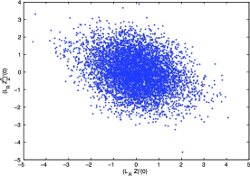
Figure 1: Scatter plot of $10\mbox{,}000$ random draws of $((L_{\mathbb{R}}{\mathbb{Z}})^{\prime}(0),(L_{\mathbb{R}}{\mathbb{Z}}_{2}^{0})^{\prime}(0))$ when $f(t_{0})=1$ and $f^{\prime}(t_{0})=-2$.

(v) We can show that the (unconditional) joint distribution of $(\Delta_{n}^{*},\mathbb{Z}_{n,2}^{0})$ converges to that of $((L_{\mathbb{R}}{\mathbb{Z}})^{\prime}(0),{\mathbb{Z}}_{2}^{0})$. But $\Delta_{n}^{*}$ and $\mathbb{Z}_{n,2}^{0}$ are asymptotically independent by Lemma 3.1 applied to $W_{n}=(\mathbb{Z}_{n,2}^{0}(t_{1}),\mathbb{Z}_{n,2}^{0}(t_{2}),\ldots,\mathbb{Z}_{n,2}^{0}(t_{l}))$, where $t_{i}\in\mathbb{R}$, $W_{n}^{*}=\Delta_{n}^{*}$ and $\mathcal{F}_{n}=\sigma(X_{1},X_{2},\ldots,X_{n})$. Therefore, $(L_{\mathbb{R}}{\mathbb{Z}})^{\prime}(0)$ and ${\mathbb{Z}}_{2}^{0}$ are independent. The proposition follows directly since $\mathbb{Z}_{2}$ is a measurable function of $\mathbb{Z}_{2}^{0}$.

If the conditional distribution of $\Delta^{*}_{n}$ converges in probability, as a consequence of (v) of Theorem 3.1, $(L_{\mathbb{R}}{\mathbb{Z}})^{\prime}(0)$ and $(L_{\mathbb{R}}{\mathbb{Z}}_{2}^{0})^{\prime}(0)$ must also be independent. Figure 1 shows the scatter plot of $(L_{\mathbb{R}}{\mathbb{Z}})^{\prime}(0)$ and $(L_{\mathbb{R}}{\mathbb{Z}}_{2}^{0})^{\prime}(0)$ obtained from a simulation study with $10\mbox{,}000$ samples, $f(t_{0})=1$ and $f^{\prime}(t_{0})=-2$. The correlation coefficient obtained $-0.2999$ is highly significant ($p$-value $<0.0001$). Thus, when combined with simulations, (v) of Theorem 3.1 strongly suggests that the conditional distribution of $\Delta_{n}^{*}$ does not converge in probability.

3.3 Bootstrapping from the EDF

A similar, slightly simpler pattern arises if the bootstrap sample is drawn from $\hat{F}_{n}={\mathbb{F}}_{n}$. Define ${\mathbb{Z}}_{n}^{*}$ as before, and let $\mathbb{Z}_{n,1}^{*}(h)=n^{2/3}\{(\mathbb{F}_{n}^{*}-{\mathbb{F}}_{n})(t_{0}+n^{-{1/3}}h)-(\mathbb{F}_{n}^{*}-{\mathbb{F}}_{n})(t_{0})\}$ and $\mathbb{Z}_{n,2}(h)=n^{2/3}\{{\mathbb{F}}_{n}(t_{0}+hn^{-{1/3}})-{\mathbb{F}}_{n}(t_{0})-\tilde{f}_{n}(t_{0})n^{-{1/3}}h\}$. Then ${\mathbb{Z}}_{n}^{*}={\mathbb{Z}}_{n,1}^{*}+{\mathbb{Z}}_{n,2}$. Recall the definition of the processes $\mathbb{W}_{1}$, $\mathbb{W}_{2}$, $\mathbb{Z}_{1}$, $\mathbb{Z}^{0}_{2}$ in Section 3.2. Define

$$\mathbb{Z}_{2}(h)=\mathbb{Z}_{2}^{0}(h)-(L_{\mathbb{R}}\mathbb{Z}_{2}^{0})^{\prime}(0)h.$$

Theorem 3.2

(i) The conditional distribution of $\mathbb{Z}_{n,1}^{*}$ given $\mathbf{X}=(X_{1},X_{2},\break\ldots)$ converges a.s. to the distribution of $\mathbb{Z}_{1}$.

[(iii)]

The unconditional distribution of $\mathbb{Z}_{n,2}$ converges to that of $\mathbb{Z}_{2}$ and the unconditional distributions of $(\mathbb{Z}_{n,1}^{*},\mathbb{Z}_{n,2})$, and $\mathbb{Z}_{n}^{*}$ converge to those of $(\mathbb{Z}_{1},\mathbb{Z}_{2})$ and $\mathbb{Z}$.

The unconditional distribution of $\Delta_{n}^{*}$ converges to that of $(L_{\mathbb{R}}\mathbb{Z})^{\prime}(0)$, and (15) fails.

Conditional on $\mathbf{X}$, the distribution of $\mathbb{Z}_{n}^{*}$ does not have a weak limit in probability.

If the conditional distribution function of $\Delta_{n}^{*}$ converges in probability, then $(L_{\mathbb{R}}{\mathbb{Z}})^{\prime}(0)$ and ${\mathbb{Z}}_{2}$ must be independent.

The proof of this theorem runs along similar lines to that of Theorem 3.1. We briefly highlight the differences.

The conditional convergence of $\mathbb{Z}_{n,1}^{*}$ follows from Proposition 2.1 with $m_{n}=n$, $F_{n}=\mathbb{F}_{n}$, $\mathbb{F}_{n,m_{n}}=\mathbb{F}_{n}^{*}$, applied conditionally given ${\mathbf{X}}$. It is only necessary to show that (4) is satisfied almost surely, and this follows from the Law of the Iterated Logarithm for ${\mathbb{F}}_{n}$, as explained in Section 2.3. Then the unconditional limiting distribution of $\mathbb{Z}_{n,1}^{*}$ must also be that of $\mathbb{Z}_{1}$.

The proof is similar to that of (ii) of Theorem 3.1, except that now $\mathbb{Z}_{n,2}(h)=\mathbb{Z}^{0}_{n,2}(h)-(L_{I_{n}}\mathbb{Z}^{0}_{n,2})^{\prime}(0)h$.

The proofs of (iii)–(v) are very similar to that of (iii)–(v) of Theorem 3.1.

3.4 Performance of the bootstrap methods in finite samples

In this subsection, we illustrate the poor finite sample performance of the two inconsistent bootstrap schemes, namely, bootstrapping from the EDF $\mathbb{F}_{n}$ and the NPMLE $\tilde{F}_{n}$. Table 1 shows the estimated coverage probabilities of nominal 95% confidence intervals for $f(1)$ using the two bootstrap methods

Table 1: Estimated coverage probabilities of nominal 95% confidence intervals for $f(1)$ while bootstrapping from the EDF $\mathbb{F}_{n}$ and NPMLE $\tilde{F}_{n}$, with varying sample size $n$ for the two models: $\operatorname{Exponential}(1)$ (left) and $|Z|$ where $Z\sim\operatorname{Normal}(0,1)$ (right)

$\bolds n$	EDF	NPMLE	$\bolds n$	EDF	NPMLE
$50$	0.747	0.720	0$50$	0.761	0.739
$100$	0.776	0.755	$100$	0.778	0.757
$200$	0.802	0.780	$200$	0.780	0.762
$500$	0.832	0.797	$500$	0.788	0.755

for different sample sizes, when the true distribution is assumed to be Exponential(1) and $|\mathrm{Normal}(0,1)|$, respectively. We used 1000 bootstrap samples to compute each confidence interval and then constructed 1000 such confidence intervals to estimate the actual coverage probabilities. As is clear from the table the coverage probabilities fall well short of the nominal 0.95 value. Leger and MacGibbon (2006) also illustrate such a discrepancy in the nominal and actual coverage probabilities while bootstrapping from the EDF for the Chernoff’s estimator of the mode.

Figure 2 shows the histograms (computed from 10,000 bootstrap samples) of the two inconsistent bootstrap distributions obtained from a single sample of 500 Exponential(1) random variables along with the histogram of the exact distribution of $\Delta_{n}$ (obtained from simulation). The bootstrap distributions are skewed and have very different shapes and supports compared to that on the left panel of Figure 2. The histograms illustrate the inconsistency of the bootstrap procedures.

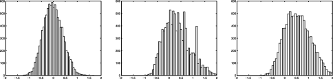
Figure 2: Histograms of the exact distribution of $\Delta_{n}$ (left panel) and the two bootstrap distributions while drawing bootstrap samples from $\mathbb{F}_{n}$ (middle panel) and $\tilde{F}_{n}$ (right panel) for $n=500$.

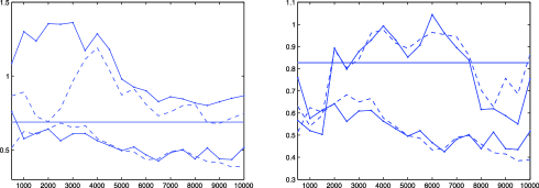
Figure 3: Estimated 0.95 quantile of the bootstrap distribution while generating the bootstrap samples from $\mathbb{F}_{n}$ (dashed lines) and $\tilde{F}_{n}$ (solid-dotted lines) for two independent data sequences along with the 0.95 quantile of the limit distribution of $\Delta_{n}$ (solid line) for the two models: $\operatorname{Exponential}(1)$ (left panel) and $|Z|$ where $Z\sim\operatorname{Normal}(0,1)$ (right panel).

The estimated coverage probabilities in Table 1 are unconditional [see (iii) of Theorems 3.1 and 3.2] and do not provide direct evidence to suggest that the conditional distribution of $\Delta_{n}^{*}$ does not converge in probability. Figure 3 shows the estimated 0.95 quantile of the bootstrap distribution for two independent data sequences as the sample size increases from 500 to 10,000, for the two bootstrap procedures, and for both the models (exponential and normal). The bootstrap quantile fluctuates enormously even at very large sample sizes and shows signs of nonconvergence. If the bootstrap were consistent, the estimated quantiles should converge to 0.6887 (0.8269), the 0.95 quantile of the limit distribution of $\Delta_{n}$, indicated by the solid line in Figure 3. From the left panel of Figure 3, we see that the estimated bootstrap 0.95 quantiles (obtained from the two procedures) for one data sequence stays below 0.6887, while for the other, the 0.95 quantiles stay above 0.6887, indicating the strong dependence on the sample path. Note that if the bootstrap distributions had a limit, then Figure 3 suggests that the limit varies with the sample path, and that is impossible as explained in Section 3.1. This provides evidence for the nonconvergence of the bootstrap estimator.

4 Consistent bootstrap methods

The main reason for the inconsistency of bootstrap methods discussed in the previous section is the lack of smoothness of the distribution function from which the bootstrap samples are generated. The EDF $\mathbb{F}_{n}$ does not have a density, and $\tilde{F}_{n}$ does not have a differentiable density, whereas $F$ is assumed to have a nonzero differentiable density at $t_{0}$. At a more technical level, the lack of smoothness manifests itself through the failure of (5).

The results from Section 2 may be directly applied to derive sufficient conditions on the smoothness of the distribution from which the bootstrap samples are generated. Let $X_{1},X_{2},\ldots\stackrel{{\scriptstyle\mathrm{ind}}}{{\sim}}F$; let $\hat{F}_{n}$ be an estimate of $F$ computed from $X_{1},\ldots,X_{n}$; and let $\hat{f}_{n}$ be the density of $\hat{F}_{n}$ or a surrogate, as in Section 3.

Theorem 4.1

If (2), (4), (5), (8) and (9) hold a.s. with $F_{n}=\hat{F}_{n}$ and $f_{n}=\hat{f}_{n}$, then the bootstrap estimate is strongly consistent, for example, (15) holds w.p. 1. In particular, the bootstrap estimate is strongly consistent if there is a $\delta>0$ for which $\hat{F}_{n}$ has a continuously differentiable density $\hat{f}_{n}$ on $[t_{0}-\delta,t_{0}+\delta]$, and (12) holds a.s. with $F_{n}=\hat{F}_{n}$ and $f_{n}=\hat{f}_{n}$.

That $\Delta_{n}^{*}$ converges weakly to the distribution on the right-hand side of (1) a.s. follows from Corollary 2.7 applied conditionally given $\mathbf{X}$ with $F_{n}=\hat{F}_{n}$ and $f_{n}=\hat{f}_{n}$. The second assertion follows similarly from Corollary 2.8.

4.1 Smoothing $\tilde{F}_{n}$

We show that generating bootstrap samples from a suitably smoothed version of $\tilde{F}_{n}$ leads to a consistent bootstrap procedure. To avoid boundary effects and ensure that the smoothed version has a decreasing density on $(0,\infty)$, we use a logarithmic transformation. Let $K$ be a twice continuously differentiable symmetric density for which

$$\int_{-\infty}^{\infty}[K(z)+|K^{\prime}(z)|+|K^{\prime\prime}(z)|]e^{\eta|z|}\,dz<\infty$$ (18)

for some $\eta>0$. Let

$$K_{h}(x,u) = {1\over hx}K\biggl{[}{1\over h}\log\biggl{(}{u\over x}\biggr{)}\biggr{]}\quad\mbox{and}$$

$$\check{f}_{n}(x) = \int_{0}^{\infty}K_{h}(x,u)\tilde{f}_{n}(u)\,du=\int_{0}^{\infty}K_{h}(1,u)\tilde{f}_{n}(xu)\,du.$$

Thus, $e^{y}\check{f}_{n}(e^{y})=\int_{-\infty}^{\infty}h^{-1}K[h^{-1}(y-z)]\tilde{f}_{n}(e^{z})e^{z}\,dz$. Integrating and using capital letters to denote distribution functions,

$$\check{F}_{n}(e^{y}) = \int_{-\infty}^{y}\check{f}_{n}(e^{s})e^{s}\,ds$$

$$= \int_{-\infty}^{y}\int_{-\infty}^{\infty}\frac{1}{h}K\biggl{(}\frac{s-v}{h}\biggr{)}\tilde{f}_{n}(e^{v})e^{v}\,dv\,ds$$

$$= \int_{-\infty}^{\infty}K(z)\tilde{F}_{n}(e^{y-hz})\,dz.$$

Alternatively, integrating (4.1) by parts yields

$$\check{f}_{n}(x)=-\int_{0}^{\infty}{\partial\over\partial u}K_{h}(x,u)\tilde{F}_{n}(u)\,du.$$

The proof of (15) requires showing that $\check{F}_{n}$ and its derivatives are sufficiently close to those of $F$, and it is convenient to separate the estimation error $\check{F}_{n}-F$ into sampling and approximation error. Thus, let

$$\bar{F}_{h}(e^{y})=\int_{-\infty}^{\infty}K(z)F(e^{y-hz})\,dz.$$ (20)

We denote the first and second derivatives of $\bar{F}_{h}$ by $\bar{f}_{h}$ and $\bar{f}_{h}^{\prime}$, respectively. Recall that $F$ is assumed to have a nonincreasing density on $(0,\infty)$ that is continuously differentiable near $t_{0}$.

Lemma 4.1

${\lim_{h\rightarrow 0}}\|\bar{F}_{h}-F\|=0$, and there is a $\delta>0$ for which

$$\lim_{h\to 0}\sup_{|x-t_{0}|\leq\delta}[|\bar{f}_{h}(x)-f(x)|+|\bar{f}_{h}^{\prime}(x)-f^{\prime}(x)|]=0.$$ (21)

First, observe that

$$\bar{F}_{h}(e^{y})-F(e^{y})=\int_{-\infty}^{\infty}K(z)[F(e^{y-hz})-F(e^{y})]\,dz$$

by (20). That $\lim_{h\rightarrow 0}\bar{F}_{h}(x)=F(x)$ for all $x\geq 0$ follows easily from the Dominated Convergence theorem, and uniform convergence then follows from Polya’s theorem. This establishes the first assertion of the lemma. Next, consider (21). Given $t_{0}>0$, let $y_{0}=\log(t_{0})$ and let $\delta>0$ be so small that $e^{y}f(e^{y})$ is continuously differentiable (in $y$) on $[y_{0}-2\delta,y_{0}+2\delta]$. Then

$$\bar{f}_{h}(x)-f(x) = \int_{-\infty}^{\infty}K(z)[f(xe^{hz})-f(x)]e^{hz}\,dz$$

$${}+f(x)\int_{-\infty}^{\infty}(e^{hz}-1)K(z)\,dz$$

and thus

$${\sup_{|x-t_{0}|\leq\delta}}|\bar{f}_{h}(x)-f(x)|\leq{\int_{-\infty}^{\infty}\sup_{|x-t_{0}|\leq\delta}}|f(xe^{hz})-f(x)|e^{hz}K(z)\,dz+O(h^{2})$$

for any $0<\delta<t_{0}$. For sufficiently small $\delta$, the integrand approach zero as $h\to 0$; and it is bounded by $\sup_{|x-t_{0}|\leq\delta}(e^{-hz}/x+f(x))e^{hz}K(z)$, since $f(x)\leq 1/x$ for all $x>0$. So the right-hand side approaches zero as $h\to 0$ by the Dominated Convergence theorem. That ${\sup_{|x-t_{0}|\leq\delta}}|\bar{f}_{h}^{\prime}(x)-f^{\prime}(x)|\to 0$ may be established similarly.

Theorem 4.2

Let $K$ be a twice continuously differentiable, symmetric density for which (18) holds. If

$$h=h_{n}\to 0\quad\mbox{and}\quad h_{n}^{2}\sqrt{n\over\log\log(n)}\to\infty,$$

then the bootstrap estimator is strongly consistent; that is, (15) holds a.s.

By Theorem 4.1, it suffices to show that (12) holds a.s. with $\hat{F}_{n}=\check{F}_{n}$ and $\hat{f}_{n}=\check{f}_{n}$; and this would follow from

$$\|\check{F}_{n}-\bar{F}_{h}\|+\sup_{|x-t_{0}|\leq\delta}[|\check{f}_{n}(x)-\bar{f}_{h}(x)|+|\check{f}_{n}^{\prime}(x)-\bar{f}_{h}^{\prime}(x)|]\rightarrow 0\qquad\mbox{a.s.}$$

for some $\delta>0$ and Lemma 4.1. Clearly, using (4.1),

$$\check{F}_{n}(e^{y})-\bar{F}_{h}(e^{y})=\frac{1}{h}\int_{-\infty}^{\infty}[\tilde{F}_{n}(e^{t})-F(e^{t})]K\biggl{(}\frac{y-t}{h}\biggr{)}\,dt$$ (22)

for all $y$, so that

$$\|\check{F}_{n}-\bar{F}_{h}\|\leq\|{\tilde{F}}_{n}-F\|\leq\|{\mathbb{F}}_{n}-F\|=O\bigl{[}\sqrt{\log\log(n)/n}\bigr{]}\qquad\mbox{a.s.}$$

by Marshall’s lemma and the Law of the Iterated Logarithm. Differentiating (22) gives

$$\check{f}_{n}(e^{y})-\bar{f}_{h}(e^{y})=\frac{e^{-y}}{h^{2}}\int_{-\infty}^{\infty}[\tilde{F}_{n}(e^{t})-F(e^{t})]K^{\prime}\biggl{(}\frac{y-t}{h}\biggr{)}\,dt.$$

Differentiating (22) again and then taking absolute values and considering $0<h\leq 1$, we get

$$\sup_{|x-t_{0}|\leq\delta}\{|\check{f}_{n}(x)-\bar{f}_{h}(x)|+|\check{f}_{n}^{\prime}(x)-\bar{f}_{h}^{\prime}(x)|\}$$

$$\qquad\leq\frac{M}{h^{3}}\sup_{|x-t_{0}|\leq\delta}\int_{-\infty}^{\infty}|\tilde{F}_{n}(e^{t})-F(e^{t})|\biggl{[}\biggl{|}K^{\prime}\biggl{(}\frac{\log x-t}{h}\biggr{)}\biggr{|}+\biggl{|}K^{\prime\prime}\biggl{(}\frac{\log x-t}{h}\biggr{)}\biggr{|}\biggr{]}\,dt$$

$$\qquad\leq\frac{M}{h^{2}}\|{\mathbb{F}}_{n}-F\|\int_{-\infty}^{\infty}[|K^{\prime}(z)|+|K^{\prime\prime}(z)|]\,dz\rightarrow 0\qquad\mbox{a.s.}$$

for a constant $M>0$, as $h_{n}^{2}\sqrt{n/\log\log(n)}\rightarrow\infty$, where Marshall’s lemma and the Law of Iterated Logarithm have been used again.

4.2 $m$ out of $n$ bootstrap

In Section 3, we showed that the two most intuitive methods of bootstrapping are inconsistent. In this section, we show that the corresponding $m$ out of $n$ bootstrap procedures are weakly consistent.

Theorem 4.3

If $\hat{F}_{n}=\mathbb{F}_{n}$, $\hat{f}_{n}=\tilde{f}_{n}$, and $m_{n}=o(n)$ then the bootstrap procedure is weakly consistent, for example, (15) holds in probability.

Conditions (2), (4) and (9) hold a.s. from (14), as explained in Section 2.3. To verify (8), let $\gamma>0$ be given. From the proof of Proposition 2.4 [also see Kim and Pollard (1990), page 218], there exists $\delta>0$ such that $|\mathbb{F}_{n}(t_{0}+h)-\mathbb{F}_{n}(t_{0})-F(t_{0}+h)-F(t_{0})|\leq\gamma h^{2}+\mathcal{C}_{n}n^{-2/3}$, for $|h|\leq\delta$, where $\mathcal{C}_{n}$’s are random variables of order $O_{P}(1)$. We can also assume that $|F(t_{0}+h)+F(t_{0})-f(t_{0})h-(1/2)f^{\prime}(t_{0})h^{2}|\leq(1/2)\gamma h^{2}$ for $|h|\leq\delta$. Then, using the inequality $2|ab|\leq\gamma a^{2}+b^{2}/\gamma$,

$$\biggl{|}\mathbb{F}_{n}(t_{0}+h)-\mathbb{F}_{n}(t_{0})-h\tilde{f}_{n}(t_{0})-\frac{1}{2}h^{2}f^{\prime}(t_{0})\biggr{|}$$

$$\qquad\leq\biggl{|}\mathbb{F}_{n}(t_{0}+h)-\mathbb{F}_{n}(t_{0})-hf(t_{0})-\frac{1}{2}h^{2}f^{\prime}(t_{0})\biggr{|}+|h||\tilde{f}_{n}(t_{0})-f(t_{0})|$$

$$\qquad\leq\biggl{\{}\gamma h^{2}+\mathcal{C}_{n}n^{-{2/3}}+\frac{1}{2}\gamma h^{2}\biggr{\}}+\biggl{\{}\frac{1}{2}\gamma h^{2}+\frac{1}{2\gamma}|\tilde{f}_{n}(t_{0})-f(t_{0})|^{2}\biggr{\}}$$

$$\qquad\leq 2\gamma h^{2}+\mathcal{C}_{n}n^{-{2/3}}+O_{P}(n^{-2/3})\leq 2\gamma h^{2}+o_{P}(m_{n}^{-{2/3}}).$$

For (5), write

$$m_{n}^{{2/3}}\{\mathbb{F}_{n}(t_{0}+m_{n}^{-{1/3}}h)-\mathbb{F}_{n}(t_{0})-m_{n}^{-{1/3}}\tilde{f}_{n}(t_{0})h\}$$

$$\qquad=m_{n}^{{2/3}}\{(\mathbb{F}_{n}-F)(t_{0}+m_{n}^{-{1/3}}h)-(\mathbb{F}_{n}-F)(t_{0})\}$$

(24)

$$\qquad\quad{}+m_{n}^{{1/3}}[f(t_{0})-\tilde{f}_{n}(t_{0})]h+\tfrac{1}{2}f^{\prime}(t_{0})h^{2}+o(1)$$

$$\qquad\stackrel{{\scriptstyle P}}{{\rightarrow}}\tfrac{1}{2}f^{\prime}(t_{0})h^{2}$$

uniformly on compacts using Hungarian Embedding to bound the second line and (1) (and a two-term Taylor expansion) in the third.

Given any subsequence $\{n_{k}\}\subset\mathbb{N}$, there exists a further subsequence $\{n_{k_{l}}\}$ such that (4.2) and (4.2) hold a.s. and Theorem 4.1 is applicable. Thus, (15) holds for the subsequence $\{n_{k_{l}}\}$, thereby showing that (15) holds in probability.

Next consider bootstrapping from $\tilde{F}_{n}$. We will assume slightly stronger conditions on $F$, namely, conditions (a)–(d) mentioned in Theorem 7.2.3 of Robertson, Wright and Dykstra (1988):

• $\alpha_{1}(F)=\inf\{x\dvtx F(x)=1\}<\infty$,

• $F$ is twice continuously differentiable on $(0,\alpha_{1}(F))$,

• $\gamma(F)=\frac{{\sup_{0<x<\alpha_{1}(F)}}|f^{\prime}(x)|}{\inf_{0<x<\alpha_{1}(F)}f^{2}(x)}<\infty$,

• $\beta(F)={\inf_{0<x<\alpha_{1}(F)}}|\frac{-f^{\prime}(x)}{f^{2}(x)}|>0$.

Theorem 4.4

Suppose that (a)–(d) hold. If $\hat{F}_{n}=\tilde{F}_{n}$, $\hat{f}_{n}=\tilde{f}_{n}$, and $m_{n}=o[n(\log n)^{-{3/2}}]$ then (15) holds in probability.

Conditions (2), (4) and (9) again follow from (14), as explained in Section 2.3. The verification of (8) is similar to the argument in the proof of Theorem 4.3. We show that (5) holds. Adding and subtracting $m_{n}^{{2/3}}[\mathbb{F}_{n}(t_{0}+m_{n}^{-{1/3}}h)-\mathbb{F}_{n}(t_{0})]$ from $\mathbb{Z}_{n,2}(h)$ and using (4.2) and the result of Kiefer and Wolfowitz (1976)

$$\sup_{|h|\leq c}\biggl{|}{\mathbb{Z}}_{n,2}(h)-{1\over 2}f^{\prime}(t_{0})h^{2}\biggr{|} \leq 2m_{n}^{2/3}\|\tilde{F}_{n}-{\mathbb{F}}_{n}\|+o_{P}(1)$$

$$\leq 2m_{n}^{2/3}\|\tilde{F}_{n}-{\mathbb{F}}_{n}\|+o_{P}(1)$$

$$= O_{P}[m_{n}^{2/3}n^{-{2/3}}\log(n)]+o_{P}(1)$$

for any $c>0$ from which (5) follows easily.

5 Discussion

We have shown that bootstrap estimators are inconsistent when bootstrap samples are drawn from either the EDF ${\mathbb{F}}_{n}$ or its least concave majorant ${\tilde{F}}_{n}$ but consistent when the bootstrap samples are drawn from a smoothed version of $\tilde{F}_{n}$ or an $m$ out of $n$ bootstrap is used. We have also derived necessary conditions for the bootstrap estimator to have a conditional weak limit, when bootstrapping from either ${\mathbb{F}}_{n}$ or ${\tilde{F}}_{n}$ and presented compelling numerical evidence that these conditions are not satisfied. While these results have been obtained for the Grenander estimator, our results and findings have broader implications for the (in)-consistency of the bootstrap methods in problems with an $n^{1/3}$ convergence rate.

To illustrate the broader implications, we contrast our finding with those of Abrevaya and Huang (2005), who considered a more general framework, as in Kim and Pollard (1990). For simplicity, we use the same notation as in Abrevaya and Huang (2005). Let $W_{n}:=r_{n}(\theta_{n}-\theta_{0})$ and $\hat{W}_{n}:=r_{n}(\hat{\theta}_{n}-\theta_{n})$ be the sample and bootstrap statistics of interest. In our case $r_{n}=n^{1/3}$, $\theta_{0}=f(t_{0})$, $\theta_{n}=\tilde{f}_{n}(t_{0})$ and $\hat{\theta}_{n}=\tilde{f}_{n}^{*}(t_{0})$. When specialized to the Grenander estimator, Theorem $2$ of Abrevaya and Huang (2005) would imply [by calculations similar to those in their Theorem 5 for the NPMLE in a binary choice model] that

$$\hat{W}_{n}\Rightarrow\arg\max\hat{Z}(t)-\arg\max Z(t)$$

conditional on the original sample, in $P^{\infty}$-probability, where $Z(t)=W(t)-ct^{2}$ and $\hat{Z}(t)=W(t)+\hat{W}(t)-ct^{2}$, $W$ and $\hat{W}$ are two independent two sided Brownian motions on $\mathbb{R}$ with $W(0)=\hat{W}(0)=0$ and $c$ is a positive constant depending on $F$. We also know that $W_{n}\Rightarrow\arg\max Z(t)$ unconditionally. By (v) of Theorem 3.1, this would force the independence of $\arg\max Z(t)$ and $\arg\max\hat{Z}(t)-\arg\max Z(t)$; but, there is overwhelming numerical evidence that these random variables are correlated.

Appendix

Lemma .1

Let $\Psi\dvtx\mathbb{R}\rightarrow\mathbb{R}$ be a function such that $\Psi(h)\leq M$ for all $h\in\mathbb{R}$, for some $M>0$, and

$$\lim_{|h|\rightarrow\infty}\frac{\Psi(h)}{|h|}=-\infty.$$ (25)

Then for any $b>0$, there exists $c_{0}>b$ such that for any $c\geq c_{0}$, $L_{\mathbb{R}}\Psi(h)=L_{[-c,c]}\Psi(h)$ for all $|h|\leq b$.

Note that for any $c>0$, $L_{\mathbb{R}}\Psi(h)\geq L_{[-c,c]}\Psi(h)$ for all $h\in[-c,c]$. Given $b>0$, consider $c>b$ and $\Phi_{c}(h)=L_{[-c,c]}\Psi(h)$ for $h\in[-b,b]$, and let $\Phi_{c}$ be the linear extension of $L_{[-c,c]}\Psi|_{[-b,b]}$ outside $[-b,b]$. We will show that there exists $c_{0}>b+1$ such that $\Phi_{c_{0}}\geq\Psi$. Then $\Phi_{c_{0}}$ will be a concave function everywhere greater than $\Psi$, and thus $\Phi_{c_{0}}\geq L_{\mathbb{R}}\Psi$. Hence, $L_{\mathbb{R}}\Psi(h)\leq\Phi_{c_{0}}(h)=L_{[-c_{0},c_{0}]}\Psi(h)$ for $h\in[-b,b]$, yielding the desired result.

For any $c>b+1$, $\Phi_{c}(h)=\Phi_{c}(b)-\Phi_{c}^{\prime}(b)+\Phi_{c}^{\prime}(b)(h-b+1)$ for $h\geq b$. Using the min–max formula,

$$\Phi_{c}^{\prime}(b) = \min_{-c\leq s\leq b}\max_{b\leq t\leq c}\frac{\Psi(t)-\Psi(s)}{t-s}$$

$$\geq \min_{-c\leq s\leq b}\frac{\Psi(b+1)-\Psi(s)}{(b+1)-s}$$

$$\geq \Psi(b+1)-M=:B_{0}\leq 0.$$

Thus,

$$\Phi_{c}(h) = \Phi_{c}(b)-\Phi_{c}^{\prime}(b)+\Phi_{c}^{\prime}(b)(h-b+1)$$

$$\geq \{\Psi(b)-\Phi_{c}^{\prime}(b)\}+\Phi_{c}^{\prime}(b)(h-b+1)$$

$$\geq \Psi(b)+(h-b)B_{0}$$

for $h\geq b+1$. Observe that $B_{0}$ does not depend on $c$. Combining this with a similar calculation for $h<-(b+1)$, there are $K_{0}\geq 0$ and $K_{1}\geq 0$, depending only on $b$, for which $\Phi_{c}(h)\geq K_{0}-K_{1}|h|$ for $|h|\geq b+1$. From (25), there is $c_{0}>b+1$ for which $\Psi(h)\leq K_{0}-K_{1}|h|$ for all $|h|\geq c_{0}$ in which case $\Psi(h)\leq\Phi_{c_{0}}(h)$ for all $h$. It follows that $L_{\mathbb{R}}\Psi\leq\Phi_{c_{0}}(h)$ for $|h|\leq b$.

Lemma .2

Let ${\mathbb{B}}$ be a standard Brownian motion. If $a,b,c>0,a^{3}b=1$, then

$$P\biggl{[}\sup_{t\in\mathbb{R}}{|{\mathbb{B}}(t)|\over a+bt^{2}}>c\biggr{]}=P\biggl{[}\sup_{s\in\mathbb{R}}{|{\mathbb{B}}(s)|\over 1+s^{2}}>c\biggr{]}.$$ (26)

This follows directly from rescaling properties of Brownian motion by letting $t=a^{2}s$. Proof of Proposition 2.4 Let $J=[a_{1},a_{2}]$ and $\varepsilon>0$ be as in the statement of the proposition; let $\gamma=|f^{\prime}(t_{0})|/16$; and recall (6) and (2.1) from the proof of Proposition 2.1. Then there exists $0<\delta<1$, $C\geq 1$, and $n_{0}\geq 1$ for which (8) and (9) hold for all $n\geq n_{0}$. Let $I_{m_{n}}^{*}:=[-\delta m_{n}^{1/3},\delta m_{n}^{1/3}]$. By making $\delta$ smaller, if necessary, and using Lemma 2.3, $L_{I_{m_{n}}}{\mathbb{Z}}_{n}(h)=L_{I_{m_{n}}^{*}}{\mathbb{Z}}_{n}(h)$ for $|h|\leq\delta m_{n}^{1/3}/2$ for all but a finite number of $n$ w.p. 1. By increasing the values of $C$ and $n_{0}$, if necessary, we may suppose that the right-hand side of (26) (with $c=C$) is less than $\varepsilon/3$, that $P[|\eta|>C]+P[\sup_{0\leq t\leq 1}m_{n}^{1/6}|{\mathbb{E}}_{m_{n}}(t)-{\mathbb{B}}_{m_{n}}^{0}(t)|>C]\leq\varepsilon/3$, and that $L_{I_{m_{n}}}{\mathbb{Z}}_{n}=L_{I_{m_{n}}^{*}}{\mathbb{Z}}_{n}$ on $[-{1\over 2}\delta m_{n}^{1/3},{1\over 2}\delta m_{n}^{1/3}]$ with probability at least $1-\varepsilon/3$ for all $n\geq n_{0}$. We can also assume that $\alpha:=8C^{3}/\gamma>1$. Then, using Lemma .2 with $a=\alpha m_{n}^{-{1/6}}$ and $b=a^{-3}$, the following relations hold simultaneously with probability at least $1-\varepsilon$ for $n\geq n_{0}$:

$$|{\mathbb{B}}_{m_{n}}[F_{n}(t_{0})+s]-{\mathbb{B}}_{m_{n}}[F_{n}(t_{0})]| \leq C\bigl{(}\alpha m_{n}^{-{1/6}}+\alpha^{-3}\sqrt{m_{n}}s^{2}\bigr{)}\qquad\mbox{for all }s,$$

$$L_{I_{m_{n}}}{\mathbb{Z}}_{n} = L_{I_{m_{n}}^{*}}{\mathbb{Z}}_{n}\qquad\mbox{on }\biggl{[}-\frac{\delta}{2}m_{n}^{1/3},\frac{\delta}{2}m_{n}^{1/3}\biggr{]},|\eta|\leq C,$$

and

$$\sup_{0\leq t\leq 1}m_{n}^{1/6}|{\mathbb{E}}_{m_{n}}(t)-{\mathbb{B}}_{m_{n}}^{0}(t)|\leq C.$$

Let $B_{n}$ be the event that these four conditions hold. Then $P(B_{n})\geq 1-\varepsilon$ for $n\geq n_{0}$, and from (2.1), $B_{n}$ implies

$$|{\mathbb{Z}}_{n,1}(h)| \leq C\{\alpha+\alpha^{-3}m_{n}^{2/3}[F_{n}(t_{0}+m_{n}^{-{1/3}}h)-F_{n}(t_{0})]^{2}\}+2C$$

$${}+Cm_{n}^{1/6}|F_{n}(t_{0}+m_{n}^{-{1/3}}h)-F_{n}(t_{0})|$$

$$\leq 4C\{\alpha+\alpha^{-1}m_{n}^{2/3}[F_{n}(t_{0}+m_{n}^{-{1/3}}h)-F_{n}(t_{0})]^{2}\}$$

using the inequalities $|F_{n}(t_{0}+m_{n}^{-{1/3}}h)-F_{n}(t_{0})|\leq\alpha m_{n}^{-{1/6}}+\alpha^{-1}m_{n}^{1/6}[F_{n}(t_{0}+m_{n}^{-{1/3}}h)-F_{n}(t_{0})]^{2}$ and $\alpha>1$. For sufficiently large $n$, using (9), we have

$$|\mathbb{Z}_{n,1}(h)| \leq 4C[\alpha+\alpha^{-1}C^{2}m_{n}^{2/3}(m_{n}^{-{1/3}}|h|+m_{n}^{-{1/3}})^{2}]$$

$$\leq 4C[\alpha+2\alpha^{-1}C^{2}(h^{2}+1)]$$

$$= \gamma h^{2}+\mathcal{C}$$

for $|h|\leq\delta m_{n}^{1/3}$ with $\mathcal{C}=4C\alpha+8C^{3}\alpha^{-1}$. Also, we can show that $|{\mathbb{Z}}_{n,2}(h)-f^{\prime}(t_{0})h^{2}/2|\leq\gamma h^{2}+\mathcal{C}$ for all $|h|\leq\delta m_{n}^{1/3}$ by (8). Let $b_{2}>a_{2}$ be such that $-5\gamma(a_{2}+b_{2})^{2}+6\gamma(a_{2}^{2}+b_{2}^{2})-8\mathcal{C}>0$.

Recalling that $\gamma=-f^{\prime}(t_{0})/16$, $B_{n}$ implies

$$-10\gamma h^{2}-2\mathcal{C}\leq{\mathbb{Z}}_{n}(h)={\mathbb{Z}}_{n,1}(h)+{\mathbb{Z}}_{n,2}(h)\leq-6\gamma h^{2}+2\mathcal{C}$$

for $|h|\leq\delta m_{n}^{1/3}$ and sufficiently large $n$. Since the right-hand side is concave, $B_{n}$ also implies $L_{I_{m_{n}}^{*}}{\mathbb{Z}}_{n}(h)\leq-6\gamma h^{2}+2\mathcal{C}$ for $|h|\leq\delta m_{n}^{1/3}$. Therefore, for sufficiently large $n$, using the upper bound on $L_{I_{m_{n}}^{*}}{\mathbb{Z}}_{n}$, the lower bound on $\mathbb{Z}_{n}$ obtained above, and $L_{I_{m_{n}}}{\mathbb{Z}}_{n}(h)=L_{I_{m_{n}}^{*}}{\mathbb{Z}}_{n}(h)$ for $|h|\leq\delta m_{n}^{1/3}/2$ on $B_{n}$, and $[a_{2},b_{2}]\subset I_{m_{n}}^{*}$, we have

$$2{\mathbb{Z}}_{n}\biggl{(}{a_{2}+b_{2}\over 2}\biggr{)}-[L_{I_{m_{n}}}{\mathbb{Z}}_{n}(a_{2})+L_{I_{m_{n}}}{\mathbb{Z}}_{n}(b_{2})]$$

$$\qquad\geq-5\gamma(a_{2}+b_{2})^{2}+6\gamma(a_{2}^{2}+b_{2}^{2})-8\mathcal{C}>0$$

with probability at least $1-\varepsilon$. Thus, $B_{n}$ implies $2{\mathbb{Z}}_{n}[{1\over 2}(a_{2}+b_{2})]>L_{I_{m_{n}}}{\mathbb{Z}}_{n}(a_{2})+L_{I_{m_{n}}}{\mathbb{Z}}_{n}(b_{2})$ with probability at least $1-\varepsilon$. Similarly, $B_{n}$ implies that there is a $b_{1}<a_{1}$ for which $2{\mathbb{Z}}_{n}[{1\over 2}(a_{1}+b_{1})]>L_{I_{m_{n}}}{\mathbb{Z}}_{n}(a_{1})+L_{I_{m_{n}}}{\mathbb{Z}}_{n}(b_{1})$ with probability at least $1-\varepsilon$. Relation (10) then follows from Lemma 2.2. It is worth noting as a remark that $b_{1},b_{2}$ do not depend on the sequence $F_{n}$.

Next, consider (11). Given a compact $J=[-b,b]$, let $c_{0}(\omega)$ be the smallest positive integer such that for any $c\geq c_{0}$, $L_{\mathbb{R}}\mathbb{Z}(h)=L_{[-c,c]}\mathbb{Z}(h)$ for $h\in J$. That $c_{0}$ exists and is finite w.p. 1 follows from Lemma .1. Defining $W_{c}:=L_{[-c,c]}\mathbb{Z}$ and $Y=L_{\mathbb{R}}\mathbb{Z}$, the event $\{W_{c}\neq Y\mbox{ on }J\}\subset\{c_{o}>c\}$. Now given any $\varepsilon>0$, there exist $c$ such that $P[c_{o}\leq c]>1-\varepsilon$. Therefore,

$$P\bigl{[}L_{\mathbb{R}}\mathbb{Z}=L_{[-c,c]}\mathbb{Z}\mbox{ on }J\bigr{]}\geq P[c_{o}\leq c]>1-\varepsilon.$$

Proof of Proposition 2.9 First, consider ${\mathbb{F}}_{n}$. Let $0<\gamma<|f^{\prime}(t_{0})|/2$ be given. There is a $0<\delta<{1\over 2}t_{0}$ such that

$$\bigl{|}F(t_{0}+h)-F(t_{0})-f(t_{0})h-\tfrac{1}{2}f^{\prime}(t_{0})h^{2}\bigr{|}\leq\tfrac{1}{2}\gamma h^{2}$$ (29)

for $|h|\leq 2\delta$. From the proof of Proposition 2.4, using arguments similar to deriving (Appendix) and (Appendix), we can show that

$$|({\mathbb{F}}_{n}-F)(t_{0}+h)-({\mathbb{F}}_{n}-F)(t_{0})|<\tfrac{1}{2}\gamma h^{2}+Cn^{-{2/3}}$$

for $|h|\leq 2\delta$ with probability at least $1-\varepsilon$ for sufficiently large $n$. Therefore, by adding and subtracting $F(t_{0}+h)-F(t_{0})$ and using (29),

$$\bigl{|}{\mathbb{F}}_{n}(t_{0}+h)-{\mathbb{F}}_{n}(t_{0})-f(t_{0})h-\tfrac{1}{2}f^{\prime}(t_{0})h^{2}\bigr{|}\leq\gamma h^{2}+Cn^{-{2/3}}$$ (30)

for $|h|\leq 2\delta$ with probability at least $1-\varepsilon$ for large $n$.

Next, consider $\tilde{F}_{n}$. Let $B_{n}$ denote the event that (30) holds. Then $P(B_{n})$ is eventually larger than $1-\varepsilon$ and on $B_{n}$, we have

$${\mathbb{F}}_{n}(t_{0}+h)-\mathbb{F}_{n}(t_{0})-f(t_{0})h\leq\bigl{\{}\gamma-\tfrac{1}{2}|f^{\prime}(t_{0})|\bigr{\}}h^{2}+Cn^{-{2/3}}$$

for $|h|\leq 2\delta$. Let $E_{n}$ be the event that $\tilde{F}_{n}(h)=L_{[t_{0}-2\delta,t_{0}+2\delta]}{\mathbb{F}}_{n}(h)$ for $h\in[t_{0}-\delta,t_{0}+\delta]$. Then by Lemma 2.3, $P(E_{n})\geq 1-\varepsilon$, for all sufficiently large $n$. Taking concave majorants on either side of the above display for $|h|\leq 2\delta$ and noting that the right-hand side of the display is already concave, we have: ${\tilde{F}}_{n}(t_{0}+h)-\mathbb{F}_{n}(t_{0})-f(t_{0})h\leq\{\gamma-\frac{1}{2}|f^{\prime}(t_{0})|\}h^{2}+Cn^{-{2/3}}$, for $|h|\leq\delta$ on $B_{n}\cap E_{n}$. Setting $h=0$ shows that on $E_{n}\cap B_{n}$, $\tilde{F}_{n}(t_{0})-\mathbb{F}_{n}(t_{0})\leq Cn^{-{2/3}}$. Now, as ${\mathbb{F}}_{n}(t_{0})\leq\tilde{F}_{n}(t_{0})$, it is also the case that on $E_{n}\cap B_{n}$, for $|h|\leq\delta$,

$${\tilde{F}}_{n}(t_{0}+h)-\tilde{F}_{n}(t_{0})-f(t_{0})h\leq\bigl{\{}\gamma-\tfrac{1}{2}|f^{\prime}(t_{0})|\bigr{\}}h^{2}+Cn^{-{2/3}}.$$ (31)

Furthermore on $E_{n}\cap B_{n}$,

$$\tilde{F}_{n}(t_{0}+h)-\tilde{F}_{n}(t_{0})-f(t_{0})h-\tfrac{1}{2}f^{\prime}(t_{0})h^{2}$$

$$\qquad\geq\mathbb{F}_{n}(t_{0}+h)-\{\mathbb{F}_{n}(t_{0})+Cn^{-{2/3}}\}-f(t_{0})h-\tfrac{1}{2}f^{\prime}(t_{0})h^{2}$$ (32)

$$\qquad\geq-\gamma h^{2}-2Cn^{-{2/3}}.$$

Therefore, combining (31) and (Appendix),

$$\bigl{|}{\tilde{F}}_{n}(t_{0}+h)-{\tilde{F}}_{n}(t_{0})-f(t_{0})h-\tfrac{1}{2}f^{\prime}(t_{0})h^{2}\bigr{|}\leq\gamma h^{2}+2Cn^{-{2/3}}$$

for $|h|\leq\delta$ with probability at least $1-2\varepsilon$ for large $n$.

References

- (1) Abrevaya, J. and Huang, J. (2005). On the bootstrap of the maximum score estimator. Econometrica 73 1175–1204. \MR2149245
- (2) Andrews, D. F., Bickel, P. J., Hampel, F. R., Huber, P. J., Rogers, W. H. and Tukey, J. W. (1972). Robust Estimates of Location. Princeton Univ. Press, Princeton, NJ. \MR0331595
- (3) Bickel, P. and Freedman, D. (1981). Some asymptotic theory for the bootstrap. Ann. Statist. 9 1196–1217. \MR0630103
- (4) Breiman, L. (1968). Probability. Addison-Wesley, Reading, MA. \MR0229267
- (5) Brunk, H. D. (1970). Estimation of isotonic regression. In Nonparametric Techniques in Statistical Inference (M. L. Puri, ed.) 177–197. Cambridge Univ. Press, London. \MR0277070
- (6) Chernoff, H. (1964). Estimation of the mode. Ann. Inst. Statist. Math. 16 31–41. \MR0172382
- (7) Grenander, U. (1956). On the theory of mortality measurement. Part II. Skand. Aktuarietidskr. 39 125–153. \MR0093415
- (8) Groeneboom, P. (1985). Estimating a monotone density. In Proceedings of the Berkeley Conference in Honor of Jerzy Neyman and Jack Kiefer (L. M. Le Cam and R. A. Olshen, eds.) 2 539–554. IMS, Hayward, CA. \MR0822052
- (9) Groeneboom, P. and Wellner, J. A. (2001). Computing Chernoff’s distribution. J. Comput. Graph. Statist. 10 388–400. \MR1939706
- (10) Kiefer, J. and Wolfowitz, J. (1976). Asymptotically minimax estimation of concave and convex distribution functions. Z. Wahrsch. Verw. Gebiete 34 73–85. \MR0397974
- (11) Kim, J. and Pollard, D. (1990). Cube-root asymptotics. Ann. Statist. 18 191–219. \MR1041391
- (12) Kómlos, J., Major, P. and Tusnády, G. (1975). An approximation of partial sums of independent RV’s and the sample DF.I. Z. Wahrsch. Verw. Gebiete 32 111–131. \MR0375412
- (13) Kosorok, M. (2008). Bootstrapping the Grenander estimator. In Beyond Parametrics in Interdisciplinary Research: Festschrift in Honour of Professor Pranab K. Sen (N. Balakrishnan, E. Pena and M. Silvapulle, eds.) 282–292. IMS, Beachwood, OH. \MR2462212
- (14) Lee, S. M. S. and Pun, M. C. (2006). On out of bootstrapping for nonstandard M-estimation with nuisance parameters. J. Amer. Statist. Assoc. 101 1185–1197. \MR2328306
- (15) Léger, C. and MacGibbon, B. (2006). On the bootstrap in cube root asymptotics. Canad. J. Statist. 34 29–44. \MR2267708
- (16) Loève, M. (1963). Probability Theory. Van Nostrand, Princeton. \MR0203748
- (17) Politis, D. N., Romano, J. P. and Wolf, M. (1999). Subsampling. Springer, New York. \MR1707286
- (18) Pollard, D. (1984). Convergence of Stochastic Processes. Springer, New York. Available at http://www.stat.yale.edu/~pollard/1984book/pollard1984.pdf. \MR0762984
- (19) Prakasa Rao, B. L. S. (1969). Estimation of a unimodal density. Sankhāya Ser. A 31 23–36. \MR0267677
- (20) Robertson, T., Wright, F. T. and Dykstra, R. L. (1988). Order Restricted Statistical Inference. Wiley, New York. \MR0961262
- (21) Rousseeuw, P. J. (1984). Least median of squares regression. J. Amer. Statist. Assoc. 79 871–880. \MR0770281
- (22) Shao, J. and Tu, D. (1995). The Jackknife and Bootstrap. Springer, New York. \MR1351010
- (23) Shorack, G. R. and Wellner, J. A. (1986). Empirical Processes with Applications to Statistics. Wiley, New York. \MR0838963
- (24) Singh, K. (1981). On asymptotic accuracy of Efron’s bootstrap. Ann. Statist. 9 1187–1195. \MR0630102
- (25) van der Vaart, A. W. and Wellner, J. A. (2000). Weak Convergence and Empirical Processes. Springer, New York.
- (26) Wang, X. and Woodroofe, M. (2007). A Kiefer Wolfowitz comparison theorem for Wicksell’s problem. Ann. Statist. 35 1559–1575. \MR2351097