Electron Wave Function in Armchair Graphene Nanoribbons

Abstract

By using analytical solution of a tight-binding model for armchair nanoribbons, it is confirmed that the solution represents the standing wave formed by intervalley scattering and that pseudospin is invariant under the scattering. The phase space of armchair nanoribbon which includes a single Dirac singularity is specified. By examining the effects of boundary perturbations on the wave function, we suggest that the existance of a strong boundary potential is inconsistent with the observation in a recent scanning tunneling microscopy. Some of the possible electron-density superstructure patterns near a step armchair edge located on top of graphite are presented. It is demonstrated that a selection rule for the G band in Raman spectroscopy can be most easily reproduced with the analytical solution.

1 Introduction

Graphene nanoribbons are particularly useful in studying the properties which are hidden in carbon nanotubes by the periodic boundary condition. [1] The boundary of a nanoribbon consists of two symmetrical edge structures, armchair and zigzag edges. A transmission electron microscope image illustrates that the edge of a sample prepared by micromechanical cleavage, [2] is a mixture of armchair and zigzag edges. [3] Some attempts have been made to prepare a regular zigzag or armchair edge over a large length more than 20 nm. [4]

It is known that the behavior of the electrons near zigzag edge differs greatly from that near armchair edge in many respects. For example, armchair edge gives rise to intervalley scattering, while zigzag edge produces intravalley scattering. This originates from the fact that the graphene Brillouin zone in the $k$-space is given by rotating the hexagonal unit cell in real space by 90^∘. [5] On the other hand, zigzag edge changes the orientation of pseudospin, while armchair edge does not. This behavior of pseudospin results from that only A or B (both A and B) sublattice appears at zigzag (armchair) edge. These differences between zigzag and armchair edges cause observable effects to appear in Raman spectra. Because the D band in Raman spectra is relevant to intervalley scattering, it follows that the D band intensity is enhanced by armchair edge. [6] The behavior of pseudospin is essential to a selection rule of the G band for the graphene edge. [7]

Besides the differences in the behavior of the scattering and pseudospin, armchair and zigzag edges are distinct with respect to the number of Dirac singularities. In the case of nanotube, there are two Dirac singularities corresponding to the K and K^′ points at the corners of the first Brillouin zone. By means of an effective-mass theory, we discussed in a previous paper that there is a single Dirac singularity in the phase space of armchair nanoribbon, while there is no Dirac singularity in the phase space of the standing wave of zigzag nanoribbon. [5] The existence of a single Dirac singularity in armchair nanoribbon is of particular interest in transport property because the existence of the Dirac singularity can suppress backward scattering. The appearance of the edge states [8, 9] near zigzag edge is a consequence of the absence of the Dirac singularity for zigzag nanoribbon.

In this paper, by constructing analytical solution of a tight-binding model for armchair nanoribbons, we account for the features of armchair edge, such as intervalley scattering, the behavior of pseudospin, and the single Dirac singularity in the phase space. Since the tight-binding model has an atomic resolution, we can apply the solution to some recent experimental results obtained by scanning tunneling microscopy. [10, 11]

Here, we would like to mention the previously published literature on analytical solution for the wave function in armchair nanoribbon. Compernolle et al. [12] constructed the wave functions in nanoribbons (achiral nanotubes with edges) using the transfer matrix method. They applied the result to obtain the transmission coefficient. Zheng et al. [13] conducted analytical study of electronic state in armchair nanoribbons. They showed that all armchair nanoribbons acquire nonzero energy gap due to the variation of hopping integral near the edges. The above-mentioned authors employed a simple nearest-neighbor tight-binding Hamiltonian that was shown to be a good approximation for describing the electrons in nanotubes and graphene systems. In this paper, we use the same Hamiltonian to examine armchair nanoribbons.

This paper is organized as follows. In §2 we solve a simple tight-binding model for armchair nanoribbons, and obtain the energy dispersion eq. (13) and the wave function eq. (24). The characteristic features of the wave function are pointed out. By using eq. (24) we will show in §3.1 that a feature of the Dirac singularity for armchair edge has been observed in recent scanning tunneling microscopy experiment by Yang et al. [10], and in §3.2 that the electron-phonon matrix element for the G band in Raman spectra which we have derived numerically with a tight-binding model in a previous paper [14] can be derived analytically. Discussion and summary are given in §4.

2 Construction of Wave Function

Let $\phi_{A}^{J}$ and $\phi_{B}^{J}$ be the probability amplitudes of the A and B-atoms at the box in $J$th line shown in Fig. 1(a), then the Schrödinger equation for the electron in an armchair nanoribbon is written as the recurrence equation,

$$-\epsilon\begin{pmatrix}\phi_{A}^{J}\cr\phi_{B}^{J}\end{pmatrix}= \begin{pmatrix}0&1\cr 1&0\end{pmatrix}\begin{pmatrix}\phi_{A}^{J}\cr\phi_{B}^{J}\end{pmatrix}+\begin{pmatrix}0&e^{-ikb}\cr 1&0\end{pmatrix}\begin{pmatrix}\phi_{A}^{J-1}\cr\phi_{B}^{J-1}\end{pmatrix}$$

$$+\begin{pmatrix}0&1\cr e^{+ikb}&0\end{pmatrix}\begin{pmatrix}\phi_{A}^{J+1}\cr\phi_{B}^{J+1}\end{pmatrix}.$$ (1)

Here, $\epsilon$ is the energy eigenvalue in units of the hopping integral ($\gamma=3$ eV), $k$ is the wave vector along the edge, and $b$ ($\equiv 2l$) denotes the unit length along the axis of armchair nanoribbon [see Fig. 1(a)]. In obtaining eq. (1) we have used the Bloch theorem, by which the amplitude of the B-atom in $J-1$th line that is located nearest to the A-atom at the box in $J$th line is given by $e^{-ikb}\phi_{B}^{J-1}$. Note that $J$ in eq. (1) takes from $J=2$ to $N-1$. For $J=1$ and $J=N$, the recurrence equations are given by

$$-\epsilon\begin{pmatrix}\phi_{A}^{1}\cr\phi_{B}^{1}\end{pmatrix}=\begin{pmatrix}0&1\cr 1&0\end{pmatrix}\begin{pmatrix}\phi_{A}^{1}\cr\phi_{B}^{1}\end{pmatrix}+\begin{pmatrix}0&1\cr e^{+ika}&0\end{pmatrix}\begin{pmatrix}\phi_{A}^{2}\cr\phi_{B}^{2}\end{pmatrix},$$ (2)

$$-\epsilon\begin{pmatrix}\phi_{A}^{N}\cr\phi_{B}^{N}\end{pmatrix}=\begin{pmatrix}0&1\cr 1&0\end{pmatrix}\begin{pmatrix}\phi_{A}^{N}\cr\phi_{B}^{N}\end{pmatrix}+\begin{pmatrix}0&e^{-ikb}\cr 1&0\end{pmatrix}\begin{pmatrix}\phi_{A}^{N-1}\cr\phi_{B}^{N-1}\end{pmatrix}.$$ (3)

When we assume that eq. (1) is satisfied for $J=1,\cdots,N$, these equations at $J=1$ and $J=N$ can be included as the boundary condition;

$$\begin{pmatrix}\phi^{0}_{A}\cr\phi^{0}_{B}\end{pmatrix}=0,\ \ \begin{pmatrix}\phi^{N+1}_{A}\cr\phi^{N+1}_{B}\end{pmatrix}=0.$$ (4)

In the following, we solve the recurrence equation of eq. (1) with the boundary condition of eq. (4).

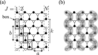
Figure 1: (a) The structure of an armchair graphene nanoribbon. The index $J$ takes from $1$ to $N$. The lattice constant is $a$ ($=\sqrt{3}a_{\rm cc}$). The unit length and the wave vector along the axis are denoted by $b$ ($=3a_{\rm cc}$) and $k$, respectively. Carbon atoms are divided into A ($\bullet$) and B ($\circ$) atoms. (b) The electron-density pattern of the Dirac singularity state in a metallic armchair nanoribbon with $N=8$. See also the STM topography shown in Fig. 3 of Ref. yang10.

First, let us introduce the following matrices,

$$K=\begin{pmatrix}\epsilon&1\cr 1&\epsilon\end{pmatrix},\ \ T=\begin{pmatrix}0&1\cr z&0\end{pmatrix},\ \ T^{-1}=\begin{pmatrix}0&z^{*}\cr 1&0\end{pmatrix},$$ (5)

where $z=e^{+ikb}$, $z^{*}=e^{-ikb}$, and $kb\in[-\pi,\pi)$. Then eq. (1) is rewritten as

$$T\phi^{J+1}+K\phi^{J}+T^{-1}\phi^{J-1} =0,\ \ (J=1,\cdots,N)$$ (6)

where we have defined $\phi^{J}\equiv{}^{t}(\phi^{J}_{A},\phi^{J}_{B})$. By multiplying eq. (6) by $T^{-1}$ from the left-hand side, we get $\phi^{J+1}+T^{-1}K\phi^{J}+(T^{-1})^{2}\phi^{J-1}=0$. Because the matrix $T^{-1}$ satisfies $(T^{-1})^{2}=z^{*}\sigma_{0}$, where $\sigma_{0}$ is $2\times 2$ identity matrix, the recurrence equation can be diagonalized by some matrix $U$ as

$$\varphi^{J+1}+U^{-1}T^{-1}KU\varphi^{J}+\frac{1}{z}\varphi^{J-1}=0,$$ (7)

where $\varphi^{J}\equiv U^{-1}\phi^{J}$. It is straightforward to show that the eigenvalues of the matrix $T^{-1}K$ are given by

$$\lambda_{\pm}=\frac{1+z\pm\sqrt{(-1+z)^{2}+4z\epsilon^{2}}}{2z},$$ (8)

and the corresponding eigen spinors are

$$\phi_{\pm}=\begin{pmatrix}\frac{1-z\pm\sqrt{(-1+z)^{2}+4z\epsilon^{2}}}{2z\epsilon}\cr 1\end{pmatrix}.$$ (9)

The eigenvalue $\lambda_{+}$ (or $\lambda_{-}$) is a multivalued function since $\sqrt{z}$ has two branches:

$$w_{+}=+e^{ikl},\ \ w_{-}=-e^{ikl}.$$ (10)

The eigenvalue $\lambda_{+}$ with the $w_{+}$ ($w_{-}$) branch is equivalent to the eigenvalue $\lambda_{-}$ with the $w_{-}$ ($w_{+}$) branch. As a result, we may consider the eigenvalue $\lambda_{+}$ only. Here we consider the $w_{+}$ branch. We will show later that the $w_{-}$ branch gives the same wave function as the $w_{+}$ branch, and that these $w_{+}$ and $w_{-}$ branches correspond to different states in the case of carbon nanotubes.

Next, we solve the characteristic equation with respect to eq. (7) as

$$x^{2}+\lambda_{+}x+\frac{1}{z}=0$$

$$\leftrightarrow\left(x-w_{+}^{-1}e^{+i\theta}\right)\left(x-w_{+}^{-1}e^{-i\theta}\right)=0,$$ (11)

where the parameter $\theta\in(0,\pi)$ is defined by $2\cos\theta\equiv-w_{+}\lambda_{+}$ or

$$2\cos\theta\equiv-\frac{w_{+}^{-1}+w_{+}+\sqrt{z+z^{*}-2+4\epsilon^{2}}}{2}.$$ (12)

The solution to the characteristic equation is given by $x=w_{+}^{-1}e^{+i\theta}$ or $x=w_{+}^{-1}e^{-i\theta}$. Since $w_{+}^{-1}+w_{+}=2\cos(kl)$ and $z+z^{*}=2\cos(2kl)$, eq. (12) leads to the energy dispersion relation,

$$\epsilon^{2}=1+4\cos^{2}\theta+4\cos\theta\cos(kl).$$ (13)

By employing the standard method for solving the recurrence equation, general $J$th term is written by the first and second terms, $\phi^{1}_{+}$ and $\phi^{2}_{+}$, as

$$\phi_{+}^{J}=w_{+}^{-(J-2)}\frac{\sin(J-1)\theta}{\sin\theta}\phi^{2}_{+}-w_{+}^{-(J-1)}\frac{\sin(J-2)\theta}{\sin\theta}\phi^{1}_{+}.$$ (14)

To this point, we have not yet used the boundary condition. The remaining procedure for obtaining the solution is applying the boundary condition to eq. (14). The boundary condition of armchair edge is given by $\phi^{0}=0$. Thus, eq. (7) with $J=1$ gives $\phi^{2}=-T^{-1}K\phi^{1}$, so that we have

$$\phi^{2}_{+}=-\lambda_{+}\phi^{1}_{+}=\frac{2\cos\theta}{w_{+}}\phi^{1}_{+}.$$ (15)

By putting this into eq. (14), we obtain

$$\phi^{J}_{+}=w_{+}^{-(J-1)}\frac{\sin J\theta}{\sin\theta}\phi^{1}_{+}.$$ (16)

The eigen spinor $\phi_{+}^{1}$ may be represented in a simpler fashion as

$$\phi^{1}_{+}=\begin{pmatrix}1+\frac{2\cos\theta}{w_{+}}\cr-\epsilon\end{pmatrix}=|\epsilon|\begin{pmatrix}e^{-i\Theta}\cr-s\end{pmatrix},$$ (17)

where the variable $\Theta$ is a function of $k$ and $\theta$, and $s$ takes $+1$ ($-1$) for a conduction (valence) band state [$\epsilon=s|\epsilon|$]. Therefore, the wave function is written as

$$\phi^{J}_{+}(s,k,\theta)=Ce^{-ikl(J-1)}\frac{\sin J\theta}{\sin\theta}\begin{pmatrix}e^{-i\Theta(k,\theta)}\cr-s\end{pmatrix},$$ (18)

where $C$ is the normalization constant.

Several characteristic features of armchair nanoribbons can be derived from the wave function eq. (18) and energy dispersion relation eq. (13). They are listed as follows.

(I) Armchair nanoribbons are metallic for the case that $N=3i-1$, [15, 16, 17] where $i$ is integer. From the energy dispersion relation of eq. (13) one can see that the state with $\epsilon=0$ corresponds to the point $(0,2\pi/3)$ in the parameter space $(k,\theta)$. The parameter $\theta$ is quantized as $\theta_{n}=n\pi/(N+1)$ [$n=1,\cdots,N$] by imposing the boundary condition on the wave function: $\phi^{N+1}_{+}(s,k,\theta)=0$. The quantized parameter $\theta_{n}$ takes $2\pi/3$ for the case that $N=3i-1$ and $n=2i$.

(II) The angle $\Theta(k,\theta)$ in eq. (18) is singular at the point $(0,2\pi/3)$. By putting $(\delta k,2\pi/3+\delta\theta)$ into $1+2\cos\theta/w_{+}$ of eq. (17), we have $|\epsilon|e^{-i\Theta}=(-\sqrt{3}\delta\theta+i\delta kl)$ and $|\epsilon|=\sqrt{3\delta\theta^{2}+(\delta kl)^{2}}$. The parameter $\Theta$ changes from $0$ to $2\pi$ when $(\delta k,\delta\theta)$ moves along a path enclosing the singularity point. This behavior of $\Theta$ results in a nontrivial Berry’ phase which is a necessary condition for an armchair nanoribbon to exhibit a ballistic transport. [18, 5]

(III) The wave function can be understood as the standing wave formed by intervalley scattering. This feature can be made more transparent by rewriting $\sin(J\theta)$ of eq. (24) in terms of exponential functions as

$$\phi^{J}_{+}(s,k,\theta)\propto e^{-iklJ}\left[e^{+iJ\theta}\begin{pmatrix}e^{-i\Theta}\cr-s\end{pmatrix}-e^{-iJ\theta}\begin{pmatrix}e^{-i\Theta}\cr-s\end{pmatrix}\right],$$ (19)

where the parameter $\theta\in(0,\pi)$ is a positive value. The exponential function $e^{+iJ\theta}$ ($e^{-iJ\theta}$) indicates the propagating wave in the direction of increasing (decreasing) $J$. Hence, for the armchair edge at $J=1$, the second term represents the incident wave to the edge and the first term represents the reflected wave. The momentum transfer through this scattering process, $-\theta\to\theta$, is given by $2\theta$. Since $\theta=2\pi/3$ ($\equiv\theta_{\rm F}$) is coincident with $k_{\rm F}a/2$, where $k_{\rm F}$ is the wave vector at the K point, we can see that the change in the wave vector at the armchair edge is given by $2\theta_{\rm F}=k_{\rm F}a$. This change of the wave vector corresponds to the intervalley scattering.

(IV) The spinors of the incident and edge reflected waves in eq. (19) are equal. Hence, the pseudospin does not change under the intervalley scattering at armchair edge. This feature originates from the fact that both the A and B-atoms appear equivalently at the armchair edge. It is also clear that the probability densities at the A and B-atoms in $J$th line are equal and the electron-density pattern depends only on the distance from the armchair edge.

(V) There is a single Dirac singularity in the system. To make this point clear, we rewrite the standing wave eq. (19) as

$$\phi^{J}_{+}=\psi_{\rm K}-\psi_{\rm K^{\prime}},$$ (20)

where $\psi_{\rm K}$ ($\psi_{\rm K^{\prime}}$) corresponds to a Bloch state near the K (K^′) point. The minus sign in front of $\psi_{\rm K^{\prime}}$ shows that this standing wave is an anti-symmetric combination of the two Bloch states. If the two states were independent of each other, we may expect that the symmetric combination $\psi_{\rm K}+\psi_{\rm K^{\prime}}$ is also a solution. However, such symmetric solution should be excluded because $\psi_{\rm K}+\psi_{\rm K^{\prime}}$ is proportional to $\cos(J\theta)$ and does not satisfy the armchair boundary condition. Since the armchair boundary condition selects only the antisymmetric solution, the two Dirac points (K and K^′) are no longer independent of each other in armchair nanoribbon. Therefore, the number of Dirac singularities is reduced to one in this system. On the other hand, the two Dirac points (K and K^′) are independent of each other in the case of nanotube because the symmetric and antisymmetric combinations can satisfy the periodic boundary condition of nanotube.

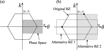
Figure 2: (a) The region denoted by shadow, $\theta\in(0,\pi)$ and $k\in[-\pi/b,\pi/b)$, represents the phase space of armchair nanoribbon. The empty circle indicates the position of the Dirac singularity. (b) Two alternative Brillouin zones (BZ 1 and BZ 2) for graphene. The BZ 1 is useful to understand that the phase space of armchair nanoribbon is given by folding BZ 1 into the positive region of $\theta$ with respect to the $k$-axis. The shadow region (BZ 2) is used to discuss on the Riemann sheets (see text). Note that alternative BZs contain two singularities corresponding to the K and K^′ points, while the phase space of armchair nanoribbon has a single singularity.

(VI) The phase space of armchair nanoribbon is given by $\theta\in(0,\pi)$ and $k\in[-\pi/b,\pi/b)$ [See Fig. 2(a)]. By comparing the phase space of armchair nanoribbon with the usual hexagonal Brillouin zone (BZ) of graphene, it can be seen that the former covers only the half region of the latter. To explore this feature further, we consider the other branch $w_{-}$. Repeating analysis similar to that above, we obtain the corresponding energy dispersion relation and the wave function as

$$\epsilon^{2}=1+4\cos^{2}\theta^{\prime}-4\cos\theta^{\prime}\cos(kl),$$ (21)

$$\phi^{J}_{-}=w_{-}^{-(J-1)}\frac{\sin(J\theta^{\prime})}{\sin\theta^{\prime}}\begin{pmatrix}1+\frac{2\cos\theta^{\prime}}{w_{-}}\cr-\epsilon\end{pmatrix},$$ (22)

where $\theta^{\prime}\in(-\pi,0)$ is defined by

$$2\cos\theta^{\prime}\equiv-\frac{w_{-}^{-1}+w_{-}+\sqrt{z+z^{*}-2+4\epsilon^{2}}}{2}.$$ (23)

By subtracting eq. (23) from eq. (12), we get $\cos\theta^{\prime}=\cos\theta+\cos(kl)$. Using this relationship between $\theta$ and $\theta^{\prime}$, we see that the point $(k,\theta)=(0,2\pi/3)$ corresponds to $\theta^{\prime}=-\pi/3$, for which $\phi^{J}_{-}$ reproduces $\phi^{J}_{+}$. Generally, by setting $\theta^{\prime}=\theta-\pi$ in eq. (22), we obtain the wave function $\phi^{J}_{+}$ of eq. (16). Thus, the $w_{-}$ branch does not yield a state which is independent of the $w_{+}$ branch. Hence, we may consider the $w_{+}$ branch only. This observation allows us to interpret the phase space of armchair nanoribbon shown in Fig. 2(a) as the region given by holding the alternative BZ 1 of nanotube shown in Fig. 2(b) into the positive region of $\theta$. In the remainder of the paper, we abbreviate $\phi^{J}_{\pm}(s,k,\theta)$ as $\phi^{J}_{s}(k,\theta)$,

$$\phi^{J}_{s}(k,\theta)=Ce^{-ikl(J-1)}\frac{\sin J\theta}{\sin\theta}\begin{pmatrix}e^{-i\Theta(k,\theta)}\cr-s\end{pmatrix}.$$ (24)

It is interesting to note that the $\omega_{+}$ and $\omega_{-}$ branches correspond to different states in the case of nanotube. To show this, we consider two Riemann sheets for the variable $z=e^{ikb}$. Thus, we consider the region, $k\in(-2\pi/b,2\pi/b]$, or the alternative BZ 2 in Fig. 2(b), and choose the branch $w=\sqrt{z}$ as a single valued function for the two Riemann sheets. From the energy dispersion relation eq. (13) we see that two points in the Riemann sheets, $(0,2\pi/3)$ and $(2\pi/b,\pi/3)$, result in $\epsilon=0$. Note that $k=0$ and $k=2\pi/b$ belong to the different Riemann sheets. Hence, these points correspond to the independent Dirac singularities at the corners of the first BZ of a nanotube.

3 Applications

In §3.1, we examine recent experimental result of scanning tunneling microscopy (STM) by using the analytical solution eq. (24).

3.1 STM Topography and Dirac Singularity

The spatial dependence of the wave function $\phi^{J}_{s}(k,\theta)$ is given by $e^{-iklJ}\sin(J\theta)$. Hence, the probability density $|\phi^{J}_{s}(k,\theta)|^{2}$ is proportional to $\sin^{2}(J\theta)$ and exhibits a spatial oscillation. Note that the probability density does not depend on the wave vector $k$. As a result, a STM image should be stable against a change in the wave vector $k$ caused by, for example, a change of the bias voltage.

As we have seen, the Dirac singularity corresponds to the state with $\theta=2\pi/3$ and $k=0$. Therefore, the probability density for a state near the Dirac singularity with $\theta=2\pi/3$ disappears at $J=3i$, where $i$ is integer, as shown in Fig. 1(b). This behavior of the periodic absence of probability density (line nodes) has been recognized in literature. [8, 19, 16, 13] On the other hand, for a state satisfying $\theta=2\pi/3+\delta\theta$, that is, for a state away from the Dirac singularity, the densities at $J=3i$ behave according to $\sin^{2}(3i\delta\theta)$. Hence, as $i$ increases or as the distance from armchair edge increases, the density at $J=3i$ increases gradually. [13] Consequently, the behavior of the periodic absence of the probability density at $J=3i$ is not seen for the case that $i$ is sufficiently large or away from the armchair edge.

In the STM topography obtained by Yang et al. [Fig. 3 of Ref. yang10], the density at $J=3i$ is suppressed for the case $i\leq 3$ and the appreciable density appears for the case $i>3$. This feature of the STM topography allows us to interpret the character of their sample in the following way: the state observed by their STM was a state away from the Dirac singularity, that is, a state with $\delta\theta\neq 0$. If we assume that the probability density at $J=3i$ with $i=4$ is comparable to that at $J=1$, we have the following equality determining $\delta\theta$,

$$\sin^{2}(12\delta\theta)=\sin^{2}(2\pi/3).$$ (25)

The minimum value satisfying this equation is $\delta\theta=\pi/36$. This value of $\delta\theta$ corresponds to the states with energy $|E|\approx\gamma\sqrt{3}|\delta\theta|=0.45$ eV. Note that the energy value coincides with the energy difference between the Dirac point and the Fermi energy for graphene on 6H-SiC(0001) as pointed out in Ref. yang10. Note also that a small $\delta\theta$ gives rise to a long-range electron-density oscillation of length $(a/2)(\pi/\delta\theta)/3$. A long-range oscillation with a period of about 2.5 nm is actually observed by Yang et al. The value of $\delta\theta$ which reproduces 2.5 nm is about $\pi/60$. The actual period of a long-range oscillation may depend on the details of the substrate and the perturbations at the boundary.

Here, we examine the effects of boundary perturbations, such as a change in bond length or a change in on-site potential, on the electronic state. First, suppose that the hopping integral between the A and B-atoms at $J=1$ differs from that at $J\neq 1$ by $\delta\gamma$. Then the first order energy shift is given from eq. (24) by

$$\Delta\epsilon\equiv[\phi_{s}^{1}]^{\dagger}\left(\delta\gamma\sigma_{x}\right)\phi_{s}^{1}=-2s\delta\gamma|C|^{2}\cos\Theta.$$ (26)

Because the energy shift is proportional to $s$, a highest energy state in the valence band and a lowest energy state in the conduction band undergo the opposite energy shift. This means that the energy gap changes. For example, an armchair nanoribbon with $N=3i-1$ acquires a finite energy gap due to a change in bond length at the boundary. [13] Since $\Delta\epsilon\propto\cos\Theta$, the gap is actually produced as a consequence of the shift, $\delta\theta$, of the Dirac singularity point along the axis of $\theta$. Fujita et al. [20] showed by a numerical calculation that a nonzero $\delta\gamma$, that is, a nonzero $\delta\theta$ can be induced by Peierls instability for the case that $N$ is very small like 3 or 6. Since $N$ is large in the experiment, the contribution of the Peierls instability to $\delta\theta$ may be ignored.

Next, we consider that the on-site potential at $J=1$ differs from that at $J\neq 1$ by $v$. The first order energy shift due to the boundary potential is given by

$$\Delta\epsilon\equiv[\phi_{s}^{1}]^{\dagger}\left(v\sigma_{0}\right)\phi_{s}^{1}=2v|C|^{2}.$$ (27)

Because the energy shift is independent of $s$, a highest energy state in the valence band and a lowest energy state in the conduction band undergo the same energy shift. This means that a boundary potential does not change the energy gap. However, this fact does not necessarily mean that the boundary potential does not produce an observable effect in STM topography. The wave function can be sensitive to the presence of the boundary potential. In fact, in the presence of $v$, the recurrence equation eq. (2) is modified as $\phi^{2}=-T^{-1}(K+v\sigma_{0})\phi^{1}$, so that we obtain

$$\phi^{2}_{+}=-\left(\lambda_{+}+vT^{-1}\right)\phi^{1}_{+},$$ (28)

instead of eq. (15). By putting this new boundary condition into eq. (14), we obtain the modified wave function,

$$\phi^{J}_{+} =w_{+}^{-(J-1)}\frac{\sin J\theta}{\sin\theta}\phi^{1}_{+}$$

$$-w_{+}^{-(J-2)}\frac{\sin(J-1)\theta}{\sin\theta}vT^{-1}\phi^{1}_{+}.$$ (29)

When $v$ is sufficiently large in this equation, only the last term is important. By using the definition of $T^{-1}$ in eq. (5) the last term can be rewritten as

$$-w_{+}^{-(J-1)}\frac{\sin(J-1)\theta}{\sin\theta}v\begin{pmatrix}0&w_{+}^{-1}\cr w_{+}&0\end{pmatrix}\phi^{1}_{+}.$$ (30)

It vanishes at $J=1$ for any $\theta$, which shows a change of the boundary condition. Note that the last term vanishes at $J=3i+1$ for a state near the Dirac singularity ($\theta=2\pi/3$), while the original wave function vanishes at $J=3i$ for the state. It is also interesting to note that the boundary potential can change the direction of pseudospin.

It is difficult to predict the value of boundary potential $v$, because there are a number of factors that can change the value of $v$. For example, $v$ depends on functional group attached to the carbon atoms at the boundary. However, some information about $v$ can be derived from an experimental STM image. To this end, we consider the amplitude at $J=2$. Then, for a state near the Dirac point ($\theta=2\pi/3$), we obtain from eq. (29) that

$$\phi^{2}_{+}\propto\phi^{1}_{+}+vT^{-1}\phi^{1}_{+}.$$ (31)

If $|v|={\cal O}(1)$, a strong interference between the first and second terms can be expected in general. There is a possibility that the interference effect results in a strong difference between the electron-densities at $J=1$ and $J=2$. Since the STM image of Yang et al. [Fig. 3 of Ref. yang10] shows clearly that the electron density at $J=2$ is similar to that at $J=1$, which indicates that $|v|$ is much smaller than ${\cal O}(1)$. On the other hand, the existence of a small boundary potential is reasonable because a boundary potential about $|v|\approx 0.1$ can be induced by intrinsic perturbations, such as next nearest-neighbor hopping integral [21] and phonon. Detecting in STM images the signal of boundary potential $v$ is an interesting subject.

3.2 Raman G Band

The analytical wave function is useful in calculating the electron-phonon (el-ph) matrix element for a process observed in Raman spectroscopy. Let us consider the G band in Raman spectra. It is known that two optical phonon modes at the $\Gamma$ point, whose displacement vectors are denoted by $u_{x}$ and $u_{y}$ shown in Fig. 3, contribute to the G band. The displacement vector $u_{y}$ is parallel to the armchair edge and $u_{x}$ is perpendicular to it. Here, we calculate the el-ph matrix elements for the $u_{x}$ and $u_{y}$ modes.

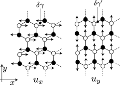
Figure 3: The displacement vectors, $u_{x}$ and $u_{y}$, of the $\Gamma$ point optical phonon modes. $\delta\gamma$ ($\delta\gamma^{\prime}$) represents a change of the nearest-neighbor hopping integral caused by the vibration.

We define $G_{x}$ and $G_{y}$ as follows,

$$\begin{split}\frac{G_{x}}{\delta\gamma}&=\sum_{J=1}^{N}(\phi^{J})^{\dagger}\left[T\sigma_{z}\phi^{J+1}+\sigma_{z}T^{-1}\phi^{J-1}\right]+{\rm c.c.},\\ \frac{G_{y}}{\delta\gamma^{\prime}}&=\sum_{J=1}^{N}(\phi^{J})^{\dagger}\left[\frac{1}{2}\left\{T\phi^{J+1}+T^{-1}\phi^{J-1}\right\}-\sigma_{x}\phi^{J}\right]+{\rm c.c.}\end{split}$$ (32)

It is straightforward to show that $G_{x}$ and $G_{y}$ are the expectation values of the perturbations caused by the lattice displacements $u_{x}$ and $u_{y}$, respectively. Here, $\delta\gamma$ and $\delta\gamma^{\prime}$ are the changes of the hopping integral for the C-C bonds denoted in Fig. 3, produced by the lattice displacements $u_{x}$ and $u_{y}$, respectively. By putting $\phi^{J}_{s}$ of eq. (24) into $\phi^{J}$ of eq. (32), we obtain

$$\begin{split}&G_{x}=0,\\ &\frac{G_{y}}{\delta\gamma^{\prime}}=-3\langle\sigma_{x}\rangle-\epsilon,\end{split}$$ (33)

where $\langle\sigma_{x}\rangle$ is the expectation value of the Pauli matrix $\sigma_{x}$ defined by

$$\langle\sigma_{x}\rangle\equiv\sum_{J=1}^{N}(\phi^{J}_{s})^{\dagger}\sigma_{x}\phi^{J}_{s}=-s\cos\Theta.$$ (34)

In eq. (33), we have obtained $G_{y}$ by putting the energy eigen equation of eq. (6) with $K=\epsilon\sigma_{0}+\sigma_{x}$ into the right-hand side of $G_{y}$ in eq. (32).

We note that this result of $G_{y}$ derived by using tight-binding model is slightly different from the result of an effective-mass theory. The effective-mass theory gives [7]

$$\frac{G_{y}}{\delta\gamma^{\prime}}=-3\langle\sigma_{x}\rangle.$$ (35)

The difference between the two schemes is $\epsilon$. Since $\epsilon$ is scaled by the hopping integral, $\epsilon$ vanishes in the continuum limit, so that this $\epsilon$ term does not appear in the effective mass theory. Here, we consider two direct consequences of the $\epsilon$ term. First, because the Raman intensity is proportional to $G_{y}^{2}$, the $\epsilon$ term may give rise to a small dependence of the Raman intensity on the laser energy. The dependence about 10%$/$eV is acceptable for the process that satisfies $|\langle\sigma_{x}\rangle|\approx 1$. Second, the strength of $G_{y}$ decreases for the state near the top (bottom) at the conduction (valence) band. Thus, the Raman intensity for, if any, such a high energy state should be suppressed strongly.

The result in eq. (33) means that the $u_{x}$ mode is not Raman active mode near the armchair edge and only the $u_{y}$ mode can be Raman active. This is a phenomenon peculiar to armchair edge [14, 7] because it can be shown that the $G_{x}$ and $G_{y}$ do not vanish in the case of a periodic graphene as

$$\begin{split}&\frac{G_{x}}{\delta\gamma}=s\left(\cos(\theta+\Theta)-\cos(\theta-\Theta+kb)\right),\\ &\frac{G_{y}}{\delta\gamma^{\prime}}=-3\langle\sigma_{x}\rangle-\epsilon.\end{split}$$ (36)

Recent experiments for the G band Raman spectroscopy for graphene edge by Cong et al. [22] and Begliarbekov et al. [23] support this prediction.

4 Discussion and Summary

It is often said that a step edge located on top of a highly oriented pyrolytic graphite (HOPG) can have a regular structure over a large length more than 10 nm. [24] The wave function for such a step edge can also be constructed analytically. The equation for a step armchair edge on top of HOPG is given by replacing the matrix $K$ in eq. (6) with $K-m\sigma_{z}$. Here, $m$ represents the potential difference between the A and B sublattice which is induced by the stack in the Bernal configuration. It is easy to show that the spinor eigenstate of eq. (9) is modified by the presence of $m$ as

$$\phi_{+}=\begin{pmatrix}\frac{1-z+\sqrt{(-1+z)^{2}+4z(\epsilon^{2}-m^{2})}}{2z(\epsilon-m)}\cr 1\end{pmatrix}.$$ (37)

Note that the lowest energy state with $k=0$ ($z=1$) in the conduction band has amplitude only on the A-atoms for the case that $m>0$. It is obvious that by taking the limit $\epsilon\to m$ in eq. (37), the normalized spinor is written as

$$\phi_{+}=\begin{pmatrix}1\cr 0\end{pmatrix},$$ (38)

which is a pseudospin polarized state. The electron-density pattern of this state is shown in Fig. 4, where the density forms the hexagonal pattern. It is important to recognize that the appearance of the hexagonal pattern results from two causes: (1) the asymmetry of the potential energies at the A and B sublattice and (2) the existence of armchair edge. The condition (1) is satisfied in the bulk of HOPG [25] and epitaxial graphene on SiC(0001) [26]. The STM images show a triangular lattice there because the amplitude can be observed only at one of the two sublattice for the case that $m\neq 0$. In addition to (1), near the armchair edge (2), the low energy electron does not have amplitude at the sites $J=3i$ [see Fig. 1(b)] due to $\sin(J\theta)$. As a result, a low bias STM topography observes the hexagonal electron-density pattern near a step armchair edge on top of a HOPG. [27, 11]

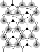
Figure 4: The electron-density pattern of a low-energy state near the armchair step edge located on top of a HOPG. The unit of $(\sqrt{3}a\times\sqrt{3}a)\ 30^{\circ}$ superstructure is shown by the rhombus. This unit cell is the same as that of the Kekulé pattern.

Beside the hexagonal pattern, an electron-density pattern which is referred to as $(\sqrt{3}a\times\sqrt{3}a)\ 30^{\circ}$ or $(\sqrt{3}\times\sqrt{3})R\ 30^{\circ}$ superstructure is frequently observed near defects on graphite, such as metal particles, [28, 29] isolated adsorbed molecules, [30, 31] step edges, [32, 24, 25] and lattice vacancies. [33, 34, 35, 25] This superstructure is denoted by the rhombus in Fig. 4 (see ref. shedd92). The periodicity of the $(\sqrt{3}a\times\sqrt{3}a)\ 30^{\circ}$ superstructure is actually included in the wave function for armchair edge as shown in Fig. 4. Note, however, that the origin of this superstructure observed in the experiments for step edges can not be attributed only to armchair edge since the presence of zigzag edge might play an important role. A simulation by Niimi et al. [27] indicates such a possibility. To fully specify the origin of the $(\sqrt{3}a\times\sqrt{3}a)\ 30^{\circ}$ superstructure, it is desirable to construct analytical wave function for a mixed edge consisting of zigzag and armchair edge parts.

In summary, we have constructed the analytical solution of the tight-binding model for armchair nanoribbon. The wave function is described by the superposition of the incident wave to the armchair edge and the scattered wave, i.e., the formation of standing wave. The scattering process is intervalley scattering, in which the pseudospin is invariant. The difference between armchair nanoribbon and nanotube appears with respect to the number of Dirac singularities in their phase spaces. Since the armchair boundary condition identifies the half of graphene BZ (including the K point) and the other half of the graphene BZ (including the K^′ point), the phase space of armchair nanoribbon is given by the half region of the graphene BZ. As a result, in the phase space of armchair nanoribbon, there is a single Dirac singularity whose wave function is written by the antisymmetric combination of the two states at the K and K^′ points. We have examined the recent STM topography by using the analytic solution. It seems that the STM image obtained by Yang et al. [10] corresponds to a state away from the Dirac singularity. This speculation is consistent with the appearance of a long-range oscillation in their STM image. Moreover, the observed STM image does not allow assuming the existence of a strong boundary potential of order of the hopping integral. A lattice distortion at armchair edge can be taken into account as a shift of the Dirac singularity point along the $\theta$-axis, which is similar to the curvature effect in metallic carbon nanotubes. In addition, the analytical solution allows us to observe easily that $u_{x}$ mode is not Raman active near the armchair edge. The analytical solution simplifies greatly the analysis which was done numerically with the tight-binding model, [14] and is also useful for confirming the result obtained analytically with the effective-mass model [7].

References

- [1] R. Saito, M. Fujita, G. Dresselhaus, and M. S. Dresselhaus: Appl. Phys. Lett. 60 (1992) 2204.
- [2] K. S. Novoselov, D. Jiang, F. Schedin, T. J. Booth, V. V. Khotkevich, S. V. Morozov, and A. K. Geim: Proceedings of the National Academy of Sciences 102 (2005) 10451.
- [3] A. K. Gupta, T. J. Russin, H. R. Gutie ̵̡ rez, and P. C. Eklund: ACS Nano 3 (2009) 45.
- [4] X. Jia, M. Hofmann, V. Meunier, B. G. Sumpter, J. Campos-Delgado, J. M. Romo-Herrera, H. Son, Y.-P. Hsieh, A. Reina, J. Kong, M. Terrones, and M. S. Dresselhaus: Science 323 (2009) 1701.
- [5] K. Sasaki, K. Wakabayashi, and T. Enoki: New J. Phys. 12 (2010) 083023.
- [6] L. G. Cançado, M. A. Pimenta, B. R. A. Neves, M. S. S. Dantas, and A. Jorio: Phys. Rev. Lett. 93 (2004) 247401.
- [7] K. Sasaki, R. Saito, K. Wakabayashi, and T. Enoki: J. Phys. Soc. Jpn. 79 (2010) 044603.
- [8] K. Tanaka, S. Yamashita, H. Yamabe, and T. Yamabe: Synthetic Metals 17 (1987) 143 .
- [9] M. Fujita, K. Wakabayashi, K. Nakada, and K. Kusakabe: J. Phys. Soc. Jpn. 65 (1996) 1920.
- [10] H. Yang, A. J. Mayne, M. Boucherit, G. Comtet, G. Dujardin, and Y. Kuk: Nano Lett. 10 (2010) 943.
- [11] K.-i. Sakai, K. Takai, K.-i. Fukui, T. Nakanishi, and T. Enoki: Phys. Rev. B 81 (2010) 235417.
- [12] S. Compernolle, L. Chibotaru, and A. Ceulemans: J. Chem. Phys. 119 (2003) 2854.
- [13] H. Zheng, Z. F. Wang, T. Luo, Q. W. Shi, and J. Chen: Phys. Rev. B 75 (2007) 165414.
- [14] K. Sasaki, M. Yamamoto, S. Murakami, R. Saito, M. Dresselhaus, K. Takai, T. Mori, T. Enoki, and K. Wakabayashi: Phys. Rev. B 80 (2009) 155450.
- [15] H. Y. Zhu, D. J. Klein, T. G. Schmalz, A. Rubio, and N. H. March: J. Phys. Chem. Solids 59 (1998) 417 .
- [16] T. Sato, M. Tanaka, and T. Yamabe: Synthetic Metals 103 (1999) 2525 .
- [17] K. Wakabayashi, M. Fujita, H. Ajiki, and M. Sigrist: Phys. Rev. B 59 (1999) 8271.
- [18] D. A. Areshkin, D. Gunlycke, and C. T. White: Nano Lett. 7 (2007) 204.
- [19] G. Treboux, P. Lapstun, and K. Silverbrook: Chem. Phys. Lett. 302 (1999) 60 .
- [20] M. Fujita, M. Igami, and K. Nakada: J. Phys. Soc. Jpn. 66 (1997) 1864.
- [21] K. Sasaki, Y. Shimomura, Y. Takane, and K. Wakabayashi: Phys. Rev. Lett. 102 (2009) 146806.
- [22] C. Cong, T. Yu, and H. Wang: ACS Nano 4 (2010) 3175.
- [23] M. Begliarbekov, O. Sul, S. Kalliakos, E.-H. Yang, and S. Strauf: Appl. Phys. Lett. 97 (2010) 031908.
- [24] P. L. Giunta and S. P. Kelty: J. Chem. Phys. 114 (2001) 1807.
- [25] L. Tapasztó, P. Nemes-Incze, Z. Osváth, M. Bein, A. Darabont, and L. Biró: Physica E 40 (2008) 2263.
- [26] G. M. Rutter, J. N. Crain, N. P. Guisinger, T. Li, P. N. First, and J. A. Stroscio: Science 317 (2007) 219.
- [27] Y. Niimi, T. Matsui, H. Kambara, K. Tagami, M. Tsukada, and H. Fukuyama: Phys. Rev. B 73 (2006) 085421.
- [28] G. M. Shedd and P. E. Russell: Surf. Sci. 266 (1992) 259.
- [29] J. Valenzuela-Benavides and L. M. la Garza: Surf. Sci. 330 (1995) 227 .
- [30] H. A. Mizes and J. S. Foster: Science 244 (1989) 559.
- [31] K. F. Kelly, E. T. Mickelson, R. H. Hauge, J. L. Margrave, and N. J. Halas: Proceedings of the National Academy of Sciences of the United States of America 97 (2000) 10318.
- [32] T. R. Albrecht, H. A. Mizes, J. Nogami, S. il Park, and C. F. Quate: Appl. Phys. Lett. 52 (1988) 362.
- [33] R. Coratger, A. Claverie, A. Chahboun, V. Landry, F. Ajustron, and J. Beauvillain: Surf. Sci. 262 (1992) 208 .
- [34] J. Yan, Z. Li, C. Bai, W. S. Yang, Y. Wang, W. Zhao, Y. Kang, F. C. Yu, P. Zhai, and X. Tang: J. Appl. Phys. 75 (1994) 1390.
- [35] P. Ruffieux, M. Melle-Franco, O. Gröning, M. Bielmann, F. Zerbetto, and P. Gröning: Phys. Rev. B 71 (2005) 153403.