Game Theoretical Power Control for Open-Loop Overlaid Network MIMO Systems with Partial Cooperation

Abstract

Network MIMO is considered to be a key solution for the next generation wireless systems in breaking the interference bottleneck in cellular systems. In the MIMO systems, open-loop transmission scheme is used to support mobile stations (MSs) with high mobilities because the base stations (BSs) do not need to track the fast varying channel fading. In this paper, we consider an open-loop network MIMO system with $K$ BSs serving K private MSs and $M^{c}$ common MS based on a novel partial cooperation overlaying scheme. Exploiting the heterogeneous path gains between the private MSs and the common MSs, each of the $K$ BSs serves a private MS non-cooperatively and the $K$ BSs also serve the $M^{c}$ common MSs cooperatively. The proposed scheme does not require closed loop instantaneous channel state information feedback, which is highly desirable for high mobility users. Furthermore, we formulate the long-term distributive power allocation problem between the private MSs and the common MSs at each of the $K$ BSs using a partial cooperative game. We show that the long-term power allocation game has a unique Nash Equilibrium (NE) but standard best response update may not always converge to the NE. As a result, we propose a low-complexity distributive long-term power allocation algorithm which only relies on the local long-term channel statistics and has provable convergence property. Through numerical simulations, we show that the proposed open-loop SDMA scheme with long-term distributive power allocation can achieve significant performance advantages over the other reference baseline schemes.

I Introduction

Inter-cell interference (ICI) has been widely considered as a critical performance bottleneck for wireless communications in the cellular networks [1, 2]. For instance, mobile stations (MSs) at the cell edge (within the coverage of multiple base stations (BSs)) are usually interference limited. To alleviate the interference issues, traditional cellular systems employ frequency reuse so as to control the interference at the expense of poor spectral efficiency [3]. On the other hand, network MIMO communications [4, 5] are considered to be a key solution for the next generation wireless systems in breaking the interference bottleneck in cellular systems. The idea of network MIMO communications is to utilize cooperation among multiple BSs for joint signal processing in the uplink/downlink directions. Through cooperation, the undesired ICI can be transformed into useful signals via the collaborative transmission among adjacent BSs [6, 7].

One key challenge in network MIMO systems is on how to spatially multiplex multiple MSs effectively and efficiently. Traditionally, linear precoding (such as Tx-MMSE [8] or zero-forcing [9]) could be used to spatially multiplex MSs but closed loop knowledge of instantaneous channel state information (CSI) is required at the BS and this refers to closed-loop spatial division multiplexing access (SDMA)[10, 11]. However, the closed-loop SDMA schemes only work for low mobility MSs where the channel conditions remain quasi-static within the transmission duration. For the high mobility MSs, it is very difficult to keep track of the channel state information (CSI) at the BSs and hence, the above closed-loop schemes cannot be applied for high mobility MSs.

Open-loop transmission scheme has been widely considered in the existing literature for high mobility users. By open-loop schemes, we mean that instantaneous CSI knowledge is not required at the BS. For example, in [12, 13], the authors proposed an open-loop transmission scheme, namely the space-time block code (STBC) for point-to-point scenarios. In [14], double-STTD which is able to serve two users simultaneously has been proposed for 4 transmit antenna and 2 receive antenna MIMO link to fully exploit the spatial diversity and spatial multiplexing gains. All the above open-loop schemes only work in a single cell scenario and there are several important technical challenges to extend to multi-cell systems. They are elaborated below.

• Heterogeneous Path Gain and Shadowing Effect In the network MIMO systems, the path gains of different MSs are quite different. The heterogeneous path gain effect for different types of MSs leads to significant power efficiency loss and hence the conventional open-loop transmission schemes (which have ignored the heterogeneous path gain and shadowing effects) cannot be directly applied in the network MIMO.

• Dynamic and Heterogeneous MIMO Configurations In the network MIMO systems, the number of cooperating BSs is changing dynamically and hence, we are not able to use existing STBC structures in such dynamic MIMO configurations (with time varying number of transmit antennas).

In this paper, we consider a network MIMO system with multiple BSs and multiple high mobility MSs. We propose a novel open-loop scheme to serve $K$ private MSs and $M^{c}$ common MSs simultaneously based on novel partial cooperative overlaying. Specifically, each BS serves a private MS non-cooperatively. By exploiting the path gain difference between the common MSs and the private MS, the $K$ BSs also serve the $M^{c}$ common MSs cooperatively at the same spectrum as the private MSs. The proposed scheme does not require knowledge of instantaneous CSI at the BS and supports dynamic and flexible network MIMO configurations. Furthermore, to adjust the long-term power allocation between the common MSs and the private MS at each of the $K$ BSs, we formulate the long-term distributive power control problem using a partial cooperative game formulation. We show that the long-term power control game has a unique Nash Equilibrium (NE) but the conventional best response update algorithm cannot always converge to the NE. As a result, we propose a low-complexity distributive long-term power allocation algorithm which only relies on the local channel statistics and has provable convergence property. Through numerical simulations, we show that the proposed open-loop overlaying scheme with a distributive long-term power allocation algorithm can achieve significant performance advantages over the traditional schemes and the distributive algorithm has negligible performance loss compared with the centralized power allocation scheme.

I-A Notations

We adopt the following notation conventions. Boldface upper case letters denote matrices, boldface lower case letters denote column vectors, and lightface italics denote scalers. $\mathbb{C}^{n\times m}$ denotes the set of ${n\times m}$ matrices with complex-valued entries and the superscript $(.)^{H}$ denotes Hermitian transpose operation. The matrix $\mathbf{I}_{n}$ denotes the $n\times n$ identity matrix. Expressions $P_{r}(x)$ denotes the probability density function (p.d.f.) of the random variable $x$. The expectation with respect to $x$ is written as $\mathbb{E}_{x}[\cdot]$ or simply as $\mathbb{E}[\cdot]$.

II System Model

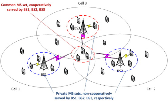
Figure 1: An example of network configuration containing three cells. MSs in the solidline red circle represent the common MS set which is served cooperatively by all the BSs within coverage. MSs in the solidline blue circle represent the private MS sets which are served non-cooperatively in the coverage of BS1, BS2, and BS3, respectively.

Consider a cellular network where there are $K$ base stations (BSs) and $M$ high mobility mobile stations (MSs) as shown in Figure 1. We assume each BS is equipped with $N_{t}$ transmit antennas and each MS is equipped with $N_{r}$ receive antennas.

Denote $T$ to be the transmission time intervals and $\mathbf{S}_{k}\in\mathbb{C}^{N_{t}\times T}$ to be the transmitted signals from the $k$-th BS. The received signals of $m$-th MS, denoted by $\mathbf{Y}_{m}\in\mathbb{C}^{N_{r}\times T}$, can thus be modeled as follows,

$$\mathbf{Y}_{m}=\sum_{k=1}^{K}\sqrt{P_{k}L_{mk}}\mathbf{H}_{mk}\mathbf{S}_{k}+\mathbf{Z}_{m},\ \forall m=1,2,\ldots,M$$ (1)

where $\mathbf{H}_{mk}\in\mathbb{C}^{N_{r}\times N_{t}}$ is the normalized complex fading coefficients from the $k$-th BS to the $m$-th MS, $\mathbf{Z}_{m}\in\mathbb{C}^{N_{r}\times T}$ is the additive white complex Gaussian noise (AWGN) with zero mean and unit variances, $P_{k}$ denotes the transmit power of the $k$-th BS and $L_{mk}$ denotes the long-term path gain and shadowing from the $k$-th BS to the $m$-th MS.

The following assumptions are made through the rest of the paper. Firstly, all the receivers in the system have perfect CSI of each corresponding link, i.e. the $l$-th MS has the perfect CSI knowledge from the $k$-th BS. Secondly, we assume all the BSs have no instantaneous CSI knowledge $\{\mathbf{H}_{mk},m=1,2,\ldots,M,k=1,2,\ldots,K\}$. Thirdly, all the entries of the channel coefficient matrix $\{\mathbf{H}_{mk},m=1,2,\ldots,M,k=1,2,\ldots,K\}$ are independent and identical distributed (i.i.d.) complex Gaussian random variables with zero mean and unit variance. Moreover, we consider block fading channels where the aggregate CSI $\mathbf{H}=\{\mathbf{H}_{mk},m=1,2,\ldots,M,k=1,2,\ldots,K\}$ remains quasi-static within a fading block (i.e. the transmission time interval $T$) but varies between different fading blocks.

III Problem Formulation

In this section we shall first introduce a user scheduling algorithm, which classifies the high mobility MSs into $K$ private MS sets (one for each BS) and a common MS set (shared by all the BS). Based on the user scheduling algorithm, we propose a novel open loop scheme to overlay the MSs in the common set and the private sets simultaneously using partial cooperation. We shall then discuss the problem formulation of the long-term power allocation control in what follows.

III-A Long-term User Scheduling Algorithm

We first define the private MS set and the common MS set below.

Definition 1 (Common/Private MS Sets)

• $k$-th Private MS Set: The $k$-th private MS set $\mathcal{U}_{k}^{p}$ consists of one MS (the $m$-th MS) in which the long-term path gain and shadowing configuration $\{L_{m1},L_{m2},\ldots,L_{mK}\}$ satisfies the following criteria: $L_{mk}-L_{mj}>\xi_{k}^{p},\forall j\neq k$, where $\xi_{k}^{p}$ is the $k$-th private MS set threshold.

• Common MS Set: The common MS set $\mathcal{U}^{c}$ consists of at most $M^{c}$ MSs such that $|L_{mk}-\frac{1}{K}\sum_{j=1}^{K}L_{mj}|\leq\xi^{c},\forall k=1,2,\ldots,K$ for all $m\in\mathbf{U}^{c}$, where $\xi^{c}$ is the common MS set threshold.

Remark 1

To ensure $\mathcal{U}^{c}\bigcap\mathcal{U}^{p}_{k}=\varnothing$ for all $k=1,\ldots,K$, the thresholds need to satisfy $\xi_{k}^{p}\geq\frac{K-1}{K}\xi^{c}$ for all $k=1,\ldots,K$. As such, the private MS sets consist of MSs closer to the home cell whereas the common MS set consists of the MSs closer to the ”coverage overlap areas” between the BSs.

Remark 2

On the other hand, a MS may belong to neither of the above two set. In that case, the MS is not selected to be the ”common MS” or the ”private MS” and does not participate in the ”open loop overlaying scheme”. This MS may be served in the normal way (e.g. assigned another sub-band). Since the MS are moving around, this particular MS may be able to be selected as the ”common MS” or ”private MS” in some future time.

Algorithm 1 illustrates a low complexity user scheduling algorithm to construct $\mathcal{U}^{p}_{k},k=1,\ldots,K$ and $\mathcal{U}^{c}$ based on the local long-term path gain and shadowing at each of the MSs.

Algorithm 1 Long-term User Scheduling Algorithm

• Step 1: MS Broadcast:

  At the $m$-th ($m=1,2,\dots,M$) MS side, the $m$-th MS measures path gains $L_{mk},k=1,\ldots,K$(in dB) from all the $K$ BSs. According to Definition 1, if there exists $L_{mk}$ such that $L_{mk}-L_{mj}>\xi_{k}^{p},\forall j\neq k$, then the $m$-th MS labels itself as a potential member of the $k$th private MS set; if $\forall k=1,2,\ldots,K$, $|L_{mj}-\frac{1}{K}\sum_{j=1}^{K}L_{mj}|\leq\xi^{c}$, then the $m$-th MS labels itself as a potential member of the common MS set. Those MS being potential members of the private set or the common set will then broadcasts its (label,BS$\_$ID) to all the $K$ BSs.

• Step 2: Formation of the Private MS Set:

  Denote $\mathcal{U}_{k}^{p},k=1,2,\dots,K$ to be the $k$-th private MS set. The k-th BS picks one MS with label = ”private” and BS$\_$ID = $k$ to be the member of the private MS set $\mathcal{U}_{k}^{p},k=1,2,\dots,K$ randomly.

• Step 3: Formation of the common MS Set:

  Denote $\mathcal{U}^{c}_{k}$ to be the potential common MS set at the $k$-th BS. Assign the $m$-th MS to $\mathcal{U}^{c}_{k}$ at the $k$-th BS if the label from the $m$-th MS is ”COMMON”. Each BS then submits $\mathcal{U}_{k}^{c}$ to the base station controller (BSC). At the BSC, the common MS set $\mathcal{U}^{c}$ is chosen as an intersection of $\mathcal{U}_{k}^{c},k=1,2,\dots,K$, i.e. $\bigcap_{k=1}^{K}\mathcal{U}_{k}^{c}$. If the number of members in the intersection exceeds $M^{c}$, then $M^{c}$ users will be selected randomly.

III-B Signal Model for the Private/Common MS

Given the user sets $\mathcal{U}^{p}_{k},k=1,\ldots,K$ and $\mathcal{U}^{c}$, the received signal of the $m$-th MS in the private and common MS sets, denoted by $\mathbf{Y}_{m}$ , is given by:

$$\mathbf{Y}_{m}=\left\{\begin{array}[]{ll}\sum_{k=1}^{K}\sqrt{P_{k}L_{mk}}\mathbf{H}_{mk}\mathbf{S}_{k}+\mathbf{Z}_{m},&\qquad m\in\mathcal{U}^{c}\\ \sqrt{P_{k}L_{mk}}\mathbf{H}_{mk}\mathbf{S}_{k}+\mathbf{Z}_{m},&\qquad m\in\mathcal{U}^{p}_{k}\end{array}\right.$$ (4)

Remark 3

At the private MS, inter-cell interference doesn’t appear in the received signal model because the inter-cell interference at the private MS is very weak and negligible. For instance, if $\xi_{k}^{p}=20$dB, $k=1,2,\ldots,K$, the inter-cell interference would be 100 times less than the useful signal.

III-C Open-Loop Overlaying Transmission/Dection Scheme

III-C1 Open-Loop Overlaying Transmission Scheme

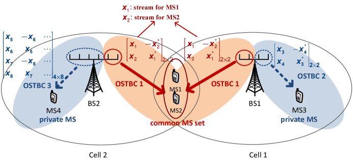
Figure 2: An illustrative diagram of the transmit structure at each BS. For example, the BS1 and BS2 are serving the common set (MS1 and MS2) cooperatively with the same OSTBC (in which stream x1 is for MS1 and stream x2 is for MS2) and serving the private MS3 and MS4 using two different OSTBC structures respectively.

Consider the information streams for the $M^{c}$ MSs in the common MS set (denoted by $\mathbf{X}_{j},j\in\mathcal{U}^{c}$) and the information streams for the $l$-th MS (in the $k$-th private MS set) (denoted by $\mathbf{X}_{l},l\in\mathcal{U}^{p}_{k}$) are transmitted over the $N_{t}$ antennas at the $k$-th BS. To exploit the possible diversity provided by the transmit antenna arrays, orthogonal space-time block code (OSTBC) [15, 12] scheme is applied for transmission, which spans over the entire transmitting antennas. The information streams ($\mathbf{X}_{l},l\in\mathcal{U}^{c}$) for the $M^{c}$ common MSs are jointly encoded as the OSTBC $\mathbf{S}^{c}$ and the information streams for the MS in the $k$-th private MS set is encoded as the OSTBC $\mathbf{S}^{p}_{k}$ as shown in Fig. 2. Without loss of generality, we assume at the $k$-th BS, the two OSTBCs $\mathbf{S}^{p}_{k}$ and $\mathbf{S}^{c}$ are delivered through $N_{t}^{p}$ and $N_{t}^{c}$ transmit antennas respectively with $N_{t}^{p}+N_{t}^{c}=N_{t}$. So the transmitted symbols at the $k$-th BS are given by $\mathbf{S}_{k}=\left[(\mathbf{S}^{p}_{k})^{T}\ (\mathbf{S}^{c})^{T}\right]^{T}$.

For illustration purpose, let us consider a specific case with $M^{c}=2$. Assume $N_{t}=4$ with $N_{t}^{p}=N_{t}^{c}=2$. At each BS, the two information streams for two MSs in the common MS set respectively are jointly OSTBC encoded into one Alamouti’s structure [15] and the information streams for the $k$-th private MS set are encoded as the other Alamouti structure. The whole transmit structure is also known as double space-time transmit diversity (D-STTD) [14]. The transmitted structure at the $k$-th BS is given by:

$$\mathbf{S}_{k}=\sqrt{\frac{\theta_{k}^{p}}{N_{t}^{p}}}\left[\begin{array}[]{cc}s_{k,1}^{p}&-s_{k,2}^{p,*}\\ s_{k,2}^{p}&s_{k,1}^{p,*}\\ 0&0\\ 0&0\end{array}\right]+\sqrt{\frac{\theta_{k}^{c}}{N_{t}^{c}}}\left[\begin{array}[]{cc}0&0\\ 0&0\\ s_{1}^{c}&-s_{2}^{c,*}\\ s_{2}^{c}&s_{1}^{c,*}\end{array}\right]$$ (5)

where $\mathbf{S}^{p}_{k}=\left[\begin{array}[]{cc}s_{k,1}^{p}&-s_{k,2}^{p,*}\\ s_{k,2}^{p}&s_{k,1}^{p,*}\end{array}\right]$ and $\mathbf{S}^{c}=\left[\begin{array}[]{cc}s_{1}^{c}&-s_{2}^{c,*}\\ s_{2}^{c}&s_{1}^{c,*}\end{array}\right]$, $\theta_{k}^{p}$ is the power allocation ratio for the private MS set in the coverage of the $k$-th BS and $\theta_{k}^{c}$ is the power allocation ratio for the common MS set at the $k$-th BS. $\theta_{k}^{p}$ and $\theta_{k}^{c}$ satisfy the relation $\theta_{k}^{p}+\theta_{k}^{c}=1$.

The proposed open-loop oveylaying scheme has the following advantages.

• Exploiting the Heterogeneous Path Gain: As we have mentioned before, the heterogeneous path gain effect for different types of MSs leads to significant power efficiency loss and hence the conventional open-loop transmission schemes cannot be directly applied in the network MIMO system. With the proposed open-loop overlaying scheme, the common MS and the private MS can be simultaneously served. Due to the long-term power splitting ratio $\theta_{k}^{c}$ and $\theta_{k}^{p}$, we can efficiently control the ICI generated at the common MS side under different path gain configurations through the carefully designed long-term power allocation schemes to enhance the power efficiency for the private MS.

• Exploiting Flexible MIMO Configurations: In the proposed open-loop overlaying scheme, we could accommodate dynamic and heterogenous MIMO configurations in the systems. This can be illustrated through the following simple example. Consider three cooperative BSs with heterogeneous MIMO configurations, e.g. BS1 is equipped with $4$ antennas, BS2 is equipped with $6$ antennas and BS3 is equipped with $3$ antennas. Due to mobility of users, assume BS1 and BS2 cooperatively serve one common MS in the first time slot and BS2 and BS3 cooperatively serve the common MS in the second time slot. In the traditional open-loop overlaying scheme, the STBC design has to accommodate BS3 with three transmit antennas for both time slots. However, for the proposed open-loop overlaying scheme as illustrated in Fig. 2, BS1 and BS2 can use the remaining 2 and 4 transmit antennas for the private MSs . In the second time slot, BS2 and BS3 can perform the similar operations to serve the private MSs with the remaining transmit antennas. As a result, the proposed open-loop overlaying scheme offers flexibility with respect to dynamic and heterogeneous MIMO configurations in the systems.

III-C2 Open-loop Overlaying Detection Scheme

Applying the above transmission scheme, the received signals at the common MS can be modeled as:

$$\mathbf{Y}_{m} = \sum_{k=1}^{K}\sqrt{P_{k}L_{mk}}\big{[}\mathbf{H}_{mk,1}\quad\mathbf{H}_{mk,2}\big{]}\left[\begin{array}[]{c}\sqrt{\frac{\theta_{k}^{p}}{N_{t}^{p}}}\mathbf{S}^{p}_{k}\\ \sqrt{\frac{\theta_{k}^{c}}{N_{t}^{c}}}\mathbf{S}^{c}\end{array}\right]+\mathbf{Z}_{m}$$ (8)

$$= \underbrace{\sum_{k=1}^{K}\sqrt{\frac{P_{k}L_{mk}\theta_{k}^{c}}{N_{t}^{c}}}\mathbf{H}_{mk,2}\mathbf{S}^{c}}_{\textrm{Signal Part}}+\underbrace{\sum_{k=1}^{K}\sqrt{\frac{P_{k}L_{mk}\theta_{k}^{p}}{N_{t}^{p}}}\mathbf{H}_{mk,1}\mathbf{S}_{k}^{p}+\mathbf{Z}_{m}}_{\textrm{Interference + Noise Part}},\qquad\forall m\in\mathcal{U}^{c}$$ (9)

Similarly, the received signals at the private MS can be modeled as:

$$\mathbf{Y}_{m} = \sqrt{P_{k}L_{mk}}\big{[}\mathbf{H}_{mk,1}\quad\mathbf{H}_{mk,2}\big{]}\left[\begin{array}[]{c}\sqrt{\frac{\theta_{k}^{p}}{N_{t}^{p}}}\mathbf{S}^{p}_{k}\\ \sqrt{\frac{\theta_{k}^{c}}{N_{t}^{c}}}\mathbf{S}^{c}\end{array}\right]+\mathbf{Z}_{m}$$ (12)

$$= \underbrace{\sqrt{\frac{P_{k}L_{mk}\theta_{k}^{p}}{N_{t}^{p}}}\mathbf{H}_{mk,1}\mathbf{S}_{k}^{p}}_{\textrm{Signal Part}}+\underbrace{\sqrt{\frac{P_{k}L_{mk}\theta_{k}^{c}}{N_{t}^{c}}}\mathbf{H}_{mk,2}\mathbf{S}^{c}+\mathbf{Z}_{m}}_{\textrm{Interference + Noise Part}},\qquad\forall m\in\mathcal{U}_{k}^{p}$$ (13)

where $\mathbf{H}_{mk,1}\in\mathbb{C}^{N_{r}\times N_{t}^{p}}$; $\mathbf{H}_{mk,2}\in\mathbb{C}^{N_{r}\times N_{t}^{c}}$. $\mathbf{S}_{k}^{p}$ and $\mathbf{S}^{c}$ denote the OSTBC encoded transmitted matrices for the private MS in the coverage of $k$-th BS and the common MS set with entries $\pm s_{k,1}^{p}$, $\pm s_{k,1}^{p,*}$, $\ldots$, $\pm s_{k,R^{p}_{k}T}^{p}$, $\pm s_{k,R^{p}_{k}T}^{p,*}$ and $\pm s_{k,1}^{c}$, $\pm s_{k,1}^{c,*}$, $\ldots$, $\pm s_{k,R^{c}T}^{c},\pm s_{k,R^{c}T}^{c,*}$ respectively. $R_{k}^{p}$ is the encoding rate for the OSTBC $\mathbf{S}^{p}_{k}$ and $R^{c}$ is the encoding rates for the OSTBC $\mathbf{S}^{c}$.

At the common MS side, the received signals are radio-frequency(RF)-combined to exploit the macro-diversity. Based on (8), each MS in the common MS set shall detect the whole OSTBC $\mathbf{S}^{c}$ by treating the interfering streams $\mathbf{S}^{p}_{k},k=1,2,\ldots,K$ as noise and then take the desired stream from the decoded OSTBC $\mathbf{S}^{c}$. At the private MS side, the received signal in (12) corresponds to a ”strong interference” scenario and hence, the MS in the $k$-th private MS set shall first detect the interfering streams $\mathbf{S}^{c}$ and then perform successive interference cancelation (SIC) to detect its own information streams $\mathbf{S}_{k}^{p}$.

Using the OSTBC transmission structure and the above detection schemes, the throughput expressions of the common MS and private MSs are summarized in the following lemma.

Lemma 1 (Achievable Throughput)

Using the open-loop overlaying transmission and detection scheme described above, the achievable throughput $\mathcal{C}_{m}$ of the MSs in the common and private MS sets is given by:

$$\mathcal{C}_{m}\approx\overline{\mathcal{C}}_{m}=\left\{\begin{array}[]{l}\begin{array}[]{r}\frac{D_{m}}{D}\min_{j\in\mathcal{U}^{c},l\in\mathcal{U}^{p}_{k},k=1,\ldots,K}\{\overline{\mathcal{C}}_{j}^{c},\overline{\mathcal{C}}^{p}_{l}\},\\ m\in\mathcal{U}^{c}\end{array}\\ \begin{array}[]{r}\log\big{(}1+P_{k}L_{mk}\theta_{k}^{p}R_{k}^{p}\big{)},\\ m\in\mathcal{U}^{p}_{k}\ (k=1,\ldots,K)\end{array}\end{array}\right.$$ (20)

where $\overline{\mathcal{C}}_{j}^{c}=\log\big{(}1+\frac{\sum_{k=1}^{K}P_{k}L_{jk}\theta_{k}^{c}R^{c}}{1+\sum_{k=1}^{K}P_{k}L_{jk}\theta_{k}^{p}R_{k}^{p}}\big{)},j\in\mathcal{U}^{c}$ and $\overline{\mathcal{C}}^{p}_{l}=\log\big{(}1+\frac{P_{k}L_{lk}\theta_{k}^{c}R^{c}}{1+P_{k}L_{lk}\theta_{k}^{p}R_{k}^{p}}\big{)}$ for $l\in\mathcal{U}^{p}_{k}$. $D$ is the total number of streams of OSTBC $\mathbf{S}^{c}$, $D_{m}$ is the number of streams for the $m$-th MS (in the common MS set); $R_{k}^{p}$ and $R^{c}$ are the encoding rate for the OSTBC $\mathbf{S}^{p}_{k}$ and $\mathbf{S}^{c}$ respectively.

Proof:

Please refer to Appendix A for the proof. ∎

Remark 4

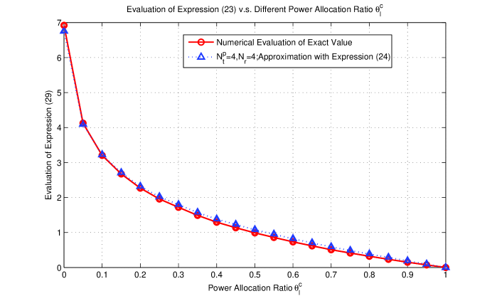
Figure 7: Illustration of the quality of approximation in (41) and (42).

The approximation in (20) is quite tight over a wide range of SNR as illustrated by Figure 7. The physical meaning of $\overline{\mathcal{C}}_{j}^{c},j\in\mathcal{U}^{c}$ is the maximum decodable rate for OSTBC $\mathbf{S}^{c}$ at the $j$-th MS (in the common MS set) by treating the streams ($\mathbf{S}^{p}_{k},k=1,\ldots,K$) for the private MSs as noise and $\overline{\mathcal{C}}^{p}_{l},l\in\mathcal{U}^{p}_{k}$ is the maximum decodable rate at which the $l$th MS (in the $k$-th private MS set) can successfully decode the OSTBC $\mathbf{S}^{c}$ by treating the streams ($\mathbf{S}^{p}_{k}$) for its own as noise. Hence our detection scheme can always work when the transmission rate is given in (20).

III-D Long-term Power Allocation Problem Formulation

It is very important to adjust the long-term power allocation ratio $\{\theta_{k}^{p},\theta_{k}^{c}\}$ to fully exploit the heterogenous path gain and shadowing effect over the network MIMO configuration. In this paper, we consider choosing $\{\theta_{k}^{p},\theta_{k}^{c}\}$ to maximize the minimum weighted throughput (with approximation) which is defined as follows.

Definition 2 (Minimum Weighted Throughput)

Define $\{w_{m},m=1,\ldots,M\}$ to be the positive static weight, which is determined by the Quality-of-Service (QoS) requirement or priority of the $m$-th MS. The minimum weighted throughput of all the MSs (using the approximation in Lemma 1) throughput $\mathfrak{C}$ is given by:

$$\mathfrak{C}\big{(}\{\theta_{k}^{p},\theta_{k}^{c}\}\big{)}=\min_{m\in(\cup_{k=1}^{K}\mathcal{U}^{p}_{k})\cup\mathcal{U}^{c}}\{w_{m}\overline{\mathcal{C}}_{m}\}$$ (21)

where $\overline{\mathcal{C}}_{m}$ is given in (20).

Hence, the optimal long-term power allocation problem can be found by solving the following optimization problem.

$$\big{(}\{\theta_{k}^{p,\star},\theta_{k}^{c,\star}\}\big{)}=\arg\max_{\{\theta_{k}^{p},\theta_{k}^{c}\}} \mathfrak{C}\big{(}\{\theta_{k}^{p},\theta_{k}^{c}\}\big{)}$$

subject to $$\theta_{k}^{p}+\theta_{k}^{c}=1,$$ (22)

$$\theta_{k}^{p},\theta_{k}^{c}\geq 0,$$

$$\forall k\in\{1,\ldots,K\}$$

In general, the above optimization problem (III-D) is non-trivial because of the following reasons. The approximate throughput expression $\overline{\mathcal{C}}_{m}$ involves complicated operations of the power splitting ratio $\{\theta_{k}^{p},\theta_{k}^{c}\}$ which is a composition of logarithm and nonlinear SINR expression. Hence, the objective function is in general non-convex and the standard low complexity algorithms cannot be directly applied. Moreover, as shown in the current literature, this type of problems belongs to the minimum throughput maximization problem for the multi-cell architecture and does not exist a trivial global optimal solution in general [17].

IV Distributive Long-term Power Allocation Algorithms

In this section, our target is to propose a distributed long-term power allocation algorithm based on solving the optimization given by (III-D) in a distributed manner. We formulate the long-term distributive power allocation problem using a partial cooperative game. We show that the long-term power allocation game has a unique Nash Equilibrium (NE). Furthermore, we propose a low-complexity distributive long-term power allocation algorithm which only relies on the local long-term channel statistics and has provable convergence to the NE.

IV-1 Partial Cooperative Game Formulation

We formulate the long-term power allocation design within the framework of game theory as a partial-cooperative game, in which the players are the BSs in the wireless network and the payoff functions are the minimum weighted throughput of MSs in the coverage of each BS. The $k$-th player (BS) competes against the others by choosing his power allocation ratio $\theta^{c}_{k}$ given other players’ power allocation ratio to maximize the minimum weighted throughput $\mathfrak{C}_{k}(\theta^{c}_{k},\bm{\theta^{c}_{-k}})$, which is given by

$$\mathfrak{C}_{k}(\theta^{c}_{k},\bm{\theta}_{-k}^{c})=\min\Big{\{}f_{k}^{1}(\theta_{k}^{c},\bm{\theta}_{-k}^{c}),f_{k}^{2}(\theta_{k}^{c},\bm{\theta}_{-k}^{c})\Big{\}}$$ (23)

where

$$f_{k}^{1}(\theta_{k}^{c},\bm{\theta}_{-k}^{c}) = \min\Big{\{}\min_{j\in\mathcal{U}^{c}}\{w_{j}\frac{D_{j}}{D}\overline{\mathcal{C}}^{c}_{j}\},\min_{j\in\mathcal{U}^{c}}\{w_{j}\frac{D_{j}}{D}\overline{\mathcal{C}}^{p}_{l},l\in\mathcal{U}^{p}_{k}\}\Big{\}}$$ (24)

$$= \min\Big{\{}\underbrace{\min_{j\in\mathcal{U}^{c}}\{w_{j}\frac{D_{j}}{D}\overline{\mathcal{C}}^{c}_{j}\}}_{g^{1}(\bm{\theta}^{c})},\underbrace{\min_{j\in\mathcal{U}^{c}}\{w_{j}\frac{D_{j}}{D}\}\overline{\mathcal{C}}^{p}_{l},l\in\mathcal{U}^{p}_{k}}_{g_{k}^{2}({\theta}_{k}^{c})}\Big{\}}$$

is the minimum weighted throughput (with approximation) of all the MSs in the common MS set,

$$f_{k}^{2}(\theta_{k}^{c},\bm{\theta}_{-k}^{c}) = w_{m}\overline{\mathcal{C}}_{m},m\in\mathcal{U}^{p}_{k}$$ (25)

$$= {w_{m}}\log\left(1+P_{k}L_{mk}(1-\theta_{k}^{c})R_{k}^{p}\right),m\in\mathcal{U}^{p}_{k}$$

is the weighted throughput (with approximation) of the MS in the $k$-th private MS set and $\bm{\theta}^{c}_{-k}\triangleq(\theta_{q}^{c})_{q=1,\ q\neq k}^{K}$ is the set of long-term power allocation ratios of all the BSs except the $k$-th one. Hence, the partial-cooperative game is formulated as:

$$(\mathscr{G}):\quad\left.\begin{array}[]{c c}\max_{\theta_{k}^{c}}&\mathfrak{C}_{k}(\theta^{c}_{k},\bm{\theta}^{c}_{-k})\\ \textrm{subject to}&\bm{\theta}_{k}\in\mathscr{D}_{k}\end{array}\right.\quad\forall k\in\mathscr{K},$$ (28)

where $\mathscr{K}\triangleq\{1,\ldots,K\}$ denotes the set of all players, i.e. the BSs, $\mathfrak{C}_{k}(\theta^{c}_{k},\bm{\theta}^{c}_{-k})$ defined in (23) is the payoff functions of the player $k$ and $\mathscr{D}_{k}$ is the admissible strategy set for player $k$, defined as $\mathscr{D}_{k}\triangleq\{\theta\in\mathbb{R}:0\leq\theta\leq 1\}$. The solutions of the above game $\mathscr{G}$ are formally defined as follows.

Definition 3 (Nash Equilibrium)

A (pure) strategy profile of the long-term power allocation $\bm{\theta}^{c,\star}=(\theta_{k}^{c,\star})_{k\in\mathscr{K}}\in\mathscr{D}_{k}\times\ldots\times\mathscr{D}_{K}$ is a NE of the game $\mathscr{G}$ if

$$\mathfrak{C}_{k}(\theta^{c,\star}_{k},\bm{\theta}^{c,\star}_{-k})\geq\mathfrak{C}_{k}(\theta^{c}_{k},\bm{\theta}^{c,\star}_{-k}),\quad\forall\theta_{k}^{c}\in\mathscr{D}_{k},\ \forall k\in\mathscr{K}.$$ (29)

At a NE point, each BS $k$, given the long-term power allocation profile of other BSs $\bm{\theta}_{-k}^{c,\star}$, cannot improve its utility (or payoff) by unilaterally changing his own long-term power allocation strategy $\theta_{k}^{c}$. The absence of NE simply means that the distributed system is inherently unstable. In order to obtain the distributed solution, we shall characterize the properties of NE such as the existence and uniqueness through the following theorem.

Theorem 1 (Existence and Uniqueness of NE)

The strategic partial-cooperative game $\mathscr{G}$ has the following two properties:

1. There exists a NE for the strategic partial-cooperative game $\mathscr{G}$.

2. Moreover, the NE is unique.

Proof:

Please refer to Appendix B for the proof. ∎

From Theorem 1, we can well establish the properties of the strategic partial-cooperative game $\mathscr{G}$, which is shown to have a unique NE, and hence the distributed system is stable. In the following part, we shall develop the corresponding distributive algorithm to achieve the optimal long-term power allocation for each BS in the overlaid network architecture.

IV-2 Algorithm Description

Since the above partial-cooperative game $\mathscr{G}$ has a unique NE point, we shall try to develop the proper algorithm to find the desired point. Traditionally, in a partial-cooperative game, the best-response update algorithm [18] is shown to achieve good performance. However, the convergence property cannot be guaranteed due to the reason that there might be some best response cycles [19]. In our partial-cooperative game, the best response update can be shown to be not converging to the NE in some cases. In what follows, we shall propose a novel algorithm with provable convergence property.

Algorithm 2 Distributive Long-term Power Allocation Algorithm

• Step 1: Initialization:

  Set iteration index $i=1$.

  For each base station $\mathit{l}\in\mathscr{L}$ choose some power the splitting ratio $\eta_{l}^{c,*}\in[0,1)$ and $\eta_{l}^{p,*}=1-\eta_{l}^{c,*}$ such that $g_{l}^{2}\big{(}\eta_{l}^{c,*}\big{)}=f_{l}^{2}\big{(}\eta_{l}^{c,*}\big{)}$. Under this initial power allocation setup $\bm{\eta^{c,*}}=[\eta_{1}^{c,*},\eta_{2}^{c,*},\ldots,\eta_{L}^{c,*}]$, the common MS broadcasts the measured receive SINR $\Gamma_{\min}(1)$ to all the cooperative BSs.

  Each BS solve the equation $w^{c}\log(1+\Gamma_{\min}(1))=w^{p}_{l}\log(1+P_{l}L_{l}^{p}(1-\theta_{l}^{c})R_{l}^{p})$ with respect to $\theta_{l}^{c}$ to get the root $\xi_{l}^{c}(1)$. Each BS adjust its own power allocation ratio such that $\theta_{l}^{c}(1)=\max\{\xi_{l}^{c}(1),\eta_{l}^{c,*}\}$. Under the power allocation vector $\bm{\theta^{c}}(1)=[\theta_{1}^{c}(1),\theta_{2}^{c}(1),\ldots,\theta_{L}^{c}(1)]$, the common MS broadcasts the measured receive SINR $\Gamma_{\max}(1)$ to all the BSs.

• Step 2: Power Allocation Update:

  Update index $i:=i+1$

  We choose $\Gamma(i)=\big{(}\Gamma_{\min}(i-1)+\Gamma_{\max}(i-1)\big{)}/2$, each BS solves the equation $w^{c}\log(1+\Gamma(i))=w^{p}_{l}\log(1+P_{l}L_{l}^{p}(1-\theta_{l}^{c})R_{l}^{p})$ to get the solution $\xi_{l}^{c}(i)$. Each BS adjusts its own power allocation ratio $\theta_{l}^{c}(i)=\max\{\xi_{l}^{c}(i),\eta_{l}^{c,*}\}$.

• Step 3: Signal and Interference Plus Noise Estimation:

  The common MS broadcasts the measured receive SINR $\overline{\Gamma(i)}$ to all the base stations.

• Step 4: Termination:

  If $\Gamma(i)<\overline{\Gamma(i)}$, $\Gamma_{\min}(i)=\Gamma(i)$ and $\Gamma_{\max}(i)=\Gamma_{\max}(i-1)$.

  If $\Gamma(i)>\overline{\Gamma(i)}$, $\Gamma_{\max}(i)=\Gamma(i)$ and $\Gamma_{\min}(i)=\Gamma_{\min}(i-1)$.

  If $\Gamma(i)=\overline{\Gamma(i)}$, terminate; otherwise, go to Step 2.

Theorem 2

The proposed iterative power allocation algorithm in Algorithm 2 converges to the unique NE defined by (29).

Proof:

Please refer to Appendix C for the proof. ∎

Remark 5 (Complexity and Signaling Overhead)

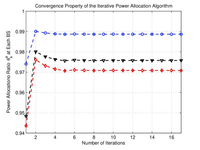
Figure 3: Convergence property of the proposed distributive long-term power allocation algorithm in a cellular network with 3 BSs. Assume the private MS sets and the common MS set have already been determined with our user scheduling algorithm. As a result, 3 BSs non-cooperatively serve 3 private MSs (MS1,MS2 and MS3) respectively and two ($M^{c}=2$) common MS (MS4 and MS5) cooperatively. In the simulation, we choose $P_{1}=P_{2}=P_{3}=30dBm;L_{11}=-118.30dB,L_{12}=-140.14dB,L_{13}=-139.29dB;L_{21}=-145.11dB,L_{22}=-115.56dB,L_{23}=-143.23dB;L_{31}=-147.78dB,L_{32}=-139.65dB,L_{33}=-116.35dB;L_{41}=-135.24dB,L_{42}=-136.08dB,L_{43}=-135.35dB;L_{51}=-135.16dB,L_{52}=-135.91dB,L_{53}=-134.94dB$ and the QoS weighting coefficients are given by $w_{1}=w_{5}=2,w_{2}=w_{3}=w_{4}=1$.

The computation of the long-term power allocation is distributed at each of the $K$ BSs. Furthermore, the iterations are done over a long time scale (instead of short-term CSI time scale) where each common MS shall broadcast its long-term SINR, which is a scalar, in each iteration. As a result, the signaling overhead is very low. Furthermore, as illustrated in Fig. 3, the algorithm has fast convergence and hence, the total iterations required are very limited.

Fig. 3 shows the convergence property of the proposed power allocation algorithm as specified in the figure caption. Through the numerical studies, we found that the proposed long-term power allocation algorithm is shown to have a fast convergence.

V Numerical Examples

This section provides some numerical examples to verify the behavior of our proposed long-term power allocation strategies in a network MIMO configuration with $10$ cells arranged in a hexagonal manner. Each cell has 5km radius and there are 50 type-I MSs (regular MS with weight 1) and 50 type-II MSs (higher priority MSs with weight 2) in the system. These MSs are moving with high speed in the coverage according to a random-walk model[20]. We also assume each BS is equipped with $4$ antennas, namely $N_{t}=4$, and $N_{t}^{c}=N_{t}^{e}=2$. Each MS is equipped with $2$ antennas, namely $N_{r}=2$. The path gain model is given by $\textrm{PG(dB)}=-130.19-37.6\log_{10}(d\textrm{(km)})$ and shadowing standard deviation is $8$dB as specified in the IEEE 802.16m evaluation methodology[21]. For illustration purpose, we compare our proposed long-term power allocation algorithm with the following baseline schemes. Baseline 1: Orthogonal-Division (TDD/FDD) Based Strategy, i.e., the BSs serve the private and common MSs alternatively in different time/frequency slots. Baseline 2: Uniform Power Allocation, i.e., the BSs serve the private and common MSs simultaneously with uniform power allocation. Baseline 3: Centralized Long-term Power Allocation, i.e., the BSs serve the private and common MSs simultaneously using our open-loop SDMA scheme but the long-term power allocation is computed by the brute-force centralized numerical evaluations of problem (III-D).

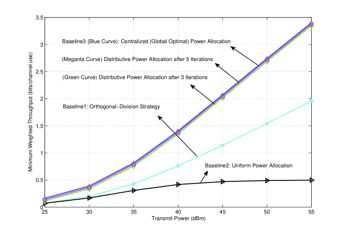
Figure 4: Minimum weighted throughput comparison for different open-loop schemes with respect to the transmit power. Through the numerical examples, the minimum weighted throughput of the proposed distributive long-term power allocation scheme with finite iteration numbers can outperform the conventional orthogonal-division (TDD/FDD) based open-loop scheme (baseline 1) as well as the open-loop overlaying scheme with uniform power allocation (baseline 2) and has negligible performance loss compared to the open-loop overlaying scheme with centralized (global optimal) power allocation (baseline 3). In the simulation, we choose $\xi^{p}_{1}=\ldots=\xi^{p}_{K}=20$dB and $\xi^{c}=5$dB.

Fig. 4 shows the minimum weighted throughput comparison for different open-loop schemes with respect to the BS transmit power. From the numerical examples, we notice that if we apply the open-loop overlaying scheme in a naive manner without careful long-term power allocation, the system performance can even be worse than the traditional orthogonal-division based open-loop scheme (baseline 1 over 2). However, if we utilize the open-loop overlaying scheme with careful long-term power control, the system performance can be greatly improved (baseline 3 and the proposed scheme over baseline 1 and 2). Moreover, the proposed low complexity distributive power allocation algorithm can achieve significant performance advantage over the traditional orthogonal-division (TDD/FDD) schemes (baseline 1) and has negligible performance loss with respect to the centralized scheme (baseline 3). From the simulation results, we observe that the performance of the proposed distributive long-term power allocation algorithm is close-to-optimal (baseline 3). In other words, the NE of the partial cooperative game in (28) is quite ”social optimal”.

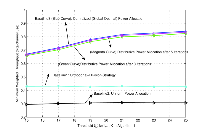
Figure 5: Minimum weighted throughput comparison for different open-loop schemes with respect to the private MS set threshold $\xi^{p}_{k}$ in Algorithm 1. Through the numerical examples, the minimum weighted throughput of the proposed distributive long-term power allocation scheme with finite iteration numbers can outperform the conventional orthogonal-division (TDD/FDD) based open-loop scheme (baseline 1) as well as the open-loop overlaying scheme with uniform power allocation (baseline 2) and has negligible performance loss compared to the open-loop overlaying scheme with centralized (global optimal) power allocation (baseline 3). In the simulation, we keep $\xi^{p}_{1}=\ldots=\xi^{p}_{K}$ and choose $\xi^{c}=5$dB. Transmit Power of all the BSs are 35dBm.

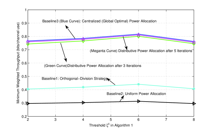
Figure 6: Minimum weighted throughput comparison for different open-loop schemes with respect to the common MS set threshold $\xi^{c}$ in Algorithm 1. Through the numerical examples, the minimum weighted throughput of the proposed distributive long-term power allocation scheme with finite iteration numbers can outperform the conventional orthogonal-division (TDD/FDD) based open-loop scheme (baseline 1) as well as the open-loop overlaying scheme with uniform power allocation (baseline 2) and has negligible performance loss compared to the open-loop overlaying scheme with centralized (global optimal) power allocation (baseline 3). In the simulation, we choose $\xi^{p}_{1}=\ldots=\xi^{p}_{K}=20dB$. Transmit Power of all the BSs are 35dBm.

Fig. 5 and Fig. 6 show the minimum weighted throughput comparison for different open-loop schemes with respect to the private and common MS set thresholds $\xi^{p}_{k}$ and $\xi^{c}$ in Algorithm 1 respectively. We observe the performance gain of the proposed open-loop overlaying scheme over various baselines at various threshold values.

Moreover, the numerical result in Fig. 5 and Fig. 6 again show that the NE of our partial cooperative game in (28) is almost ”social optimal”.

VI Conclusion

In this paper, we proposed an open-loop overlaying scheme to adjust the dynamic and heterogeneous MIMO configurations in the network MIMO systems. To exploit the heterogeneous path gain effect among multiple cells, we propose a distributive low complexity long-term power allocation algorithm with provable convergence property which only relies on local channel statistics. Through numerical studies, we show that the proposed open-loop overlaying scheme with distributive long-term power allocation algorithm can achieve significant performance advantages over the traditional schemes and has negligible performance loss compared with the centralized scheme.

Appendix A Proof of Lemma 1

Denote $\mathcal{C}^{c}$ to be transmission data rate of the OSTBC $\mathbf{S}^{c}$, also denote $\mathcal{C}^{p}_{l},l\in\mathcal{U}^{p}_{k}$ to be the maximum decodable rate at which the $l$-th private MS ($l\in\mathcal{U}^{p}_{k}$) can successfully decode the steams for the common MS set, i.e. OSTBC $\mathbf{S}^{c}$. The expression of $\mathcal{C}{p}_{l}$ is given by:

$$\mathcal{C}^{p}_{l}=\mathbb{E}\big{[}\log(1+\gamma^{p}_{l})\big{]}$$ (30)

where $\gamma_{l}^{p}$ is the instantaneous SINR at the $l$-th MS (in the $k$-th private MS set) when decoding OSTBC $\mathbf{S}^{c}$ by treating OSTBC $\mathbf{S}_{k}^{p}$ as noise and is given by:

$$\gamma_{l}^{p}=\frac{\textrm{Tr}\left\{\left(\sqrt{\frac{P_{k}L_{lk}\theta_{k}^{c}}{N_{t}^{c}}}\mathbf{H}_{lk,2}\mathbf{S}^{c}\right){\left(\sqrt{\frac{P_{k}L_{lk}\theta_{k}^{c}}{N_{t}^{c}}}\mathbf{H}_{lk,2}\mathbf{S}^{c}\right)}^{H}\right\}}{\textrm{Tr}\left\{\left(\sqrt{\frac{P_{k}L_{lk}\theta_{k}^{p}}{N_{t}^{p}}}\mathbf{H}_{lk,1}\mathbf{S}_{k}^{p}+\mathbf{Z}_{l}\right){\left(\sqrt{\frac{P_{k}L_{lk}\theta_{k}^{p}}{N_{t}^{p}}}\mathbf{H}_{lk,1}\mathbf{S}_{k}^{p}+\mathbf{Z}_{l}\right)}^{H}\right\}}\qquad l\in\mathcal{U}^{p}_{k}$$ (31)

where $\textrm{Tr}(\cdot)$ denotes the matrix trace operation. Hence SIC can be performed at the $l$-th MS only when $\mathcal{C}^{c}\leq\mathcal{C}^{p}_{l}$ and the achievable throughput for the $l$-th MS after SIC is given by

$$\mathcal{C}_{l}=\mathbb{E}\big{[}\log(1+\lambda_{l})\big{]}\qquad l\in\mathcal{U}^{p}_{k}$$ (32)

where $\lambda_{l}$ denotes the instantaneous SNR (after the interference cancelation) at $l$-th MS (in the $k$-th private MS set) and is given by:

$$\lambda_{l}=\frac{\textrm{Tr}\big{\{}(\sqrt{\frac{P_{k}L_{lk}\theta_{k}^{p}}{N_{t}^{p}}}\mathbf{H}_{lk,1}\mathbf{S}_{k}^{p})(\sqrt{\frac{P_{k}L_{lk}\theta_{k}^{p}}{N_{t}^{p}}}\mathbf{H}_{lk,1}\mathbf{S}_{k}^{p})^{H}\big{\}}}{\textrm{Tr}\big{\{}\mathbf{Z}_{l}\mathbf{Z}_{l}^{H}\big{\}}},\qquad l\in\mathbf{U}^{p}_{k}$$ (33)

Let $\mathcal{C}_{j}^{c}=\mathbb{E}\big{[}\log(1+\gamma^{c}_{j})\big{]},j\in\mathcal{U}^{c}$ be the maximum decodable rate for the OSTBC $\mathbf{S}^{c}$ at the $j$-th MS (in the common MS set) with $\gamma^{c}_{j}$ denoting the instantaneous SINR at the $j$-th MS (in the common MS set). The expression of $\gamma^{c}_{j}$ is given by:

$$\gamma^{c}_{j} = \frac{\textrm{Tr}\left\{\left(\sum_{k=1}^{K}\sqrt{\frac{P_{k}L_{jk}\theta_{k}^{c}}{N_{t}^{c}}}\mathbf{H}_{jk,2}\mathbf{S}^{c}\right){\left(\sum_{k=1}^{K}\sqrt{\frac{P_{k}L_{jk}\theta_{k}^{c}}{N_{t}^{c}}}\mathbf{H}_{jk,2}\mathbf{S}^{c}\right)}^{H}\right\}}{\textrm{Tr}\left\{\left(\sum_{k=1}^{K}\sqrt{\frac{P_{k}L_{jk}\theta_{k}^{p}}{N_{t}^{p}}}\mathbf{H}_{jk,1}\mathbf{S}_{k}^{p}+\mathbf{Z}_{j}\right){\left(\sum_{k=1}^{K}\sqrt{\frac{P_{k}L_{jk}\theta_{k}^{p}}{N_{t}^{p}}}\mathbf{H}_{jk,1}\mathbf{S}_{k}^{p}+\mathbf{Z}_{j}\right)}^{H}\right\}}$$ (34)

If we choose the transmission rate of OSTBC $\mathbf{S}^{c}$ to be $\mathcal{C}^{c}=\min_{j\in\mathcal{U}^{c},l\in\mathcal{U}^{p}_{k},k=1,\ldots,K}\{\mathcal{C}_{j}^{c},\mathcal{C}^{p}_{l}\}$, all the private MSs can successfully perform SIC and the result throughput expression for the MSs in the common MS set and private MS sets is given by

$$\mathcal{C}_{m}=\left\{\begin{array}[]{ll}\frac{D_{m}}{D}\mathcal{C}^{c}=\frac{D_{m}}{D}\min_{j\in\mathcal{U}^{c},l\in\mathcal{U}^{p}_{k},k=1,\ldots,K}\{\mathcal{C}_{j}^{c},\mathcal{C}^{p}_{l}\},&\qquad m\in\mathcal{U}^{c}\\ \mathbb{E}\big{[}\log(1+\lambda_{m})\big{]},&\qquad m\in\mathcal{U}^{p}_{k},k=1,\ldots,K\end{array}\right.$$ (37)

where $\mathcal{C}_{j}^{c},j\in\mathcal{U}^{c}$; $\mathcal{C}^{p}_{l},l\in\mathcal{U}^{p}_{k},k=1,\ldots,K$ and $\mathbb{E}\big{[}\log(1+\lambda_{m})\big{]},m\in\mathcal{U}^{p}_{k},k=1,\ldots,K$ are given by:

$$\mathcal{C}_{j}^{c} = \mathbb{E}\left[\log\big{(}1+\gamma_{j}^{c}\big{)}\right]$$ (38)

$$\approx \log\bigg{(}1+\frac{\mathbb{E}\left[\textrm{Tr}\left\{\left(\sum_{k=1}^{K}\sqrt{\frac{P_{k}L_{jk}\theta_{k}^{c}}{N_{t}^{c}}}\mathbf{H}_{jk,2}\mathbf{S}^{c}\right){\left(\sum_{k=1}^{K}\sqrt{\frac{P_{k}L_{jk}\theta_{k}^{c}}{N_{t}^{c}}}\mathbf{H}_{jk,2}\mathbf{S}^{c}\right)}^{H}\right\}\right]}{\mathbb{E}\left[\textrm{Tr}\big{\{}\big{(}\sum_{k=1}^{K}\sqrt{\frac{P_{k}L_{jk}\theta_{k}^{p}}{N_{t}^{p}}}\mathbf{H}_{jk,1}\mathbf{S}_{k}^{p}+\mathbf{Z}_{j}\big{)}{\big{(}\sum_{k=1}^{K}\sqrt{\frac{P_{k}L_{jk}\theta_{k}^{p}}{N_{t}^{p}}}\mathbf{H}_{jk,1}\mathbf{S}_{k}^{p}+\mathbf{Z}_{j}\big{)}}^{H}\big{\}}\right]}\bigg{)}$$ (39)

$$= \log\bigg{(}1+\frac{\sum_{k=1}^{K}\mathbb{E}\left[\textrm{Tr}\left\{\frac{P_{k}L_{jk}\theta_{k}^{c}}{N_{t}^{c}}\mathbf{H}_{jk,2}\mathbf{S}^{c}\mathbf{S}^{c,H}\mathbf{H}_{jk,2}^{H}\right\}\right]}{\mathbb{E}\left[\textrm{Tr}\left(\mathbf{Z}_{j}\mathbf{Z}_{j}^{H}\right)\right]+\sum_{k=1}^{K}\mathbb{E}\left[\textrm{Tr}\left(\frac{P_{k}L_{jk}\theta_{k}^{p}}{N_{t}^{p}}\mathbf{H}_{jk,1}\mathbf{S}_{k}^{p}\mathbf{S}_{k}^{p,H}\mathbf{H}_{jk,1}^{H}\right)\right]}\bigg{)},\quad j\in\mathcal{U}^{c}$$ (40)

$$\mathcal{C}^{p}_{l} = \mathbb{E}\left[\log\big{(}1+\gamma^{p}_{l}\big{)}\right]$$ (41)

$$\approx \log\bigg{(}1+\frac{\mathbb{E}\left[\textrm{Tr}\left\{\left(\sqrt{\frac{P_{k}L_{lk}\theta_{k}^{c}}{N_{t}^{c}}}\mathbf{H}_{lk,2}\mathbf{S}^{c}\right){\left(\sqrt{\frac{P_{k}L_{lk}\theta_{k}^{c}}{N_{t}^{c}}}\mathbf{H}_{lk,2}\mathbf{S}^{c}\right)}^{H}\right\}\right]}{\mathbb{E}\left[\textrm{Tr}\left\{\left(\sqrt{\frac{P_{k}L_{lk}\theta_{k}^{p}}{N_{t}^{p}}}\mathbf{H}_{lk,1}\mathbf{S}_{k}^{p}+\mathbf{Z}_{l}\right){\left(\sqrt{\frac{P_{k}L_{lk}\theta_{k}^{p}}{N_{t}^{p}}}\mathbf{H}_{lk,1}\mathbf{S}_{k}^{p}+\mathbf{Z}_{l}\right)}^{H}\right\}\right]}\bigg{)}$$ (42)

$$= \log\bigg{(}1+\frac{\mathbb{E}\left[\textrm{Tr}\left\{\frac{P_{k}L_{lk}\theta_{k}^{c}}{N_{t}^{c}}\mathbf{H}_{lk,2}\mathbf{S}^{c}\mathbf{S}^{c,H}\mathbf{H}_{lk,2}^{H}\right\}\right]}{\mathbb{E}\left[\textrm{Tr}\left(\mathbf{Z}_{l}\mathbf{Z}_{l}^{H}\right)\right]+\mathbb{E}\left[\textrm{Tr}\left(\frac{P_{k}L_{lk}\theta_{k}^{p}}{N_{t}^{p}}\mathbf{H}_{lk,1}\mathbf{S}_{k}^{p}\mathbf{S}_{k}^{p,H}\mathbf{H}_{lk,1}^{H}\right)\right]}\bigg{)},\quad l\in\mathcal{U}_{k}^{c},k=1,\ldots,K$$ (43)

$$\mathbb{E}\left[\log\big{(}1+\lambda_{m}\big{)}\right] \approx \log\bigg{(}1+\frac{\mathbb{E}\big{[}\textrm{Tr}(\frac{P_{k}L_{mk}\theta_{k}^{p}}{N_{t}^{p}}\mathbf{H}_{mk,1}\mathbf{S}_{k}^{p}\mathbf{S}_{k}^{p,H}\mathbf{H}_{mk,1}^{H})\big{]}}{\mathbb{E}\big{[}\textrm{Tr}(\mathbf{Z}_{m}\mathbf{Z}_{m}^{H})\big{]}}\bigg{)},m\in\mathcal{U}^{p}_{k},k=1,\ldots,K$$ (44)

where the approximation is asymptotically tight when the matrix size $N_{t}^{p}$ is sufficiently large. Fig. 7 illustrates the quality of the approximation of (42) for reasonable values of $N_{t}^{p}$ (4x4 MIMO configurations). As shown in the figure, the quality of the approximation is quite good even for small $N_{t}^{p}$. Equations (40), (44) and (43) are derived from the independent property between the noise and the transmitted signals.

Due to the OSTBC transmission structure at the BS side, the above relations can be simplified and we have [12, 13]

$$\mathbf{S}_{k}^{p}\mathbf{S}_{k}^{p,H} = \sum_{j=1}^{R^{p}_{k}T}\|s_{k,j}^{p}\|^{2}\mathbf{I}_{N_{t}^{p}}=R_{k}^{p}T\mathbf{I}_{N_{t}^{p}},\forall k=1,2,\ldots,K$$ (45)

$$\mathbf{S}^{c}\mathbf{S}^{c,H} = \sum_{j=1}^{R^{c}T}\|s_{j}^{c}\|^{2}\mathbf{I}_{N_{t}^{c}}=R^{c}T\mathbf{I}_{N_{t}^{c}}$$ (46)

where we use the assumption that the transmitted symbols are normalized to unity, i.e., $\|s_{k,j}^{p}\|^{2}=\|s_{j}^{p}\|^{2}=1$ for all $k$. Hence, the following relations can be directly derived.

$$\mathbb{E}\left[\textrm{Tr}\left(\frac{P_{k}L_{mk}\theta_{k}^{c}}{N_{t}^{c}}\mathbf{H}_{mk,2}\mathbf{S}^{c}\mathbf{S}^{c,H}\mathbf{H}_{mk,2}^{H}\right)\right] = P_{k}L_{mk}\theta_{k}^{c}R^{c}TN_{r}$$ (47)

$$\mathbb{E}\left[\textrm{Tr}\left(\frac{P_{k}L_{mk}\theta_{k}^{p}}{N_{t}^{p}}\mathbf{H}_{mk,1}\mathbf{S}_{k}^{p}\mathbf{S}_{k}^{p,H}\mathbf{H}_{mk,1}^{H}\right)\right] = P_{k}L_{mk}^{c}\theta_{k}^{p}R_{k}^{p}TN_{r}$$ (48)

$$\mathbb{E}\big{[}\textrm{Tr}(\mathbf{Z}_{m}^{c}\mathbf{Z}_{m}^{c,H})\big{]} = N_{r}T$$ (49)

Substitute the above relations into (40), (43) and (44) and denote the approximate value of $\mathcal{C}_{m},\mathcal{C}_{j}^{c},\mathcal{C}^{p}_{l}$ and $\mathbb{E}\left[\log\big{(}1+\lambda_{m}\big{)}\right]$ with $\overline{\mathcal{C}}_{m},\overline{\mathcal{C}}_{j}^{c},\overline{\mathcal{C}}^{p}_{l}$ and $\log\big{(}1+P_{k}L_{mk}\theta_{k}^{p}R_{k}^{p}\big{)}$ respectively, we have Lemma 1.

Appendix B Proof of Theorem 1

We shall provide the proofs of the existence and uniqueness in the following two subsections.

B-A Existence

To prove the existence of the NE in the game $\mathscr{G}$, we shall first characterize the following two properties of the payoff functions in the game $\mathscr{G}$.

1. The payoff function $\mathfrak{C}_{k}(\theta^{c}_{k},\bm{\theta}_{-k}^{c})$ is continuous in $\bm{\theta}^{c}$.

   We first notice that $w_{j}\overline{\mathcal{C}}^{c}_{j},j\in\mathcal{U}^{c}$, $g_{k}^{2}(\theta_{k}^{c},\bm{\theta}_{-k}^{c})$ and $f_{k}^{2}(\theta_{k}^{c},\bm{\theta}_{-k}^{c})$ are continuous functions with respect to $\bm{\theta}^{c}$. Since the minimum operation preserves the continuity property of the original functions, $\mathfrak{C}_{k}(\theta^{c}_{k},\bm{\theta}_{-k}^{c})=\min\{f_{k}^{1}(\theta_{k}^{c},\bm{\theta}_{-k}^{c}),f_{k}^{2}(\theta_{k}^{c},\bm{\theta}_{-k}^{c})\}$ is thus continuous in $\bm{\theta}^{c}$.

2. The payoff function $\mathfrak{C}_{k}(\theta^{c}_{k},\bm{\theta}_{-k}^{c})$ is quasi-concave in $\theta_{k}^{c}$.

   Since $w_{j}\overline{\mathcal{C}}^{c}_{j},j\in\mathcal{U}^{c}$, $g_{k}^{2}(\theta_{k}^{c},\bm{\theta}_{-k}^{c})$ and $f_{k}^{2}(\theta_{k}^{c},\bm{\theta}_{-k}^{c})$ are the composition of a linear fractional function (which is quasi-concave in $\theta_{k}^{c}$) and a logarithm function (which is non-decreasing), we can conclude that $w_{j}\overline{\mathcal{C}}^{c}_{j},j\in\mathcal{U}^{c}$, $g_{k}^{2}(\theta_{k}^{c},\bm{\theta}_{-k}^{c})$ and $f_{k}^{2}(\theta_{k}^{c},\bm{\theta}_{-k}^{c})$ are quasi-concave in $\theta_{k}^{c}$. Moreover, since the minimum operation preserves the quasi-concavity, we can prove that the payoff function $\mathfrak{C}_{k}(\theta^{c}_{k},\bm{\theta}_{-k}^{c})$ is quasi-concave in $\theta_{k}^{c}$.

In addition, since the admissible strategy set of player $k$, $\mathscr{D}_{k}$, is a nonempty, convex and compact subset of Euclidean space $\mathbb{R}$, we can conclude that at least one NE exists in the game $\mathscr{G}$ which is the direct result of [22, 23, 24, 25, 26].

B-B Uniqueness

To prove the uniqueness of NE, we shall provide the following two Lemmas before the main proof.

Lemma 2 (Monotonicity)

Define $f^{1}(\theta_{k}^{c},\bm{\theta_{-k}^{c}})$ to be monotonic increasing in $\bm{\theta^{c}}$, if

$$f^{1}(\theta_{k}^{c},\bm{\theta_{-k}^{c}})\geq f^{1}({\theta_{k}^{c}}^{{}^{\prime}},{\bm{\theta_{-k}^{c}}}^{{}^{\prime}})$$

for all $\bm{\theta^{c}}\succeq\bm{{\theta^{c}}}^{{}^{\prime}}$ and the equality holds if and only if $\bm{\theta^{c}}=\bm{{\theta^{c}}}^{{}^{\prime}}$. It can be shown that $g^{1}(\bm{\theta^{c}})$, $f^{1}(\bm{\theta^{c}})$ is monotonic increasing in $\bm{\theta^{c}}$. Also we can observe that for given $\bm{\theta_{-k}^{c}}$, $g^{1}(\theta_{k}^{c},\bm{\theta_{-k}^{c}})$, $g_{k}^{2}(\theta_{k}^{c})$ and $f_{k}^{1}(\theta_{k}^{c},\bm{\theta_{-k}^{c}})$ is monotonic increasing in $\theta_{k}^{c}$. $f_{k}^{2}(\theta_{k}^{c})$ is monotonic decreasing in $\theta_{k}^{c}$.

Lemma 3 (Utility Solution)

Given $\bm{\theta_{-k}^{c}}$, the maximum value of the player $\mathit{l}$’s utility function

$$\mathfrak{C}_{k}(\theta_{k}^{c},\bm{\theta_{-k}^{c}})=\min\left\{f_{k}^{1}(\theta_{k}^{c},\bm{\theta_{-k}^{c}}),f_{k}^{2}(\theta_{k}^{c})\right\}$$

exists and is unique. Moreover, we have $f_{k}^{1}({\theta_{k}^{c}}^{\ast},\bm{\theta_{-k}^{c}})=f_{k}^{2}({\theta_{k}^{c}}^{\ast})$ at the maximum point ${\theta_{k}^{c}}^{\ast}$.

Proof:

The proof of Lemma 2 is straight-forward and hence omitted due to the page limit. The sketched proof of Lemma 3 can be summarized as follows.

For any given $\bm{\theta_{-k}^{c}}$, from Lemma 2, we can find that $f^{1}(\theta_{k}^{c},\bm{\theta_{-k}^{c}})$ reaches the minimum value at the point $\theta_{k}^{c}=0$ and the maximum value at the point $\theta_{k}^{c}=1$. Similarly, $f_{k}^{2}(\theta_{k}^{c})$ reaches the maximum value at the point $\theta_{k}^{c}=0$ and the minimum value at the point $\theta_{k}^{c}=1$. Since $f_{k}^{1}(\theta_{k}^{c},\bm{\theta_{-k}^{c}})/f_{k}^{2}(\theta_{k}^{c})$ is continuous and strictly increasing/decreasing with respect to $\theta_{k}^{c}$, combing with the fact that $f_{k}^{1}(0,\bm{\theta_{-k}^{c}})<f_{k}^{2}(0)$ and $f_{k}^{1}(1,\bm{\theta_{-k}^{c}})>f_{k}^{2}(1)$, we can conclude that there exists a unique point ${\theta_{k}^{c}}^{\ast}\in(0,1)$ such that $f_{k}^{1}({\theta_{k}^{c}}^{\ast},\bm{\theta_{-k}^{c}})=f_{k}^{2}({\theta_{k}^{c}}^{\ast})$, which corresponds to the maximum value of $\min\{f^{1}(\theta_{k}^{c},\bm{\theta_{-k}^{c}}),f_{k}^{2}(\theta_{k}^{c})\}$. Hence, Lemma 3 follows. ∎

With the well elaborated Lemma 2 and Lemma 3, we shall prove the uniqueness of NE in our game $\mathscr{G}=[\mathscr{L},\{\mathscr{D}_{k}\},\{\mathfrak{C}_{k}(\cdot)\}]$ through the mathematical contradiction. Suppose there exist two different NEs $\bm{\theta}$ and $\bm{{\theta}^{{}^{\prime}}}$. Without loss of generality, we can category the relationship between $g^{1}(\bm{\theta}),g^{1}(\bm{{\theta}^{{}^{\prime}}})$ into the following three classes:

1. $g^{1}(\bm{\theta})<g^{1}(\bm{{\theta}^{{}^{\prime}}})$ , we can conclude that there must exist $\mathit{j}\in\mathscr{L}$ such that $\theta_{j}<\theta_{j}^{{}^{\prime}}$.

   1. Applying Lemma 2, we have $g_{j}^{2}(\theta_{j})<g_{j}^{2}(\theta_{j}^{{}^{\prime}})$ and $f_{j}^{2}(\theta_{j})>f_{j}^{2}(\theta_{j}^{{}^{\prime}})$.

   2. Applying Lemma 3, we have $f_{j}^{1}(\bm{\theta})=f_{j}^{2}(\theta_{j})$ and $f_{j}^{1}(\bm{\theta^{{}^{\prime}}})=f_{j}^{2}(\theta_{j}^{{}^{\prime}})$. From the relation that $f_{j}^{2}(\theta_{j})>f_{j}^{2}(\theta_{j}^{{}^{\prime}})$, we have $f_{j}^{1}(\bm{\theta})>f_{j}^{1}(\bm{\theta^{{}^{\prime}}})$.

   3. Since $f_{j}^{1}(\bm{\theta})=\min\{g^{1}(\bm{\theta}),g_{j}^{2}(\theta_{j})\}$, $f_{j}^{1}(\bm{\theta^{{}^{\prime}}})=\min\{g^{1}(\bm{\theta}^{{}^{\prime}}),g_{j}^{2}(\theta_{j}^{{}^{\prime}})\}$, and $g^{1}(\bm{\theta})<g^{1}(\bm{{\theta}^{{}^{\prime}}})$, $g_{j}^{2}(\theta_{j})<g_{j}^{2}(\theta_{j}^{{}^{\prime}})$, we have $f_{j}^{1}(\bm{\theta})<f_{j}^{1}(\bm{\theta^{{}^{\prime}}})$.

   Thus, a contradiction between step 1b and step 1c has been found.

2. $g^{1}(\bm{\theta})>g^{1}(\bm{{\theta}^{{}^{\prime}}})$, the proof shall follow the same lines as in the previous case with $\bm{\theta}$ and $\bm{{\theta}^{{}^{\prime}}}$ swapped.

3. $g^{1}(\bm{\theta})=g^{1}(\bm{{\theta}^{{}^{\prime}}})$, since $\bm{\theta}$ and $\bm{{\theta}^{{}^{\prime}}}$ are two different NEs, without loss of generality, we assume the $\mathit{j}$th component of the power allocation ratio vector satisfy $\theta_{j}<\theta_{j}^{{}^{\prime}}$.

   1. Applying Lemma 2, we have $f_{j}^{2}(\theta_{j})>f_{j}^{2}(\theta_{j}^{{}^{\prime}})$.

   2. Let $g^{1}(\bm{\theta})=g^{1}(\bm{{\theta}^{{}^{\prime}}})=A$, and the relation between $f_{j}^{2}(\theta_{j})$ and $f_{j}^{2}(\theta_{j}^{{}^{\prime}})$ can be characterized as follows.

      1. if $A\leq g_{j}^{2}(\theta_{j})<g_{j}^{2}(\theta_{j}^{{}^{\prime}})$

         $$\left.\begin{array}[]{l}f_{j}^{1}(\bm{\theta})=\min\{g^{1}(\bm{\theta}),g_{j}^{2}(\theta_{j})\}\\ f_{j}^{1}(\bm{\theta^{{}^{\prime}}})=\min\{g^{1}(\bm{\theta^{{}^{\prime}}}),g_{j}^{2}(\theta_{j}^{{}^{\prime}})\}\end{array}\right\}\Rightarrow\left.\begin{array}[]{c}f_{j}^{2}(\theta_{j})=A\\ f_{j}^{2}(\theta_{j}^{\prime})=A\end{array}\right\}\Rightarrow f_{j}^{2}(\theta_{j})=f_{j}^{2}(\theta_{j}^{{}^{\prime}})$$

      2. if $g_{j}^{2}(\theta_{j})\leq A<g_{j}^{2}(\theta_{j}^{{}^{\prime}})$ or $g_{j}^{2}(\theta_{j})<A\leq g_{j}^{2}(\theta_{j}^{{}^{\prime}})$

         $$\left.\begin{array}[]{l}f_{j}^{1}(\bm{\theta})=\min\{g^{1}(\bm{\theta}),g_{j}^{2}(\theta_{j})\}\\ f_{j}^{1}(\bm{\theta^{{}^{\prime}}})=\min\{g^{1}(\bm{\theta^{{}^{\prime}}}),g_{j}^{2}(\theta_{j}^{{}^{\prime}})\}\end{array}\right\}\Rightarrow\left.\begin{array}[]{l}f_{j}^{2}(\theta_{j})=g_{j}^{2}(\theta_{j})\\ f_{j}^{2}(\theta_{j}^{\prime})=A\end{array}\right\}\Rightarrow f_{j}^{2}(\theta_{j})\leq f_{j}^{2}(\theta_{j}^{{}^{\prime}})$$

      3. if $g_{j}^{2}(\theta_{j})<g_{j}^{2}(\theta_{j}^{{}^{\prime}})\leq A$

         $$\left.\begin{array}[]{l}f_{j}^{1}(\bm{\theta})=\min\{g^{1}(\bm{\theta}),g_{j}^{2}(\theta_{j})\}\\ f_{j}^{1}(\bm{\theta^{{}^{\prime}}})=\min\{g^{1}(\bm{\theta^{{}^{\prime}}}),g_{j}^{2}(\theta_{j}^{{}^{\prime}})\}\end{array}\right\}\Rightarrow\left.\begin{array}[]{c}f_{j}^{2}(\theta_{j})=g_{j}^{2}(\theta_{j})\\ f_{j}^{2}(\theta_{j}^{\prime})=g_{j}^{2}(\theta_{j}^{{}^{\prime}})\end{array}\right\}\Rightarrow f_{j}^{2}(\theta_{j})<f_{j}^{2}(\theta_{j}^{{}^{\prime}})$$

      The first “$\Rightarrow$” is based on Lemma 3 and the second one can be easily verified through basic mathematical relations. Combining with the above three cases, we can conclude that $f_{j}^{2}(\theta_{j})\leq f_{j}^{2}(\theta_{j}^{{}^{\prime}})$.

   Thus, a contradiction between step 3a and 3b has been found.

In summary, since we can always find a contradiction with the assumption that there exist two different NEs, we can draw the conclusion that the NE is unique in the non-cooperative game $\mathscr{G}$.

Appendix C Proof of Theorem 2

To prove the convergence property of the proposed iterative power allocation algorithm, we shall first establish the following relation about the optimal power allocation ratio.

Lemma 4 (Optimal Power Allocation)

For each player $k$, given the other players’ power allocation $\bm{\theta}_{-k}^{c}$, the maximum value of the payoff function could be determined through

$$\beta_{k}^{c,*}=\max_{j\in\mathcal{U}^{c},l\in\mathcal{U}^{p}_{k}}\{\theta_{k}^{c,j},\theta_{k}^{c,l}\}$$ (53)

where $\theta_{k}^{c,j}$ are the solutions to $w_{j}\overline{\mathcal{C}}^{c}_{j}(\theta_{k}^{c},\bm{\theta}_{-k}^{c})=f_{k}^{2}(\theta_{k}^{c}),j\in\mathcal{U}^{c}$ and $\theta_{k}^{c,l},l\in\mathcal{U}^{p}$ is the solution to $g_{k}^{2}(\theta_{k}^{c})=f_{k}^{2}(\theta_{k}^{c})$, respectively.

Proof:

Applying Lemma 3, the maximum value of the payoff function satisfied the following relation $f_{k}^{1}(\theta_{k}^{c,*},\bm{\theta}_{-k}^{c})=f_{k}^{2}(\theta_{k}^{c,*})$ and the optimal power allocation $\beta_{k}^{c,*}$ is one element in the set $\{\theta_{k}^{c,j},\theta_{k}^{c,l}\},j\in\mathcal{U}^{c},l\in\mathcal{U}^{p}_{k}$. Due to the monotonic increasing property of the function $f_{k}^{1}(\theta_{k}^{c},\bm{\theta}_{-k}^{c})$ with respect to $\theta_{k}^{c}$, we have Lemma 4. ∎

We now give the rigorous proof of Theorem 2 as follows. Without loss of generality, we assume $\bm{\theta}^{c,*}$ to be the unique NE in the non-cooperative game $\mathscr{G}$ and the value of $g^{1}(\bm{\theta}^{c,*})$ is equal to be $A^{*}$. For all $k\in\{1,2,\ldots,K\}$, a direct result of Lemma 4 shows that $\theta_{k}^{c,*}=\max\{\alpha_{k}^{c,*},\eta_{k}^{c,*}\}$, where $\alpha_{k}^{c,*}$ and $\eta_{k}^{c,*}$ are the solutions to the following equations.

$$f_{k}^{2}(\alpha_{k}^{c}) = A^{*}$$ (54)

$$f_{k}^{2}(\eta_{k}^{c}) = g_{k}^{2}(\eta_{k}^{c})$$ (55)

Since $\eta_{k}^{c,*}$ can be locally determined, the remaining is to find the value of $A^{*}$ through numerical algorithms. A standard bisection search based argument [27] with provable convergence property can be applied. Combining with the unique property of the NE as established in Theorem 1, the optimal power allocation ratio $\bm{\theta}^{c,*}$ can be determined. To improve the speed of the convergence, we shall properly set the initial conditions as follows.

1. $A_{\min}=g_{k}^{1}(\bm{\eta^{c,*}})\leq g_{k}^{1}(\bm{\theta^{c,*}})=A^{*}$.

2. $A_{\max}=g_{k}^{1}\big{(}\bm{\theta^{c}}(1)\big{)}\geq g_{k}^{1}(\bm{\theta^{c,*}})=A^{*}$

where $\bm{\theta^{c}}(1)=[\theta_{1}^{c}(1),\theta_{2}^{c}(1),\ldots,\theta_{K}^{c}(1)]$ and $\theta_{k}^{c}(1)=\max\{1-\frac{2^{A_{min}/w_{l}}-1}{P_{k}L_{lk}R_{k}^{p}},\eta_{k}^{c,*}\},l\in\mathcal{U}^{p}_{k}$.

References

• [1] R. Blum, “MIMO capacity with interference,” IEEE Journal on Selected Areas in Communications, vol. 21, no. 5, pp. 793– 801, Jun. 2003.
• [2] S. Catreux, P. F. Driessen, and L. Greenstein, “Attainable throughput of an interference-limited multiple-input multiple-output (MIMO) cellular system,” IEEE Transactions on Wireless Communications, vol. 49, no. 8, pp. 1307 – 1311, Jun. 2003.
• [3] D. Cox, “Cochannel interference considerations in frequency reuse small-coverage-area radio systems,” IEEE Transactions on Communications, vol. 30, no. 1, pp. 135 – 142, Jan. 1982.
• [4] M. K. Karakayali, G. J. Foschini, and R. A. Valenzuela, “Network coordination for spectrally efficient communication in cellular systems,” IEEE Wireless Communications Magazine, vol. 13, no. 4, pp. 56 – 61, Aug. 2006.
• [5] D. Gesbert, M. Kountouris, R. W. Heath, Jr, C. B. Chae, and T. Salzer, “From single user to multiuser communications: shifting the MIMO paradigm,” IEEE Signal Processing Magazine, vol. 24, no. 5, pp. 36 – 46, Oct. 2007.
• [6] S.Jing, D. N. C. Tse, J. B. Soriaga, J. Hou, J.E.Smee, and R. Padovani, “Downlink macro-diversity in cellular networks,” in Proceedings of IEEE International Symposium on Information Theory (ISIT), Nice, France, Jun. 2007, pp. 1 – 5.
• [7] S. Shamai, O. Somekh, O. Simeone, A. Sanderovich, B. Zaidel, and H. V. Poor, “Cooperative multi-cell networks: Impact of limited-capacity backhaul and inter-users links,” in Proceedings of the Joint Workshop on Coding and Communications, Durnstein, Austria, Oct. 2007, pp. 1 – 5.
• [8] H. Sampath, P. Stoica, and A. J. Paulraj, “Generalized linear precoder and decoder design for MIMO channels using the weighted MMSE criterion,” IEEE Transactions on Communications, vol. 49, no. 12, pp. 2198 – 2206, Dec. 2001.
• [9] Q. H. Spencer, A. L. Swindlehurst, and M. Haardt, “Zero-forcing methods for downlink spatial multiplexing in multiuser MIMO channels,” IEEE Transactions on Signal Processing, vol. 52, no. 2, pp. 461 – 471, Aug. 2004.
• [10] B. Suard, G. Xu, H. Liu, and T. Kailath, “Uplink channel capacity of space-division-multiple-access schemes,” IEEE Transactions on Information Theory, vol. 44, no. 4, pp. 1468 – 1476, Jul. 1998.
• [11] P. Viswanath and D. N. C. Tse, “Sum capacity of the vector gaussian broadcast channel and uplink-downlink duality,” IEEE Transactions on Information Theory, vol. 49, no. 8, pp. 1912 – 1921, Aug. 2003.
• [12] V. Tarokh, H. Jafarkhani, and A. R. Calderbank, “Space-time block codes from orthogonal designs,” IEEE Transactions on Information Theory, vol. 45, no. 5, pp. 1456 – 1467, Jul. 1999.
• [13] V. Tarokh, N. Seshadri, and A. R. Calderbank, “Space-time codes for high data rate wireless communication: Performance analysis and code construction,” IEEE Transactions on Information Theory, vol. 44, no. 2, pp. 744 – 765, Mar. 1998.
• [14] S. Rouquette-Lbveil, K. Gossel, X. Zhuang, and F. W. Vook, “Spatial division multiplexing of space-time block codes,” in Proceedings of IEEE International Conference on Communication Technology (ICCT), Apr. 2003, pp. 1343 – 1347.
• [15] S. M. Alamouti, “A simple transmit diversity technique for wireless communications,” IEEE Journal on Selected Areas in Communications, vol. 16, no. 8, pp. 1451 – 1458, Oct. 1998.
• [16] D. N. C. Tse and P. Viswanath, Fundamentals of Wireless Communication.   Cambridge, UK: Cambridge University Press, 2005.
• [17] A. Tolli, M. Codreanu, and M. Juntti, “Minimum SINR maximization for multiuser MIMO downlink with per BS power constraints,” in Proceedings of IEEE Wireless Communications and Networking Conference (WCNC), Hong Kong, Mar. 2007, pp. 1149 – 1154.
• [18] D. Fudenberg and J. Tirole, Game Theory.   Cambridge, MA: MIT Press, 1991.
• [19] M. Voorneveld, “Best-response potential games,” Economics Letters, vol. 66, no. 3, pp. 289 – 295, Mar. 2000.
• [20] M. Zonoozi and P. Dassanayake, “User mobility modeling and characterization of mobility pattern,” IEEE Journal on Selected Areas in Communications, vol. 15, no. 7, pp. 1239–1252, Sep. 1997.
• [21] IEEE 802.16m evaluation methodology document. IEEE 802.16m-08/004r4. [Online]. Available: http://www.ieee802.org/16/tgm/
• [22] G. Debreu, “A social equilibrium existence theorem,” Proceedings of National Academy of Sciences, vol. 38, no. 10, pp. 886 – 893, Oct. 1952.
• [23] K. Fan, “Fixed points and minimax theorems in locally convex topological linear spaces,” Proceedings of National Academy of Sciences, vol. 38, no. 2, pp. 121 – 126, Feb. 1952.
• [24] I. Glicksberg, “A further generalization of the Kakutani fixed point theorem with application to nash equilibrium points,” Proceedings of the American Mathematical Society, vol. 3, no. 1, pp. 170 – 174, Feb. 1952.
• [25] C. Saraydar, N. Mandayam, and D. Goodman, “Efficient power control via pricing in wireless data networks,” IEEE Transactions on Communications, vol. 50, no. 2, pp. 291 – 303, Feb. 2002.
• [26] C. Liang and K. Dandekar, “Power management in MIMO ad hoc networks: A game-theoretic approach,” IEEE Transactions on Wireless Communications, vol. 6, no. 4, pp. 1164 – 1170, Apr. 2007.
• [27] S. Boyd and L. Vandenberghe, Convex Optimization.   Cambridge, UK: Cambridge University Press, 2004.
Refer to caption