Neutrino masses and mixing from $S_{4}$ flavor twisting

Hajime Ishimori,^∗  Yusuke Shimizu,^∗

Morimitsu Tanimoto,^†  Atsushi Watanabe^†

^†Graduate School of Science and Technology, Niigata University,
Niigata 950-2181, Japan,

^†Department of Physics, Niigata University, Niigata 950-2181, Japan

(October, 2010)

We discuss a neutrino mass model based on the $S_{4}$ discrete symmetry where the symmetry breaking is triggered by the boundary conditions of the bulk right-handed neutrino in the fifth spacial dimension. The three generations of the left-handed lepton doublets and the right-handed neutrinos are assigned to be the triplets of $S_{4}$. The magnitudes of the lepton mixing angles, especially the reactor angle is related to the neutrino mass patterns and the model will be tested in future neutrino experiments, e.g., an early discovery of the reactor angle favors the normal hierarchy. For the inverted hierarchy, the lepton mixing is predicted to be almost the tri-bimaximal mixing. The size of the extra dimension has a connection to the possible mass spectrum; a small (large) volume corresponds to the normal (inverted) mass hierarchy.

1 Introduction

The origin of the fermion masses and mixing is one of the most compelling subjects in particle physics. In the past few decades, the neutrino oscillation experiments have revealed that the lepton mixing angles are quite different from the quark mixing matrix [1]. While the off-diagonal components of the quark mixing matrix are much less than unity, the lepton mixing angles are excellently modeled by the tri-bimaximal mixing [2] containing two large and one vanishingly small angles. The observed generation structure has stimulated model building activities toward the theory beyond the Standard Model (SM).

A phenomenological approach to explain the observed generation structure is to assume symmetry among three generations of fermion. Recently, discrete groups such as $S_{3}$ [3], $A_{4}$ [4], and $S_{4}$ [5] have attracted much attention as feasible candidates for flavor symmetry in the lepton and quark sector. A common issue among these models is how to break flavor symmetry so that the observed data is naturally produced. Probably the most popular mechanism for flavor symmetry breaking is the vacuum expectation values (VEVs) of new scalar fields (flavons). Within this option, however, one is often forced to sacrifice the simplicity of the models due to multitude of flavons needed to construct desirable mass matrices.

Another mechanism available in the literature is to utilize twisted boundary conditions [6] for bulk fields in extra spacial dimensions. This idea is explored within the seesaw mechanism in five dimensions where the $S_{3}$ permutation symmetry is broken by the boundary conditions for the bulk right-handed neutrinos [7]. In this scheme, symmetry-breaking effects are calculable and the tri-bimaximal mixing is obtained as a consequence of symmetry breaking prompted by many possible boundary conditions. Furthermore, extra dimensions help VEVs of the flavons to be aligned so that viable neutrino mass matrices are obtained [8]. Since theories with extra dimensions have attracted great attention as a feasible paradigm to understand the gauge hierarchy problem [9, 10], the interplay between flavor symmetry and extra dimensions, it is an intriguing subject to investigate.

In this paper, we discuss the neutrino model based on the five-dimensional framework of Ref. [7]. The novel point in this work is the adoption of the $S_{4}$ symmetry as an alternative to $S_{3}$. Although the $S_{4}$ group also belongs to the symmetric group as $S_{3}$, it differs from $S_{3}$ in many ways, so that the whole picture of the model and the physical consequences are significantly different from what is found in the previous study. For example, the $S_{4}$ group has various irreducible representations; two singlets, one doublet, and two triplets. By identifying the three generations of fermions as triplets, the number of the Yukawa couplings is restricted to be small, so that the model prediction becomes rich and testable at future experiments. In addition, the variety of the irreducible representation makes it possible to construct realistic charged-lepton mass matrices. Another point is the order of $S_{4}$ ($4!=24$) which is much larger than $S_{3}$ ($3!=6$). With the 24 group elements in $S_{4}$, the number of the theoretically possible boundary conditions for the bulk fermions is large ($100$ patterns) and the theory contains new types of the lepton mass matrices which are unavailable in the $S_{3}$ model.

This paper is organized as follows. In Section 2, we discuss the basic setup of the model; general boundary conditions for the bulk neutrinos, locations of the SM fields, the Kaluza-Klein (KK) expansion etc. In Section 3, we present two concrete models of the $S_{4}$ breaking and discuss the predictions which can be used as markers in future neutrino experiments. Section 4 is devoted to summarizing the results. Appendices A and B summarize our convention for Lorentz spinors and some basic properties of the $S_{4}$ group, respectively.

2 Basic framework

We consider the fifth spacial dimension $y$ compactified on the $S^{1}/Z_{2}$ orbifold with a radius $R$. There exist two fixed points at $y=0$ and $\pi R$. The four-component bulk fermions $\Psi_{i}(x,y)$ ($i=1,2,3$) are introduced as three generations of the right-handed neutrinos and their chiral partners [11]. There are two boundary conditions linked to the two operations on the $S^{1}/Z_{2}$ space; the translation $\hat{T}:y\to y+2\pi R$ and the parity $\hat{Z}:y\to-y$. The boundary conditions for the bulk fermions $\Psi_{i}(x,y)$ are written as

$$\Psi_{i}(x,-y)=Z_{ij}\otimes\gamma_{5}\Psi_{j}(x,y),\quad\quad\Psi_{i}(x,y+2\pi R)=T_{ij}\,\Psi_{j}(x,y),$$ (2.1)

where $Z_{ij}$ and $T_{ij}$ are the matrices acting on the generation space. The parity and translation imply that $Z^{2}=1$ and $ZT=T^{-1}Z$ must be satisfied. Instead of the translation $T_{ij}$ in (2.1), one may use another parity $Z^{\prime}=TZ$ to write the boundary conditions

$$\Psi_{i}(x,-y)=Z_{ij}\otimes\gamma_{5}\Psi_{j}(x,y),\qquad\Psi_{i}(x,\pi R-y)=Z^{\prime}_{ij}\otimes\gamma_{5}\Psi_{j}(x,\pi R+y).$$ (2.2)

The parity $Z^{\prime}_{ij}$ is the reflection with respect to $y=\pi R$. In this case, the two matrices must obey $Z^{2}=1$ and $Z^{\prime}{}^{2}=1$ as consistency relations.

The SM fields including the left-handed lepton doublets $L_{i}=P_{L}L_{i}=\big{(}\begin{smallmatrix}\nu_{L_{i}}\\ e_{L_{i}}\end{smallmatrix}\big{)}$ and the Higgs field $H$ are assumed to be localized at $y=\pi R$. This SM-field profile gives an example and the analysis below is applied to other cases in a similar way. The Lagrangian including the neutrino fields is given by

$$\mathcal{L} = i\overline{\Psi}_{j}\Gamma^{M}\partial_{M}\Psi_{j}\,-\,\frac{1}{2}\big{(}\overline{\Psi^{c}_{i}}(M_{ij})\Psi_{j}+{\rm h.c.}\big{)}$$ (2.3)

$$-\frac{1}{\sqrt{\Lambda}}\left(\,\overline{\Psi}_{i}(Y_{\nu_{ij}})L_{j}H\,+\,\overline{\Psi^{c}_{i}}(Y_{\nu_{ij}}^{c})L_{j}H\,+\,{\rm h.c.}\right)\delta(y-\pi R),$$

where $\Lambda$ stands for the fundamental scale of the theory. In this paper, we do not consider Lorentz-violating mass terms such as $\overline{\Psi}\Gamma^{5}\Psi$, $\overline{\Psi^{c}}\Gamma^{5}\Psi$ [12] and the bulk Dirac (kink) mass while they are often discussed in literature. After the electroweak symmetry breaking, the boundary interactions develop the neutrino Dirac masses; $m_{ij}=Y_{\nu_{ij}}v$ and $m^{c}_{ij}=Y_{\nu_{ij}}^{c}v$ where $v$ is the VEV of the Higgs field $\langle H\rangle=\big{(}\begin{smallmatrix}0\\ v\end{smallmatrix}\big{)}$. The charge-conjugate spinor $\Psi^{c}$ is defined by $\Psi^{c}\equiv\Gamma^{3}\Gamma^{1}\overline{\Psi}^{\rm T}$. Our convention for the gamma matrices and Lorentz spinors are given in Appendix A.

The four-dimensional effective theory is described by the KK modes of the right-handed neutrinos. Under a set of boundary conditions, the bulk fermions $\Psi_{i}(x,y)$ are expanded as

$$\Psi_{i}(x,y)\;=\;\left(\begin{array}[]{c}\displaystyle\sum_{n=0}^{\infty}\chi_{R_{ij}}^{n}(y)\psi_{R_{j}}^{n}(x)\\[5.69054pt] \displaystyle\sum_{n=0}^{\infty}\chi_{L_{ij}}^{n}(y)\psi_{L_{j}}^{n}(x)\end{array}\right)$$ (2.4)

with the orthogonal systems $\chi_{R,L}^{n}(y)$. It is convenient to choose them to satisfy the normalization conditions $\int_{0}^{\pi R}\!\!dy\,\,\Big{[}\,\chi_{R,L}^{m}{}^{\dagger}\chi_{R,L}^{n}{}\,\Big{]}_{ij}=\delta_{mn}\delta_{ij}$ so that the kinetic term of each KK mode is canonically normalized. By substituting the expansion into the five-dimensional Lagrangian and integrating it over the extra space, we have the four-dimensional effective Lagrangian

$$\mathcal{L}_{4}\,=\,iN^{\dagger}\sigma^{\mu}\partial_{\mu}N-\frac{1}{2}\left(N^{\rm T}\epsilon\otimes M_{N}N+{\rm h.c.}\right),$$ (2.5)

$$M_{N}=\!\left(\begin{array}[]{c|c}0&\,\,M_{D}^{\rm T}\\[2.84526pt] \hline\cr&\\ \!\!M_{D}\!&\;\;M_{H}\\ &\\ \end{array}\right)=\left(\begin{array}[]{c|ccccc}&M_{0}^{\rm T}&M_{0}^{c}{}^{\rm T}&M_{1}^{\rm T}&M_{1}^{c}{}^{\rm T}&\cdots\\ \hline\cr M_{0}&-M_{R_{00}}^{*}&M_{K_{00}}&&&\cdots\\ M_{0}^{c}&M_{K_{00}}^{\rm T}&M_{L_{00}}&&&\cdots\\ M_{1}&&&-M_{R_{11}}^{*}&M_{K_{11}}&\cdots\\ M_{1}^{c}&&&M_{K_{11}}^{\rm T}&M_{L_{11}}&\cdots\\ \vdots&\vdots&\vdots&\vdots&\vdots&\ddots\\ \end{array}\right)\!\!,\,\,N=\!\begin{pmatrix}\nu_{L}\\[1.42262pt] \epsilon\psi_{R}^{0}{}^{*}\\[1.42262pt] \psi_{L}^{0}\\ \epsilon\psi_{R}^{1}{}^{*}\\[1.42262pt] \psi_{L}^{1}\\ \vdots\\ \end{pmatrix}\!\!,\;\;$$ (2.16)

where $\epsilon$ is the antisymmetric tensor and

$$M_{K_{mn}}\,=\,\int_{0}^{\pi R}\!\!\!dy\,\,\chi_{R}^{m}{}^{\dagger}(-\partial_{y})\chi_{L}^{n},$$

$$M_{R_{mn}}\,=\,\int_{0}^{\pi R}\!\!\!dy\,\,\chi_{R}^{m}{}^{\rm T}M\chi_{R}^{n},\quad M_{L_{mn}}\,=\,\int_{0}^{\pi R}\!\!\!dy\,\,\chi_{L}^{m}{}^{\rm T}M\chi_{L}^{n},$$

$$M_{n}\,=\,\frac{1}{\sqrt{\Lambda}}\chi_{R}^{n}{}^{\dagger}(\pi R)m,\quad M_{n}^{c}\,=\,\frac{1}{\sqrt{\Lambda}}\chi_{L}^{n}{}^{\rm T}(\pi R)m^{c}.$$ (2.17)

The zero modes are suitably subtracted according to the boundary conditions. The generation indices in (2.5), (2.16), (2.17) are suppressed for simplicity. We leave the entries connecting different KK levels blank since these entries will be vanishing in the following discussion.

The mass spectrum of Majorana neutrinos is obtained by diagonalizing $M_{N}$. For $M_{D}\ll M_{H}$, the seesaw mechanism is available and the Majorana mass matrix of the light neutrinos is approximately given by

$$M_{\nu}\,=\,-M_{D}^{\rm T}M_{H}^{-1}M_{D}.$$ (2.18)

In what follows, we assume that the seesaw mechanism works. That is, the inverse of the compactification radius and/or the bulk Majorana scale are much larger than the boundary Dirac masses $M_{n}$ and $M_{n}^{c}$.

3 $S_{4}$ symmetry breaking and its consequences

In this section, we introduce the $S_{4}$ discrete symmetry and calculate its breaking effects on the neutrino mass matrix. We present $S_{4}$ charge assignment and the possible boundary conditions allowed by the consistency conditions. Two particular boundary conditions are discussed in detail as viable examples. Finally we comment on possible constructions of the charged-lepton sector.

3.1 Charge assignment and possible boundary conditions

The irreducible representations of $S_{4}$ are two singlets $\underline{1}$ and $\underline{1}^{\prime}$, one doublet $\underline{2}$, and two triplets $\underline{3}$ and $\underline{3}^{\prime}$ (see Appendix B). Suppose that the three generations of the bulk fermions $\Psi_{i}(x,y)$ and the lepton doublets $L_{i}(x)$ behave as triplet $\underline{3}$. The symmetry-invariant mass parameters in the five-dimensional Lagrangian (2.3) are then written as

$$M_{ij}=M\delta_{ij},\quad\,\,m_{ij}=m\delta_{ij},\quad\,\,m^{c}_{ij}=m^{c}\delta_{ij}.$$ (3.1)

If symmetry is preserved, the neutrino mass matrix $M_{\nu}$ is also proportional to the identity matrix, which is not consistent with the observations. In fact, the trivial boundary conditions $Z=1$ and $T=1$ lead to the neutrino mass matrix [13]

$$M_{\nu_{ij}}=\frac{1}{\Lambda R}\,\frac{|M|R}{\tanh(\pi|M|R)}\,\frac{m^{2}}{M^{*}}\delta_{ij}.$$ (3.2)

Symmetry breaking is the key to obtain the flavor mixture and the mass splittings between three generations.

It is convenient to specify the boundary conditions by $Z$ and $Z^{\prime}$ with which the consistency relations are written as the parity conditions $Z^{2}=1$ and $Z^{\prime}{}^{2}=1$.

$Z^{\prime}$

$Z$

$a_{1}$ $a_{2}$ $a_{3}$ $a_{4}$ $d_{1}$ $d_{2}$ $f_{1}$ $f_{3}$ $e_{1}$ $e_{4}$ $a_{1}$ $a_{2}$ ${\cal C}_{1}$ ${\cal C}_{2}$ ${\cal C}_{3}$ ${\cal C}_{4}$ $a_{3}$ ${\cal C}_{5}$ ${\cal C}_{6}$ ${\cal C}_{7}$ ${\cal C}_{8}$ $a_{4}$ ${\cal C}_{9}$ ${\cal C}_{10}$ ${\cal C}_{11}$ ${\cal C}_{12}$ $d_{1}$ ${\cal B}_{1}$ ${\cal B}_{2}$ ${\cal A}_{1}$ ${\cal A}_{2}$ ${\cal A}_{3}$ ${\cal A}_{4}$ $d_{2}$ ${\cal B}_{3}$ ${\cal B}_{4}$ ${\cal A}_{5}$ ${\cal A}_{6}$ ${\cal A}_{7}$ ${\cal A}_{8}$ $f_{1}$ ${\cal B}_{5}$ ${\cal B}_{6}$ ${\cal A}_{9}$ ${\cal A}_{10}$ ${\cal A}_{11}$ ${\cal A}_{12}$ $f_{3}$ ${\cal B}_{7}$ ${\cal B}_{8}$ ${\cal A}_{13}$ ${\cal A}_{14}$ ${\cal A}_{15}$ ${\cal A}_{16}$ $e_{1}$ ${\cal B}_{9}$ ${\cal B}_{10}$ ${\cal A}_{17}$ ${\cal A}_{18}$ ${\cal A}_{19}$ ${\cal A}_{20}$ $e_{4}$ ${\cal B}_{11}$ ${\cal B}_{12}$ ${\cal A}_{21}$ ${\cal A}_{22}$ ${\cal A}_{23}$ ${\cal A}_{24}$

Table 1: The possible boundary conditions in terms of the two parities $Z$ and $Z^{\prime}$. The symbols $a_{1},a_{2},a_{3},\cdots,e_{4}$ stand for the group elements (see Appendix B). The calligraphic characters represent the boundary conditions with which the theory becomes viable for neutrino phenomenology. Out of the 100 general possibilities, 48 patterns are useful.

Table 1 shows the possible combinations of $Z$ and $Z^{\prime}$. In the $S_{4}$ group, there are 10 elements satisfying the parity condition, so that there are total 100 possibilities in the table. The boundary conditions are classified into 14 categories according to their physical consequences. Out of the 14 categories of the boundary condition, the three categories tagged by the calligraphic characters ${\cal A},{\cal B},{\cal C}$ prompt $S_{4}$ breaking which is viable for neutrino phenomenology. The subscripts are the serial numbers in each category. The conditions in the same category produce identical neutrino mass matrices up to the rotations by the group elements. For instance, the seesaw induced mass $M_{\nu}$ for the condition ${\cal B}_{1}$ is obtained by exchanging the second and third generation labels of ${\cal B}_{2}$, and vice versa. Since such rotations are absorbed by appropriate $S_{4}$ transformations of the left-handed neutrinos, physical implications in each category are equivalent.

Within the three useful categories of the boundary conditions, the $S_{4}$ symmetry is completely broken and the mass matrix at the low-energy acquires structure sufficiently rich to account for the observed neutrino masses and mixing. Since the neutrino mass matrix with the tri-bimaximal mixing is invariant under the $S_{2}$ transformations, one may naively expect that $S_{4}\to S_{2}$ breaking patterns are feasible for neutrino phenomenology. However, such categories produce too simple mass matrices to be realistic. For example, many $S_{4}\to S_{2}$ breaking conditions predict that at least two neutrino masses are degenerate. In what follows, we discuss physical implications of the three categories ${\cal A},{\cal B}$ and ${\cal C}$ in detail.

3.2 Model I: The category ${\cal A}$

Let us first discuss the category ${\cal A}$. Out of the 24 patterns in ${\cal A}$, we focus on ${\cal A}_{9}$:

$$Z=f_{1}=\begin{pmatrix}0&0&1\\ 0&1&0\\ 1&0&0\\ \end{pmatrix},\quad\quad Z^{\prime}=d_{1}=\begin{pmatrix}1&0&0\\ 0&0&1\\ 0&1&0\\ \end{pmatrix},$$ (3.3)

as a concrete example which is convenient for presentation. The KK expansion (2.4) which satisfies the boundary conditions is given by

$$\chi_{R}^{0}(y)=\frac{1}{\sqrt{\pi R}}V\begin{pmatrix}\frac{1}{\sqrt{2}}e^{i\frac{y}{3R}}&0&0\\ \frac{1}{\sqrt{2}}e^{-i\frac{y}{3R}}&0&0\\ 0&0&1\\ \end{pmatrix},\quad\chi_{L}^{0}(y)=\frac{1}{\sqrt{\pi R}}V\begin{pmatrix}\frac{1}{\sqrt{2}}e^{i\frac{y}{3R}}&0&0\\ \frac{-1}{\sqrt{2}}e^{-i\frac{y}{3R}}&0&0\\ 0&0&0\\ \end{pmatrix},$$

$$\chi_{R}^{n}(y)=\sqrt{\frac{2}{\pi R}}V\begin{pmatrix}\frac{1}{2}e^{i\left(n+\frac{1}{3}\right)\frac{y}{R}}&\frac{1}{2}e^{-i\left(n-\frac{1}{3}\right)\frac{y}{R}}&0\\ \frac{1}{2}e^{-i\left(n+\frac{1}{3}\right)\frac{y}{R}}&\frac{1}{2}e^{i\left(n-\frac{1}{3}\right)\frac{y}{R}}&0\\ 0&0&\cos\left(\frac{n}{R}y\right)\\ \end{pmatrix}\quad\quad(n\geq 1),$$

$$\chi_{L}^{n}(y)=\sqrt{\frac{2}{\pi R}}V\begin{pmatrix}\frac{1}{2}e^{i\left(n+\frac{1}{3}\right)\frac{y}{R}}&\frac{-1}{2}e^{-i\left(n-\frac{1}{3}\right)\frac{y}{R}}&0\\ \frac{-1}{2}e^{-i\left(n+\frac{1}{3}\right)\frac{y}{R}}&\frac{1}{2}e^{i\left(n-\frac{1}{3}\right)\frac{y}{R}}&0\\ 0&0&\sin\left(\frac{n}{R}y\right)\end{pmatrix}\quad\quad(n\geq 1),$$ (3.4)

where $V$ is the unitary matrix

$$V=\frac{1}{\sqrt{3}}\begin{pmatrix}\omega&\omega^{2}&1\\ 1&1&1&\\ \omega^{2}&\omega&1\\ \end{pmatrix}$$ (3.5)

with $\omega\equiv e^{i2\pi/3}$. Three “zero modes” are absent in this boundary condition (here $\psi^{0}_{R_{2}},\psi^{0}_{L_{2}},\psi^{0}_{L_{3}}$ are taken as such absent fields). In order to satisfy the boundary condition, nontrivial generation structure is necessary in the KK wave functions.

By substituting these KK expansions into (2.17) and performing the seesaw operation (2.18), one finds the Majorana mass matrix

$$M_{\nu} = \frac{1}{\Lambda R}\left[\,\frac{s|M|R}{c+1/2}\frac{m^{2}}{M^{*}}\begin{pmatrix}\frac{4}{6}&\frac{-2}{6}&\frac{-2}{6}\\ \frac{-2}{6}&\frac{1}{6}&\frac{1}{6}\\ \frac{-2}{6}&\frac{1}{6}&\frac{1}{6}\\ \end{pmatrix}+\frac{|M|R}{\tanh(\pi|M|R)}\frac{m^{2}}{M^{*}}\begin{pmatrix}\frac{1}{3}&\frac{1}{3}&\frac{1}{3}\\ \frac{1}{3}&\frac{1}{3}&\frac{1}{3}\\ \frac{1}{3}&\frac{1}{3}&\frac{1}{3}\\ \end{pmatrix}\right.$$ (3.6)

$$\quad\quad\left.-\frac{s|M|R}{c+1/2}\frac{(m^{c})^{2}}{M}\begin{pmatrix}&&\\ &\frac{1}{2}&\frac{-1}{2}\\ &\frac{-1}{2}&\frac{1}{2}\\ \end{pmatrix}-\frac{|M|R}{c+1/2}\frac{mm^{c}}{|M|}\begin{pmatrix}&\frac{1}{2}&\frac{-1}{2}\\ \frac{1}{2}&\frac{-1}{2}&\\ \frac{-1}{2}&&\frac{1}{2}\\ \end{pmatrix}\,\right],$$

where $c\equiv\cosh(2\pi|M|R)$ and $s\equiv\sinh(2\pi|M|R)$. It is noticed that the $S_{4}$ symmetry is completely broken in (3.6). However, in the limit $|M|R\gg 1$, the last term becomes negligible and $M_{\nu}$ recovers the $S_{2}$ symmetry ($2\leftrightarrow 3$ exchange). This is because the theory has two breaking sources at $y=0$ and $y=\pi R$, and $S_{4}$ is entirely broken only globally. In the large-size limit of extra dimension $|M|R\gg 1$, the boundary condition at the distant brane ($f_{1}$ at $y=0$) becomes irrelevant to physics at another boundary, whereas the local twisting ($d_{1}$ at $y=\pi R$) which respects the 2-3 exchange symmetry remains relevant.

If the last term of (3.6) is vanishing, the Majorana mass matrix (3.6) is diagonalized by the tri-bimaximal mixing [2]

$$V_{\text{tri-bi}}=\begin{pmatrix}\frac{2}{\sqrt{6}}&\frac{1}{\sqrt{3}}&0\\ \frac{-1}{\sqrt{6}}&\frac{1}{\sqrt{3}}&\frac{-1}{\sqrt{2}}\\ \frac{-1}{\sqrt{6}}&\frac{1}{\sqrt{3}}&\frac{1}{\sqrt{2}}\end{pmatrix}.$$ (3.7)

Besides the large-volume limit mentioned above, that is also realized by taking $m^{c}=0$ which predicts the inverted hierarchy with $m_{3}=0$. For the normal hierarchy, both $m\neq 0$ and $m^{c}\neq 0$ are necessary, so that the neutrino mixing is deviated from the tri-bimaximal form by presence of the last term. The deviation induces a nonzero reactor angle $\theta_{13}$ sufficiently large to be measurable in forthcoming experiments.

Let us examine the mass matrix (3.6) and its predictions in detail. It is useful to rewrite the matrix (3.6) as

$$M_{\nu}=\frac{-|M|}{\Lambda}V_{\text{tri-bi}}\begin{pmatrix}\frac{-2s}{2c+1}\frac{m^{2}}{M^{*}}&0&\frac{\sqrt{3}}{2c+1}\frac{mm^{c}}{|M|}\\ 0&\frac{-1}{\tanh(\pi|M|R)}\frac{m^{2}}{M^{*}}&0\\ \frac{\sqrt{3}}{2c+1}\frac{mm^{c}}{|M|}&0&\frac{2s}{2c+1}\frac{(m^{c})^{2}}{M}\\ \end{pmatrix}V_{\text{tri-bi}}^{\rm T}.$$ (3.8)

The neutrino masses are given by

$$\begin{split}m_{1}&=\frac{|m|^{2}}{\Lambda}\frac{1}{2c+1}\left|\,s(1-r^{2})+\sqrt{s^{2}(1+r^{2})^{2}+3r^{2}}\,\right|,\\ m_{2}&=\frac{|m|^{2}}{\Lambda}\frac{1}{2c+1}\left[\,\frac{2c+1}{\tanh(\pi|M|R)}\,\right],\\ m_{3}&=\frac{|m|^{2}}{\Lambda}\frac{1}{2c+1}\left|\,s(1-r^{2})-\sqrt{s^{2}(1+r^{2})^{2}+3r^{2}}\,\right|,\end{split}$$ (3.9)

where $r\equiv|m^{c}|/|m|$. If the charged-lepton mass matrix is diagonal, the lepton mixing matrix $U$ is identified as the unitary matrix which diagonalizes (3.8);

$$U=V_{\text{tri-bi}}\begin{pmatrix}e^{i\rho}&0&0\\ 0&e^{i\rho}&0\\ 0&0&e^{i\sigma}\\ \end{pmatrix}\begin{pmatrix}\cos\theta&0&\sin\theta\\ 0&1&0\\ -\sin\theta&0&\cos\theta\\ \end{pmatrix}\begin{pmatrix}1&0&0\\ 0&1&0\\ 0&0&i\\ \end{pmatrix},$$ (3.10)

where $\rho\equiv\arg(m)+\arg(M)/2$, $\sigma\equiv\arg(m^{c})-\arg(M)/2$ and

$$\tan 2\theta=\frac{\sqrt{3}r}{s(1+r^{2})}.$$ (3.11)

The relevant mixing matrix elements are written as

$$U_{e2}=\frac{1}{\sqrt{3}}e^{i\rho},\quad U_{e3}=\frac{2i}{\sqrt{6}}\sin\theta e^{i\rho},\quad U_{\mu_{3}}=-i\left(\frac{1}{\sqrt{2}}\cos\theta e^{i\sigma}+\frac{1}{\sqrt{6}}\sin\theta e^{i\rho}\right).$$ (3.12)

The solar angle is robustly predicted to be $\sin\theta_{12}=1/\sqrt{3}$ up to the small corrections of $\mathcal{O}(\theta_{13}^{2})$. The mixing matrix $U$ contains the phase parameters which cannot be removed by field redefinitions. That is, the boundary condition induces not only the $S_{4}$ breaking but also CP violation. The mass formulas (3.9) involve three effective parameters; $|m|^{2}/\Lambda$, $|M|R$ and $r$. These parameters are determined if the three neutrino masses are regarded as fixed observables.

The neutrino mass matrix (3.8) accommodates all possible mass patterns of neutrinos; normal, inverted and degenerate. The mass pattern is determined by the mass ratio $r$. In the region where $r>1\,(r<1)$, the normal (inverted) mass ordering is realized. In the case of $r=1$, neutrino masses are degenerate since $|m_{1}|=|m_{3}|$.

At first, let us discuss the normal mass ordering ($r>1$). From the mass formulas (3.9), it is seen that a hierarchical spectrum is realized in the regime that $r\gg 1$, $|M|R\ll 1$ and $|M|Rr>\sqrt{3}/2\pi$. In such a regime, the ratio of the two mass squared differences is approximated as

$$\frac{m_{3}^{2}-m_{1}^{2}}{m_{2}^{2}-m_{1}^{2}}\,\simeq\,\frac{8x^{3}\sqrt{3+4x^{2}}}{9-3x^{2}-8x^{4}+4x^{3}\sqrt{3+4x^{2}}},$$ (3.13)

where $x=\pi|M|Rr$. By substituting the typical observed value $|\Delta m^{2}_{31}|/\Delta m^{2}_{21}\simeq 30$ into the left-hand side, one obtains $x\approx 1.95$. The reactor angle is then predicted as

$$\sin\theta_{13}\simeq\frac{r}{\sqrt{2}s(1+r^{2})}\simeq\frac{1}{2\sqrt{2}x}\frac{r^{2}}{1+r^{2}}\simeq\frac{1}{2\sqrt{2}x}\simeq 0.18.$$ (3.14)

Figure 1: The reactor angle $\sin\theta_{13}$ as a function of $m_{1}+m_{2}+m_{3}$ for the normal mass ordering in the Model I.

Interestingly, the reactor angle is predicted to be just below the current upper bound. The discovery of $\theta_{13}$ is imminent if the normal hierarchy is realized in this model. It is seen in (3.14) that $\theta_{13}$ decreases as the parameter $r$ decreases, which means that $\theta_{13}$ takes maximum value at the hierarchical limit and it is lowered as the spectrum is shifted to the degenerate pattern.

Figure 1 shows the numerical plot of $\sin\theta_{13}$ as a function of the total neutrino mass $\Sigma\equiv\sum_{i}m_{i}$. As seen in (3.9) and (3.11), the three parameters $|m|^{2}/\Lambda$, $|M|R$ and $r$ are determined by regarding $|\Delta m_{31}^{2}|$, $\Delta m_{21}^{2}$ and $\Sigma$ as inputs. That is, $\sin\theta_{13}$ is plotted as a function of $\Sigma$ with fixed values of $|\Delta m_{31}^{2}|$ and $\Delta m_{21}^{2}$. In the numerical calculation, the $3\sigma$ ranges of the mass squared differences in Ref. [14] are used. The cutoff behavior of (3.14) is seen at the lower end of $\Sigma$, i.e., at the hierarchical limit. In the hierarchical regime that $\sqrt{|\Delta m^{2}_{31}|}\lesssim\Sigma\lesssim 0.06\,{\rm eV}$, $0.07\lesssim\sin\theta_{13}\lesssim 0.17$, which is expected to be observed at T2K, Double Chooz, RENO and Daya Bay [15]. As $\Sigma$ increases, that is, the three neutrino masses approach the degenerate pattern, $\sin\theta_{13}$ becomes smaller. This behavior is also understood in view of (3.8). It is seen that the three diagonal components get closer to each other in the regime $|M|R\gg 1$ and $r\simeq 1$. The off-diagonal elements are then suppressed by a large $\cosh(2\pi|M|R)$ factor compared to the diagonal ones.

The atmospheric angle $\theta_{23}$ is, as seen in (3.12), correlated to $\theta_{13}$. If CP is conserved, $\theta_{23}$ is deviated from the maximum in such a way that $\sin\theta_{23}\simeq 1/\sqrt{2}+\sin\theta_{13}/2$. With a finite combination of the phase parameters $\rho-\sigma$, however, the effect of $\theta_{13}$ can be canceled and the maximal $\theta_{23}$ is possible even with a nonzero value of $\theta_{13}$. Figure 2 presents the correlation between $\sin^{2}2\theta_{23}$ and $\sin\theta_{13}$ where the shaded region shows the possible parameter space. The lower bound of $\theta_{13}$ is predicted for each fixed value of $\sin^{2}2\theta_{23}$. In addition to the correlation between $\sin\theta_{13}$ and the mass pattern, this will be also a crucial test of this model if $\sin^{2}2\theta_{23}$ will be precisely determined at the T2K experiment.

Figure 2: Correlation between $\sin^{2}2\theta_{23}$ and $\sin\theta_{13}$ for the normal mass hierarchy in the Model I.

Next let us discuss the inverted mass ordering ($r<1$). As seen in (3.8) and (3.9), $m_{1}$ and $m_{2}$ are close to each other if $|M|R\gg 1$. In this regime, $\tanh(\pi|M|R)\simeq 1-1/s$ and the ratio of the neutrino mass squared differences is given by

$$\frac{m_{1}^{2}-m_{3}^{2}}{m_{2}^{2}-m_{1}^{2}}\,\simeq\,\frac{s(1-r^{4})}{3}\ .$$ (3.15)

By using this relation, the reactor angle $\sin\theta_{13}$ is written by $r$ and the mass differences;

$$\sin\theta_{13}\,\simeq\,\frac{r}{\sqrt{2}s(1+r^{2})}\,\simeq\,\frac{r(1-r^{2})}{3\sqrt{2}}\frac{\Delta m^{2}_{21}}{|\Delta m^{2}_{31}|}.$$ (3.16)

Even at the extremum $r=1/\sqrt{3}$, $\sin\theta_{13}=\mathcal{O}(10^{-3})$ which is far below the expected sensitivity in future experiments. After all, the reactor angle follows

$$\sin\theta_{13}\,\lesssim\,0.003$$ (3.17)

with typical values of the mass differences. The lepton mixing matrix is thus almost the tri-bimaximal mixing in the case of the inverted mass hierarchy.

3.3 Model I​I: The categories ${\cal B}$ and ${\cal C}$

Another interesting example is the categories ${\cal B}$ and ${\cal C}$. These two categories lead to quite similar physical consequences. The predictions differ only in the solar angle $\theta_{12}$. Hence we regard ${\cal B}$ and ${\cal C}$ as a single model and discuss ${\cal B}$ in detail. We demonstrate the viability of the model with a concrete example ${\cal B}_{9}$:

$$Z=e_{1}=\begin{pmatrix}0&1&0\\ 1&0&0\\ 0&0&1\\ \end{pmatrix},\quad\quad Z^{\prime}=a_{2}=\begin{pmatrix}1&0&0\\ 0&-1&0\\ 0&0&-1\\ \end{pmatrix}.$$ (3.18)

The analysis below is applied to the other conditions in a similar manner. The KK expansion which satisfies ${\cal B}_{9}$ is given by

$$\!\!\!\!\!\!\!\!\chi_{R}^{0}(y)=\frac{1}{\sqrt{\pi R}}\,O\!\begin{pmatrix}\cos\left(\frac{y}{4R}\right)&0&0\\[4.2679pt] -\sin\left(\frac{y}{4R}\right)&0&0\\ 0&0&\sqrt{2}\cos\left(\frac{y}{2R}\right)\\ \end{pmatrix},$$ (3.19)

$$\!\!\!\!\!\!\!\!\chi_{R}^{n}(y)=\frac{1}{\sqrt{\pi R}}\,O\!\begin{pmatrix}\cos\!\left[\left(n\!-\!\frac{1}{4}\right)\!\frac{y}{R}\right]&\cos\!\left[\left(n\!+\!\frac{1}{4}\right)\!\frac{y}{R}\right]&0\\[4.2679pt] \sin\!\left[\left(n\!-\!\frac{1}{4}\right)\!\frac{y}{R}\right]&-\sin\!\left[\left(n\!+\!\frac{1}{4}\right)\!\frac{y}{R}\right]&0\\ 0&0&\!\!\!\!\sqrt{2}\cos\!\left[\left(n\!+\!\frac{1}{2}\right)\!\frac{y}{R}\right]\\ \end{pmatrix}\!\,\,(n\geq 1),$$ (3.20)

$$\!\!\!\!\!\!\!\!\chi_{L}^{0}(y)=\frac{1}{\sqrt{\pi R}}\,O\!\begin{pmatrix}\sin\left(\frac{y}{4R}\right)&0&0\\[4.2679pt] \cos\left(\frac{y}{4R}\right)&0&0\\ 0&0&\sqrt{2}\sin\left(\frac{y}{2R}\right)\\ \end{pmatrix},$$ (3.21)

$$\!\!\!\!\!\!\!\!\chi_{L}^{n}(y)=\frac{1}{\sqrt{\pi R}}\,O\!\begin{pmatrix}\sin\!\left[\left(n\!+\!\frac{1}{4}\right)\!\frac{y}{R}\right]&\sin\!\left[\left(n\!-\!\frac{1}{4}\right)\!\frac{y}{R}\right]&0\\[4.2679pt] \cos\!\left[\left(n\!+\!\frac{1}{4}\right)\!\frac{y}{R}\right]&-\cos\!\left[\left(n\!-\!\frac{1}{4}\right)\!\frac{y}{R}\right]&0\\ 0&0&\!\!\!\!\!\sqrt{2}\sin\left[\left(n\!+\!\frac{1}{2}\right)\!\frac{y}{R}\right]\\ \end{pmatrix}\!\,\,(n\geq 1),$$ (3.22)

where $O$ is the orthogonal matrix

$$O\,=\,\begin{pmatrix}\frac{1}{\sqrt{2}}&\frac{-1}{\sqrt{2}}&0\\ \frac{1}{\sqrt{2}}&\frac{1}{\sqrt{2}}&0\\ 0&0&1\\ \end{pmatrix}.$$ (3.23)

Two “zero modes” are absent under this boundary condition (here $\psi^{0}_{R_{2}},\psi^{0}_{L_{2}}$ are taken as such absent fields). With the KK functions (3.19)-(3.22), the neutrino mass matrix at low energy turns out

$$M_{\nu}=-\frac{|M|}{\Lambda}\tanh(2\pi|M|R)\left(\begin{array}[]{ccc}\frac{(m^{c})^{2}}{M}&\frac{1}{s}\frac{mm^{c}}{|M|}&0\\ \frac{1}{s}\frac{mm^{c}}{|M|}&-\frac{m^{2}}{M^{*}}&0\\[4.2679pt] 0&0&\frac{\tanh(\pi|M|R)}{\tanh(2\pi|M|R)}\frac{(m^{c})^{2}}{M}\\ \end{array}\right).$$ (3.27)

In this model, the solar angle $\theta_{12}$ originates in the neutrino sector while the reactor and atmospheric angles are generated in the charged-lepton sector. A suitable charged-lepton mass matrix will be discussed in the next subsection. For the category ${\cal C}$, the mass matrix (3.27) is modified by the $45^{\circ}$ rotation for the 1-2 sector.

By diagonalizing the upper-left $2\times 2$ submatrix in (3.27), one finds the mass eigenvalues and the mixing angle

$$m_{\pm}\,=\,\left|\,\frac{r^{2}-1}{2}\pm\frac{1}{2}\sqrt{\frac{4r^{2}}{s^{2}}+(r^{2}+1)^{2}}\,\right|\frac{|m|^{2}\tanh(2\pi|M|R)}{\Lambda}\ ,$$

$$m_{3}\,=\,\left(\frac{\tanh({\pi|M|R})}{\tanh({2\pi|M|R})}r^{2}\right)\frac{|m|^{2}\tanh(2\pi|M|R)}{\Lambda}\ ,$$

$$\tan 2\theta_{12}\,=\,\frac{2r}{s(r^{2}+1)}.$$ (3.28)

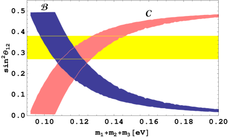
Figure 3: The solar angle $\sin^{2}\theta_{12}$ as a function of $m_{1}+m_{2}+m_{3}$ in the Model I​I. The horizontal lines shows the $3\sigma$ allowed range of the solar angle [14].

This model accommodates only the inverted mass ordering since $m_{3}$ cannot be largest among the three eigenvalues. The two eigenvalues $m_{\pm}$ are identified as $m_{2}=m_{+(-)}$ and $m_{1}=m_{-(+)}$ for $r>1\ (r<1)$ and degenerate for $r=1$. The observed mass differences are not reproduced in the regime that $|M|R\gtrsim 1/2\pi$. In such a regime, the ratio of the mass differences is given by $|\Delta m^{2}_{31}|/\Delta m^{2}_{21}\simeq-1$ for $r>1$ and $2r^{4}/s$ for $r<1$, which contradict the data.

A realistic mass pattern is obtained if the bulk Majorana scale is much smaller than the inverse of the compactification radius: $|M|R\ll 1$. In such a regime, the parameters $r$ and $|M|R$ are related as

$$\frac{m_{1}^{2}-m_{3}^{2}}{m_{2}^{2}-m_{1}^{2}}\,\simeq\,\frac{\pm r}{4\pi|M|R(r^{2}-1)},$$ (3.29)

where the plus (minus) sign in the right-hand side is for $r>1$ ($r<1$). By using (3.29), the magnitude of $\theta_{12}$ is estimated as

$$\tan 2\theta_{12}\,\simeq\,4\frac{|\Delta m^{2}_{31}|}{\Delta m^{2}_{21}}\left|\frac{r^{2}-1}{r^{2}+1}\right|.$$ (3.30)

The angle $\theta_{12}$ is zero for $r=1$ and it rapidly increases as $r$ departs from unity due to the large factor $|\Delta m^{2}_{31}|/\Delta m^{2}_{21}\simeq 30$. That is, the solar angle is small at the degenerate limit while it becomes large as the spectrum approaches the inverted hierarchy.

Figure 3 shows $\sin^{2}\theta_{12}\mathsf{}$ as a function of the total neutrino mass $\Sigma=\sum_{i}m_{i}$. The blue (shaded) region is for the category ${\cal B}$ and the pink (light-shaded) region is for ${\cal C}$. The horizontal band is the 3$\sigma$ range of $\sin^{2}\theta_{12}$ [14]. The thickness of each plot corresponds to the possible 3$\sigma$ values of $|\Delta m^{2}_{31}|/\Delta m^{2}_{21}$ in the same reference.

In the case ${\cal B}$, the solar angle is increased as the spectrum is shifted from the degenerate pattern to the hierarchical one. The 3$\sigma$ range of $\sin^{2}\theta_{12}=0.27-0.38$ is reproduced for $0.10\,{\rm eV}\lesssim\Sigma\lesssim 0.12\,{\rm eV}$, which range will be tested in the cosmological observation such as cosmic microwave background data from the Planck mission. While in the case ${\cal C}$, the solar angle is increased as the total mass is increased. This opposite behavior is because of the $45^{\circ}$ difference of the solar angle $\theta_{12}$. The predicted range of $\Sigma$ is slightly wider than the case of ${\cal B}$ and shifted to a higher region: $0.11\,{\rm eV}\lesssim\Sigma\lesssim 0.15\,{\rm eV}$.

In this model, $\theta_{13}$ and $\theta_{23}$ comes from the charged-lepton sector and their magnitudes depend on the structure of the charged-lepton mass matrix. The charged-lepton mass matrices suitable for the two options of the neutrino sector (Model I and I​I ) are discussed in the next subsection.

3.4 The charged-lepton sector

The charged-lepton sector resides on the SM boundary $y=\pi R$. The right-handed electron $e_{R}$ and the pair of muon and tauon $(\mu_{R},\tau_{R})$ are assigned to be $\underline{1}$ and $\underline{2}$, respectively. We also introduce new gauge singlet scalars $\phi_{i}$, which are assigned to be $\underline{3}$. These assignments are summarized in the table below:

	$e_{R}$	$(\mu_{R},\tau_{R})$	$(L_{e},L_{\mu},L_{\tau})$	$H$	$(\phi_{1},\phi_{2},\phi_{3})$
$S_{4}$	$\underline{1}$	$\underline{2}$	$\underline{3}$	$\underline{1}$	$\underline{3}$

For the charged leptons, the $S_{4}$ invariant Lagrangian is

$$\mathcal{L} \,=\,\frac{Y_{s}}{\Lambda}\,\overline{e_{R}}\left(L_{e}\phi_{1}+L_{\mu}\phi_{2}+L_{\tau}\phi_{3}\right)H^{*}$$

$$\,\,+\frac{Y_{d}}{\Lambda}\left[\,\left(\overline{\mu_{R}}+\overline{\tau_{R}}\right)L_{e}\phi_{1}+\left(\omega^{2}\overline{\mu_{R}}+\omega\overline{\tau_{R}}\right)L_{\mu}\phi_{2}+\left(\omega\overline{\mu_{R}}+\omega^{2}\overline{\tau_{R}}\right)L_{\tau}\phi_{3}\,\right]H^{*},$$ (3.31)

where $Y_{s}$, $Y_{d}$ are the dimensionless Yukawa couplings. After the electroweak symmetry breaking, the charged-lepton mass matrix is given by

$${M_{\ell}}=vY_{s}\begin{pmatrix}\alpha_{1}&\alpha_{2}&\alpha_{3}\\ 0&0&0\\ 0&0&0\end{pmatrix}+vY_{d}\begin{pmatrix}0&0&0\\ \alpha_{1}&\omega^{2}\alpha_{2}&\omega\alpha_{3}\\ \alpha_{1}&\omega\alpha_{2}&\omega^{2}\alpha_{3}\end{pmatrix},$$ (3.32)

where $\alpha_{i}\equiv\langle\phi_{i}\rangle/\Lambda$. The Hermitian matrix $M_{\ell}^{\dagger}M_{\ell}$ becomes

$$M_{\ell}^{\dagger}M_{\ell}=v^{2}\begin{pmatrix}\left(|Y_{s}|^{2}+2|Y_{d}|^{2}\right)\alpha_{1}^{2}&\left(|Y_{s}|^{2}-|Y_{d}|^{2}\right)\alpha_{1}\alpha_{2}&\left(|Y_{s}|^{2}-|Y_{d}|^{2}\right)\alpha_{1}\alpha_{3}\\ \left(|Y_{s}|^{2}-|Y_{d}|^{2}\right)\alpha_{1}\alpha_{2}&\left(|Y_{s}|^{2}+2|Y_{d}|^{2}\right)\alpha_{2}^{2}&\left(|Y_{s}|^{2}-|Y_{d}|^{2}\right)\alpha_{2}\alpha_{3}\\ \left(|Y_{s}|^{2}-|Y_{d}|^{2}\right)\alpha_{1}\alpha_{3}&\left(|Y_{s}|^{2}-|Y_{d}|^{2}\right)\alpha_{2}\alpha_{3}&\left(|Y_{s}|^{2}+2|Y_{d}|^{2}\right)\alpha_{3}^{2}\end{pmatrix}.$$ (3.33)

By assuming that $\alpha_{1}v\sim m_{e}$, $\alpha_{2}v\sim m_{\mu}$, $\alpha_{3}v\sim m_{\tau}$ and the Yukawa couplings are of order unity, one obtains the realistic charged-lepton masses and small mixing in (3.33). This case is suitable for Model I for the neutrino sector because the near tri-bimaximal mixing comes from the neutrino sector. Corrections from the charged-lepton mass matrix are at most ${\cal O}(m_{e}/m_{\mu})$, ${\cal O}(m_{e}/m_{\tau})$ and ${\cal O}(m_{\mu}/m_{\tau})$ for the lepton mixing angles $\theta_{12}$, $\theta_{13}$ and $\theta_{23}$, respectively.

On the other hand, the neutrino sector of Model I​I provides only $\theta_{12}$ and needs (at least) a large 2-3 mixing arising from the charged-lepton mass matrix. This is possible if $\alpha_{1}=0$ and $\alpha_{2}=\alpha_{3}=\alpha$ are realized;

$$M_{\ell}^{\dagger}M_{\ell}=v^{2}\begin{pmatrix}0&0&0\\ 0&\left(|Y_{s}|^{2}+2|Y_{d}|^{2}\right)\alpha^{2}&\left(|Y_{s}|^{2}-|Y_{d}|^{2}\right)\alpha^{2}\\ 0&\left(|Y_{s}|^{2}-|Y_{d}|^{2}\right)\alpha^{2}&\left(|Y_{s}|^{2}+2|Y_{d}|^{2}\right)\alpha^{2}\end{pmatrix}.$$ (3.34)

The charged-lepton masses and the mixing angle are

$$m_{e}^{2}=0,\quad m_{\mu}^{2}=3|Y_{d}|^{2}\alpha^{2}v^{2},\quad m_{\tau}^{2}=\left(2|Y_{s}|^{2}+|Y_{d}|^{2}\right)\alpha^{2}v^{2},\quad\theta_{23}^{\ell}=\frac{\pi}{4}.$$ (3.35)

By taking $Y_{d}/Y_{s}\simeq\sqrt{2/3}\,m_{\mu}/m_{\tau}$, one obtains the observed mass ratio $m_{\mu}/m_{\tau}$ and the large 2-3 angle which accounts for the atmospheric neutrino oscillation. For the Yukawa coupling $Y_{s}$ of order unity, $\alpha=\mathcal{O}(10^{-2})$. The nonzero electron mass is produced by holding a finite but small value of $\alpha_{1}$.

Another interesting way to obtain the realistic electron mass is to take account of the higher-order corrections to the charged-lepton mass matrix while holding the vacuum-alignment $\alpha_{1}=0$ and $\alpha_{2}=\alpha_{3}=\alpha$ strictly. The Lagrangian with the dimension six operators is given by

$$\Delta\mathcal{L} \,=\,\frac{Y_{s}^{\Delta}}{\Lambda^{2}}\overline{e_{R}}\left(\,L_{e}\phi_{2}\phi_{3}\,+\,L_{\mu}\phi_{1}\phi_{3}\,+\,L_{\tau}\phi_{1}\phi_{2}\,\right)H^{*}$$

$$\,\,+\frac{Y_{d}^{\Delta}}{\Lambda^{2}}\left[\,\left(\overline{\mu_{R}}+\overline{\tau_{R}}\right)L_{e}\phi_{2}\phi_{3}\,+\,\left(\omega^{2}\overline{\mu_{R}}+\omega\overline{\tau_{R}}\right)L_{\mu}\phi_{1}\phi_{3}\,+\,\left(\omega\overline{\mu_{R}}+\omega^{2}\overline{\tau_{R}}\right)L_{\tau}\phi_{1}\phi_{2}\,\right]H^{*}.$$ (3.36)

After $\phi_{i}$ developing the VEVs of $\langle\phi_{i}\rangle=(0,\alpha\Lambda,\alpha\Lambda)$, the charged-lepton mass matrix up to this order is written as

$$\hat{M}_{\ell}=M_{\ell}+\Delta M_{\ell}=v\begin{pmatrix}Y_{s}^{\Delta}\alpha^{2}&Y_{s}\alpha&Y_{s}\alpha\\ Y_{d}^{\Delta}\alpha^{2}&Y_{d}\omega^{2}\alpha&Y_{d}\omega\alpha\\ Y_{d}^{\Delta}\alpha^{2}&Y_{d}\omega\alpha&Y_{d}\omega^{2}\alpha\end{pmatrix}.$$ (3.37)

The Hermitian matrix $\hat{M}_{\ell}^{\dagger}\hat{M}_{\ell}$ follows

$$\hat{M}_{\ell}^{\dagger}\hat{M}_{\ell}=\alpha^{2}v^{2}\begin{pmatrix}\left(|Y_{s}^{\Delta}|^{2}+2|Y_{d}^{\Delta}|^{2}\right)\alpha^{2}&\left(Y_{s}^{\Delta}{}^{*}Y_{s}-Y_{d}^{\Delta}{}^{*}Y_{d}\right)\alpha&\left(Y_{s}^{\Delta}{}^{*}Y_{s}-Y_{d}^{\Delta}{}^{*}Y_{d}\right)\alpha\\[1.42262pt] \left(Y_{s}^{\Delta}Y_{s}^{*}-Y_{d}^{\Delta}Y_{d}^{*}\right)\alpha&|Y_{s}|^{2}+2|Y_{d}|^{2}&|Y_{s}|^{2}-|Y_{d}|^{2}\\[1.42262pt] \left(Y_{s}^{\Delta}Y_{s}^{*}-Y_{d}^{\Delta}Y_{d}^{*}\right)\alpha&|Y_{s}|^{2}-|Y_{d}|^{2}&|Y_{s}|^{2}+2|Y_{d}|^{2}\\ \end{pmatrix}.$$ (3.38)

The charged-lepton masses and mixing are given by

$$m_{e}^{2}\,\simeq\,2|Y_{d}^{\Delta}|^{2}\alpha^{4}v^{2},\qquad m_{\mu}^{2}\,\simeq\,3|Y_{d}|^{2}\alpha^{2}v^{2},\qquad m_{\tau}^{2}\,\simeq\,\left(2|Y_{s}|^{2}+|Y_{d}|^{2}\right)\alpha^{2}v^{2},$$ (3.39)

$$\theta_{12}^{\ell}=0,\qquad\theta_{13}^{\ell}\simeq\frac{\sqrt{2}\left|Y_{s}^{\Delta}Y_{s}^{*}-Y_{d}^{\Delta}Y_{d}^{*}\right|\alpha}{2|Y_{s}|^{2}+|Y_{d}|^{2}},\qquad\theta_{23}^{\ell}=\frac{\pi}{4},$$ (3.40)

where the 1-3 angle $\theta_{13}^{\ell}$ is assumed to be small not to contradict the reactor bound. As in the case of the leading-order estimation, $Y_{d}/Y_{s}\simeq\sqrt{2/3}\,m_{\mu}/m_{\tau}$ and $\alpha=\mathcal{O}(10^{-2})$ for $Y_{s}\simeq 1$. The electron mass is in the right range if $Y_{d}^{\Delta}\approx Y_{d}$. The 1-3 angle becomes $\theta_{13}^{\ell}\simeq 1/\sqrt{2}(Y_{s}^{\Delta}/Y_{s})$ which will be observable if $Y_{s}^{\Delta}/Y_{s}=\mathcal{O}(10^{-1})$.

A possible way to achieve the aligned vacuum $\langle\phi_{i}\rangle=(0,\alpha\Lambda,\alpha\Lambda)$ is to assume that the scalar fields $\phi_{i}$ propagate in the five-dimensional bulk and follow nontrivial boundary conditions [8]. By assigning the pseudotriplet $\underline{3}^{\prime}$ to $\phi_{i}$ or assuming the scalar potential to have additional $Z_{2}$ symmetry, it is possible to impose the twisted boundary condition $\phi(y+2\pi R)=-d_{2}\phi(y)$. While the first component $\phi_{1}$ cannot develop a constant VEV because of the antiperiodic boundary condition, the other two components $\phi_{2}$ and $\phi_{3}$ acquire equal VEVs since the boundary condition respects $S_{2}$ symmetry which is the exchange of the 2-3 component of the triplet $\phi_{i}$.

The bulk scalars $\phi_{i}$ with nontrivial boundary conditions are also useful for realizing a hierarchal charged-lepton mass matrix suitable for the Model I. Suppose that the right-handed charged-leptons $(e_{R},\mu_{R},\tau_{R})$ are $\underline{3}$ of $S_{4}$ and also propagate in the bulk.

The gauge singlet scalars $\phi_{i}$ are also coupled to the neutrinos via higher-dimensional operators, e.g., $\overline{\Psi}LH\phi$. For the Model I, the most stringent contribution comes from $\langle\phi_{3}\rangle$ component related to the tau mass: $m_{\tau}\simeq\sqrt{|Y_{s}|^{2}+2|Y_{d}|^{2}}v\alpha_{3}$. However, $\alpha_{3}=\mathcal{O}(10^{-2})$ if all the dimensionless couplings are of order unity. Thus the corrections from such higher-dimensional operators remain a few percent and the predictions discussed in Section 3.2 and 3.3 are valid unless the Yukawa couplings are anomalously small. A similar discussion is also hold for the Model I​I.

4 Summary

In this paper, we have examined the $S_{4}$ discrete group as a feasible candidate for the family symmetry which accounts for the leptonic generation structure. Phenomenologically viable $S_{4}$ breaking is triggered by the boundary conditions of the right-handed neutrinos which reside on the five-dimensional spacetime. With the SM fields being trapped in the four-dimensional subspace, many boundary conditions produce realistic lepton mixing slightly deviated from the tri-bimaximal mixing in a controllable way. There are two types of plausible structures (Model I and I​I in Section 3.2 and 3.3 respectively) in the neutrino sector.

In the Model I, the whole mixing matrix originates in the neutrino sector and the charged-lepton mass matrix is diagonal in a certain $S_{4}$ basis (see Appendix B). While the solar component $U_{e2}$ is robustly predicted to be $1/\sqrt{3}$, the reactor angle $\theta_{13}$ is correlated to the mass patterns. With the normal mass ordering, $\theta_{13}$ increases as the total neutrino mass decreases in such a way that $\sin\theta_{13}\gtrsim 0.07$ if $m_{1}+m_{2}+m_{3}\lesssim 0.06\,{\rm eV}$, which range will be probed at future experiments. Furthermore, the atmospheric angle $\theta_{23}$ is deviated from the maximal value $45^{\circ}$ in such a way that the deviation is ruled by the magnitude of $\theta_{13}$. While the discovery of $\theta_{13}$ is imminent for the normal mass hierarchy, the reactor angle is generally small ($\theta_{13}\lesssim 10^{-3}$) for the inverted mass ordering; the mixing matrix is predicted to be almost tri-bimaximal form in the case of the inverted ordering.

While in the Model I​I, the large solar angle $\theta_{12}$ stems from the neutrino sector and the maximal atmospheric angle $\theta_{23}$ emerges from the charged-lepton mass matrix. Unlike the Model I, the Model I​I accommodates only the inverted mass ordering. The solar angle $\theta_{12}$ is related to the total neutrino mass. Within $3\sigma$ range of the current oscillation parameters, the total mass is predicted to be in a small window $0.10\,{\rm eV}\leq m_{1}+m_{2}+m_{3}\leq 0.15\,{\rm eV}$ which can be probed by the Planck satellite. By the combined data of future oscillation experiments and cosmological observations, the models discussed here are not only tested but also distinguished each other in their predictions for the leptonic generation structure.

Besides the predictions in the masses and the mixing angles discussed in this paper, there are other phenomenological issues such as collider signals [16], leptogenesis [17], low-energy CP violation, dark matter, and so on. In particular, it might be interesting to identify some of the KK right-handed neutrinos as the dark matter by introducing the bulk Dirac masses with an appropriate choice of the parameters. These subjects remain to be explored in future work.

Acknowledgments

The authors are supported in part by the scientific grant from the ministry of education, science, sports, and culture of Japan (No. 21340055). H.I. is supported by Grand-in-Aid for Scientific Research, No.21.5817 from the Japan Society of Promotion of Science. Y.S. is supported by Grand-in-Aid for Scientific Research, No.22.3014 from the Japan Society of Promotion of Science.

Appendix A Lorentz spinors and gamma matrices

In this work, the gamma matrices are taken as

$$\{\Gamma^{M},\Gamma^{N}\}\,=\,2\eta^{MN}\,=\,2\,{\rm diag}(+1,-1,-1,-1,-1),$$ (A.1)

$$\Gamma_{\mu}=\gamma_{\mu}=\begin{pmatrix}&\sigma_{\mu}\\ \bar{\sigma}_{\mu}&\\ \end{pmatrix},\qquad i\Gamma_{4}=\gamma_{5}=\begin{pmatrix}1&\\ &-1\\ \end{pmatrix},$$ (A.2)

where $\sigma_{\mu}=(1,\sigma_{i})$ and $\bar{\sigma}_{\mu}=(1,-\sigma_{i})$. A 4-component spinor is written in terms of 2-component spinors as

$$\Psi\,=\,\begin{pmatrix}\xi_{\alpha}\\ \eta^{\dot{\alpha}}\\ \end{pmatrix}.$$ (A.3)

The Dirac and charge conjugates for $\Psi$ are given by

$$\overline{\Psi}\,=\,\big{(}\eta^{*\alpha}\;\,\xi_{\dot{\alpha}}^{*}\big{)},\qquad\quad\Psi^{c}\,=\,C_{5}\overline{\Psi}^{\rm T}\,=\,\begin{pmatrix}-\epsilon_{\alpha\beta}\eta^{*\beta}\\[1.42262pt] -\epsilon^{\dot{\alpha}\dot{\beta}}\xi^{*}_{\dot{\beta}}\,\end{pmatrix},$$ (A.4)

where $C_{5}$ is the charge conjugation matrix in five dimensions: $C_{5}=i\gamma^{2}\gamma^{0}\gamma_{5}$. The antisymmetric tensors are

$$\epsilon^{\alpha\beta}=\epsilon_{\alpha\beta}=\epsilon^{\dot{\alpha}\dot{\beta}}=\epsilon_{\dot{\alpha}\dot{\beta}}=\begin{pmatrix}&1\\ -1&\\ \end{pmatrix}.$$ (A.5)

Appendix B $S_{4}$ group

The $S_{4}$ group consists of all permutations of four objects and the order is $4!=24$. The $S_{4}$ is symmetry of the cube. The irreducible representations are two singlets $\underline{1}$ and $\underline{1}^{\prime}$, one doublet $\underline{2}$, and two triplets $\underline{3}$ and $\underline{3}^{\prime}$. In this work, we adopt the following basis [18]

$$Q=\begin{pmatrix}0&1\\ 1&0\\ \end{pmatrix},\quad P=\begin{pmatrix}\omega&0\\ 0&\omega^{2}\\ \end{pmatrix}\quad\quad(\omega\equiv e^{i\frac{2\pi}{3}})$$ (B.1)

for the doublet $\underline{2}$ and

$$Q=\begin{pmatrix}-1&0&0\\ 0&0&-1\\ 0&1&0\\ \end{pmatrix},\quad P=\begin{pmatrix}0&0&1\\ 1&0&0\\ 0&1&0\\ \end{pmatrix}$$ (B.2)

for the triplet $\underline{3}$. All the group elements are given by the products of these two generators;

$$\begin{array}[]{llll}a_{1}=Q^{4},&\quad a_{2}=Q^{2},&\quad a_{3}=PQ^{2}P^{2},&\quad a_{4}=Q^{2}PQ^{2}P^{2},\\ b_{1}=P,&\quad b_{2}=Q^{2}P,&\quad b_{3}=QPQP^{2},&\quad b_{4}=Q^{2}PQ^{2},\\ c_{1}=P^{2},&\quad c_{2}=Q^{2}P^{2},&\quad c_{3}=QPQ,&\quad c_{4}=Q^{3}PQ,\\ d_{1}=PQPQ^{2},&\quad d_{2}=PQP,&\quad d_{3}=Q^{3},&\quad d_{4}=Q,\\ e_{1}=Q^{2}PQ,&\quad e_{2}=PQ,&\quad e_{3}=Q^{3}P^{2},&\quad e_{4}=QP^{2},\\ f_{1}=QPQ^{2},&\quad f_{2}=PQP^{2},&\quad f_{3}=P^{2}Q,&\quad f_{4}=QP.\\ \end{array}$$ (B.9)

The tensor products $\underline{3}\times\underline{3}$ and $\underline{2}\times\underline{3}$ play an essential role to construct the Yukawa coupling matrices in symmetric phase. They are decomposed as $\underline{3}\times\underline{3}=\underline{1}+\underline{2}+\underline{3}+\underline{3}^{\prime}$ and $\underline{2}\times\underline{3}=\underline{3}+\underline{3}^{\prime}$. Suppose that $\psi_{i}$, $\phi_{i}$ $(i=1,2,3)$ and $\chi_{j}\,(j=1,2)$ behave as $\underline{3}$ and $\underline{2}$ under the basis of (B.2) and (B.1), respectively. Then it follows

$$\psi\times\phi = \underbrace{\sum_{i=1}^{3}\psi_{i}\phi_{i}}_{\underline{1}}+\underbrace{\left(\begin{array}[]{c}\psi_{1}\phi_{1}+\omega\psi_{2}\phi_{2}+\omega^{2}\psi_{3}\phi_{3}\\ \psi_{1}\phi_{1}+\omega^{2}\psi_{2}\phi_{2}+\omega\psi_{3}\phi_{3}\\ \end{array}\right)}_{\underline{2}}$$ (B.19)

$$\quad\quad\quad\quad+\underbrace{\left(\begin{array}[]{c}\psi_{2}\phi_{3}+\psi_{3}\phi_{2}\\ \psi_{3}\phi_{1}+\psi_{1}\phi_{3}\\ \psi_{1}\phi_{2}+\psi_{2}\phi_{1}\\ \end{array}\right)}_{\underline{3}}+\underbrace{\left(\begin{array}[]{c}\psi_{2}\phi_{3}-\psi_{3}\phi_{2}\\ \psi_{3}\phi_{1}-\psi_{1}\phi_{3}\\ \psi_{1}\phi_{2}-\psi_{2}\phi_{1}\\ \end{array}\right),}_{\underline{3}^{\prime}}$$

$$\chi\times\psi = \underbrace{\left(\begin{array}[]{c}(\chi_{1}+\chi_{2})\psi_{1}\\ (\omega^{2}\chi_{1}+\omega\chi_{2})\psi_{2}\\ (\omega\chi_{1}+\omega^{2}\chi_{2})\psi_{3}\\ \end{array}\right)}_{\underline{3}}+\underbrace{\left(\begin{array}[]{c}(\chi_{1}-\chi_{2})\psi_{1}\\ (\omega^{2}\chi_{1}-\omega\chi_{2})\psi_{2}\\ (\omega\chi_{1}-\omega^{2}\chi_{2})\psi_{3}\\ \end{array}\right).}_{\underline{3}^{\prime}}$$ (B.26)

References

• [1] For review, R.N. Mohapatra et al., Rept. Prog. Phys.  70 (2007) 1757; A. Strumia and F. Vissani, hep-ph/0606054; M.C. Gonzalez-Garcia and M. Maltoni, Phys. Rept.  460 (2008) 1.
• [2] P.F. Harrison, D.H. Perkins and W.G. Scott, Phys. Lett.  B 530 (2002) 167; P.F. Harrison and W.G. Scott, Phys. Lett.  B 535 (2002) 163.
• [3] S. Pakvasa and H. Sugawara, Phys. Lett. B 73 (1978) 61; H. Harari, H. Haut and J. Weyers, Phys. Lett. B 78 (1978) 459; Y. Koide, Phys. Rev. D 28 (1983) 252; M. Tanimoto, Phys. Rev.  D 41 (1990) 1586; C. E. Lee, C. L. Lin and Y. W. Yang, “The minimal extension of the standard model with S(3) symmetry,” Prepared for 2nd International Spring School on Medium and High-energy Nuclear Physics, Taipei, Taiwan, 8-12 May 1990; H. Fritzsch and J. Plankl, Phys. Lett. B 237 (1990) 451; L.J. Hall and H. Murayama, Phys. Rev. Lett. 75 (1995) 3985; K. Kang, J. E. Kim and P. Ko, Z. Phys.  C 72 (1996) 671; K. Kang, S. K. Kang, J. E. Kim and P. Ko, Mod. Phys. Lett.  A 12 (1997) 1175; M. Fukugita, M. Tanimoto and T. Yanagida, Phys. Rev. D 57 (1998) 4429; R.N. Mohapatra and S. Nussinov, Phys. Lett. B 441 (1998) 299; M. Tanimoto, Phys. Rev.  D 59 (1999) 017304; M. Tanimoto, T. Watari and T. Yanagida, Phys. Lett.  B 461 (1999) 345; Y. Koide, Phys. Rev.  D 60 (1999) 077301; M. Tanimoto, Phys. Lett.  B 483 (2000) 417; R. Dermisek and S. Raby, Phys. Rev. D 62 (2000) 015007.
• [4] E. Ma and G. Rajasekaran, Phys. Rev.  D 64 (2001) 113012; E. Ma, Mod. Phys. Lett.  A 17 (2002) 2361; K. S. Babu, T. Enkhbat and I. Gogoladze, Phys. Lett.  B 555 (2003) 238; K. S. Babu, E. Ma and J. W. F. Valle, Phys. Lett.  B 552 (2003) 207; K. S. Babu, T. Kobayashi and J. Kubo, Phys. Rev.  D 67 (2003) 075018; E. Ma, Phys. Rev.  D 70 (2004) 031901; M. Hirsch, J. C. Romao, S. Skadhauge, J. W. F. Valle and A. Villanova del Moral, Phys. Rev.  D 69 (2004) 093006; G. Altarelli and F. Feruglio, Nucl. Phys.  B 720 (2005) 64; S. L. Chen, M. Frigerio and E. Ma, Nucl. Phys.  B 724 (2005) 423; A. Zee, Phys. Lett.  B 630 (2005) 58; G. Altarelli and F. Feruglio, Nucl. Phys.  B 741 (2006) 215; For more recent references, see the papers cited in H. Ishimori, T. Kobayashi, H. Ohki, H. Okada, Y. Shimizu and M. Tanimoto, Prog. Theor. Phys. Suppl.  183 (2010) 1; G. Altarelli and F. Feruglio, arXiv:1002.0211.
• [5] Y. Yamanaka, H. Sugawara and S. Pakvasa, Phys. Rev.  D 25 (1982) 1895 [Erratum-ibid.  D 29 (1984) 2135]; T. Brown, S. Pakvasa, H. Sugawara and Y. Yamanaka, Phys. Rev.  D 30 (1984) 255; T. Brown, N. Deshpande, S. Pakvasa and H. Sugawara, Phys. Lett.  B 141 (1984) 95; E. Ma, Phys. Lett.  B 632 (2006) 352; C. Hagedorn, M. Lindner and R. N. Mohapatra, JHEP 0606 (2006) 042; Y. Cai and H. B. Yu, Phys. Rev.  D 74 (2006) 115005; H. Zhang, Phys. Lett.  B 655 (2007) 132; Y. Koide, JHEP 0708 (2007) 086; C. S. Lam, Phys. Rev.  D 78 (2008) 073015; F. Bazzocchi and S. Morisi, Phys. Rev.  D 80 (2009) 096005; H. Ishimori, Y. Shimizu and M. Tanimoto, Prog. Theor. Phys.  121 (2009) 769; F. Bazzocchi, L. Merlo and S. Morisi, Nucl. Phys.  B 816 (2009) 204; Phys. Rev.  D 80 (2009) 053003; G. Altarelli, F. Feruglio and L. Merlo, JHEP 0905 (2009) 020; W. Grimus, L. Lavoura and P. O. Ludl, J. Phys. G 36 (2009) 115007; G. J. Ding, Nucl. Phys.  B 827 (2010) 82; B. Dutta, Y. Mimura and R. N. Mohapatra, JHEP 1005 (2010) 034; D. Meloni, arXiv:0911.3591; C. Hagedorn, S. F. King and C. Luhn, JHEP 1006 (2010) 048; R. de Adelhart Toorop, F. Bazzocchi and L. Merlo, JHEP 1008 (2010) 001; H. Ishimori, K. Saga, Y. Shimizu and M. Tanimoto, Phys. Rev.  D 81 (2010) 115009; G. J. Ding, arXiv:1006.4800; P. V. Dong, H. N. Long, D. V. Soa and V. V. Vien, arXiv:1009.2328.
• [6] J. Scherk and J.H. Schwarz, Phys. Lett.  B 82 (1979) 60; Nucl. Phys.  B 153 (1979) 61.
• [7] N. Haba, A. Watanabe and K. Yoshioka, Phys. Rev. Lett.  97 (2006) 041601.
• [8] T. Kobayashi, Y. Omura and K. Yoshioka, Phys. Rev.  D 78 (2008) 115006.
• [9] N. Arkani-Hamed, S. Dimopoulos and G.R. Dvali, Phys. Lett.  B 429 (1998) 263; I. Antoniadis, N. Arkani-Hamed, S. Dimopoulos and G.R. Dvali, Phys. Lett.  B 436 (1998) 257.
• [10] L. Randall and R. Sundrum, Phys. Rev. Lett. 83 (1999) 3370; ibid. 83 (1999) 4690.
• [11] K.R. Dienes, E. Dudas and T. Gherghetta, Nucl. Phys. B 557 (1999) 25; N. Arkani-Hamed, S. Dimopoulos, G.R. Dvali and J. March-Russell, Phys. Rev. D 65 (2002) 024032.
• [12] A. Lukas, P. Ramond, A. Romanino and G.G. Ross, JHEP 0104 (2001) 010.
• [13] A. Watanabe and K. Yoshioka, Phys. Lett.  B 683 (2010) 289; arXiv:1007.1527.
• [14] T. Schwetz, M. A. Tortola and J. W. F. Valle, New J. Phys.  10 (2008) 113011.
• [15] Takashi Kobayashi (KEK), “Status of T2K”, Talk at Neutrino 2010, June 14-19, 2010, Athens, Greece, http://www.neutrino2010.gr/ ; Anatael Cabrera, “Status of the DOUBLE CHOOZ Reactor Experiment” , Talk at Neutrino 2010, June 14-19, 2010, Athens, Greece. http://www.neutrino2010.gr/ ; Meng Wang,“Status of the Daya Bay Reactor Neutrino Experiment”, Talk at Neutrino 2010, June 14-19, 2010, Athens, Greece. http://www.neutrino2010.gr/ ; KyungKwang Joo, “17:10 Status of the RENO Reactor Neutrino Experiment”, Talk at Neutrino 2010, June 14-19, 2010, Athens, Greece. http://www.neutrino2010.gr/ .
• [16] N. Haba, S. Matsumoto and K. Yoshioka, Phys. Lett.  B 677 (2009) 291; M. Blennow, H. Melbeus, T. Ohlsson and H. Zhang, arXiv:1003.0669; S. Matsumoto, T. Nabeshima and K. Yoshioka, arXiv:1004.3852; T. Saito et al., arXiv:1008.2257.
• [17] A. Pilaftsis, Phys. Rev.  D 60 (1999) 105023; A.D. Medina and C.E.M. Wagner, JHEP 0612 (2006) 037; T. Gherghetta, K. Kadota and M. Yamaguchi, Phys. Rev.  D 76 (2007) 023516; P.H. Gu, Phys. Rev.  D 81 (2010) 073002.
• [18] H. Ishimori, T. Kobayashi, H. Ohki, H. Okada, Y. Shimizu and M. Tanimoto, in Ref. [4].