Supplementary Material for
 
Dynamic reconfiguration of human brain networks during learning

¹Complex Systems Group, Department of Physics, University of California, Santa Barbara, CA 93106, USA
²Department of Psychology and UCSB Brain Imaging Center, University of California, Santa Barbara, CA 93106, USA
³Oxford Centre for Industrial and Applied Mathematics, Mathematical Institute, University of Oxford, Oxford OX1 3LB, UK
⁴CABDyN Complexity Centre, University of Oxford, Oxford OX1 1HP, UK
⁵Carolina Center for Interdisciplinary Applied Mathematics, Department of Mathematics, University of North Carolina at Chapel Hill, NC 27599, USA
⁶Institute for Advanced Materials, Nanoscience & Technology, University of North Carolina, Chapel Hill, NC 27599, USA

Full Description of Methods

Sample

Twenty-five right-handed participants (16 female, 9 male) volunteered with informed consent in accordance with the Institutional Review Board/Human Subjects Committee, University of California, Santa Barbara. Handedness was determined by the Edinburgh Handedness Inventory. The mean age of the participants was 24.25 years (range 18.5–30 years). Of these, 2 participants were removed because their task accuracy was less than 60% correct, 1 was removed because of a cyst in presupplementary motor area (preSMA), and 4 were removed for shortened scan sessions. This left 18 participants in total. All participants had less than 4 years of experience with any one musical instrument, had normal vision, and had no history of neurological disease or psychiatric disorders. Participants were paid for their participation. All participants completed 3 training sessions in a 5-day period, and each session was performed inside the Magnetic Resonance Imaging (MRI) scanner.

Experimental Setup and Procedure

Participants were placed in a supine position in the MRI scanner. Padding was placed under the knees in order to maximize comfort and provide an angled surface to position the stimulus response box. Padding was placed under the left forearm to minimize muscle strain when participants typed sequences. Finally, in order to minimize head motion, padded wedges were inserted between the participant and head coil of the MRI scanner. For all sessions, participants performed a cued sequence production (CSP) task (see Figure S1), responding to visually cued sequences by generating responses using their non-dominant (left) hand on a custom fiber-optic response box. For some participants, a small board was placed between the response box and the lap in order to help balance the box effectively. Responses were made using the 4 fingers of the left hand (the thumb was excluded). Visual cues were presented as a series of musical notes on a 4-line music staff. The notes were reported in a manner that mapped the top line of the staff to the leftmost key depressed with the pinkie finger and so on, so that notes found on the bottom line mapped onto the rightmost key with the index finger (Figure S1B). Each 12-element note sequence contained 3 notes per line, which were randomly ordered without repetition and free of regularities such as trills (e.g., 121) and runs (e.g., 123). The number and order of sequence trials was identical for all participants.

A trial began with the presentation of a fixation signal, which was displayed for $2$ sec. The complete 12-element sequence was presented immediately following the removal of the fixation, and participants were then instructed to respond as soon as possible. They were given a period of 8 sec to type each sequence correctly. Participants trained on a set of 16 unique sequences, and there were three different levels of training exposure. Over the course of the three training sessions, three sequences—known as skilled sequences—were presented frequently, with 189 trials for each sequence. A second set of three sequences, termed familiar sequences, were presented for 30 trials each throughout training. A third set composed of 10 different sequences, known as novice sequences, were also presented; each novice sequence was presented 4–8 times during training.

Skilled and familiar sequences were practiced in blocks of 10 trials, so that 9 out of 10 trials were composed of the same sequence and 1 of the trials contained a novice sequence. If a sequence was reported correctly, then the notes were immediately removed from the screen and replaced with the fixation signal, which remained on the screen until the trial duration (8 sec) was reached. If there were any incorrect movements, then the sequence was immediately replaced with the verbal cue INCORRECT and participants subsequently waited for the start of the next trial. Trials were separated with an inter-trial interval (ITI) lasting between 0 sec and 20 sec, not including any time remaining from the previous trial. Following the completion of each block, feedback (lasting 12 sec and serving as a rest) was presented that detailed the number of correct trials and the mean time that was taken to complete a sequence. Training epochs contained 40 trials (i.e., 4 blocks) and lasted a total of 345 scan repetition times (TRs), which took a total of 690 sec. There were 6 scan epochs per training session (2070 scan TRs). In total, each skilled sequence was presented 189 times over the course of training (18 scan epochs; 6210 TRs).

In order to familiarize participants with the task, they were given a short series of warm-up trials the day before the initial training session inside the scanner. Practice was also given in the scanner during the acquisition of the structural scans and just prior to the start of the first training-session epoch. Stimulus presentation was controlled with MATLAB^® version 7.1 (Mathworks, Natick, MA) in conjunction with Cogent 2000 (Functional Imaging Laboratory, 2000). Key-press responses and response times were collected using a fiber-optic custom button box transducer that was connected to a digital response card (DAQCard-6024e; National Instruments, Austin, TX). We assessed learning using the slope of the movement time (MT), which is the difference between the time of the first button press and the time of the last button press in a single sequence (see Figure S1B)[1]. The negative slope of the movement curve over trials indicates that learning is occurring[1].

Acquisition and Preprocessing of fMRI Data

Functional MRI (fMRI) recordings were conducted using a 3.0 T Siemens Trio with a 12-channel phased-array head coil. For each functional run, a single-shot echo planar imaging that is sensitive to blood oxygen level dependant (BOLD) contrast was used to acquire 33 slices (3 mm thickness) per repetition time (TR), with a TR of 2000 ms, an echo time (TE) of 30 ms, a flip angle of 90 degrees, and a field of view (FOV) of 192 mm. The spatial resolution of the data was defined by a 64 $\times$ 64 acquisition matrix. Before the collection of the first functional epoch, a high-resolution T1-weighted sagittal sequence image of the entire brain was acquired (TR = 15.0 ms, TE = 4.2 ms, flip angle = 9 degrees, 3D acquisition, FOV = 256 mm; slice thickness = 0.89 mm, and spatial acquisition matrix dimensions = 256 $\times$ 256).

All image preprocessing was performed using the FMRIB (Oxford Centre for Functional Magnetic Resonance Imaging of the Brain) Software Library (FSL) [2]. Motion correction was performed using the program MCFLIRT (Motion Correction using FMRIB’s Linear Image Registration Tool). Images were high-pass filtered with a 50 sec cutoff period. Spatial smoothing was performed using a kernel where the full width at half maximum was 8 mm. No temporal smoothing was performed. The signals were normalized globally to account for transient fluctuations in signal intensity.

Partitioning the Brain into Regions of Interest

Brain function is characterized by a spatial specificity: different portions of the cortex emit inherently different activity patterns that depend on the experimental task at hand. In order to measure the functional connectivity between these different portions, it is common to apply an atlas of the entire brain to raw fMRI data in order to combine information from all 3 mm cubic voxels found in a given functionally or anatomically defined region (for recent reviews, see [3, 4, 5]). Several atlases are currently available, and each provides slightly different parcellations of the cortex into discrete volumes of interest. Several recent studies have highlighted the difficulty of comparing results from network analyses derived from different atlases [6, 7, 8]. In the present work, we have therefore used a single atlas that provides the largest number of uniquely identifiable regions—this is the Harvard-Oxford (HO) atlas, which is available through the FSL toolbox [2, 9]. The HO atlas provides 112 functionally and anatomically defined cortical and subcortical regions; for a list of the brain regions, see Supplementary Table 1. Therefore, for each individual fMRI data set, we estimated regional mean BOLD time series by averaging voxel time series in each of the 112 regions. Each regional mean time series was composed of 2070 time points for each of the 3 experimental sessions (for a total of 6210 time points for the complete experiment).

Wavelet Decomposition

Brain function is also characterized by a frequency specificity; different cognitive and physiological functions are associated with different frequency bands, which can be investigated using wavelets. Wavelet decompositions of fMRI time series have been applied extensively in both resting-state and task-based conditions [10, 11]. In both cases, they provide increased sensitivity for the detection of small signal changes in non-stationary time series with noisy backgrounds [12]. In particular, the maximum-overlap discrete wavelet transform (MODWT) has been extensively used in connectivity investigations of fMRI [13, 14, 15, 16, 17, 18]. Accordingly, we used MODWT to decompose each regional time series into wavelet scales corresponding to specific frequency bands [19]. We were interested in quantifying high-frequency components of the fMRI signal, correlations between which might be indicative of cooperative temporal dynamics of brain activity during a task. Because our sampling frequency was 2 sec (1 TR = 2 sec), wavelet scale one provided information on the frequency band 0.125–0.25 Hz and wavelet scale two provided information on the frequency band 0.06–0.125 Hz. Previous work has indicated that functional associations between low-frequency components of the fMRI signal (0–0.15 Hz) can be attributed to task-related functional connectivity, whereas associations between high-frequency components (0.2–0.4 Hz) cannot [20]. This frequency specificity of task-relevant functional connectivity is likely to be due at least in part to the hemodynamic response function, which might act as a noninvertible bandpass filter on underlying neural activity [20]. In the present study, we therefore restricted our attention to wavelet scale two in order to assess dynamic changes in task-related functional brain architecture over short time scales while retaining sensitivity to task-perturbed endogenous activity [21], which is most salient at about 0.1 Hz [22, 23, 24].

Connectivity Over Multiple Temporal Scales

Multiscale Connectivity Estimation

We measured functional connectivity over three temporal scales: the large scale of the complete experiment (which lasted 3 hours and 27 minutes), the session time scale of each fMRI recording session (3 sessions of 69 minutes each; each session corresponded to 2070 time points), and the shorter time scales of intra-session time windows (where each time window was approximately 3.5 min long and lasted 80 time points).

In the investigation of large-scale connectivity, we concatenated regional mean time series over all 3 sessions, as has been done previously [25]. We then constructed for each subject a functional association matrix based on correlations between regional mean time series. At the mesoscopic scale, we extracted regional mean time series from each experimental session separately to compute session-specific matrices. At the small scale, we constructed intra-session time windows with a length of $T=80$ time points, giving a total of 25 time windows in each session (see the Results section of this supplementary document for a detailed investigation across a range of $T$ values). We constructed separate functional association matrices for each subject in each time window (25) for each session (3) for a total of 75 matrices per subject. We chose the length of the time window to be long enough to allow adequate estimation of correlations over the frequencies that are present in the wavelet band of interest (0.06–0.12 Hz), yet short enough to allow a fine-grained measurement of temporal evolution over the full experiment.

Construction of Brain Networks

To construct a functional network, we must first define a measure of functional association between regions. Measures of functional association range from simple linear correlation to nonlinear measures such as mutual information. In the majority of network investigations in fMRI studies to date, the measure of choice has been the Pearson correlation[13, 15, 26, 27, 18], perhaps due to its simplicity and ease of interpretation. Therefore, in order to estimate static functional association, we calculated the Pearson correlation between the regional mean time series of all possible pairs of regions $i$ and $j$. This yields an $N\times N$ correlation matrix with elements $r_{i,j}$, where $N=112$ is the number of brain regions of interest in the full brain atlas (see earlier section on “Partitioning the Brain into Regions of Interest” for further details).

However, as pointed out in other network studies of fMRI data[13], not all elements $r_{i,j}$ of the full correlation matrix necessarily indicate significant functional relationships. Therefore, in addition to the correlation matrix element $r_{i,j}$, we computed the $p$-value matrix element $p_{i,j}$, which give the probabilities of obtaining a correlation as large as the observed value $r_{i,j}$ by random chance when the true correlation is zero. We estimated $p$-values using approximations based on the $t$-statistic using the MATLAB^® function corrcoef[28]. In the spirit of Ref. [29] and following Ref. [13], we then tested the $p$-values $p_{i,j}$ for significance using a False Discovery Rate (FDR) of $p<0.05$ to correct for multiple comparisons[30, 31]. We retained matrix elements $r_{i,j}$ whose $p$-values $p_{i,j}$ passed the statistical FDR threshold. Elements of $r_{i,j}$ whose $p$-values $p_{i,j}$ did not pass the FDR threshold were set to zero in order to create new correlation matrix elements $r^{\prime}_{i,j}$.

We applied the statistical threshold to all $r_{i,j}$ independent of the sign of the correlation. Therefore, the resulting $r^{\prime}_{i,j}$ could contain both positive and negative elements if there existed both positive and negative elements of $r_{i,j}$ whose $p$-values $p_{i,j}$ passed the FDR threshold. Because this was a statistical threshold, the network density of $r^{\prime}_{i,j}$ (defined as the fraction of non-zero matrix elements) was determined statistically rather than being set a priori. Network density varied over temporal resolutions; the mean density and standard deviation for networks derived from correlation matrices at the largest time scale (3 hr and 27 minutes) was 0.906 (0.019%), at the intermediate time scale (69 min) was 0.846 (0.029), and at the short time scale (3.5 min) was 0.423 (0.110).

We performed the procedure described above for each subject separately to create subject-specific corrected correlation matrices. These statistically corrected matrices gave adjacency matrices $\mathbf{A}$ (see the discussion below) whose elements were $A_{ij}=r^{\prime}_{i,j}$.

Network Modularity

To characterize the large-scale functional organization of the subject-specific weighted matrices $\mathbf{A}$, we used tools from network science [32]. In a network framework, brain regions constitute the nodes of the network, and inter-regional functional connections that remain in the connectivity matrix constitute the edges of the network. One powerful concept in the study of networks is that of community structure, which can be studied using algorithmic methods [33, 34]. Community detection is an attempt to decompose a system into subsystems (called ‘modules’ or ‘communities’). Intuitively, a module consists of a group of nodes (in our case, brain regions) that are more connected to one another than they are to nodes in other modules. A popular way to investigate community structure is to optimize the partitioning of nodes into modules such that the quality function $Q$ is maximized (see [33, 34] for recent reviews and [35] for a discussion of caveats), for which we give a formula below.

From a mathematical perspective, the quality function $Q$ is simple to define. One begins with a graph composed of $N$ nodes and some set of connections between those nodes. The adjacency matrix $\mathbf{A}$ is then an $N\times N$ matrix whose elements $A_{ij}$ detail a direct connection or ‘edge’ between nodes $i$ and $j$, with a weight indicating the strength of that connection. The quality of a hard partition of $\mathbf{A}$ into communities (whereby each node is assigned to exactly one community) is then quantified using the quality function $Q$. Suppose that node $i$ is assigned to community $g_{i}$ and node $j$ is assigned to community $g_{j}$. The most popular form of the quality function takes the form [33, 34]

$$Q=\sum_{ij}[A_{ij}-P_{ij}]\delta(g_{i},g_{j})\,,$$ (1)

where $\delta(g_{i},g_{j})=1$ if $g_{i}=g_{j}$ and it equals $0$ otherwise, and $P_{ij}$ is the expected weight of the edge connecting node $i$ and node $j$ under a specified null model. (The specific choice of $Q$ in Equation 1 is called the network modularity or modularity index [36].) A most common null model (by far) used for static network community detection is given by [33, 34, 37]

$$P_{ij}=\frac{k_{i}k_{j}}{2m}\,,$$ (2)

where $k_{i}$ is the strength of node $i$, $k_{j}$ is the strength of node $j$, and $m=\frac{1}{2}\sum_{ij}A_{ij}$. The maximization of the modularity index $Q$ gives a partition of the network into modules such that the total edge weight inside of modules is as large as possible (relative to the null model, subject to the limitations of the employed computational heuristics, as optimizing $Q$ is NP-hard [33, 34, 38]).

Network modularity has been used recently for investigations of resting-state functional brain networks derived from fMRI [26, 27] and of anatomical brain networks derived from morphometric analyzes [39]. In these previous studies, brain networks were constructed as undirected binary graphs, so that each edge had a weight of either $1$ or $0$. The characteristics of binary graphs derived from neuroimaging data are sensitive to a wide variety of cognitive, neuropsychological, and neurophysiological factors [4, 5]. However, increased sensitivity is arguably more likely in the context of the weighted graphs that we consider, as they preserve the information regarding the strength of functional associations (though, as discussed previously, matrix elements $r_{i,j}$ that are statistically insignificant are still set to $0$) [40]. An additional contrast between previous studies and the present one is that (to our knowledge) investigation of network modularity has not yet been applied to task-based fMRI experiments, in which modules might have a direct relationship with goal-directed function.

We partitioned the networks represented by the weighted connectivity matrices into $n$ communities by using a Louvain greedy community detection method [41] to optimize the modularity index $Q$. Because the edge weights in the correlation networks that we constructed contain both positive and negative correlation coefficients, we used the signed null model proposed in Ref. [42] to account for communities of nodes associated with one another through both negative and positive edge weights. (Recall that we are presently discussing aggregated correlation networks $A$, so we are detecting communities in single-layer networks, as has been done in previous work. In order to investigate time-evolving communities, we will later employ a new mathematical development that makes it possible to perform community detection in multilayer networks[43].) We first defined $w_{ij}^{+}$ to be an $N\times N$ matrix containing the positive elements of $A_{ij}$ and $w_{ij}^{-}$ to be an $N\times N$ matrix containing only the negative elements of $A_{ij}$. The quality function to be maximized is then given by

$$Q_{\pm}=\frac{1}{2w^{+}+2w^{-}}\sum_{i}\sum_{j}\left[A_{ij}-\left(\gamma^{+}\frac{w_{i}^{+}w_{j}^{+}}{2w^{+}}-\gamma^{-}\frac{w_{i}^{-}w_{j}^{-}}{2w^{-}}\right)\right]\delta(g_{i}g_{j})\,,$$ (3)

where $g_{i}$ is the community to which node $i$ is assigned, $g_{j}$ is the community to which node $j$ is assigned, $\gamma^{+}$ and $\gamma^{-}$ are resolution parameters, and $w_{i}^{+}=\sum_{j}w_{ij}^{+}$, $w_{i}^{-}=\sum_{j}w_{ij}^{-}$ [42]. For simplicity, we set the resolution parameter values to unity.

In our investigation, we have focused on the mean properties of ensembles of partitions rather than on detailed properties of individual partitions. This approach is consistent with recent work illustrating the fact that the optimization of quality functions like $Q$ and $Q_{\pm}$ is hampered by the complicated shape of the optimization landscape. In particular, one expects to find a large number of partitions with near-optimum values of the quality function [35], collectively forming a high-modularity plateau. Theoretical work estimates that the number of “good” (in the sense of high values of $Q$ and similar quality functions) partitions scales as $2^{\bar{n}-1}$, where $\bar{n}$ is the mean number of modules in a given partition [35]. In both toy networks and networks constructed from empirical data, many of the partitions found by maximizing a quality function disagree with one another on the components of even the largest module, impeding interpretations of particular partitions of a network [35]. Therefore, in the present work, we have focused on quantifying mean qualities of the partitions after extensive sampling of the high-modularity plateau. Importantly, the issue of extreme near-degeneracy of quality functions like $Q$ is expected to be much less severe in the networks that we consider than is usually the case, because we are examining small, weighted networks rather than large, unweighted networks [35]. We further investigate the degenerate solutions in terms of their mean, standard deviation, and maximum. We find that $Q_{\pm}$ values are tightly distributed, with maximum values usually less than three standard deviations from the mean (see Supplementary Results).

Statistical Testing

To determine whether the value of $Q_{pm}$ or the number of modules was greater or less than expected in a random system, we constructed randomized networks with the same degree distribution as the true brain networks. As has been done previously[44, 27], we began with a real brain network and then iteratively rewired it using the rewiring algorithm of Maslov and Sneppen [45]. The procedure we used for accomplishing this rewiring was to choose at random two edges—one that connects node A to node B and another that connects nodes C and D—and then to rewire them to connect A to C and B to D. This allows us to preserve the degree, or number of edges, emanating from each node although it does not retain a node’s strength. To ensure a thorough randomization of the underlying connectivity structure, we performed this procedure multiple times, such that the expected number of times that each edge was ‘rewired’ was 20. This null model will be hereafter referred to as the static random network null model. (This is distinct from the null models that we have developed for statistical testing of community structure in multilayer networks, as discussed in the main manuscript and in later sections of this Supplement.) The motivation for this process is to compare the brain with a null model that resembles the configuration model [46], which is a random graph with prescribed degree distribution.

We constructed 100 instantiations of the static random network null model for each real network that we studied. We constructed representative values for diagnostics from the random networks by taking the mean network modularity and mean number of modules over those 100 random networks. We then computed the difference between the representative random values and the real values for each diagnostic, and we performed a one-sample $t$-test over subjects to determine whether that difference was significantly greater than or less than zero. For each case, we then reported $p$-values for these tests.

Sampling of the static random network null model distribution is important in light of the known degeneracies of modularity (which we discuss further in the Supplementary Results section below) [35]. One factor that accounts for a significant amount of variation in $Q_{\pm}$ is the size (i.e., number of nodes) of the network, so comparisons between networks of different sizes must be performed with caution. Therefore, we note that all networks derived from the aforementioned null model retain both the same number of nodes and the same number of edges as the real networks under study. This constrains important factors in the estimation of $Q_{\pm}$.

Visualization of Networks

We visualized networks using the software package MATLAB^® (2007a, The MathWorks Inc., Natick, MA). Following Ref. [47], we used the Fruchtermann-Reingold algorithm [48] to determine node placement for a given network with respect to the extracted communities and then used the Kamada-Kawai algorithm [49] to place the nodes within each community.

Multilayer Network Modularity: Temporal Dynamics of Intra-Session Connectivity

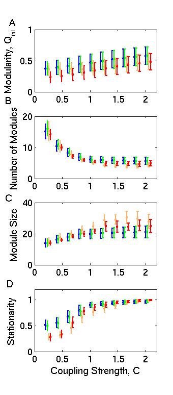
Figure 3: Effects of the coupling parameter $C$ on the four diagnostics in this study: modularity index $Q_{ml}$, number of modules $n$, module size (i.e., number of nodes) $s$, and module stationarity $\zeta$. We first averaged values over 100 ‘optimal’ partitions (see the discussion in the text), so this figure gives mean values of all diagnostics. The error bars indicate standard deviations over subjects and sessions. Colors indicate network type: cortical network (blue), temporal null model network (green), nodal null model network (orange), and connectional null model network (red). Error bars for different network types at a given value of $C$ (0.2, 0.4, 0.6, 0.8, 1, 1.2, 1.4, 1.6, 1.8, 2) are offset from each other for better visualization.

In order to investigate the temporal evolution of modular architecture in human functional connectivity, we used a mutilayer network framework in which each layer consists of a network derived from a single time window. Networks in consecutive layers therefore correspond to consecutive time windows. We linked networks in consecutive time windows by connecting each node in one window to itself in the previous and in the next windows (as shown in Figure 3A-B in the main text) [43]. We constructed a multilayer network for each individual and in each of the three experimental sessions. We then performed community detection by optimizing a multilayer modularity (see the discussion below) [43] using the Louvain greedy algorithm (suitably adapted for this more general structure) on each multilayer network in order to assess the modular architecture in the temporal domain.

Our examination of static network architecture, we used the wavelet correlation to assess functional connectivity. Unfortunately, more sensitive measures of temporal association such as the spectral coherence are not appropriate over the long time scales assessed in the static investigation due to the nonstationarity of the fMRI time series[10, 11, 12], and it is exactly for this reason that we have used the wavelet correlation for the investigation of aggregated (static) networks. However, over short temporal scales such as those being used to construct the multilayer networks, fMRI signals in the context of the motor learning task that we study can be assumed to be stationary[50], so spectral measures such as the coherence are potential candidates for the measurement of functional association.

In the examination of the dynamic network architecture of brain function using multilayer community detection, our goal was to measure temporal adaptivity of modular function over short temporal scales. In order to estimate that temporal adaptivity with enhanced precision, we used the magnitude squared spectral coherence (as estimated using the minimum-variance distortionless response method [51]) as a measure of nonlinear functional association between any two time series. In using the coherence, which has been demonstrated to be useful in the context of fMRI neuroimaging data [20], we were able to measure frequency-specific linear relationships between time series.

As in the static network analysis described earlier, we tested the elements of each $N\times N$ coherence matrix (which constitutes a single layer) for significance using an FDR correction for multiple comparisons. We used the original weighted (coherence values) of network links corresponding to the elements that passed this statistical test, while those corresponding to elements that did not pass the test were set to zero. In applying a community detection technique to the resulting coherence matrices, it is important to note that the coherence is bounded between $0$ and $1$. We can therefore use a multilayer quality function with an unsigned null model rather than the signed null model used in the static case described earlier. The multilayer modularity $Q_{ml}$ is given by [43]

$$Q_{ml}=\frac{1}{2\mu}\sum_{ijlr}\left\{\left(A_{ijl}-\gamma_{l}\frac{k_{il}k_{jl}}{2m_{l}}\right)\delta_{lr}+\delta_{ij}C_{jlr}\right\}\delta(g_{il},g_{jr})\,,$$ (4)

where the adjacency matrix of layer $l$ (i.e., time window number $l$) has components $A_{ijl}$, $\gamma_{l}$ is the resolution parameter of layer $l$, $g_{il}$ gives the community assignment of node $i$ in layer $l$, $g_{jr}$ gives the community assignment of node $j$ in layer $r$, $C_{jlr}$ is the connection strength between node $j$ in layer $r$ and node $j$ in layer $l$ (see the discussion below), $k_{il}$ is the strength of node $i$ in layer $l$, $2\mu=\sum_{jr}\kappa_{jr}$, $\kappa_{jl}=k_{jl}+c_{jl}$, and $c_{jl}=\sum_{r}C_{jlr}$. For simplicity, as in the static network case, we set the resolution parameter $\gamma_{l}$ to unity and we have set all non-zero $C_{jlr}$ to a constant $C$, which we will term the ‘inter-layer coupling’. In the main manuscript, we report results for $C=1$. In the Supplementary Results section of this document, we investigate the dependence of our results on alternative choices for the value of $C$.

Diagnostics

We used several diagnostics to characterize dynamic modular structure. These include the multilayer network modularity $Q_{ml}$, the number of modules $n$, the module size $s$, and the stationarity of modules $\zeta$. We defined the size of a module $s$ to be the mean number of nodes per module over all time windows over which the community exists. We used the definition of module stationarity from Ref. [52]. We started by calculating the autocorrelation function $U(t)$ of two states of the same community $G(t)$ at $t=1$ time steps apart using the formula

$$U(t)\equiv\frac{|G(t_{0})\cap G(t_{0}+t)|}{|G(t_{0})\cup G(t_{0}+t)|}\,,$$ (5)

where $t_{0}$ is the time at which the community is born, $|G(t_{0})\cap G(t_{0}+t)|$ is the number of nodes that are members of both $G(t_{0})$ and $G(t_{0}+t)$, and $|G(t_{0})\cup G(t_{0}+t)|$ is the total number of nodes in the union of $G(t_{0})$ and $G(t_{0}+t)$ [52]. We defined $t^{\prime}$ to be the final time step before the community is extinguished. The stationarity of a community is then given by

$$\zeta\equiv\frac{\sum_{t=t_{0}}^{t^{\prime}-1}U(t,t+1)}{t^{\prime}-t_{0}-1}\,,$$ (6)

which is the mean autocorrelation over consecutive time steps [52].

Statistical Framework

The study of the “modular architecture” of a system is of little value if the system is not modular. It is therefore imperative to statistically quantify the presence or absence of modular architecture to justify the use of community detection in a given application. Appropriate random null models have been developed and applied to the static network framework [44, 27], but no such null models yet exist for the multilayer framework. We therefore developed several null models in order to statistically test the temporal evolution of modular structure. We constructed three independent null models to test for (1) network structure dependent on the topological architecture of connectivity, (2) network structure dependent on nodal identity, and (3) network structure dependent on the temporal organization of layers in the multilayer framework.

In the connectional null model (1), we scrambled links between nodes in any given time window (the entire experiment, 3.45 hr; the individual scanning session, 69 min; or intra-session time windows, 3.45 min) while maintaining the total number of connections emanating from each node in the system. To be more precise, for each layer of the multilayer network, we sampled the static random network null model (see the discussion above in the context of static connectivity architecture) for that particular layer. That is, we reshuffled the connections within each layer separately while maintaining the original degree distribution. We then linked these connectivity-randomized layers together by coupling a node in one layer to itself in contiguous layers to create the connectional null model multilayer network, just as we connected the real layers to create the real multilayer network. In the present time-dependent context, we performed this procedure on each time window in the multilayer network, after which we applied the multilayer community detection algorithm to determine the network modularity of the randomized system.

In constructing a nodal null model (2), we focused on the links that connected a single node in one layer of the multilayer framework to itself in the next and previous layers. In the null model, the links between layers connect a node in one layer to randomly-chosen nodes in contiguous layers instead of connecting the node to itself in those layers. Specifically, in each time window $\tau_{i}$ (except for the final one), we randomly connected the nodes in the corresponding layer to other nodes in the next time window ($\tau_{i+1}$) such that no node in $\tau_{i}$ was connected to more than one node in $\tau_{i+1}$. We then connected nodes in $\tau_{i+1}$ to randomly-chosen nodes in $\tau_{i+2}$, and so on until links between all time windows had been fully randomized.

We also considered randomization of the order in which time windows were placed in the multilayer network to construct a temporal null model (3). In the real multilayer construction, we (of course) always placed the network from time window $\tau_{i}$ just before the network from time window $\tau_{i+1}$. In the temporal null model, we randomly permuted the temporal location of the individual layer in the multilayer framework such that the probability of any time window $\tau_{i}$ following any other time window $\tau,~{}(j\neq i)$ was uniform.

Statistical Testing

In both the real network and the networks derived from null models (1)–(3), it is important to adequately sample the distributions of partitions meant to optimize the modularity index $Q_{ml}$. This step in our investigation was particularly important in light of the extreme degeneracy of the network modularity function $Q_{ml}$ [35] (see the Supplementary Results section on the Degeneracies of $Q$ for a quantitative characterization of such degeneracies).

Because the multilayer community detection algorithm can find different maxima each time it is run, we computed the community structure of each individual real multilayer network a total of 100 times. We then averaged the values of all diagnostics (modularity index $Q_{ml}$, number of modules, module size, and stationarity) over those 100 partitions to create a representative real value. To perform our sampling for the null models, we considered 100 multilayer network instantiations for each of the three different null models. We also performed community detection on these null models using our multilayer network adaptation of the Louvain modularity-optimization algorithm [41] to create a distribution of values for each diagnostic. We then used the mean value of each diagnostic in our subsequent investigation as the representative value of the null model.

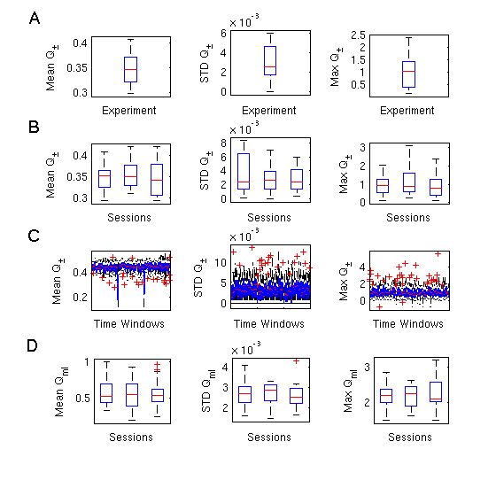
Figure 2: Properties of the static and dynamic modularity indices $Q_{\pm}$ and $Q_{ml}$. The mean (column 1), standard deviation (column 2), and maximum (column 3) of the static modularity index $Q_{\pm}$ is shown for (A) the large scale (entire experiment), (B) the mesoscopic scale (three experimental sessions), and (C) the small scale (individual time windows) over the $100$ samplings. Row (D) shows the mean (column 1), standard deviation (column 2), and maximum (column 3) of the dynamic modularity index $Q_{ml}$ over the $100$ samplings. In the figure, the standard deviation is abbreviated as STD. Boxplots indicate 95% confidence intervals over subjects.

We used one-sample $t$-tests to test statistically whether the differences between representative values from the real networks and null model networks over the subject population was significantly different from zero. The results, which we reported in the main manuscript, indicated that in contrast to what we observed using each of the three null models, the human brain displayed a heightened modular structure. That is, it is composed of more modules, which have smaller sizes. Considering the three null models in order, this suggests that cortical connectivity has a precise topological organization, that cortical regions consistently maintain individual connectivity signatures necessary for cohesive community organization, and that functional communities evolve cohesively in time (see Figure 2 in the main manuscript). Importantly, the stationarity of modular organization $\zeta$ was also higher in the human brain than in the connectional or nodal null models, indicating a cohesive temporal evolution of functional communities.

Temporal Dynamics of Brain Architecture and Learning

In the present study, we have attempted to determine whether changes in the dynamic modular architecture of functional connectivity is shaped by learning. We assessed the learning in each session using the slope of the movement times (MT) of that session. Movement time is defined as the difference between the time of the first button press and the time of the last button press in a single sequence (see Figure S1B). During successful learning, movement time is known to fall logarithmically with time[1]. However, two subjects from session 1 and one subject from session 2 showed an increasing movement time as the session progressed. We therefore excluded these three data points in subsequent comparisons due to the decreased likelihood that successful learning was taking place. This process of screening participants based on movement time slope is consistent with previous work suggesting that fMRI activation patterns during successful performance might be inherently different when performance is unsuccessful [53].

In principle, modular architecture might vary with learning by displaying changes in global diagnostics such as the number of modules or the modularity index $Q$ or by displaying more specific changes in the composition of modules. To measure changes in the composition of modules, we defined the flexibility of a node $f_{i}$ to be the number of times that node changed modular assignment throughout the session, normalized by the total number of changes that were possible (i.e., by the number of consecutive pairs of layers in the multilayer framework). We then defined the flexibility of the entire network as the mean flexibility over all nodes in the network: $F=\frac{1}{N}\sum_{i=1}^{N}f_{i}$.

Statistics and Software

We implemented all computational and simple statistical operations using the software packages MATLAB^® (2007a, The MathWorks Inc., Natick, MA) and Statistica^® (version 9, StatSoft Inc.). We performed the network calculations using a combination of in-house software (including multilayer community detection code [43]) and the Brain Connectivity Toolbox [40].

Supplementary Results

Degeneracies of $Q$

As discussed earlier in the Methods section, we focused in this investigation on the mean properties of ensembles of partitions rather than on detailed properties of individual partitions. Our approach was motivated by recent work indicating that the optimization of modularity and similar quality functions is hampered by the complicated shape of the optimization landscape, which includes a large number of partitions with near-optimum values that collectively form a high modularity plateau [35]. To quantify and address this degeneracy of $Q_{\pm}$ and $Q_{ml}$, we now provide supplementary results on the mean, standard deviation, and maximum values of $Q_{\pm}$ and $Q_{ml}$ over the $100$ samples of the plateau computed for all real networks in both the static and dynamic frameworks.

The mean number of modules in a given partition in the static framework was $\bar{n}\approx 3.08$ for the entire experiment, $\bar{n}\approx 3.07$ for individual experimental sessions, and $\bar{n}\approx 3.55$ for the small intra-session time windows. The mean number of modules in a given partition in the multilayer framework was $\bar{n}\approx 6.00$. We have therefore chosen to sample the quality functions $Q_{\pm}$ and $Q_{ml}$ a total of $100$ times (which is more than $2^{\bar{n}-1}$ in each case, and therefore adequately samples the degenerate near-optimum values of $Q_{\pm}$ and $Q_{ml}$ [35]). In order to characterize the distribution of solutions found in these $100$ samplings, we have computed the mean, standard deviation, and maximum of $Q_{\pm}$ (static cases) and $Q_{ml}$ (dynamic cases); see Figure S2. We found that the values of $Q_{\pm}$ and $Q_{ml}$ are tightly distributed, and that the maximum values of $Q_{\pm}$ or $Q_{ml}$ are between $0$ and $3$ standard deviations higher than the mean. Although we remain cautious because we have not explored all possible computational heuristics, we are nevertheless encouraged by these results that the mean values of $Q_{\pm}$ and $Q_{ml}$ that we have reported are representative of the true maximization of the two quality functions.

Reproducibility

We calculated the intra-class correlation coefficient (ICC), to determine whether values of $Q_{\pm}$ and $Q_{ml}$ derived from a single individual over the $100$ samples were more similar than values of $Q_{\pm}$ or $Q_{ml}$ derived from different individuals. The ICC is a measure of the total variance for which between-subject variation accounts [54, 55], and it is defined as

$$\mathrm{ICC}=\frac{\sigma^{2}_{bs}}{\sigma^{2}_{bs}+\sigma^{2}_{ws}}\,,$$ (7)

where $\sigma_{bs}$ is the between-subject variance and $\sigma_{ws}$ is the pooled within-subject variance (‘pooled’ indicates that variance was estimated for each subject and then averaged over subjects). The ICC is normalized to have a maximum value of $1$; values above $0.5$ indicate that there is more variability between $Q_{\pm}$ and $Q_{ml}$ values from different subjects than between $Q_{\pm}$ and $Q_{ml}$ values from the same subject. In the static framework, the ICC was $0.9884$ at the large scale (the entire experiment), an average of $0.9863$ at the intermediate scale (three experimental sessions), and an average of $0.9847$ at the small scale (individual time windows). In the multilayer framework, we calculated that ICC $\approx 0.9983$. These results collectively indicate that the $Q_{\pm}$ and $Q_{ml}$ values that we reported in this work were significantly reproducible over the $100$ samples of the respective quality function landscape. That is, the $Q_{\pm}$ or $Q_{ml}$ values drawn from the $100$ samples of a single subject’s network modularity landscape were more similar than $Q_{\pm}$ or $Q_{ml}$ values drawn from different subjects.

Effect of the Inter-Layer Coupling Parameter

The multilayer network framework requires one to define a coupling parameter $C$ that indicates the strength of the connections from a node in one time window to itself in the two neighboring time windows [43]. In order to be sensitive to both temporal dynamics and intra-layer network architecture, the coupling parameter should be on the same scale of values as the edge weights. For example, if edge weights are coherence values lying between $0$ and $1$, then the coupling parameter also ought to lie between $0$ and $1$. In the results that we presented in the main manuscript, we set the coupling parameter to be $C=1$, which is the highest value consistent with the intra-layer edge weights given by the normalized coherence. However, if we were to alter the coupling value, one might expect the number of communities to be altered in kind. As the strength of the coupling is increased, one might expect fewer communities to be uncovered due to the increased temporal dependence between layers [43]. Similarly, as the inter-layer coupling is weakened, one might expect more communities to be detected.

To probe the effect of the inter-layer coupling strength, we thus varied $C$ from well below to well above the maximum intra-layer edge weight ($0.2\leq C\leq 2$). In Figure S3 (cortical network results are shown in blue), we illustrate the effects of sweeping over this coupling parameter on our four diagnostics. The modularity index $Q_{ml}$ increases with increasing inter-layer coupling, whereas the other three diagnostics—number of modules, module size, and stationarity—increase initially and then plateau approximately at about $C=1$ and above. The change in behavior near $C=1$ can be rationalized as follows: For $C<1$, intra-layer edge weights dominate the modularity optimization, whereas inter-layer edge weights dominate for $C>1$. The proposed choice of $C=1$ therefore balances the impact of known coherence in brain activity (as given by the intra-layer edge weights) on measured architectural adaptations and is therefore a natural choice with which to investigate biologically meaningful organization.

We also computed $100$ temporal, nodal, and connectional null model networks for each of the additional coupling parameter values (see Figure S3; null model network results shown in green, orange, and red). The results indicate that the relationship between diagnostics in the cortical networks and null model networks is dependent on the diagnostic. For example, modularity values of null model networks are consistently lower than modularity values of cortical networks. However, stationarity in the null model networks is lower than that in cortical networks for small values of $C$ but higher than that of cortical networks for high values of $C$. This nontrivial behavior suggests an added sensitivity of the proposed null model networks to the multilayer network construction, which might be useful in other experimental contexts and therefore warrants further investigation.

Effect of the Time Window Length

In the construction of networks at the smallest time scale, it is necessary to choose a length of the time window $T$. In choosing this time window length, two considerations are important: (1) the time window must be short enough to adequately measure temporal evolution of network structure, and (2) the time window must be long enough to adequately estimate the functional association between two time series using (for example) the correlation or coherence [56]. In the main text, we reported results for time windows of 80 data points in length. This gives 25 time windows in each experimental session, for a total of 75 time windows over the 3 sessions. In addition to this extensive coverage of the underlying temporal dynamics, the choice of a time window of 80 data points in length also ensures that 20 data points can be used for the estimation of the functional association between time series in the frequency band of interest—i.e., at wavelet scale two (0.06–0.12 Hz). If one were to increase the time window length, one would expect a decreased ability to measure temporal variations due to the presence of fewer time windows per session. If one were to decrease the time window length, one would expect increased variance in the estimation of the functional association between time series due to the use of fewer data points in the estimation of either the coherence or the correlation [16].

To probe the effect of the time window length, we varied $T$ from $T=80$ to $T=110$ (see Figure S4; cortical network results are shown in blue). We find that the stationarity of the modules increases with increasing time window length. As $T$ is increased, the functional association between any two nodes is averaged over a longer time series, so small adaptations over shorter time scales can no longer be measured. This smoothing is likely the cause of the increased stationarity that we find at high values of $T$. It suggests that functional association measured over long time windows is less dependent on the time window being used than functional association measured over short time windows. This finding supports our choice of short time windows in order to measure dynamic adaptations in network architecture.

We also computed $100$ temporal, nodal, and connectional null model networks for each of the additional time window lengths (see Figure S4; null model network results are shown in green, orange, and red). The results indicate that the relationships between diagnostics in the cortical networks and null model networks are largely conserved across time window lengths.

Learning and Flexibility

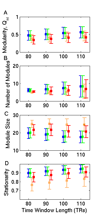
Figure 4: Effect of the time window length $T$ on the four diagnostics in this study: modularity index $Q_{ml}$, number of modules $n$, module size (i.e., number of nodes) $s$, and module stationarity $\zeta$. We first averaged values over 100 ‘optimal’ partitions (see the discussion in the text), so this figure gives mean values of all diagnostics. The error bars indicate standard deviations over subjects and sessions. In the figure, we give time windows in terms of the number of data points in the time series (i.e., the number of TRs). Colors indicate network type: cortical network (blue), temporal null model network (green), nodal null model network (orange), and connectional null model network (red). Error bars for different network types at a given value of $T$ (80, 90, 100, 110) are offset from each other for better visualization.

In the main text, we reported a significant correlation between the flexibility of dynamic modular architecture in a given experimental session, as measured by the (normalized) number of times a node changes module allegiance, and learning in the subsequent experimental sessions, as measured by the slope of the movement time (see Methods). We found that the mean value of flexibility was approximately $0.30$, that it fluctuated over the three experimental sessions, and that the values were highest in the second experimental session (see Table 2 in this Supplement). We followed this large-scale calculation with an investigation into the relationship between nodal flexibility (in particular brain regions) and learning. We found, as shown Figure 4 of the main manuscript, that the flexibility of a large number of brain regions could be used to predict learning in the following session. Here we also note that these regions were not those with highest flexibility or lowest flexibility in the brain. In fact, the flexibility of those regions that predicted learning was not significantly different from the flexibility of those regions that did not predict learning: $t\approx 0.01$ $p\approx 0.98$ (Session 1) and $t\approx 0.87$, $p\approx 0.38$ (Session 2).

In addition to those results reported in the main manuscript, we tested whether the flexibility of the cortical networks was significantly different from the flexibility expected in the (connectional, nodel, and temporal) random network null models. As we show in Table 3 in this Supplement, the flexibility of the connectional and nodal null model networks was significantly higher than that of the cortical networks, and we found no discernible differences between the cortical networks and the temporal null model networks. We found the greatest degree of flexibility in the nodal null model, in which individual nodes in any given time window were coupled to randomly selected nodes in the following time window. It is thus plausible that the subsequent disruption of nodal identity caused nodes to change computed module allegiances in this null model.

Robustness to Alternative Definitions

It is important to assess the robustness of our findings to different definitions of flexibility. We therefore defined an alternative flexibility measure $f^{\prime}_{i}$ to be the number of communities (modules) to which a node belongs at some point in a given experimental session. The mean alternative flexibility $F^{\prime}$ is then given by averaging $f^{\prime}_{i}$ over all nodes in the network: $F^{\prime}=\frac{1}{N}\sum_{i=1}^{N}f^{\prime}_{i}$. Using this alternative definition of flexibility, we again tested for differences between the cortical network and the three random network null models. As shown in Tables 2 and 3, the $F^{\prime}$ values of cortical networks were also significantly different from those in the null model networks. Interestingly, for this alternative definition, the temporal network null model exhibits significantly lower flexibility than the cortical networks, suggesting that this measure of flexibility might be sensitive to biologically relevant temporal evolution of modular architecture. Finally, we tested whether this alternative definition of flexibility also displayed a relationship to learning. Flexibility and learning were not significantly correlated in Session 1 ($r\approx 0.02$, $p\approx 0.90$) or in Session 2 ($r\approx 0.18$, $p\approx 0.48$), but flexibility in Session 1 was predictive of learning in Session 2 ($r\approx 0.64$, $p\approx 0.002$), and flexibility in Session 2 was predictive of learning in Session 3 ($r\approx 0.51$, $p\approx 0.019$). These results for the alternative flexibility $F^{\prime}$ are consistent with those of the original definition $F$, suggesting that our findings are robust.

Supplementary Discussion

Resolution Limit of Modularity

When detecting communities by optimizing modularity and similar quality functions, it is important to note that modularity suffers from a resolution limit [57, 34, 33, 35]. As a result, the maximum-modularity partition can be biased towards a particular module size and can have difficulty resolving modules smaller than that size. Consequently, small modules of potential interest have the potential to be hidden within larger groups of nodes that have been detected. Modularity’s resolution limit is particularly prevalent in sparse networks, binary networks, and large networks, and its effects tend to be much less significant in networks of the type (dense, weighted, and small) that we have studied [35].

Measuring Differences in Brain States

In the present work, we have characterized differences in brain states during learning by examining the global network architecture and measuring differences between that architecture over three experimental sessions. An alternative line of investigation would be to seek network motifs (i.e., small patterns of nodes and edges) that have the potential to distinguish between brain states. This could be done using statistical methods [58], machine-learning techniques [59], or a combination of the two [60]. Our approach, however, has the advantage of assessing alterations in large-scale achitectural properties rather than differences in small parts of that architecture. Additionally, the approach that we have chosen provides a direct characterization of the underlying functional connectivity architecture irrespective of differences between brain states. Using this approach, we have therefore been able to demonstrate, for example, that there is significant non-random modular organization across multiple temporal scales.

A Note on Computational Time

The investigations that we reported in the present work involved about $10,000$ CPU-days, and our study was therefore made possible by the use of two computing clusters available at the Institute for Collaborative Biotechnologies at UC Santa Barbara. Cluster 1 was composed of 42 Dell SC1425s (dual single-core Xeon 2.8GHz, 4GB memory), 5 Dell PE1950s (dual quad-core Xeon E5335 2.0GHz, 8GB memory), 1 Dell 2850 (RAID storage includes 500GB for the home directory), and MATLAB^® MDCE with 128 worker licenses (cluster currently has 124 compute cores), Gigabit Ethernet, Software RAID backup node (converted compute node) with 673GB software RAID backup. Cluster 2 was composed of 20 HP Proliant DL160 G6s (dual quad-core E5540 “Nehalem” 2.53GHz, 24GB memory), 1 HP DL180 G6 (RAID storage includes 2.1TB for the home directory), MATLAB^® MDCE with 160 worker licenses (cluster currently has 160 compute cores), Gigabit Ethernet, and a storage node with 4.6TB of RAID storage (for backup).

We performed maximization of the quality functions ($Q_{pm}$, $Q_{ml}$) a total of $100$ times for every connectivity matrix under study. In the static connectivity investigation, we constructed connectivity matrices for 20 subjects, 3 temporal scales (encompassing 1 experiment, 3 experimental sessions, and 25 time windows), and 1 random network null model. In the dynamic connectivity investigation, we constructed connectivity matrices for 20 subjects, 18–34 time windows, 3 different null models, 10 values of the inter-layer coupling $C$, and 4 values of time window length (80, 90, 100, and 110 TRs). In light of the computational extent of this work, we note that we did not employ Kernighan-Lin (KL) node-swapping steps [61] in our optimization of $Q_{pm}$ or $Q_{ml}$, as they would be computationally prohibitive and are not necessary in the present context. KL steps move individual nodes between communities in order to further optimize a single sample of $Q_{pm}$ or $Q_{ml}$ [62, 63, 33]. As we focus on the mean properties of ensembles of partitions (and use them to report reliable measurements of architectural properties) rather than on the values of diagnostics for any individual partitions, KL steps that provide a marginal increase in the value of $Q_{pm}$ or $Q_{ml}$ would not be helpful for our study.

Frontal pole	Cingulate gyrus, anterior
Insular cortex	Cingulate gyrus, posterior
Superior frontal gyrus	Precuneus cortex
Middle frontal gyrus	Cuneus cortex
Inferior frontal gyrus, pars triangularis	Orbital frontal cortex
Inferior frontal gyrus, pars opercularis	Parahippocampal gyrus, anterior
Precentral gyrus	Parahippocampal gyrus, posterior
Temporal pole	Lingual gyrus
Superior temporal gyrus, anterior	Temporal fusiform cortex, anterior
Superior temporal gyrus, posterior	Temporal fusiform cortex, posterior
Middle temporal gyrus, anterior	Temporal occipital fusiform cortex
Middle temporal gyrus, posterior	Occipital fusiform gyrus
Middle temporal gyrus, temporooccipital	Frontal operculum cortex
Inferior temporal gyrus, anterior	Central opercular cortex
Inferior temporal gyrus, posterior	Parietal operculum cortex
Inferior temporal gyrus, temporooccipital	Planum polare
Postcentral gyrus	Heschl’s gyrus
Superior parietal lobule	Planum temporale
Supramarginal gyrus, anterior	Supercalcarine cortex
Supramarginal gyrus, posterior	Occipital pole
Angular gyrus	Caudate
Lateral occipital cortex, superior	Putamen
Lateral occipital cortex, inferior	Globus pallidus
Intracalcarine cortex	Thalamus
Frontal medial cortex	Nucleus Accumbens
Supplemental motor area	Parahippocampal gyrus (superior to ROIs 34,35)
Subcallosal cortex	Hippocampus
Paracingulate gyrus	Brainstem

Table 1: Brain regions present in the Harvard-Oxford Cortical and Subcortical Parcellation Scheme provided by FSL [2, 9].

Type of Flexibility	Session	Cortical	Connectional	Nodal	Temporal
$F$
	1	0.027$\pm$0.009	0.041$\pm$0.008	0.070$\pm$0.001	0.027$\pm$0.010
	2	0.030$\pm$0.009	0.042$\pm$0.007	0.067$\pm$0.001	0.030$\pm$0.009
	3	0.027$\pm$0.008	0.039$\pm$0.008	0.064$\pm$0.001	0.026$\pm$0.009
$F^{\prime}$
	1	1.93$\pm$0.30	2.58$\pm$0.25	3.19$\pm$0.01	1.90$\pm$0.31
	2	1.95$\pm$0.27	2.53$\pm$0.23	3.01$\pm$0.01	1.94$\pm$0.28
	3	1.86$\pm$0.25	2.43$\pm$0.23	2.92$\pm$0.01	1.85$\pm$0.26

Table 2: Flexibility in cortical network and random network null models for two different definitions of flexibility. One definition is $F=\frac{1}{N}\sum_{i=1}^{N}f_{i}$, where $f_{i}$ is the number of times node $i$ changes module allegiance in a given experimental session divided by the total number of possible changes (i.e., by the number of consecutive pairs of layers in the multilayer framework). The second definition is $F^{\prime}=\frac{1}{N}\sum_{i=1}^{N}f^{\prime}_{i}$, where $f^{\prime}_{i}$ is defined as the total number of modules of which node $i$ is a member at some point in the experiment session. We also indicate mean values and standard deviations.

Type of Flexibility	Session	Null Model	$t$-statistic	$p$-value
$F$	1	Connectional	$-10.62$	$1.2\times 10^{-18}$
		Nodal	$-47.56$	$1.1\times 10^{-75}$
		Temporal	$-0.64$	0.51
	2	Connectional	$-9.47$	$5.5\times 10^{-16}$
		Nodal	$-43.41$	$1.7\times 10^{-71}$
		Temporal	$-0.16$	0.86
	3	Connectional	$-9.86$	$1.1\times 10^{-16}$
		Nodal	$-46.95$	$4.5\times 10^{-75}$
		Temporal	0.77	0.43
$F^{\prime}$	1	Connectional	$-14.54$	$1.8\times 10^{-27}$
		Nodal	$-43.44$	$1.6\times 10^{-71}$
		Temporal	4.67	$8.4\times 10^{-6}$
	2	Connectional	$-14.04$	$2.3\times 10^{-26}$
		Nodal	$-39.67$	$2.1\times 10^{-67}$
		Temporal	3.95	$1.3\times 10^{-4}$
	3	Connectional	$-14.87$	$3.5\times 10^{-28}$
		Nodal	$-43.80$	$6.9\times 10^{-72}$
		Temporal	2.79	0.0061

Table 3: Results for one-sample $t$-tests on flexibility in cortical networks versus random network null models for two different definitions of flexibility ($F$ and $F^{\prime}$). We report these results for the connectional, nodal, and temporal null models. Negative $t$-statistics indicate that the flexibility of the null model network is greater than that of the cortical network, and positive $t$-statistics indicate that the flexibility of the cortical network is greater than that of the null model network.

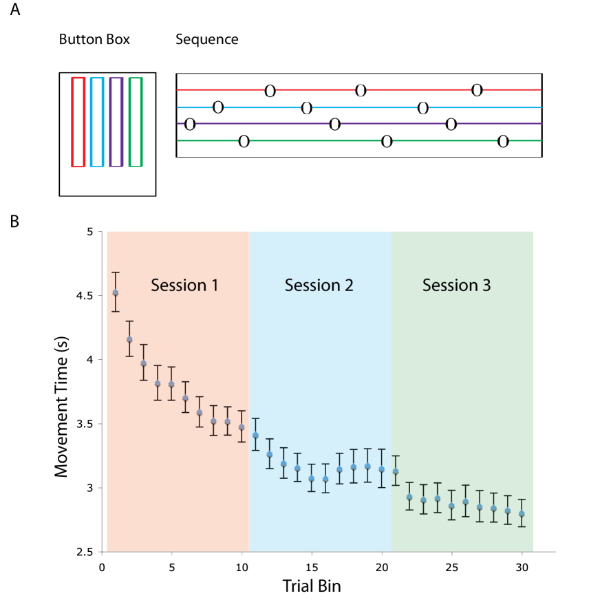
Figure 1: Experimental Setup and Learning (A) Schematic of the cued sequence production (CSP) task. The response or “button” box (left) had four response buttons that were color-coded to match the notes on the “musical staff” (right) presented to the subject in the visual stimulus. This visual stimulus was composed of 12 notes in sequence. Here we show one example of a single sequence. (B) Movement time as a function of practiced trials, whose decreasing slope indicates that learning is occuring. (We have aggregated trials into 10 trial bins per session.)

Addendum

This work was supported by the David and Lucile Packard Foundation, PHS Grant NS44393, the Institute for Collaborative Biotechnologies through contract no. W911NF-09-D-0001 from the U.S. Army Research Office, and the NSF (DMS-0645369). M.A.P. acknowledges a research award (#220020177) from the James S. McDonnell Foundation.
We thank Aaron Clauset for useful discussions and John Bushnell for technical support.
Competing Interests: The authors declare that they have no competing financial interests.
Correspondence: Correspondence and requests for materials should be addressed to D.S.B. (email: dbassett@physics.ucsb.edu).

References

- [1] Snoddy, G. S. Learning and stability: A psychophysical analysis of a case of motor learning with clinical applications. Journal of Applied Psychology 10, 1–36 (1926).
- [2] Smith, S. M. et al. Advances in functional and structural MR image analysis and implementation as FSL. Neuroimage 23, 208–219 (2004).
- [3] Bassett, D. S. & Bullmore, E. T. Small-world brain networks. Neuroscientist 12, 512–523 (2006).
- [4] Bassett, D. S. & Bullmore, E. T. Human brain networks in health and disease. Curr Opin Neurol 22, 340–347 (2009).
- [5] Bullmore, E. & Sporns, O. Complex brain networks: Graph theoretical analysis of structural and functional systems. Nat Rev Neurosci 10, 186–198 (2009).
- [6] Wang, J. et al. Parcellation-dependent small-world brain functional networks: A resting-state fMRI study. Hum Brain Mapp 30, 1511–1523 (2009).
- [7] Zalesky, A. et al. Whole-brain anatomical networks: Does the choice of nodes matter? Neuroimage 50, 970–983 (2010).
- [8] Bassett, D. S., Brown, J. A., Deshpande, V., Carlson, J. M. & Grafton, S. T. Conserved and variable architecture of human white matter connectivity. Neuroimage 54, 1262–79 (2011).
- [9] Woolrich, M. W. et al. Bayesian analysis of neuroimaging data in FSL. Neuroimage 45, S173–S186 (2009).
- [10] Bullmore, E. et al. Wavelets and statistical analysis of functional magnetic resonance images of the human brain. Stat Methods Med Res 12, 375–399 (2003).
- [11] Bullmore, E. et al. Wavelets and functional magnetic resonance imaging of the human brain. Neuroimage 23, S234–S249 (2004).
- [12] Brammer, M. J. Multidimensional wavelet analysis of functional magnetic resonance images. Hum Brain Mapp 6, 378–382 (1998).
- [13] Achard, S., Salvador, R., Whitcher, B., Suckling, J. & Bullmore, E. A resilient, low-frequency, small-world human brain functional network with highly connected association cortical hubs. J Neurosci 26, 63–72 (2006).
- [14] Bassett, D. S., Meyer-Lindenberg, A., Achard, S., Duke, T. & Bullmore, E. Adaptive reconfiguration of fractal small-world human brain functional networks. Proc Natl Acad Sci USA 103, 19518–19523 (2006).
- [15] Achard, S. & Bullmore, E. Efficiency and cost of economical brain functional networks. PLoS Comput Biol 3, e17 (2007).
- [16] Achard, S., Bassett, D. S., Meyer-Lindenberg, A. & Bullmore, E. Fractal connectivity of long-memory networks. Phys Rev E 77, 036104 (2008).
- [17] Bassett, D. S., Meyer-Lindenberg, A., Weinberger, D. R., Coppola, R. & Bullmore, E. Cognitive fitness of cost-efficient brain functional networks. Proc Natl Acad Sci USA 106, 11747–11752 (2009).
- [18] Lynall, M. E. et al. Functional connectivity and brain networks in schizophrenia. J Neurosci 30, 9477–87 (2010).
- [19] Percival, D. B. & Walden, A. T. Wavelet Methods for Time Series Analysis (Cambridge University Press, 2000).
- [20] Sun, F. T., Miller, L. M. & D’Esposito, M. Measuring interregional functional connectivity using coherence and partial coherence analyses of fMRI data. Neuroimage 21, 647–658 (2004).
- [21] Barnes, A., Bullmore, E. T. & Suckling, J. Endogenous human brain dynamics recover slowly following cognitive effort. PLoS One 4, e6626 (2009).
- [22] Lowe, M. J., Mock, B. J. & Sorenson, J. A. Functional connectivity in single and multislice echoplanar imaging using resting state fluctuations. Neuroimage 7, 119–132 (1998).
- [23] Cordes, D. et al. Mapping functionally related regions of brain with functional connectivity MR imaging. Am J Neuroradiol 21, 1636–1644 (2000).
- [24] Cordes, D. et al. Frequencies contributing to functional connectivity in the cerebral cortex in “resting-state” data. Am J Neuroradiol 22, 1326–1333 (2001).
- [25] Fair, D. A. et al. A method for using blocked and event-related fMRI data to study ‘resting state’ functional connectivity. Neuroimage 35, 396–405 (2007).
- [26] Meunier, D., Achard, S., Morcom, A. & Bullmore, E. Age-related changes in modular organization of human brain functional networks. Neuroimage 44, 715–723 (2008).
- [27] Meunier, D., Lambiotte, R., Fornito, A., Ersche, K. D. & Bullmore, E. T. Hierarchical modularity in human brain functional networks. Front Neuroinformatics 3, 37 (2009).
- [28] Rahman, N. A. A Course in Theoretical Statistics (Charles Griffin and Company, 1968).
- [29] He, Y., Chen, Z. J. & Evans, A. C. Small-world anatomical networks in the human brain revealed by cortical thickness from MRI. Cereb Cortex 17, 2407–2419 (2007).
- [30] Benjamini, Y. & Yekutieli, Y. The control of the false discovery rate in multiple testing under dependency. Ann Stat 29, 1165–1188 (2001).
- [31] Genovese, C. R., Lazar, N. A. & Nichols, T. E. Thresholding of statistical maps in functional neuroimaging using the false discovery rate. Neuroimage 15, 870–878 (2002).
- [32] Newman, M. E. J. Networks: An Introduction (Oxford University Press, 2010).
- [33] Porter, M. A., Onnela, J.-P. & Mucha, P. J. Communities in networks. Not Amer Math Soc 56, 1082–1097, 1164–1166 (2009).
- [34] Fortunato, S. Community detection in graphs. Phys Rep 486, 75–174 (2010).
- [35] Good, B. H., de Montjoye, Y. A. & Clauset, A. Performance of modularity maximization in practical contexts. Phys Rev E 81, 046106 (2010).
- [36] Girvan, M. & Newman, M. E. Community structure in social and biological networks. Proc Natl Acad Sci U S A 99, 7821–6 (2002).
- [37] Girvan, M. & Newman, M. E. Community structure in social and biological networks. Proc Natl Acad Sci USA 99, 7821–6 (2002).
- [38] Brandes, U. et al. On modularity clustering. IEEE Transactions on Knowledge and Data Engineering 20, 172–188 (2008).
- [39] Chen, Z. J., He, Y., Rosa-Neto, P., Germann, J. & Evans, A. C. Revealing modular architecture of human brain structural networks by using cortical thickness from MRI. Cerebral Cortex 18, 2374–2381 (2008).
- [40] Rubinov, M. & Sporns, O. Complex network measures of brain connectivity: Uses and interpretations. Neuroimage 52, 1059–1069 (2009).
- [41] Blondel, V. D., Guillaume, J. L., Lambiotte, R. & Lefebvre, E. Fast unfolding of community hierarchies in large networks. J Stat Mech P10008 (2008).
- [42] Traag, V. A. & Bruggeman, J. Community detection in networks with positive and negative links. Phys Rev E 80, 036115 (2009).
- [43] Mucha, P. J., Richardson, T., Macon, K., Porter, M. A. & Onnela, J.-P. Community structure in time-dependent, multiscale, and multiplex networks. Science 328, 876–878 (2010).
- [44] Bassett, D. S. et al. Efficient physical embedding of topologically complex information processing networks in brains and computer circuits. PLoS Comput Biol 6, e1000748 (2010).
- [45] Maslov, S. & Sneppen, K. Specificity and stability in topology of protein networks. Science 296, 910–913 (2002).
- [46] Molloy, M. & Reed, B. A critical point for random graphs with a given degree sequence. Random Structures and Algorithms 6, 161–180 (1995).
- [47] Traud, A. L., Frost, C., Mucha, P. J. & Porter, M. A. Visualization of communities in networks. Chaos 19, 041104 (2009).
- [48] Fruchtermann, T. M. J. & Reingold, E. M. Graph drawing by force-directed placement. Software, Practice and Experience 21, 1129–1164 (1991).
- [49] Kamada, T. & Kawai, S. An algorithm for drawing general undirected graphs. Information Processing Letters 31, 7–15 (1988).
- [50] Friston, K. J., Zarahn, E., Josephs, O., Henson, R. N. & Dale, A. M. Stochastic designs in event-related fMRI. Neuroimage 10, 607–619 (1999).
- [51] Benesty, J., Chen, J. & Huang, Y. Estimation of the coherence function with the MVDR approach. IEEE International Conference on Acoustic, Speech, and Signal Processing (2006).
- [52] Palla, G., Barabási, A. & Vicsek, T. Quantifying social group evolution. Nature 446, 664–667 (2007).
- [53] Callicott, J. H. et al. Physiological characteristics of capacity constraints in working memory as revealed by functional MRI. Cereb Cortex 9, 20–26 (1999).
- [54] Lachin, J. M. The role of measurement reliability in clinical trials. Clin Trials 1, 553–566 (2004).
- [55] McGraw, K. O. & Wong, S. P. Forming inferences about some intraclass correlation coefficients. Psychological Methods 1, 30–46 (1996).
- [56] Fenn, D. J. et al. Dynamic communities in multichannel data: an application to the foreign exchange market during the 2007-2008 credit crisis. Chaos 19, 033119 (2009).
- [57] Fortunato, S. & Barthélemy, M. Resolution limit in community detection. Proc Natl Acad Sci USA 104, 36–41 (2007).
- [58] Zalesky, A., Fornito, A. & Bullmore, E. T. Network-based statistic: Identifying differences in brain networks. Neuroimage 53, 1197–207 (2010).
- [59] Richiardi, J., Eryilmaz, H., Schwartz, S., Vuilleumier, P. & Van De Ville, D. Decoding brain states from fMRI connectivity graphs. Neuroimage doi:10.1016/j.neuroimage.2010.05.081 (2010).
- [60] Shinkareva, S. V., Gudkov, V. & Wang, J. A network analysis approach to fMRI condition-specific functional connectivity. arXiv:1008.0590 (2010).
- [61] Kernighan, B. W. & Lin, S. An efficient heuristic procedure for partitioning graphs. The Bell System Technical Journal 49, 291–307 (1970).
- [62] Richardson, T., Mucha, P. J. & Porter, M. A. Spectral tripartitioning of networks. Physical Review E 80, 036111 (2009).
- [63] Newman, M. E. J. Finding community structure in networks using the eigenvectors of matrices. Physical Review E 74, 036104 (2006).