The longest timescale X-ray variability reveals an evidence for active galactic nuclei in the high accretion state

Abstract

The All Sky Monitor (ASM) onboard the Rossi X-ray Timing Explorer (RXTE) has continuously monitored a number of Active galactic nuclei (AGNs) with similar sampling rates for 14 years from 1996 January to 2009 December. Utilizing the archival ASM data of 27 AGNs, we calculate the normalized excess variances of the 300-day binned X-ray light curves on the longest timescale (between 300 days and $14$ years) explored so far. The observed variance appears to be independent of AGN black hole mass and bolometric luminosity, respectively. According to the scaling relation with black hole mass (and bolometric luminosity) from Galactic black hole X-ray binaries (GBHs) to AGNs, the break timescales which correspond to the break frequencies detected in the power spectral density (PSD) of our AGNs are larger than binsize (300 days) of the ASM light curves. As a result, the singly-broken power-law (soft-state) PSD predicts the variance to be independent of mass and luminosity, respectively. Nevertheless, the doubly-broken power-law (hard-state) PSD predicts, with the widely accepted ratio of the two break frequencies, that the variance increases with increasing mass and decreases with increasing luminosity, respectively. Therefore, the independence of the observed variance on mass and luminosity suggests that AGNs should have the soft-state PSDs. If taking into account the scaling of breaking timescale with mass and luminosity synchronously, the observed variances are also more consistent with the soft-state than the hard-state PSD predictions. With the averaged variance of AGNs and the soft-state PSD assumption, we obtain a universal PSD amplitude of $0.030\pm 0.022$. By analogy with the GBH PSDs in the high/soft state, the longest timescale variability supports the standpoint that AGNs are scaled-up GBHs in the high accretion state, as already implied by the direct PSD analysis.

1 Introduction

Active galactic nuclei (AGNs) might be scaled-up Galactic black hole X-ray binaries (GBHs) (e.g., McHardy et al. 2006) since both are powered by similar physical process, i.e., accretion onto (super-massive and stellar-mass, respectively) black hole. Therefore, it is important and fundamental to explore the observational similarities between the two classes of black hole accreting system on very different scales. Because it originates in the region mostly close to the black hole, the X-ray emission carries the most pivotal messages for the black hole accretion process. Both AGNs and GBHs exhibit strong X-ray variability, which is usually quantified by the power spectral density (PSD; $P_{\nu}\propto\nu^{\alpha}$) of their X-ray light curves.

The GBH PSDs between 0.001 and 100 Hz are closely related to their X-ray spectral states (e.g., Done & Gierliński 2005; Klein-Wolt & van der Klis 2008). A template source mostly quoted is the persistent source, Cyg X-1. In its low/hard state at which the energy spectrum is dominated by a strongly variable power-law component, the hard-state PSD of Cyg X-1 is approximately described by a doubly-broken power law (e.g., Pottschmidt et al. 2003), flattening from $\alpha\sim-2$ to $\alpha\sim-1$ at the (high-)frequency break ($\nu_{\rm b}\sim$ a few Hz) and further flattening to $\alpha\sim 0$ at the low-frequency break ($\nu_{\rm LFB}\sim$ a few tenth Hz) from high to low frequencies. The ratio of the two break frequencies is $\sim 10-100$. In its high/soft state, albeit the energy spectrum is dominated by a roughly constant thermal disc component, the highly variable power-law component is strong enough to construct the soft-state PSD of Cyg X-1, which is significantly distinguished from the hard-state PSD by showing only one (high-frequency) break ($\nu_{\rm b}\sim 15$ Hz). The soft-state PSD slope above and below $\nu_{\rm b}$ is $\alpha\sim-2$ and $\alpha\sim-1$, respectively, and the $-1$ slope can be extended down to many decades of frequencies without further flattening (e.g., Axelsson, Borgonovo, & Larsson 2006). However, as already shown by Pottschmidt et al. (2003), even in Cyg X-1, the GBH PSD shape is not as simple as usually assumed.

If the X-ray variability timescale linearly scales with black hole mass ($M_{\rm BH}$) from GBHs to AGNs, the state-transition timescales of a few days found in GBHs ($M_{\rm BH}\sim 10M_{\odot}$) suggest that AGNs of $M_{\rm BH}\sim 10^{7}M_{\odot}$ would show state transitions on timescales of a few thousand years. Thus, the state transitions of AGNs can not be verified by direct X-ray observations if AGNs do have state transitions behaving like GBHs and satisfy the generally accepted scaling law. Nevertheless, if we believe that AGNs have the same underlying variability mechanism as GBHs, the different sub-classes of AGNs might be reasonably assumed to correspond to different spectral states of GBHs. In fact, this assumption can be tested by comparing the PSDs of different types of AGNs with those of GBHs in different spectral states. However, the scaling of timescale with mass ascertain that it is very time-consuming to derive AGN PSDs. Compared to GBHs, the limited durations and low signal-to-noise ratios of AGN light curves usually produce incomplete and low quality PSDs. As a result, it is not easy to constrain PSD shapes and the important break frequencies for a large number of AGNs. Relatively high quality AGN PSDs obtained so far, actually available for a limited number (about a dozen) of Seyfert galaxies only, are almost analogous to GBH soft-state PSDs (e.g., Uttley & McHardy 2005). The PSDs of Seyfert galaxies show one break ($\nu_{\rm b}$) only, flattening from $\alpha\sim-2$ to $\alpha\sim-1$. With present data, the PSDs do not show further flattening down to the lowest frequencies ($\sim 10^{-8}$ Hz) which are $3-4$ decades lower than the break frequencies. Like GBHs in the high/soft state, the fact that Seyfert galaxies show the soft-state PSDs are strongly supported by their low radio fluxes and high accretion rates larger than two percent of the Edington accretion rate at which Cyg X-1 transits between the hard and soft spectral states (e.g., Maccarone et al. 2003).

Up to now, Ark 564 and NGC 3783 are the only AGNs whose PSD shows the second, low-frequency break ($\nu_{\rm LFB}$). Ark 564 has strong evidence for the second break in its PSD (Pounds et al. 2001; Papadakis et al. 2002; Markowitz et al. 2003; McHardy et al. 2007). Nevertheless, the very high (possibly super-Eddington) accretion rate ($\dot{\rm m}_{\rm E}\sim 1$, Romano et al. 2004) suggests that Ark 564 may resemble GBHs in the very high state rather than in the low/hard state (McHardy et al. 2007), since in the very high state GBH PSDs show two distinct breaks as well. The second break in the PSD of NGC 3783, firstly presented by Markowitz et al. (2003), was questioned by Summons et al. (2007) with the improved PSD. Moreover, the moderately high accretion rate ($\dot{\rm m}_{\rm E}\sim 0.07$, Uttley & McHardy 2005) and radio quietness (e.g., Reynolds 1997) suggest that NGC 3783 is analogous to GBHs in the high/soft state. Therefore, NGC 3783 also became one of AGNs showing soft-state PSD, which leaves Ark 564 as the only non-soft-state AGN.

The X-ray variability of AGNs can also be quantified with the normalized excess variance ($\sigma^{2}_{\rm NXS}$) of their X-ray light curves, which is approximately equal to the integral of the normalized PSDs of the same light curves (e.g., Vaughan et al. 2003; Zhang et al. 2005). Because it is much more easier to calculate the variances than to calculate the PSDs, the variances have been used to explore the scaling relation of the X-ray variability with black hole mass, i.e., the so-called variance-mass ($\sigma^{2}_{\rm NXS}-M_{\rm BH}$) relationship, and X-ray luminosity of AGNs. On timescale of about half day, the variance anti-correlates with mass (i.e., $\sigma^{2}_{\rm NXS}\propto M_{\rm BH}^{-1}$; e.g., Lu & Yu 2001; Bian & Zhao 2003; Liu & Zhang 2008; Zhou et al. 2010) and X-ray luminosity (e.g., Nandra et al. 1997). By scaling with Cyg X-1, the variance has been used as a method to estimate $M_{\rm BH}$ of AGNs (Nikolajuk et al. 2004; 2006; 2009; Gierliński et al. 2008; Zhang et al. 2005). Although the variance of an individual source does nothing for constraining AGN PSDs, the variance-mass relation, just requiring to calculate variances of a large sample of AGNs with known masses, has this function. If AGNs have the same underlying X-ray variability mechanism that scales with mass, the variance-mass relation can be reproduced from a universal AGN PSD model. The comparison between the observed and predicted variance-mass relation can determine AGN PSD shape and the scaling factors of its parameters with mass. For 10 Seyfert galaxies, which have been regularly observed in X-rays, the 2–10 keV variances calculated with 300-day long RXTE PCA light curves anti-correlate with masses, which can be fitted by the hard-state PSD model (Papadakis 2004). With ASCA light curves of about half-day long for a larger sample of AGNs, O’Neill et al. (2005) obtained a similar anti-correlation between variances and masses, which is also in agreement with the prediction of the hard-state PSD model. Using ${\it XMM-Newton}$ data on timescale of about half day, Papadakis et al. (2008b) and Miniutti et al. (2009) enlarged the AGN sample, especially objects with smaller masses, for the variance-mass relation. Papadakis et al. (2008a) also extended the study of the variance-mass relation to higher red-shift AGNs.

The studies of variance-mass relationship suggest that AGNs have the hard-state PSDs, which apparently is in contradiction with the conclusion that AGNs have the soft-state PSDs from the direct PSD analysis. Importantly, the AGN samples of Papadakis (2004) and O’Neill et al. (2005) include most of AGNs whose soft-state PSDs have been well determined. The reason for this inconsistency could be mainly due to the short duration of the light curves used to calculate the variances. In fact, even though AGNs do have the hard-state PSDs, the short timescale variances do not cover the frequencies where the low-frequency breaks locate for most of AGNs. On short timescales, the hard-state PSD predicts the same variance-mass relation as the soft-state PSD does. Short timescale variance-mass relation is thus not able to differentiate the two PSD models. Consequently, in order to demonstrate whether AGN PSDs have the second breaks, it is necessary to obtain variance-mass relation with very long timescale light curves, especially for AGNs with large masses. The values of $\nu_{\rm LFB}$ for the GBH hard-state PSDs are about a few tenth of one Hz. If AGNs do show the hard-state PSDs, by scaling law of $\nu_{\rm LFB}$ with mass, $\nu_{\rm LFB}$ would be $\sim 10^{-7}$ Hz (on the order of one year) for AGNs with $M_{\rm BH}\sim 10^{7}M_{\odot}$. Therefore, in order to effectively distinguish the two AGN PSD models with variance-mass relation, a large number of AGNs should be continuously monitored for tens of years.

The longest data stream with roughly continuous and regular sampling mode are from the ASM onboard RXTE. The ASM has been monitoring a large number of AGNs since January 1996. In this paper, we will use the ASM data to obtain the variances of 27 AGNs on the longest timescale so far, with which we are in an attempt to differentiate the two AGN PSD models.

2 The ASM Data and AGN Sample

The ASM operates in the 1.5 to 12 keV energy band and scans most of the sky every 1.5 hours. We start our analysis with the data of the one-day averages from the ASM quick-look pages. Each one-day averaged data is the average of the fitted source fluxes from a number (typically 5 to 10) of individual 90 second dwells over that day, and is quoted as the nominal 2–10 keV ASM count rate (counts per second). We make use of the full ASM data stream from 1996 January 1 to 2009 December 31 (Modified Julian Day [MJD] $50083-55196$), which provides 14-year long X-ray light curves for a large number of AGNs. In the ASM quick-look pages, we select AGNs having a measurement of black hole mass in the literatures. Our final sample, tabulated in Table 1, contains 27 AGNs, including 20 broad-line Seyfert 1 (BLS1) and 7 narrow-line Seyfert 1 (NLS1) galaxies. Among them, we find bolometric luminosity of 20 AGNs and PSD break timescale ($1/\nu_{\rm b}$) of 12 AGNs in the literatures.

Due to low sensitivity, the ASM signal-noise ratios are quite low for AGNs. As two examples, the left plots of Figure 1 and Figure 2 show the background-subtracted one-day averaged ASM light curves for the lowest and highest count rate object Mrk 335 and IC 4329a among our AGN sample, respectively. It can been seen that the one-day averaged light curves contain many negative count rates. The light curves do not show legible variability trend either, mainly caused by strong Poisson noise. In order to acquire meaningful variability information of AGNs from the ASM data, it is necessary to rebin the one-day averaged light curves over very long timescale (e.g., 300 days as used in Section 4). The right plots of Figure 1 and Figure 2 present the 300-day averaged light curves of Mrk 335 and IC 4329a, showing that the two objects are indeed variable on such long timescale, though the errors are still large. For comparisons, the 300-day averaged light curves are also plotted on top of their respective one-day averaged light curves in the left plots of Figure 1 and Figure 2.

Onboard RXTE, the Proportional Counter Array (PCA) is much more sensitive than the ASM. To judge the quality of the ASM light curves, we compare the light curves obtained with PCA and ASM in the same time intervals. We choose two objects, namely IC 4329a and NGC 3227, to perform this comparison. The PCA monitored IC 4329a once every 4.26 days for a duration of 4.3 years, from 2003 April 8 to 2007 August 7 (MJD $52737-54319$; observation identifiers 80152-03, 80152-04, 90154-01, 91138-01, and 92108-01; see Markowitz 2009). NGC 3227 was monitored by the PCA with different observing schemes (see Uttley & McHardy 2005 for the details) for a duration of 7.4 years, from 1999 March 23 to 2006 August 13 (MJD $51260-53960$; observation identifiers 40151-01, 40151-08, 40151-09, 50153-07, 50153-08, 60133-05, 70142-01, 80154-01, 90160-04). We obtained the long-term PCA light curves of the two objects from HEASARC archive data search form, in which we selected ”XTE Target Index Catalog” and downloaded the merged light curves. We then re-selected the one-day averaged ASM light curves of the two objects in the same time intervals as spanned by their long term PCA light curves. Both the PCA and ASM light curves are averaged over 300 days, which are shown in Figure 3. In order to compare the PCA and ASM light curves easily, they are normalized to their respective mean count rates. Although the discrepancies of the normalized count rates between the ASM and PCA light curves are present in some points of the light curves and the PCA errors are much smaller than the ASM ones, the ASM light curves could still be thought to roughly track the PCA ones on binsize of 300 days. Therefore, the 300-day averaged ASM light curves can be used to study long-term variability of AGNs.

In the case of the heavily binned ASM light curves, the sampled PSD at $\nu_{\rm max}$ ($\nu_{\rm max}=1/(2\Delta t)$, where $\Delta t$ is the binsize of the light curves) might be massively affected by aliasing effects, specially because of $\nu_{\rm b}\gg\nu_{\rm min}$ ($\nu_{\rm min}=1/T$, where $T$ is the duration of the light curves) for most of objects. Therefore, the observed $\sigma^{2}_{\rm NXS}$ (see formula [1] for the definition) is not equal to the integral of the intrinsic PSD between $\nu_{\rm min}$ and $\nu_{\rm max}$. This should not be a serious problem, as it should affect all sources in a similar way. Nonetheless, it is worth investigating this aliasing effect by simulating a red-noise light curve. We follow the procedure described by Timmer & K$\ddot{\rm o}$nig (1995) to fake a light curve ( see Zhang 2002 and Zhang et al. 2004 for the details) by assuming a single power-law PSD ($P_{\nu}=a\times\nu^{\alpha}$, where $a$ is the PSD normalization factor). The experiment is performed twice, one with slope of $\alpha=-1$ and in the second case with $\alpha=-2$. In order to closely imitate the ASM light curves, we produce a light curve with 5100 points (one per day). For simplicity, we do not consider the effect of Poisson noise. The light curve is normalized to have a mean count rate of 0.2 and a variance of $7.56\times 10^{-2}$. The normalized variance is the integral of the intrinsic PSD between $1/T$ and $1/(2\Delta t)$, where $T=5100$ days and $\Delta t=1$ day correspond to the length and binsize of the simulated light curve. Under these assumptions, one can derive the value of $a$, which is $9.64\times 10^{-3}$ and $1.72\times 10^{-10}$ for $\alpha=-1$ and $\alpha=-2$, respectively. With the known $a$, we can calculate the value of the integral of the intrinsic PSD between any frequency range. For the case of $T=5100$ days and $\Delta t=300$ days, the integral is $\sigma^{2}_{\rm NXS,300d}=2.06\times 10^{-2}$ and $\sigma^{2}_{\rm NXS,300d}=6.67\times 10^{-2}$ for $\alpha=-1$ and $\alpha=-2$, respectively. The simulated light curve is then rebinned with $\Delta t=300$ days (i.e., the binsize of our ASM light curves), resulting in 17 bins (one per 300 days), and its normalized variance, $\sigma^{2}_{\rm NXS,b}$, is estimated. The aliasing effect can be examined by comparing the value of $\sigma^{2}_{\rm NXS,b}$ with that of $\sigma^{2}_{\rm NXS,300d}$. The procedure is repeated by 1000 times, from which we obtain the median and error ($90\%$ confidence level) of $\sigma^{2}_{\rm NXS,b}$, which is $(2.12^{+1.25}_{-0.94})\times 10^{-2}$ and $(6.57^{+0.57}_{-1.24})\times 10^{-2}$ for the PSD slope of $\alpha=-1$ and $\alpha=-2$, respectively. The $\sigma^{2}_{\rm NXS,300d}$ values are thus approximately equal to the median values of $\sigma^{2}_{\rm NXS,b}$ for both cases of the PSDs. Figure 4 presents the probability distribution of $\sigma^{2}_{\rm NXS,b}$, where the $\sigma^{2}_{\rm NXS,300d}$ value and the $\sigma^{2}_{\rm NXS,b}$ median are also plotted, showing that the $\sigma^{2}_{\rm NXS,300d}$ value is very close to the peak (or the median) of the $\sigma^{2}_{\rm NXS,b}$ sample for both cases. Our simulations demonstrate that the estimated $\sigma^{2}_{\rm NXS}$ are not significantly affected by the heavy binning of light curves. Therefore, the $\sigma^{2}_{\rm NXS}$ values of the 300-day averaged ASM light curves (see Section 4) are a good estimator of the integral of the intrinsic PSD.

3 Relationship between $\sigma^{2}_{\rm NXS}$ and PSD

3.1 The assumed PSD shape

The normalized excess variance, $\sigma^{2}_{\rm NXS}$, of a light curve is defined as (e.g., Zhang et al. 2002)

$$\sigma^{2}_{\rm NXS}=\frac{1}{N\bar{x}^{2}}\sum_{i=1}^{N}[(x_{i}-\bar{x})^{2}-\sigma_{i}^{2}],$$ (1)

where $N$ is the number of bins in the light curve, $x_{i}$ and $\sigma_{i}$ are the count rate and its error of the $i_{\rm th}$ bin, and $\bar{x}$ is the un-weighted arithmetic mean of all $x_{i}$. The error on $\sigma^{2}_{\rm NXS}$ due to Poisson noise is estimated with formula [11] of Vaughan et al. (2003).

A light cure is characterized by its duration, $T$, and binsize, $\Delta t$. The PSD of the light curve can be estimated at frequencies between the minimum frequency, $\nu_{\rm min}=1/T$, and the maximum frequency, $\nu_{\rm max}=1/(2\Delta t)$ (i.e., the Nyquist frequency).

The AGN hard-state PSD (e.g., O’Neill et al. 2005) is defined as the doubly-broken power law, with slope $0$ below the low-frequency break ($\nu_{\rm LFB}$), slope $-1$ between $\nu_{\rm LFB}$ and the high-frequency break ($\nu_{\rm b}$), and slope $-2$ above $\nu_{\rm b}$,

$$P(\nu)=A(\nu_{\rm LFB}/\nu_{\rm b})^{-1}\quad(\nu<\nu_{\rm LFB}),$$ (2)

$$P(\nu)=A(\nu/\nu_{\rm b})^{-1}\quad(\nu_{\rm LFB}\leq\nu\leq\nu_{\rm b}),$$ (3)

$$P(\nu)=A(\nu/\nu_{\rm b})^{-2}\quad(\nu>\nu_{\rm b}).$$ (4)

Here we define the AGN soft-state PSD as the singly-broken power law, with slope of $-1$ and $-2$ below and above the break frequency, $\nu_{\rm b}$,

$$P(\nu)=A(\nu/\nu_{\rm b})^{-1}\quad(\nu\leq\nu_{\rm b}),$$ (5)

$$P(\nu)=A(\nu/\nu_{\rm b})^{-2}\quad(\nu>\nu_{\rm b}).$$ (6)

We mention that the break frequency in the soft-state PSD model is identical to the high-break frequency in the hard-state PSD model, both are denominated as $\nu_{\rm b}$.

Regarding $\nu_{\rm b}$, there are two different assumptions. The first one assumes that $\nu_{\rm b}$ inversely scales with $M_{\rm BH}$ in the form of

$$\nu_{\rm b}=C_{\rm b}/M_{\rm BH}.$$ (7)

By fitting the hard-state PSD predictions (see Section 3.2.2) to the short-timescale variance-mass relation, O’Neill et al. (2005) obtained $C_{\rm b}=43$ (Hz $M_{\odot}$). Using longer timescale variance-mass relation, Papadakis (2004) also found similar value for $C_{\rm b}$. The second assumption for $\nu_{\rm b}$ is that $\nu_{\rm b}$ depends not only on $M_{\rm BH}$, but also on bolometric luminosity, $L_{\rm bol}$. Based on the results from PSD analysis of the light curves of ten AGNs and two GBHs, McHardy et al. (2006) obtained the following relation,

$$\log\nu_{\rm b}=-2.1\log M_{\rm BH}+0.98\log L_{\rm bol}+2.32,$$ (8)

which shows that $\nu_{\rm b}$ (in unit of day^-1) roughly inversely scales with the square of $M_{\rm BH}$ (in unit of $10^{6}M_{\odot}$) and roughly linearly scales with $L_{\rm bol}$ (in unit of $10^{44}$erg s^-1) from GBHs to AGNs. Note that these two assumptions (formulae [7[ and [8]) are not consistent with each other, although $\nu_{\rm b}$ has stronger dependence on $M_{\rm BH}$ than on $L_{\rm bol}$ in the second assumption.

In the hard-state PSD model, the ratio of $\nu_{\rm b}$ to $\nu_{\rm LFB}$, marked as $C_{\mathrm{LFB}}$, is assumed to be same for all AGNs. Because the short-timescale variance-mass relation can not constrain the value of $C_{\mathrm{LFB}}$, O’Neill et al. (2005) fixed $C_{\mathrm{LFB}}=20$ in their fits, assuming that AGNs have similar values of $C_{\mathrm{LFB}}$ to those of GBH hard-state PSDs. Papadakis (2004) also found similar value.

The PSD normalization factor $A$ is the power at $\nu_{\rm b}$. The ”universal PSD amplitude”, defined as ${\rm{PSD_{amp}}}=A\nu_{\rm b}$, is assumed to be the same for all AGNs. Based on the fit to the variance-mass relation with the hard-state PSD prediction, O’Neill et al. (2005) obtained ${\rm{PSD_{amp}}}=0.024$, similar to the one found by Papadakis (2004). Nevertheless, constant ${\rm{PSD_{amp}}}$ (i.e., same for all objects) is an assumption only. If ${\rm{PSD_{amp}}}$ is not constant, then formulae [11] and [14] should not predict a constant $\sigma^{2}_{\rm NXS}$ either.

By definition, $C_{\rm b}$ and ${\rm{PSD_{amp}}}$ has the same values in the two PSD models. Therefore, the values of ${\rm{PSD_{amp}}}$ and $C_{\rm b}$, derived from the fits of the hard-state PSD predictions to the observed variance-mass relations (O’Neill et al. 2005; Papadakis 2004), also apply to the soft-state PSD model.

3.2 Model predictions on excess variance

If the hypothesized PSDs are able to describe the X-ray variability of AGNs, the observed variance of a light curve is approximately equal to the predicted variance by integrating the PSD over the frequency range between $\nu_{\rm min}$ and $\nu_{\rm max}$,

$$\sigma^{2}_{\rm NXS}\approx\int_{\nu_{\rm min}}^{\nu_{\rm max}}P(\nu)d\nu.$$ (9)

The predicted $\sigma^{2}_{\rm NXS}$ can be analytically expressed in terms of the parameters of both the light curve and the PSD, depending on where the break frequencies locate with respect to $\nu_{\rm min}$ and $\nu_{\rm max}$.

3.2.1 The soft-state PSD predictions

If $\nu_{\rm min}\geq\nu_{\rm b}$, the predicted variance, integrated the PSD over slope $-2$ range only, linearly scales with $\nu_{\rm b}$,

$$\sigma^{2}_{\rm NXS}={\rm{PSD_{amp}}}(T-(2\Delta t))\nu_{\rm b}.$$ (10)

If $\nu_{\rm max}\leq\nu_{\rm b}$, the predicted variance, integrated the PSD over slope of $-1$ range only, is independent of $\nu_{\rm b}$,

$$\sigma^{2}_{\rm NXS}={\rm{PSD_{amp}}}(\ln T-\ln(2\Delta t)).$$ (11)

If $\nu_{\rm min}<\nu_{\rm b}<\nu_{\rm max}$, the predicted variance is

$$\sigma^{2}_{\rm NXS}={\rm{PSD_{amp}}}(\ln\nu_{\rm b}+\ln T-(2\Delta t)\nu_{\rm b}+1).$$ (12)

3.2.2 The hard-state PSD predictions

If $\nu_{\rm min}\geq\nu_{\rm b}$, the predicted variance, integrated the PSD over slope $-2$ range only, linearly scales with $\nu_{\rm b}$,

$$\sigma^{2}_{\rm NXS}={\rm{PSD_{amp}}}(T-(2\Delta t))\nu_{\rm b},$$ (13)

which is the same to formula [10].

If $\nu_{\rm LFB}\leq\nu_{\rm min}<\nu_{\rm max}\leq\nu_{\rm b}$, the predicted variance, integrated the PSD over slope of $-1$ range only, is independent of $\nu_{\rm b}$,

$$\sigma^{2}_{\rm NXS}={\rm{PSD_{amp}}}(\ln T-\ln(2\Delta t)),$$ (14)

which is the same to formula [11].

If $\nu_{\rm LFB}\leq\nu_{\rm min}<\nu_{\rm b}<\nu_{\rm max}$, the predicted variance is

$$\sigma^{2}_{\rm NXS}={\rm{PSD_{amp}}}(\ln\nu_{\rm b}+\ln T-(2\Delta t)\nu_{\rm b}+1),$$ (15)

which is the same to formula [12].

If $\nu_{\rm min}<\nu_{\rm LFB}<\nu_{\rm max}\leq\nu_{\rm b}$, the predicted variance is

$$\sigma^{2}_{\rm NXS}={\rm{PSD_{amp}}}(1+\ln C_{\mathrm{LFB}}-\ln\nu_{\rm b}-\ln(2\Delta t)-C_{\mathrm{LFB}}T^{-1}\nu_{\rm b}^{-1}).$$ (16)

If $\nu_{\rm min}<\nu_{\rm LFB}<\nu_{\rm b}<\nu_{\rm max}$, the predicted variance is

$$\sigma^{2}_{\rm NXS}={\rm{PSD_{amp}}}(2+\ln C_{\mathrm{LFB}}-C_{\mathrm{LFB}}T^{-1}\nu_{\rm b}^{-1}-(2\Delta t)\nu_{\rm b}).$$ (17)

Finally, if $\nu_{\rm max}\leq\nu_{\rm LFB}$, the predicted variance is

$$\sigma^{2}_{\rm NXS}={\rm{PSD_{amp}}}C_{\mathrm{LFB}}((2\Delta t)^{-1}-T^{-1})\nu_{\rm b}^{-1}.$$ (18)

In this case, the variance linearly inversely scales with $\nu_{\rm b}$ when it is measured over $\alpha=0$ part of the PSD only. Obviously, this is the most strongest signature for the presence of the second, low break ($\nu_{\rm LFB}$) at which the PSD flattens from $\alpha=-1$ to $\alpha=0$.

3.3 Dependence of excess variance on $M_{\rm BH}$ and $L_{\rm bol}$

If $\nu_{\rm b}$ scales with $M_{\rm BH}$ only, the PSD predictions (formulae [10-18]) can be further expressed in terms of $M_{\rm BH}$ by substituting $\nu_{\rm b}$ with $C_{\mathrm{b}}/M_{\rm BH}$. In such a way, if $\nu_{\rm b}<\nu_{\rm min}$, the variance linearly inversely scales with $M_{\rm BH}$ in both the PSD models. The hard-state PSD predicts that the variance linearly scales with $M_{\rm BH}$ if $\nu_{\rm max}<\nu_{\rm LFB}$, which does not exist for the soft-state PSD.

On short timescales, even if $\nu_{\rm min}<\nu_{\rm b}$ (but $\nu_{\rm min}>\nu_{\rm LFB}$), the two PSD models predict the same variance-mass relation (see formula [10–15]). Accordingly, the observed short-term variance-mass relations can not be used to differentiate the soft-state from the hard-state PSD model. In order to effectively distinguish the two PSD models, the variance should be measured with long-term light curve whose length is long enough to have $\nu_{\rm min}<\nu_{\rm LFB}$, because on this sufficiently long timescales the soft-state PSD prediction is different from the hard-state PSD prediction. If the light curves are sampled at binsize whose corresponding $\nu_{\rm max}$ is smaller than $\nu_{\rm LFB}$, the hard-state PSD predicts that the variance linearly increase with $M_{\rm BH}$ (formula [18]), whereas the soft-state PSD still predicts that the variance is independent of $M_{\rm BH}$ (formula [11]).

If taking into account the scaling of $\nu_{\rm b}$ with both $M_{\rm BH}$ and $L_{\rm bol}$, the predicted variance can be further expressed in terms of $M_{\rm BH}$ and $L_{\rm bol}$ by substituting $\nu_{\rm b}$ with formula [8]. In this case, it is impossible to describe the variance as the function of mass (or luminosity) separately. For the correct PSD model, however, the predicted variances would be equal to the observed variances. Of course, a number of AGNs should be monitored for sufficiently long time (requiring $\nu_{\rm min}<\nu_{\rm LFB}$) with regular sampling rate in order to determine whether AGN PSDs have the second, low-frequency break or not.

4 Results

Reliable estimation of observed $\sigma^{2}_{\rm NXS}$ requires that the light curve has high signal-to-noise ratio and enough data points. However, the ASM sensitivity is not sufficient to directly calculate the variances from the one-day averaged light curves (see discussion of Section 2). By re-binning the one-day averages over longer time interval, it is possible to obtain light curves with good signal-to-noise ratios. Even though the rebinning reduces the number of data points and conceals short-term variability, it is still meaningful to acquire long-timescale variability of AGNs. This is also in accordance with our purpose to estimate long-timescale variances for differentiating the two PSD models hypothesized for AGNs. To assure the use of $\chi^{2}$ statistics and to substantially increase signal-to-noise ratio, we compromisingly rebin the one-day averaged light curves with binsize of $\Delta t=300$ days. The count rate in each new bin is obtained by weightily averaging all the original one-day averages in that bin. This procedure of rebinning results in 17 data points in the 300-day averaged light curve for each source. The values of $\sigma^{2}_{\rm NXS}$ calculated with the re-binned light curves are listed in Table 1.

The rebinned light curves have binsize of $\Delta t=300$ days and length of $T=5100$ days. Their variances would be approximately equal to the predicted variances by integrating the PSD between $\nu_{\rm min}=2.27\times 10^{-9}$ Hz and $\nu_{\rm max}=1.93\times 10^{-8}$ Hz. More importantly, formula [8] predicts that the lowest value of $\nu_{\rm b}$ is $\sim 1.22\times 10^{-7}$ Hz ($\sim 1.50\times 10^{-7}$ Hz if $\nu_{\rm b}$ scales with $M_{\rm BH}$ only) for the largest mass object 3C 390.3 in our AGN sample. Therefore, the binsize of $300$ days guarantees that $\nu_{\rm max}$ is significantly lower than $\nu_{\rm b}$ for all of our AGNs. As a result, the soft-state PSD predicts that the observed variances of our AGNs would be the same and thus independent of $M_{\rm BH}$. In the hard-state PSD model, however, the assumption of $\nu_{\rm b}/\nu_{\rm LFB}\sim 20$ implies $\nu_{\rm max}<\nu_{\rm LFB}$ for AGNs with $M_{\rm BH}\lesssim 2\times 10^{8}M_{\odot}$. The observed variances of these AGNs would linearly increase with mass. The 300-day rebinned light curves are therefore more effective to distinguish the two AGN PSD models.

4.1 Relationship between $\sigma^{2}_{\rm NXS}$ and $M_{\rm BH}$

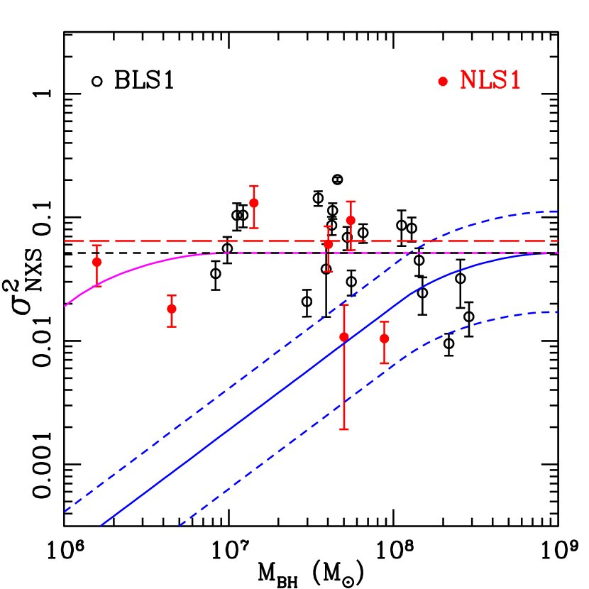
Figure 5: The relationship between the normalized excess variance ($\sigma^{2}_{\rm NXS}$) and black hole mass ($M_{\rm BH}$). It appears that the variance does not depend on the mass. For the PSD predictions shown in this figure, $\nu_{\rm b}$ scales with $M_{\rm BH}$ only, and $C_{\rm b}=43$ Hz $M_{\odot}$ is assumed. The blue solid line is the hard-state PSD prediction with ${\rm{PSD_{amp}}}=0.024$ and $C_{\mathrm{LFB}}=20$. The upper and bottom blue dashed lines correspond to the hard-state PSD predictions by changing the value of ${\rm{PSD_{amp}}}$ to $0.052$ and $0.008$ (keeping $C_{\mathrm{LFB}}=20$), respectively. The magenta solid line shows the hard-state PSD prediction by setting $C_{\mathrm{LFB}}=2000$ (holding ${\rm{PSD_{amp}}}=0.024$). The black dashed line is the soft-state PSD prediction with ${\rm{PSD_{amp}}}=0.024$. The red dashed line shows the averaged value of the observed variances of 27 AGNs, which is the same to the soft-state PSD prediction with ${\rm{PSD_{amp}}}=0.03$ obtained from the average variance with formula [11]. It can be seen that the observed variance-mass relation is much more consistent with the soft-state PSD predictions (independent of mass) than the hard-state PSD predictions. The hard-state PSD prediction also ”fits” the data only by increasing $C_{\mathrm{LFB}}$ by two order of magnitude.

Figure 5 shows the relationship between the estimated $\sigma^{2}_{\rm NXS}$ and $M_{\rm BH}$. BLS1 and NLS1 do not occupy different regions. Although the scatter is large, it appears that the variance does not depend on mass. The Pearson’s correlation coefficient between $\log\sigma^{2}_{\rm NXS}$ and $\log M_{\rm BH}$ is $r=-0.23$, and the null probability is $p=0.25$, suggesting that the variance may not correlate with $M_{\rm BH}$.

The blue solid line in Figure 5 plots the variance-mass relation predicted by the hard-state PSD model, in which we adopt the best fit parameters (${\rm{PSD_{amp}}}=0.024$, $C_{\rm b}=43$ Hz $M_{\odot}$, and $C_{\mathrm{LFB}}=20$) obtained by O’Neill et al. (2005) with the short timescale variance-mass relation. It is clear that the predicted relation is not in agreement with the observed one at all. In fact, the hard-state PSD predicts that the variances linearly increase with mass for $M_{\rm BH}\lesssim 10^{8}M_{\odot}$. The predicted variance-mass relation flattens when $M_{\rm BH}\gtrsim 2\times 10^{8}M_{\odot}$. This means that AGNs of $M_{\rm BH}\lesssim 10^{8}M_{\odot}$ have $\nu_{\rm max}<\nu_{\rm LFB}$, whereas those of $M_{\rm BH}\gtrsim 2\times 10^{8}M_{\odot}$ have $\nu_{\rm min}<\nu_{\rm LFB}<\nu_{\rm max}$.

However, the failure of the hard-state PSD prediction merely shows that a very specific version of the hard-state PSD model does not fit the data. This does not prove that the hard-state PSD model, with another set of parameter values can not fit the data (to some extent). Among the three parameters, $C_{\mathrm{b}}$, the scaling of $\nu_{\rm b}$ with mass, is best determined and mostly impossible to change a lot. As we will discuss in Section 4.3, the value of ${\rm{PSD_{amp}}}$, primarily due to the intrinsic scatter of variance measurements, may range from 0.008 up to 0.052. In Figure 5, we plot again the hard-state PSD predictions by changing the values of ${\rm{PSD_{amp}}}$ to 0.008 and 0.052. The ${\rm{PSD_{amp}}}=0.008$ prediction (the bottom blue dashed line) fails completely. Although the ${\rm{PSD_{amp}}}=0.052$ prediction is on top of the ${\rm{PSD_{amp}}}=0.024$ one, it still can not ”fit” adequately the data. As a result, it is rather unlikely that the hard-state PSD predictions can explain the data by altering the values of ${\rm{PSD_{amp}}}$.

In fact, the hard-state PSD predictions, within the ${\rm{PSD_{amp}}}$ range adopted above, are about $1-2$ order of magnitude smaller than the observed variances for $M_{\rm BH}\lesssim 10^{8}M_{\odot}$. This indicates that, down to frequencies of $\sim 10^{-9}$ Hz, the PSDs of these AGNs should not show the second low-frequency breaks. In order to test this assumption, we show in Figure 5 (the magenta solid line) the hard-state PSD prediction by setting $C_{\mathrm{LFB}}=2000$, which explains the data much better than the case of $C_{\mathrm{LFB}}=20$. Thus, our long timescale variance-mass relation does not favor $C_{\mathrm{LFB}}=20$ assumed by O’Neill et al. (2005) for the short timescale variance-mass relation. However, our data show that the second breaks of AGN PSDs, if exist, should be close to or beyond the frequency of $\nu_{\rm min}\sim 2.27\times 10^{-9}$ Hz. Similarly, the low frequency end reached by the presently known high quality AGN PSDs (e.g., McHardy et al. 2004, 2005) have extended through to $\sim 10^{-8}$ Hz, at which the PSDs do not show the second breaks either. Hence, both the variance and PSD data imply that the ratio of $\nu_{\rm b}$ to $\nu_{\rm LFB}$ should be larger than $\sim 2000$ if the second breaks of AGN PSDs would exist.

The black dashed line in Figure 5 plots the soft-state PSD prediction by using $C_{\rm b}=43$ Hz $M_{\odot}$ and ${\rm{PSD_{amp}}}=0.024$, same as the ones used for the hard-state PSD prediction. The soft-state PSD prediction is independent of mass due to $\nu_{\rm max}<\nu_{\rm b}$ for all of our AGNs, which is roughly in agreement with the data. The mass-independent variance predicted by the soft-state PSD is $5.14\times 10^{-2}$, slightly smaller than the average value ($6.64\times 10^{-2}$, the red dashed line) of the observed variances of 27 AGNs (see Section 4.3). The red dashed line is also identical to the soft-state PSD prediction by using ${\rm{PSD_{amp}}}=0.03$, obtained from the averaged variance with formula [11] (see Section 4.3), and $C_{\rm b}=43$ Hz $M_{\odot}$. Consequently, our long-timescale variance-mass relation seems to favor the soft-state PSD for AGNs.

With the present data, the soft-state PSD prediction is actually identical to the hard-state PSD prediction with $C_{\mathrm{LFB}}\gtrsim 2000$. However, the value of $C_{\mathrm{LFB}}\gtrsim 2000$ is remarkably larger than the currently approved value ($\sim 10-100$) by analogy with the GBH hard-sate PSDs. This suggests that such large value of $C_{\mathrm{LFB}}$ would not be physical for AGNs. As a result, our long timescale variance-mass relation is very likely to agree with the soft-state PSD prediction rather than with the hard-state PSD predictions.

4.2 Relationship between $\sigma^{2}_{\rm NXS}$ and $L_{\rm bol}$

On short timescales, the observed variance anti-correlates with X-ray luminosity of AGNs (e.g., Nandra et al. 1997), whereas it weakly increases with larger bolometric luminosity (Zhou et al. 2010). Figure 6 plots the relationship between our long-timescale $\sigma^{2}_{\rm NXS}$ and $L_{\rm bol}$ for 20 AGNs. It appears that the variance does not depend on $L_{\rm bol}$. The Pearson’s correlation coefficient between $\log\sigma^{2}_{\rm NXS}$ and $\log L_{\rm bol}$ is $r=-0.09$, and the null probability is $p=0.70$, indicating that the variance does not correlate with $L_{\rm bol}$. This independence of variance on bolometric luminosity presents another evidence for the soft-state PSD shape of AGNs. Because all of our AGNs show $\nu_{\rm max}<\nu_{\rm b}$, the soft-state PSD deservedly predicts that the variance is independent of $L_{\rm bol}$, suggesting that formula [8] is consistent with the lack of any correlation between $\sigma^{2}_{\rm NXS}$ and $L_{\rm bol}$. However, the hard-state PSD with $C_{\mathrm{LFB}}=20$ would predict that the variance decreases with increasing bolometric luminosity.

4.3 Scatter of $\sigma^{2}_{\rm NXS}$ and constant ${\rm{PSD_{amp}}}$

For the soft-state PSD model, formula [11] shows that the value of ${\rm{PSD_{amp}}}$ can be directly estimated from the observed variance of an object if its $\nu_{\rm b}$ is larger than $\nu_{\rm max}$. Due to $\nu_{\rm b}>\nu_{\rm max}$ for all objects in our sample, their observed variances, independent of $M_{\rm BH}$ (and $L_{\rm bol}$), are expected to be the same. Therefore, a constant ${\rm{PSD_{amp}}}$ (same for all AGNs) can be obtained with the observed variances of these objects. However, Table 1 (also Figure 5) shows that the observed variances exhibit quite large scatter by about one order of magnitude, indicating that the derived values of ${\rm{PSD_{amp}}}$ have an identical degree of scatter from object to object. This is inconsistent with the assumption that the value of ${\rm{PSD_{amp}}}$ is the same for all AGNs. However, the large scatter of the observed variances is probably due to the intrinsic scatter (probably very large) of the variance measurements (e.g., see Section 5 in Vaughan et al. 2003 and the entries in their Table 1, also see Section 3.2 in O’Neill et al. 2005). Consequently, the scatter of the estimated variances does not imply the intrinsic scatter of ${\rm{PSD_{amp}}}$. The way to reduce the intrinsic scatter of variance measurements is to average a number of estimated variances. As a result, in order to obtain the constant ${\rm{PSD_{amp}}}$ and reduce its uncertainty, we average the observed variances of our 27 AGNs and derive its standard deviation, which is $6.44\pm 4.76\times 10^{-2}$. With formula [11], we obtain ${\rm{PSD_{amp}}}=0.030\pm 0.022$. Based on the short-timescale variance-mass relations, not sensitive to differentiate the soft-state and hard-state PSD predictions, Papadakis (2004) and O’Neill et al. (2005) obtained ${\rm{PSD_{amp}}}\sim 0.02-0.03$, similar to the one we obtained.

The AGN PSDs obtained with high-quality RXTE and XMM-Newton light curves indicate that the values of ${\rm{PSD_{amp}}}$ also show large scatter by up to an order of magnitude for different AGNs (e.g., Markowitz et al. 2003; Done & Gierliński 2005; Uttley & McHardy 2005). Most probably, the uncertainty in the best fit ${\rm{PSD_{amp}}}$ does not indicate a range of intrinsic ${\rm{PSD_{amp}}}$, but rather indicates the true uncertainty with which one can estimate the constant ${\rm{PSD_{amp}}}$ with the present PSDs. Nevertheless, one could average the known values of ${\rm{PSD_{amp}}}$ from the best fits to the high-quality PSDs of a few AGNs as an approximate value of the constant ${\rm{PSD_{amp}}}$. The averaged value of ${\rm{PSD_{amp}}}$ ($\sim 0.02-0.03$) is also similar to the one we obtained from the average of the observed variances of a number of AGNs under the assumption of the soft-state PSD shape.

4.4 The $\sigma^{2}_{\rm NXS}-M_{\rm BH}-L_{\rm bol}$ plane

Formula [8] shows that $\nu_{\rm b}$ depends on both $M_{\rm BH}$ and $L_{\rm bol}$. It is therefore inadequate to study the $\sigma^{2}_{\rm NXS}-M_{\rm BH}$ and $\sigma^{2}_{\rm NXS}-L_{\rm bol}$ relation, respectively. If taking into account the scaling of $\nu_{\rm b}$ with $M_{\rm BH}$ and $L_{\rm bol}$ synchronously, we have to compare the observed variances with the ones predicted by the PSD models, i.e., a projection of the $\sigma^{2}_{\rm NXS}-M_{\rm BH}-L_{\rm bol}$ plane. The predictions are calculated with the soft-state and hard-state PSD, respectively, with the values of $\nu_{\rm b}$ calculated with formula [8] and ${\rm{PSD_{amp}}}=0.03$ estimated in Section 4.3. For the hard-state PSD predictions, $C_{\mathrm{LFB}}$ is still assumed as $20$.

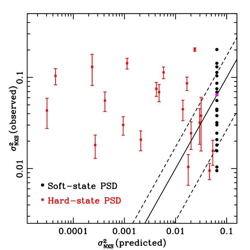
Figure 7: The observed $\sigma^{2}_{\rm NXS}$ is plotted against the predicted $\sigma^{2}_{\rm NXS}$ for the soft-state (black solid circles) and hard-state (red solid squares) PSD models, respectively. For the soft-state and hard-state PSD predictions, we adopt ${\rm{PSD_{amp}}}=0.03$, and the PSD break frequency ($\nu_{\rm b}$) scales with black hole mass and bolometric luminosity via formula [8]. The ratio of $\nu_{\rm b}$ to $\nu_{\rm LFB}$ ($C_{\mathrm{LFB}}$) is assumed to be $20$ for the hard-state PSD model. The black solid line is not a best fit line to the relation between the observed and predicted variances, whereas it is the position on which an object will lie if the predicted variance is equal to the observed one. The two black dashed lines indicate $1\sigma$ deviation from the solid line, representing the positions to which the solid line will shift if the predicted variance is calculated with ${\rm{PSD_{amp}}}=0.052$ (the upper black dashed line) and ${\rm{PSD_{amp}}}=0.008$ (the lower black dashed line), respectively. The predicted variances by the soft-state PSD are the same for all of the objects (the magenta solid circle indicates the averaged value of the observed variances). The error bars on the observed variances are not shown for the soft-state PSD model, but they are identical to the ones for the hard-state PSD model since the observed variances are the same for the two PSD models. Most of AGNs locate far away from the three lines for the hard-state PSD predictions, whereas they lie close to the lines for the soft-state PSD predictions.

Figure 7 plots the observed $\sigma^{2}_{\rm NXS}$ against the predicted $\sigma^{2}_{\rm NXS}$ (the black solid circles for the soft-state PSD predictions and the red solid squares for the hard-state PSD ones) for 20 AGNs. We specially emphasize that the black solid line in Figure 7 is not a best fit line to the relation between the observed and predicted variances (for the two PSD models, respectively). It is the line on which an object will lie exactly if the predicted variance is equal to the observed one. In the same way, the two black dashed lines indicate $1\sigma$ deviations from the black solid line, showing the positions to which the black solid line will shift if the predicted variances are calculated with ${\rm{PSD_{amp}}}=0.052$ (the upper black dashed line) and ${\rm{PSD_{amp}}}=0.008$ (the lower black dashed line), respectively. In other words, the upper and bottom black dashed lines have the exactly same meanings as the black solid line if the (soft-state or hard-state) PSD predictions are calculated with ${\rm{PSD_{amp}}}=0.052$ and ${\rm{PSD_{amp}}}=0.008$, respectively. The two values of ${\rm{PSD_{amp}}}$ are the upper and lower $1\sigma$ deviations from ${\rm{PSD_{amp}}}=0.03$ obtained in Section 4.3.

Due to $\nu_{\rm b}>\nu_{\rm max}$, the predicted variances by the soft-state PSD are the same for all of our AGNs (the magenta solid circle indicates the averaged value of the observed variances). As a result, the relation between the observed and predicted variances is perpendicular to the axis of the predicted variance. Most of the objects lie within the $1\sigma$ range of the black solid line. For the hard-state PSD, however, most of AGNs locate far away from the black solid and dashed lines. Therefore, Figure 7 suggests that the soft-state PSD predictions are much more consistent with the data than the hard-state PSD predictions, but the latter is only for the specific parameters of O’Neill et al. (2005) as already discussed in Section 4.1. Moreover, for the hard-state PSD predictions, the majority of the most massive objects lie close to the black solid line, indicating that their values of $\nu_{\rm min}$ are slightly smaller than the respective values of $\nu_{\rm LFB}$. As a result, these massive AGNs, due to longer timescales, are not good indictors for differentiating the two PSD models.

5 Discussion and conclusions

With the ASM data accumulated over 14 years, we estimate the normalized excess variances of 27 AGNs in the X-ray band on the longest timescale ($\Delta t=300$ days and $T=5100$ days) so far. Although the observed variances show quite large scatter, they appear to not depend on black hole mass and bolometric luminosity of AGNs. This phenomenology has already been noticed by Markowitz & Edelson (2004) with PCA light curves of $\Delta t=34.4$ days and $T=1296$ days. The short-timescale variance-mass relation has been able to constrain the PSD amplitude and the scaling law of the PSD high-break frequency with black hole mass (Papadakis 2004; O’Neill et al. 2005), but it can not be used to effectively distinguish the hard-state and soft-state PSD models hypothesized for AGNs (as they have the same predictions on short timescales) in general. Relatively, the long timescale variance-mass relation is more valid to determine whether the AGN PSDs have the second low-frequency breaks or not.

With the best-fit parameters obtained by O’Neill et al. (2005), the soft-state PSD prediction is much more consistent with our long timescale variance-mass relation than the hard-state PSD prediction. On the longest timescale so far, the hard-state PSD predicts that the variance increases with mass, whereas the soft-state PSD gives the mass-independent variance. In fact, the variances predicted by the hard-state PSD model are remarkably smaller than the observed variances for most of our AGNs. Furthermore, by taking into account the scaling factor of the PSD high-break frequency with black hole mass and bolometric luminosity together, the soft-state PSD predictions are more likely to agree with the observed variances than the hard-state PSD predictions. Therefore, the long timescale variances appear to favor the soft-state rather than the hard-state PSD shape for AGNs. It is reasonable to assume that it is the variances predicted by the best-fit PSD parameters of O’Neill et al. (2005), not by the hard-state PSD in general, that are not consistent with the data. However, we have demonstrated that changes of PSD amplitude within the most possible range do not improve the ”fit” to the data. Rather, the hard-state PSD model could probably agree with the data, but it would require a range of PSD amplitude values that have not been observed so far in the cases when a proper fitting has been done to the PSDs of a few sources. Despite the hard-state PSD predictions with $\nu_{\rm b}/\nu_{\rm LFB}\gtrsim 2000$ can explain the data as good as the soft-state PSD predictions, such large value of $\nu_{\rm b}/\nu_{\rm LFB}$ is very probably nonexistent by scaling from GBHs to AGNs. Moreover, the hard-state PSD with $\nu_{\rm b}/\nu_{\rm LFB}\gtrsim 2000$ is actually identical to the soft-state PSD for the present data.

Up to now, the best fits show that the high-quality PSDs of a few AGNs have one high-frequency break only except for Ark 564 who exhibits the second low-frequency break. Thereby, our variance analysis of a larger sample of AGNs agrees with the direct PSD analysis of a smaller sample of AGNs, both implying the soft-state PSD shape for AGNs. For example, the PSDs of NGC 4051 and MCG-6-30-15, having the smallest mass among our sample, show one break only down to frequency of $\sim 10^{-8}$ Hz at quite high confidence level (McHardy et al. 2004; 2005). At the same time, Figure 5 shows that the estimated variances of the two objects, roughly consistent with the soft-state PSD predictions, are remarkably larger than the variances predicted by the hard-state PSD model. Compared to the PSD analysis, however, our variance analysis lowers the frequencies by more than one order of magnitude. Therefore, our results further strengthen the standpoint, first suggested by the PSD analysis, that AGN PSDs might have one break only.

By analogy with the PSDs of GBHs in the high/soft state, both the variance and PSD analyzes suggest that Seyfert-type AGNs are in the high accretion state. Therefore, AGNs are thought to be scaled-up GBHs in the high/soft state, characterized by the PSD break frequency scaling with black hole mass and bolometric luminosity (or Eddington accretion rate) from GBHs to AGNs (McHardy et al. 2006). Under these assumptions, the break frequencies of all AGNs in our sample are substantially smaller than the maximum frequency to which the 300-day binned light curves correspond, indicating that the estimated variances are the same for our AGNs. This motivate us to average the observed variances, from which we obtain a constant PSD amplitude of $\sim 0.030\pm 0.022$ for AGNs, roughly consistent with those obtained from the direct PSD analysis and the short-timescale variance analysis.

There are a number of factors which may cause the large scatter of the observed variances. One main effect may come from the low quality ASM light curves for AGNs (see Section 2). From the point view of PSD itself, the slope above and below the break frequency are not exactly equal to $-2$ and $-1$ for most of AGNs, as already seen from the known AGN PSDs (e.g., Uttley, McHardy & Papadakis 2002). At the same time, the AGN PSDs are better described by a bending power law (e.g., Uttley & McHardy 2005) rather than by an abruptly broken power law assumed here for simplicity. It is worth noting that, if the soft-state PSD model is applicable to AGNs, the observed variances should be the same. However, because the variance measurements have the known intrinsic scatter (Vaughan et al. 2003; O’Neill et al. 2005), which could be very large, the large scatter of the estimated excess variances is almost certainly due to the intrinsic scatter of the $\sigma^{2}_{\rm NXS}$ values themselves. In order to decrease the intrinsic scatter of variance measurements, it is necessary to perform high quality observations on longer timescale (and/or multiple observations) for AGNs. Averaging the multiple variances of an object (from segments of long-timescale or multiple observations) can reduce the intrinsic uncertainty of variance measurements. Due to shorter timescales, the AGNs with smaller or intermediate black hole mass are more effective to differentiate the two PSD models.

In conclusion, the longest timescale X-ray variability suggests that AGN PSDs have one break only, and further indicates that AGNs are in the high accretion state.

Table 1: The AGN sample and relevant parameters

Source	ASM	$\sigma^{2}_{\rm NXS}$	$M_{\rm BH}$	ref.,	$T_{\rm b}$	ref.	$L_{\rm bol}$	ref.
Name	rate	($\times 10^{-2}$)	($10^{7}M_{\odot}$)	meth.	(day)		(${\rm ergs~{}s^{-1}}$)
Broad line objects
3C 120	0.22	3.01$\pm$0.69	5.55	1,r	…	…	45.34	9
3C 390.3	0.16	1.57$\pm$0.48	28.7	1,r	…	…	44.88	9
Ark 120	0.17	2.44$\pm$0.82	15.0	1,r	…	…	44.91	9
Fairall 9	0.13	3.20$\pm$1.35	25.5	1,r	28.9	14	45.23	9
IC 4329a	0.51	0.95$\pm$0.19	21.7	2,d	4.6	2	44.78	9
MR 2251-178	0.19	3.51$\pm$0.92	0.83	3,o	…	…	…	…
Mrk 79	0.14	6.89$\pm$1.47	5.24	1,r	…	…	44.57	9
Mrk 279	0.12	14.3$\pm$1.95	3.49	1,r	…	…	…	…
Mrk 290	0.09	10.4$\pm$2.59	1.12	4,o	…	…	…	…
Mrk 509	0.19	4.49$\pm$1.13	14.3	1,r	…	…	45.03	9
NGC 526a	0.13	8.16$\pm$1.81	12.9	3,o	…	…	…	…
NGC 985	0.10	8.62$\pm$2.78	11.2	4,o	…	…	…	…
NGC 3227	0.18	8.63$\pm$1.45	4.22	1,r	0.59	14	43.86	9
NGC 3516	0.13	11.3$\pm$1.65	4.27	1,r	5.8	14	44.29	9
NGC 3783	0.27	2.08$\pm$0.51	2.98	1,r	2.9	14	44.41	9
NGC 4151	0.42	20.2$\pm$0.86	4.57	5,r	9.2	14	43.73	9
NGC 4258	0.09	3.81$\pm$2.25	3.90	6,m	513	14	43.45	9
NGC 4593	0.16	5.58$\pm$1.35	0.98	7,r	…	…	44.09	9
NGC 5548	0.19	7.51$\pm$1.31	6.54	8,r	18.3	14	44.83	9
NGC 7469	0.14	10.4$\pm$2.11	1.22	1,r	…	…	45.28	9
Narrow line objects
IC 5063	0.08	9.44$\pm$4.02	5.50	9,d	…	…	44.53	9
MCG-6-30-15	0.27	1.81$\pm$0.52	0.45	10,o	0.15	14	43.56	14
Mrk 335	0.07	13.1$\pm$4.88	1.42	1,r	0.068	15	44.69	9
Mrk 478	0.09	6.05$\pm$2.41	4.02	11,o	…	…	…	…
NGC 4051	0.12	4.34$\pm$1.58	0.16	12,r	0.019	14	43.56	9
NGC 5506	0.29	1.04$\pm$0.39	8.80	11,d	0.89	14	44.47	14
PKS 0558-504	0.11	1.07$\pm$0.88	4.50	13,o	…	…	…	…

Figure 1: The ASM light curve for the lowest count rate object Mrk 335. The left plot shows the one-day averaged light curve (black solid circles whose errors are not shown for clarity) with the 300-day averaged light curve (red solid squares whose errors are smaller than the symbol size) plotted on top. The right plot presents again the 300-day averaged light curve for clearly showing the source’s variations on timescale of 300 days.

Figure 2: Same to Figure 1 but for the highest count rate object IC 4329a.

Figure 3: The PCA (red solid squares whose errors are smaller than the symbol size) and ASM (black solid circles) 300-day averaged light curves in the time interval over which the long-term PCA observations were performed. For direct comparisons, both light curves are normalized to their respective mean count rates. Left plot is for IC 4329a, and right plot for NGC 3227. Although the differences are present for some time points, the ASM light curves could be considered to roughly follow the PCA ones.

Figure 4: The probability distribution (the black solid line) of $\sigma^{2}_{\rm NXS,b}$ estimated from the simulated light curves of 5100-day long and 300-day binsize. The blue long-dashed line indicates the median of the distribution. The red short-dashed line presents the value of the integral of the intrinsic PSD from $\nu_{\rm min}=1/T$ to $\nu_{\rm max}=1/(2\Delta t)$, where $T=5100$ days and $\Delta t=300$ days.

Figure 6: The relationship between the normalized excess variance ($\sigma^{2}_{\rm NXS}$) and bolometric luminosity ($L_{\rm bol}$). The variance appears to be independent of luminosity.

References

- (1) Arévalo, P., McHardy, I.M., & Summons, D.P. 2008, MNRAS, 388, 211
- (2) Axelsson, M., Borgonovo, L., & Larsson, S. 2006, A&A, 452, 975
- (3) Bentz, M.C., et al. 2006, ApJ, 651, 775
- (4) Bentz, M.C., et al. 2007, ApJ, 662, 205
- (5) Bian, W., & Zhao, Y. 2003, MNRAS, 343, 164
- (6) Done, C., & Gierliński, M. 2005, MNRAS, 364, 208
- (7) Gierliński, M., Nikolajuk, M., & Czerny, B. 2008, MNRAS, 383, 741
- (8) Herrnstein, J.R., Greenhill, L.J., Moran, J.M., Diamond, P.J., Inoue, M., Nakai, N., & Miyoshi, M. 1998, ApJ, 497, 69
- (9) Denney, K.D., et al. 2006, ApJ, 653, 152
- (10) Denney, K.D., et al. 2009, ApJ, 702, 1353
- (11) Klein-Wolt, M., & van der Klis, M. 2008, ApJ, 675, 1407
- (12) Liu, Y., & Zhang, S.N. 2008, A&A, 480, 699
- (13) Lu, Y., & Yu, Q. 2001, MNRAS, 324, 653
- (14) Maccarone, T.J., Gallo, E., & Fender, R. 2003, MNRAS, 345, L19
- (15) Markowitz, A. 2009, ApJ, 698, 1740
- (16) Markowitz, A., & Edelson, R. 2004, ApJ, 617, 939
- (17) Markowitz, A., et al. 2003, ApJ, 593, 96
- (18) McHardy, I.M., Papadakis, I.E., Uttley, P., Page, M.J., & Mason, K.O. 2004, MNRAS, 348, 783
- (19) McHardy, I.M., Gunn, K.F., Uttley, P., & Goad, M.R. 2005, MNRAS, 359, 1469
- (20) McHardy, I.M., Koerding, E., Knigge, C., Uttley, P., & Fender, R.P. 2006, Nature, 444, 730
- (21) McHardy, I.M., et al. 2007, MNRAS, 2007, 382, 985
- (22) Morales, R., & Fabian, A.C. 2002, MNRAS, 329, 209
- (23) Miniutti, G., Ponti, G., Greene, J. E., Ho, L. C., Fabian, A.C., & Iwasawa, K. 2009, MNRAS, 394, 443
- (24) Nandra, K., George, I.M., Mushotzky, R.F., Turner, T.J., & Yaqoob, T. 1997, ApJ, 476, 70
- (25) Nikolajuk, M., Papadakis, I.E., & Czerny, B. 2004, MNRAS, 350, L26
- (26) Nikolajuk, M., Czerny, B., Ziólkowski, J., & Gierliński, M. 2006, MNRAS, 370, 1534
- (27) Nikolajuk, M., Czerny, B., & Gurynowicz, P. 2009, MNRAS, 394, 2141
- (28) O’Neill, P.M., Nandra, K., Papadakis, I.E., & Turner, T.J. 2005, MNRAS, 358, 1405
- (29) Peterson, B.M., et al. 2004, ApJ, 613, 682
- (30) Papadakis, I.E., Brinkmann, W., Negoro, H., & Gliozii, M. 2002, A&A, 382, L1
- (31) Papadakis, I.E. 2004, MNRAS, 348, 207
- (32) Papadakis, I.E., Chatzopoulos, E., Athanasiadis, D., Markowitz, A., & Georgantopoulos, I. 2008a, A&A, 487, 475
- (33) Papadakis, I.E., Ioannou, Z., Brinkmann, W., & Xilouris, E.M. 2008b, A&A, 490, 995
- (34) Pottschmidt, K., Wilms, J., Nowak, M.A., Pooley, G.G., Gleissner, T., Heindl, W.A., Smith, D.M., Remillard, R., Staubert, R. 2003, A&A, 407, 1039
- (35) Pounds, K., Edelson, R., Markowitz, A., & Vaughan, S. 2001, ApJ, 550, L15
- (36) Reynolds, C.S. 1997, MNRAS, 286, 513
- (37) Romano, P., et al. 2004, ApJ, 602, 635
- (38) Summons, D.P., Arévalo, P., McHardy, I.M., Uttley, P., & Bhaskar, A. 2007, MNRAS, 378, 649
- (39) Timmer, J., & Knig, M. 1995, A&A, 300, 707
- (40) Uttley, P., McHardy, I.M., & Papadakis, I.E. 2002, MNRAS, 332, 231
- (41) Uttley, P., & McHardy, I.M. 2005, MNRAS, 363, 586
- (42) Vaughan, S., Edelson, R., Warwick, R.S., & Uttley, P. 2003, MNRAS, 345, 1271
- (43) Wang, T.G., Matsuoka, M., Kubo, H., Mihara, T., & Negoro, H. 2001, ApJ, 554, 233
- (44) Woo, J.H., & Urry, C.M. 2002, ApJ, 579, 530
- (45) Zhang, Y.H. 2002, MNRAS, 337, 609
- (46) Zhang, Y.H., Treves, A., Celotti, A., Qin, Y.P., & Bai, J.M. 2005, ApJ, 629, 686
- (47) Zhang, Y.H., et al. 2002, ApJ, 572, 762
- (48) Zhang, Y.H., Cagnoni, I., Treves, A., Celotti, A., & Maraschi, L. 2004, ApJ, 605, 98
- (49) Zhou, X.L., Zhang, S.N., Wang, D.X., & Zhu, L. 2010, ApJ, 710, 16