Chameleon dark energy models with characteristic signatures

Abstract

In chameleon dark energy models, local gravity constraints tend to rule out parameters in which observable cosmological signatures can be found. We study viable chameleon potentials consistent with a number of recent observational and experimental bounds. A novel chameleon field potential, motivated by $f(R)$ gravity, is constructed where observable cosmological signatures are present both at the background evolution and in the growth-rate of the perturbations. We study the evolution of matter density perturbations on low redshifts for this potential and show that the growth index today $\gamma_{0}$ can have significant dispersion on scales relevant for large scale structures. The values of $\gamma_{0}$ can be even smaller than $0.2$ with large variations of $\gamma$ on very low redshifts for the model parameters constrained by local gravity tests. This gives a possibility to clearly distinguish these chameleon models from the $\Lambda$-Cold-Dark-Matter ($\Lambda$CDM) model in future high-precision observations.

I Introduction

The accelerated expansion of the Universe today is a very important challenge faced by cosmologists review . For an isotropic comoving perfect fluid, a substantially negative pressure is required to give rise to the cosmic acceleration. One of the simplest candidates for dark energy is the cosmological constant with an equation of state $w_{\rm DE}=-1$, but we generally encounter a problem to explain its tiny energy density consistent with observations Weinberg .

There are alternative models of dark energy to the cosmological constant scenario. One of such models is quintessence based on a minimally coupled scalar field with a self-interacting potential quin . In order to realize the cosmic acceleration today, the mass of quintessence is required to be very small ($m_{\phi}\approx 10^{-33}$ GeV). From a viewpoint of particle physics, such a light scalar field may mediate a long range force with standard model particles Carroll . For example, the string dilaton can lead to the violation of equivalence principle through the coupling with baryons Gas . In such cases we need to find some mechanism to suppress the fifth force for the consistency with local gravity experiments.

There are several different ways to screen the field interaction with baryons. One is the so-called run away dilaton scenario Piazza in which the field coupling $F(\phi)$ with the Ricci scalar $R$ is assumed to approach a constant value as the dilaton $\phi$ grows in time (e.g., $F(\phi)=C_{1}+C_{2}e^{-\phi}$ as $\phi\to\infty$). Another way is to consider a field potential having a large mass in the region of high density where local gravity experiments are carried out. In this case the field does not propagate freely in the local region, while on cosmological scales the field mass can be light enough to be responsible for dark energy.

The latter scenario is called the chameleon mechanism in which a density-dependent matter coupling with the field can allow the possibility to suppress an effective coupling between matter and the field outside a spherically symmetric body Khoury1 ; Khoury2 . The chameleon mechanism can be applied to some scalar-tensor theories such as $f(R)$ gravity fRlgc1 ; fRlgc2 and Brans-Dicke theory TUMTY . In $f(R)$ gravity, for example, there have been a number of viable dark energy models fRviable that can satisfy both cosmological and local gravity constraints. For such models the potential of an effective scalar degree of freedom (called “scalaron” star80 ) in the Einstein frame is designed to have a large mass in the region of high density. Even with a strong coupling between the scalaron and the baryons ($Q=-1/\sqrt{6}$), the chameleon mechanism allows the $f(R)$ models to be consistent with local gravity constraints.

The chameleon models are a kind of coupled quintessence models Amendola99 defined in the Einstein frame Khoury1 ; Khoury2 . While the gravitational action is described by the usual Einstein-Hilbert action, non-relativistic matter components are coupled to the Einstein frame metric multiplied by some conformal factor which depends on a scalar (chameleon) field. This is how the gravitational force felt by matter is modified. While there have been many studies for experimental and observational aspects of the chameleon models Brax:2004qh -Brax:2010kv , it is not clear which chameleon potentials are viable if the same field is to be responsible for dark energy.

In this paper we identify a number of chameleon potentials that can be consistent with dark energy as well as local gravity experiments. We then constrain the viable model parameter space by using the recent experimental and observational bounds– such as the 2006 Eöt-Wash experiment Kapner:2006si , the Lunar Laser Ranging experiment Will and the WMAP constraint on the time-variation of particle masses wmap_constraints . This can actually rule out some of the chameleon potentials with natural model parameters for the matter coupling $Q$ of the order of unity.

In order to distinguish the viable chameleon dark energy models from the $\Lambda$CDM model, it is crucial to study both the modifications in the evolution of the background cosmology and the modified evolution of the cosmological density perturbations. For the former, we shall consider the evolution of the so-called statefinders introduced in Refs. Sahni1 ; Sahni2 and show that these parameters can exhibit a peculiar behavior different from those in the $\Lambda$CDM model.

On the other hand, the growth “index” $\gamma$ of matter perturbations $\delta_{m}$ defined through ${\rm d}\ln\delta_{m}/{\rm d}\ln a=(\Omega_{m}^{*})^{\gamma}$, where $a$ is a scale factor and $\Omega_{m}^{*}$ is the density parameter of non-relativistic matter, is an important quantity that allows to discriminate between different dark energy models and interest in this quantity was revived in the context of dark energy models Stein ; Linder .

Its main importance for the study of dark energy models stems from the fact that for $\Lambda$CDM the quantity $\gamma$ is known to be nearly constant with respect to the redshift $z$, i.e. $\gamma_{\Lambda{\rm CDM}}=\gamma_{0}-0.02z$ to exquisite accuracy PG07 , with $\gamma_{0}\equiv\gamma(z=0)\approx 0.555$ Stein . As emphasized in Ref. PG07 , large variations of $\gamma$ on low redshifts could signal that we are dealing with a dark energy model outside General Relativity. This was indeed found for some scalar-tensor dark energy models GP08 and $f(R)$ models GMP08 ; MSY10 ; Narikawa . Such large variations can also occur in models where dark energy interacts with matter ASS09 ; HWJ09 . This is exactly the case in chameleon models, which we investigate in this paper, because of the direct coupling between the chameleon field $\phi$ and all dust-like matter. This direct coupling is however not confined to the dark sector as in standard coupled quintessence.

An additional important point is the possible appearance of a scale-dependence or dispersion in $\gamma$. Hence the behavior of $\gamma$ on low redshifts can be both time-dependent and scale-dependent GMP09 ; Tsujikawa:2009ku ; BT10 . This dispersion can also be present in the models investigated here. Using the observations of large scale structure and weak lensing surveys, one can hope to detect such peculiar behaviors of $\gamma$ (see e.g., Ref. Euclid ). If this is the case this would signal that the gravitational law may be modified on scales relevant to large scale structures Linder ; Gannouji ; Luca ; Tsujikawa:2009ku ; Koivisto ; Nesseris ; BT10 ; SD09 ; Mota:2007zn .

In this paper we study the evolution of $\gamma$ as well as its dispersion, its dependence on the wavenumbers of perturbations. We shall show that some of the chameleon models investigated here can be clearly distinguished from $\Lambda$CDM through the behavior of $\gamma$ exhibiting both large variations and significant dispersion, with the possibility to obtain small values of $\gamma$ today as low as $\gamma_{0}\lesssim 0.2$.

II Chameleon cosmology

II.1 Background equations

In this section we review the basic background evolution of chameleon cosmology. We consider the chameleon theory described by the following action Khoury1 ; Khoury2 ; EP00

$$\mathcal{S}\, = \,\int{{\rm d}^{4}x}\sqrt{-g}\left[\frac{R}{16\pi G}-\frac{1}{2}g^{\mu\nu}\partial_{\mu}\phi\ \partial_{\nu}\phi-V(\phi)\right]$$ (1)

$$+\mathcal{S}_{m}\left[\Psi_{m};A^{2}(\phi)\,g_{\mu\nu}\right]\,,$$

where $g$ is the determinant of the (Einstein frame) metric $g_{\mu\nu}$, $R$ is the Ricci scalar, $G$ is the bare gravitational constant, $\phi$ is a scalar field with a potential $V(\phi)$, and $\mathcal{S}_{m}$ is the matter action with matter fields $\Psi_{m}$. At low redshifts it is sufficient to consider only non-relativistic matter (cold dark matter and baryons), but for a general dynamical analysis including high redshifts radiation must be included.

We assume that non-relativistic matter is universally coupled to the (Jordan frame) metric $A^{2}(\phi)~{}g_{\mu\nu}$, the Einstein frame metric $g_{\mu\nu}$ multiplied by a field-dependent (conformal) factor $A^{2}(\phi)$. This direct coupling to the field $\phi$ is how the gravitational interaction is modified. We can generalize this to arbitrary functions $A^{(i)}(\phi)$ for each matter component $\rho_{i}$, but in this work we will take the same function $A(\phi)$ for all components. We write the function $A(\phi)$ in the form

$$A(\phi)=e^{Q\phi/M_{\rm pl}}\,,$$ (2)

where $M_{\rm pl}=1/\sqrt{8\pi G}$ is the reduced Planck mass and $Q$ describes the strength of the coupling between the field $\phi$ and non-relativistic matter. In the following we shall consider the case in which $Q$ is constant. In fact, the constant coupling arises for Brans-Dicke theory by a conformal transformation to the Einstein frame Khoury2 ; TUMTY . Even when $|Q|$ is of the order of unity, it is possible to make the effective coupling between the field and matter small through the chameleon mechanism.

Let us consider the scalar field $\phi$ together with non-relativistic matter (density $\rho^{*}_{m}$) and radiation (density $\rho_{r}$) in a spatially flat Friedmann-Lemaître-Robertson-Walker (FLRW) space-time with a time-dependent scale factor $a(t)$ and a metric

$${\rm d}s^{2}=g_{\mu\nu}\,{\rm d}x^{\mu}\,{\rm d}x^{\nu}=-{\rm d}t^{2}+a^{2}(t)\,{\rm d}{\bm{x}}^{2}\,.$$ (3)

The corresponding background equations are given by

$$3H^{2}=\left(\rho_{\phi}+\rho_{m}^{*}+\rho_{r}\right)/M_{\rm pl}^{2}\,,$$ (4)

$$\ddot{\phi}+3H\dot{\phi}+V_{,\phi}=-Q\rho_{m}^{*}/M_{\rm pl}\,,$$ (5)

$$\dot{\rho}_{m}^{*}+3H\rho_{m}^{*}=Q\rho_{m}^{*}\dot{\phi}/M_{\rm pl}\,,$$ (6)

$$\dot{\rho}_{r}+4H\rho_{r}=0\,,$$ (7)

where $\rho_{\phi}\equiv\dot{\phi}^{2}/2+V(\phi)$, $V_{,\phi}\equiv{\rm d}V/{\rm d}\phi$, and a dot represents a derivative with respect to cosmic time $t$. The quantity $\rho^{*}_{m}$ is the energy density of non-relativistic matter in the Einstein frame and we have kept the star to avoid any confusion. Integration of Eq. (6) gives the solution $\rho_{m}^{*}\propto a^{-3}e^{Q\phi/M_{\rm pl}}$. We define the conserved matter density:

$$\rho_{m}\equiv e^{-Q\phi/M_{\rm pl}}\rho_{m}^{*}\,,$$ (8)

which satisfies the standard continuity equation, $\dot{\rho}_{m}+3H\rho_{m}=0$. Then the field equation (5) can be written in the form

$$\ddot{\phi}+3H\dot{\phi}+V_{{\rm eff},\phi}=0\,,$$ (9)

where $V_{\rm eff}$ is the effective potential defined by

$$V_{\rm eff}\equiv V(\phi)+e^{Q\phi/M_{\rm pl}}\rho_{m}\,.$$ (10)

We emphasize that it is the Einstein frame which is the physical frame. Due to the coupling between the field and matter, particle masses do evolve with time in our model.

We consider runaway positive potentials $V(\phi)$ in the region $\phi>0$, which monotonically decrease and have a positive mass squared, i.e. $V_{,\phi}<0$ and $V_{,\phi\phi}>0$. We also demand the following conditions

$$\lim_{\phi\to 0}\left|\frac{V_{,\phi}}{V}\right|=\infty\,,\qquad\lim_{\phi\to\infty}\frac{V_{,\phi}}{V}=0\,.$$ (11)

The former is required to have a large mass in the region of high density, whereas we need the latter condition to realize the late-time cosmic acceleration in the region of low density. At $\phi=0$ the potential approaches either $\infty$ or a finite positive value $V_{0}$. In the limit $\phi\to\infty$ we have either $V\to 0$ or $V\to V_{\infty}$, where $V_{\infty}$ is a nonzero positive constant. If $Q>0$ the effective potential $V_{\rm eff}(\phi)$ has a minimum at the field value $\phi_{m}~{}(>0)$ satisfying the condition $V_{{\rm eff},\phi}(\phi_{m})=0$, i.e.

$$V_{,\phi}(\phi_{m})+Q(\rho_{m}/M_{\rm pl})e^{Q\phi_{m}/M_{\rm pl}}=0\,.$$ (12)

If the potential satisfies the conditions $V_{,\phi}>0$ and $V_{,\phi\phi}>0$ in the region $\phi<0$, there exists a minimum at $\phi=\phi_{m}~{}(<0)$ provided that $Q<0$. In fact this situation arises in the context of $f(R)$ dark energy models fRlgc1 ; fRlgc2 . Since the analysis in the latter is equivalent to that in the former, we shall focus on the case $Q>0$ and $V_{,\phi}<0$ in the following discussion.

II.2 Dynamical system

In order to discuss cosmological dynamics, it is convenient to introduce the following dimensionless variables

$$x_{1}\equiv\frac{\dot{\phi}}{\sqrt{6}HM_{\rm pl}}\,,\quad x_{2}\equiv\frac{\sqrt{V}}{\sqrt{3}HM_{\rm pl}}\,,\quad x_{3}\equiv\frac{\sqrt{\rho_{r}}}{\sqrt{3}HM_{\rm pl}}\,.$$ (13)

Equation (4) expresses the constraint existing between these variables, i.e.

$$\Omega_{m}^{*}\equiv\frac{\rho_{m}^{*}}{3H^{2}M_{\rm pl}^{2}}=1-\Omega_{\phi}-\Omega_{r}\,,$$ (14)

where

$$\Omega_{\phi}\equiv x_{1}^{2}+x_{2}^{2}\,,\qquad\Omega_{r}\equiv x_{3}^{2}\,.$$ (15)

Taking the time-derivative of Eq. (4) and making use of Eqs. (5)-(7), it is straightforward to derive the following equation

$$\frac{H^{\prime}}{H}=-\frac{1}{2}\left(3+3x_{1}^{2}-3x_{2}^{2}+x_{3}^{2}\right)\,,$$ (16)

where a prime represents a derivative with respect to $N\equiv\ln a$. A useful quantity is the effective equation of state

$$w_{{\rm eff}}=-1-\frac{2}{3}\frac{H^{\prime}}{H}=x_{1}^{2}-x_{2}^{2}+\frac{x_{3}^{2}}{3}\,.$$ (17)

We also introduce the field equation of state $w_{\phi}$, as

$$w_{\phi}\equiv\frac{\dot{\phi}^{2}/2-V(\phi)}{\dot{\phi}^{2}/2+V(\phi)}=\frac{x_{1}^{2}-x_{2}^{2}}{x_{1}^{2}+x_{2}^{2}}\,.$$ (18)

Using Eqs. (4)-(7), we obtain the following equations

$$x_{1}^{\prime}=-3x_{1}+\frac{\sqrt{6}}{2}\lambda x_{2}^{2}-x_{1}\frac{H^{\prime}}{H}$$

$$~{}~{}~{}~{}~{}~{}-\frac{\sqrt{6}}{2}Q\left(1-x_{1}^{2}-x_{2}^{2}-x_{3}^{2}\right)\,,$$ (19)

$$x_{2}^{\prime}=-\frac{\sqrt{6}}{2}\lambda x_{1}x_{2}-x_{2}\frac{H^{\prime}}{H}\,,$$ (20)

$$x_{3}^{\prime}=-2x_{3}-x_{3}\frac{H^{\prime}}{H}\,,$$ (21)

$$\lambda^{\prime}=-\sqrt{6}\lambda^{2}(\Gamma-1)x_{1}\,,$$ (22)

where

$$\lambda\equiv-\frac{M_{\rm pl}V_{,\phi}}{V}\,,\qquad\Gamma\equiv\frac{VV_{,\phi\phi}}{V_{,\phi}^{2}}\,.$$ (23)

From the conditions (11) it follows that the quantity $\lambda$ decreases from $\infty$ to 0 as $\phi$ grows from 0 to $\infty$. Since $x_{1}>0$ in Eq. (22), the condition $\lambda^{\prime}<0$ translates into

$$\Gamma=\frac{VV_{,\phi\phi}}{V_{,\phi}^{2}}>1\,.$$ (24)

Chameleon potentials shallower than the exponential potential ($\Gamma=1$) can satisfy this condition.

Once the field settles down at the minimum of the effective potential (10), we have

$$x_{1}\simeq 0\,,\qquad x_{2}\simeq\sqrt{\frac{Q}{\lambda}\Omega_{m}^{*}}\,,$$ (25)

which gives $w_{\phi}\simeq-1$ from Eq. (18). As the matter density $\rho^{*}_{m}$ decreases, the field evolves slowly along the instantaneous minima characterized by (25). We require that $\lambda\gg Q={\cal O}(1)$ during radiation and deep matter eras for consistency with local gravity constraints in the region of high density. For the dynamical system (19)-(22) there is another fixed point called the “$\phi$-matter-dominated era ($\phi$MDE)” Amendola99 where $\Omega_{\phi}=w_{\rm eff}=2Q^{2}/3$. However, since we are considering the case in which $Q$ is of the order of unity, the effective equation of state $w_{\rm eff}$ is too large to be compatible with observations. Only when $Q<{\cal O}(0.1)$ the $\phi$MDE can be responsible for the matter era Amendola99 .

When the chameleon is slow-rolling along the minimum, we obtain the following relation from Eqs. (15) and (25):

$$\frac{\lambda}{Q}\simeq\frac{\Omega_{m}^{*}}{\Omega_{\phi}}\,.$$ (26)

While $\lambda\gg Q$ during the radiation and matter eras, $\lambda$ becomes the same order as $Q$ around the present epoch. The field potential is the dominant contribution on the r.h.s. of Eq. (4) today, so that

$$V(\phi_{0})\simeq 3H_{0}^{2}M_{\rm pl}^{2}\simeq\rho_{c}\,,$$ (27)

where the subscript “0” represents present values and $\rho_{c}\simeq 10^{-29}$ g/cm³ is the critical density today.

III Chameleon mechanism

In this section we review the chameleon mechanism as a way to escape local gravity constraints. In addition to the cosmological constraints discussed in the previous section, this will enable us to restrict the forms of chameleon potentials.

Let us consider a spherically symmetric space-time in the weak gravitational background with the neglect of the backreaction of metric perturbations. As in the previous section we consider the case in which couplings $Q_{i}$ are the same for each matter component ($Q_{i}=Q$), i.e., in which the function $A(\phi)$ is given by Eq. (2). Varying the action (1) with respect to $\phi$ in the Minkowski background, we obtain the field equation

$$\frac{{\rm d}^{2}\phi}{{\rm d}r^{2}}+\frac{2}{r}\frac{{\rm d}\phi}{{\rm d}r}=\frac{{\rm d}V_{{\rm eff}}}{{\rm d}\phi}\,,$$ (28)

where $r$ is the distance from the center of symmetry and $V_{\rm eff}$ is defined in Eq. (10).

Assuming that a spherically symmetric object (radius $r_{c}$ and mass $M_{c}$) has a constant density $\rho_{m}=\rho_{A}$ with a homogeneous density $\rho_{m}=\rho_{B}$ outside the body, the effective potential has two minima at $\phi=\phi_{A}$ and $\phi=\phi_{B}$ satisfying the conditions

$$V_{,\phi}(\phi_{A}) + Q(\rho_{A}/M_{\rm pl})e^{Q\phi_{A}/M_{\rm pl}}=0\,,$$ (29)

$$V_{,\phi}(\phi_{B}) + Q(\rho_{B}/M_{\rm pl})e^{Q\phi_{B}/M_{\rm pl}}=0\,.$$ (30)

Since $Q\phi_{A}/M_{\rm pl}\ll 1$ and $Q\phi_{B}/M_{\rm pl}\ll 1$ for viable field potentials in the regions of high density, the conserved matter density $\rho_{m}$ is practically indistinguishable from the matter density $\rho_{m}^{*}$ in the Einstein frame.

The field profile inside and outside the body can be found analytically. Originally this was derived in Refs. Khoury1 ; Khoury2 under the assumption that the field is frozen around $\phi=\phi_{A}$ in the region $0<r<r_{1}$, where $r_{1}~{}(<r_{c})$ is the distance at which the field begins to evolve. It is possible, even without this assumption, to derive analytic solutions by considering boundary conditions at the center of the body Tamaki:2008mf .

We consider the case in which the mass squared $m_{B}^{2}\equiv\frac{{\rm d}^{2}V_{\rm eff}}{{\rm d}\phi^{2}}(\phi_{B})$ outside the body satisfies the condition $m_{B}r_{c}\ll 1$, so that the $m_{B}$-dependent terms can be negligible when we match solutions at $r=r_{c}$. The resulting field profile outside the body ($r>r_{c}$) is given by Tamaki:2008mf

$$\phi(r)=\phi_{B}-\frac{Q_{{\rm eff}}}{4\pi M_{\rm pl}}\frac{M_{c}}{r}\,,$$ (31)

where the effective coupling $Q_{\rm eff}$ between the field and matter is

$$Q_{{\rm eff}} = Q\biggl{[}1-\frac{r_{1}^{3}}{r_{c}^{3}}+3\frac{r_{1}}{r_{c}}\frac{1}{(m_{A}r_{c})^{2}}$$ (32)

$$~{}~{}~{}\times\left\{\frac{m_{A}r_{1}(e^{m_{A}r_{1}}+e^{-m_{A}r_{1}})}{e^{m_{A}r_{1}}-e^{-m_{A}r_{1}}}-1\right\}\biggr{]}\,.$$

The mass $m_{A}$ is defined by $m_{A}^{2}\equiv\frac{{\rm d}^{2}V_{\rm eff}}{{\rm d}\phi^{2}}(\phi_{A})$. The distance $r_{1}$ is determined by the condition $m_{A}^{2}\left[\phi(r_{1})-\phi_{A}\right]=Q\rho_{A}$, which translates into

$$\phi_{B}-\phi_{A}+Q\rho_{A}(r_{1}^{2}-r_{c}^{2})/(2M_{\rm pl})$$

$$=\frac{6QM_{\rm pl}\Phi_{c}}{(m_{A}r_{c})^{2}}\frac{m_{A}r_{1}(e^{m_{A}r_{1}}+e^{-m_{A}r_{1}})}{e^{m_{A}r_{1}}-e^{-m_{A}r_{1}}}\,,$$ (33)

where $\Phi_{c}=M_{c}/(8\pi r_{c})=\rho_{A}r_{c}^{2}/(6M_{\rm pl}^{2})$ is the gravitational potential at the surface of the body.

The fifth force exerting on a test particle of a unit mass and a coupling $Q$ is given by ${\bm{F}}=-Q\nabla\phi/M_{\rm pl}$. Using Eq. (31), the amplitude of the fifth force in the region $r>r_{c}$ is

$$F=2\left|QQ_{{\rm eff}}\right|\frac{GM_{c}}{r^{2}}\,.$$ (34)

As long as $|Q_{{\rm eff}}|\ll 1$, it is possible to make the fifth force suppressed relative to the gravitational force $GM_{c}/r^{2}$. From Eq. (32) the effective coupling $Q_{\rm eff}$ can be made much smaller than $Q$ provided that the conditions $\Delta r_{c}\equiv r_{c}-r_{1}\ll r_{c}$ and $m_{A}r_{c}\gg 1$ are satisfied. Hence we require that the body has a thin-shell and that the field is heavy inside the body for the chameleon mechanism to work.

When the body has a thin-shell ($\Delta r_{c}\ll r_{c}$), one can expand Eq. (33) in terms of the small parameters $\Delta r_{c}/r_{c}$ and $1/(m_{A}r_{c})$. This leads to

$$\epsilon_{{\rm th}}\equiv\frac{\phi_{B}-\phi_{A}}{6QM_{\rm pl}\Phi_{c}}\simeq\frac{\Delta r_{c}}{r_{c}}+\frac{1}{m_{A}r_{c}}\,,$$ (35)

where $\epsilon_{{\rm th}}$ is called the thin-shell parameter. As long as $m_{A}r_{c}\gg(\Delta r_{c}/r_{c})^{-1}$, this recovers the relation $\epsilon_{{\rm th}}\simeq\Delta r_{c}/r_{c}$ Khoury1 ; Khoury2 . The effective coupling (32) is approximately given by

$$Q_{{\rm eff}}\simeq 3Q\epsilon_{{\rm th}}\,.$$ (36)

If $\epsilon_{{\rm th}}$ is much smaller than 1 then one has $Q_{{\rm eff}}\ll Q$, so that the models can be consistent with local gravity constraints.

As an example, let us consider the experimental bound that comes from the solar system tests of the equivalence principle, namely the Lunar Laser Ranging (LLR) experiment, using the free-fall acceleration of the Moon ($a_{{\rm Moon}}$) and the Earth ($a_{\oplus}$) toward the Sun (mass $M_{\odot}$) Khoury2 ; Tamaki:2008mf ; fRlgc2 . The experimental bound on the difference of two accelerations is given by

$$\frac{2|a_{{\rm Moon}}-a_{\oplus}|}{(a_{{\rm Moon}}+a_{\oplus})}<10^{-13}\,.$$ (37)

Under the conditions that the Earth, the Sun, and the Moon have thin-shells, the field profiles outside the bodies are given as in Eq. (31) with the replacement of corresponding quantities. The acceleration induced by a fifth force with the field profile $\phi(r)$ and the effective coupling $Q_{{\rm eff}}$ is $a^{{\rm fifth}}=|Q_{{\rm eff}}\nabla\phi(r)/M_{\rm pl}|$. Using the thin-shell parameter $\epsilon_{{\rm th},\oplus}$ for the Earth, the accelerations $a_{\oplus}$ and $a_{{\rm Moon}}$ are Khoury2

$$a_{\oplus} \simeq \frac{GM_{\odot}}{r^{2}}\left[1+18Q^{2}\epsilon_{{\rm th},\oplus}^{2}\frac{\Phi_{\oplus}}{\Phi_{\odot}}\right]\,,$$ (38)

$$a_{{\rm Moon}} \simeq \frac{GM_{\odot}}{r^{2}}\left[1+18Q^{2}\epsilon_{{\rm th},\oplus}^{2}\frac{\Phi_{\oplus}^{2}}{\Phi_{\odot}\Phi_{{\rm Moon}}}\right]\,,$$ (39)

where $\Phi_{\odot}\simeq 2.1\times 10^{-6}$, $\Phi_{\oplus}\simeq 7.0\times 10^{-10}$, and $\Phi_{{\rm Moon}}\simeq 3.1\times 10^{-11}$ are the gravitational potentials of Sun, Earth and Moon, respectively. Then the condition (37) reads

$$\epsilon_{{\rm th},\oplus}<\frac{8.8\times 10^{-7}}{Q}\,.$$ (40)

Using the value $\Phi_{\oplus}\simeq 7.0\times 10^{-10}$, the bound (40) translates into

$$\phi_{B,\oplus}\lesssim 10^{-15}M_{\rm pl}\,,$$ (41)

where we used the condition $\phi_{B,\oplus}\gg\phi_{A,\oplus}$. For the Earth one has $\rho_{A}\simeq 5$ g/cm${}^{3}({\rm mean~{}density~{}of~{}the~{}Earth})\gg\rho_{B}\simeq 10^{-24}$ g/cm³ (dark matter/baryon density in our galaxy), so that the condition $\phi_{B,\oplus}\gg\phi_{A,\oplus}$ is satisfied.

In Sec. IV we constrain viable chameleon potentials by employing the condition (41) together with the cosmological condition we discussed in Sec. II. In Sec. V we restrict the allowed model parameter space further by using a number of recent local gravity and observational constraints.

IV Viable chameleon potentials

We now discuss the forms of viable field potentials that can be in principle consistent with both local gravity and cosmological constraints. Let us consider the potential

$$V(\phi)=M^{4}f(\phi)\,,$$ (42)

where $M$ is a mass scale and $f(\phi)$ is a dimensionless function in terms of $\phi$.

The local gravity constraint coming from the LLR experiment is given by Eq. (41), where $\phi_{B,\oplus}$ is determined by solving

$$\left|M_{\rm pl}f_{,\phi}(\phi_{B,\oplus})\right|\simeq Q\rho_{B}/M^{4}\,.$$ (43)

Here we take $\rho_{B}\simeq 10^{-24}$ g/cm³ for the homogeneous density outside the Earth. Once the form of $f(\phi)$ is specified, the constraint on the model parameter, e.g., $M$, can be derived.

From the cosmological constraint (26), $\lambda/Q$ is of the order of 1 today. Then it follows that

$$\left|M_{\rm pl}f_{,\phi}(\phi_{0})\right|\simeq Qf(\phi_{0})\simeq Q\rho_{c}/M^{4}\,,$$ (44)

where we used Eq. (27).

We also require the condition (24), i.e.

$$\Gamma=\frac{ff_{,\phi\phi}}{f_{,\phi}^{2}}>1\,,$$ (45)

for all positive values of $\phi$. We shall proceed to find viable potentials satisfying the conditions (41), (43), (44), and (45). From Eqs. (43) and (44) we obtain

$$\frac{f_{,\phi}(\phi_{B,\oplus})}{f_{,\phi}(\phi_{0})}\simeq\frac{\rho_{B}}{\rho_{c}}\simeq 10^{5}\,.$$ (46)

Let us consider the inverse power-law potential $V(\phi)=M^{4+n}\phi^{-n}$ ($n>0$), i.e.

$$f(\phi)=(M/\phi)^{n}\,.$$ (47)

Since $\Gamma=(n+1)/n>1$, the condition (45) is automatically satisfied. The cosmological constraint (44) gives

$$\phi_{0}\simeq nM_{\rm pl}/Q\,.$$ (48)

From Eq. (46) we find the relation between $\phi_{0}$ and $\phi_{B,\oplus}$ :

$$\phi_{0}\simeq 10^{5/(n+1)}\phi_{B,\oplus}\,.$$ (49)

Using the LLR bound (41), it follows that

$$\phi_{0}\lesssim 10^{-\frac{5(3n+2)}{n+1}}M_{\rm pl}\,.$$ (50)

This is incompatible with the cosmological constraint (48) for $n\geq 1$ and $Q={\cal O}(1)$. Hence the inverse power-law potential is not viable.

IV.1 Inverse power-law potential $+$ constant

The reason why the inverse power-law potential does not work is that the field value today required for cosmic acceleration is of the order of $M_{\rm pl}$, while the local gravity constraint demands a much smaller value. This problem can be circumvented by taking into account a constant term to the inverse power-law potential. Let us then consider the potential $V(\phi)=M^{4}\left[1+\mu(M/\phi)^{n}\right]$ ($n>0$), i.e.

$$f(\phi)=1+\mu(M/\phi)^{n}\,,$$ (51)

where $\mu$ is a positive constant. The rescaling of the mass term $M$ always allows to normalize the constant to be unity in Eq. (51). For this potential the quantity $\Gamma$ reads

$$\Gamma=\frac{n+1}{n}\left[1+\frac{1}{\mu}\left(\frac{\phi}{M}\right)^{n}\right]\,,$$ (52)

which satisfies the condition $\Gamma>1$. In the region $\mu(M/\phi)^{n}\gg 1$ we have that $\Gamma\simeq(n+1)/n$, which recovers the case of the inverse power-law potential. Meanwhile, in the region $\mu(M/\phi)^{n}\ll 1$, one has $\Gamma\gg 1$. The latter property comes from the fact that the potential becomes shallower as the field $\phi$ increases. This modification of the potential allows a possibility that the model can be consistent with both cosmological and local gravity constraints.

The addition of a constant term to the inverse power-law potential does not affect the condition (46), which means that the resulting bounds (49) and (50) are not subject to change. On the other hand, the cosmological constraint (48) is modified. Let us consider the case where the condition $\mu(M/\phi_{0})^{n}\ll 1$ is satisfied today, i.e. $f(\phi_{0})\simeq 1$. From Eq. (44) it follows that

$$M\simeq\rho_{c}^{1/4}\simeq 10^{-12}\,{\rm GeV}\,,$$ (53)

and

$$\phi_{0}\simeq\left(n\mu\frac{M^{n}}{M_{\rm pl}^{n}}\right)^{1/(n+1)}M_{\rm pl}\simeq(10^{-30n}n\mu)^{1/(n+1)}M_{\rm pl}\,.$$ (54)

Hence the field value $\phi_{0}$ today can be much smaller than the Planck mass, unlike the inverse power-law potential. From Eqs. (50) and (54) we get the constraint

$$\mu\lesssim 10^{15n-10}/n\,.$$ (55)

If $n=1$, for example, one has $\mu\lesssim 10^{5}$. For larger $n$ the bound on $\mu$ becomes even weaker. We note that the condition $\mu(M/\phi)^{n}<1$ is satisfied for $\phi/M_{\rm pl}\gtrsim 10^{-10/n-15}/n^{1/n}$. This shows that even the field value such as $\phi_{B,\oplus}=10^{-15}M_{\rm pl}$ satisfies the condition $\mu(M/\phi_{B,\oplus})^{n}<1$. Thus the term $\mu(M/\phi)^{n}$ is smaller than 1 for the field values we are interested in ($\phi_{B,\oplus}\lesssim\phi\lesssim\phi_{0}$).

A large range of experimental bounds for this model has been derived in the literature, see Refs. Khoury2 ; Mota:2006fz ; Mota:2006ed ; Brax:2007vm . For $Q=n=1$, it was found in Ref. Mota:2006fz that the model is ruled out by the Eöt-Wash experiment unless $\mu\lesssim 10^{-5}$. This applies for general $n$: to obtain a viable model for $Q$ of the order of unity one must impose a fine-tuning $n\gg 1$ or $\mu\ll 1$.

The potentials, which have only one mass scale equivalent to the dark energy scale, are usually strongly constrained by the Eöt-Wash experiment. We shall look into this issue in more details in Sec. V.

IV.2 Construction of viable chameleon potentials relevant to dark energy

The discussion given above shows that a function $f(\phi)$ that monotonically decreases without a constant term is difficult to satisfy both cosmological and local gravity constraints. This is associated with the fact that for any power-law form of $f(\phi)$ the condition $|M_{\rm pl}f_{,\phi}(\phi_{0})/f(\phi_{0})|\simeq 1$ leads to the overall scaling of the function $f(\phi_{0})$ itself, giving $\phi_{0}$ of the order of $M_{\rm pl}$. The dominance of a constant term in $f(\phi_{0})$ changes this situation, which allows a much smaller value of $\phi_{0}$ relative to $M_{\rm pl}$.

Another example similar to $V(\phi)=M^{4}[1+\mu(M/\phi)^{n}]$ is the potential Brax:2004qh

$$V(\phi)=M^{4}\exp[\mu(M/\phi)^{n}]\,,$$ (56)

where $\mu>0$ and $n>0$. For this model the quantity

$$\Gamma=1+\frac{n+1}{n}\frac{1}{\mu}\left(\frac{\phi}{M}\right)^{n}\,,$$ (57)

is larger than 1. In the asymptotic regimes characterized by $\mu(M/\phi)^{n}\gg 1$ and $\mu(M/\phi)^{n}\ll 1$ we have $\Gamma\simeq 1$ and $\Gamma\gg 1$, respectively. When $\mu(M/\phi)^{n}\ll 1$ the function $f(\phi)=\exp[\mu(M/\phi)^{n}]$ can be approximated as $f(\phi)\simeq 1+\mu(M/\phi)^{n}$, which corresponds to Eq. (51). In this case the constraints on the model parameters are the same as those given in Eqs. (53)-(55).

There is another class of potentials that behaves as $V(\phi)\simeq M^{4}[1-\mu(\phi/M)^{n}]$ ($\mu>0,0<n<1$) in the region $\mu(\phi/M)^{n}\ll 1$. In fact this asymptotic form corresponds to the potential that appears in $f(R)$ dark energy models. While the potential is finite at $\phi=0$ the derivative $|V_{,\phi}|$ diverges as $\phi\to 0$ for $0<n<1$, so that the first of the condition (11) is satisfied. In order to keep the potential positive we need some modification of $V$ in the region $\mu(\phi/M)^{n}>1$.

In scalar-tensor theory it was shown in Ref. TUMTY that the Jordan frame potential of the form $U(\phi)=M^{4}[1-\mu(1-e^{-2Q\phi/M_{\rm pl}})^{n}]$ ($0<\mu<1$, $0<n<1$) can satisfy both cosmological and local gravity constraints. In this case the potential $V(\phi)$ in the Einstein frame is given by $V(\phi)=e^{4Q\phi/M_{\rm pl}}U(\phi)$, which possesses a de Sitter minimum due to the presence of the conformal factor. Cosmologically the solutions finally approach the de Sitter fixed point, so that the late-time cosmic acceleration can be realized.

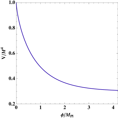
Figure 1: The potential (58) versus the field $\phi$ for $\mu=0.7$ and $n=0.7$. The potential has a finite value $V=M^{4}$ at $\phi=0$, but its derivatives diverge ($|V_{,\phi}|\to\infty$ and $V_{,\phi\phi}\to\infty$) as $\phi\to 0$.

Now we would like to consider a runaway positive potential in the Einstein frame. One example is

$$V(\phi)=M^{4}[1-\mu(1-e^{-\phi/M_{\rm pl}})^{n}]\,,$$ (58)

where $0<\mu<1$ and $0<n<1$. This potential behaves as $V(\phi)\simeq M^{4}[1-\mu(\phi/M_{\rm pl})^{n}]$ for $\phi\ll M_{\rm pl}$ and approaches $V(\phi)\to M^{4}(1-\mu)$ in the limit $\phi\gg M_{\rm pl}$ (see Fig. 1). For the potential (58) we obtain

$$\Gamma-1=\frac{1-nx-\mu(1-x)^{n}}{n\mu x(1-x)^{n}}\,,\qquad x\equiv e^{-\phi/M_{\rm pl}}\,.$$ (59)

One can easily show that the r.h.s. is positive under the conditions $0<\mu<1,0<n<1$, so that $\Gamma>1$. In both limits $\phi\to 0$ and $\phi\to\infty$ one has $\Gamma\to+\infty$. Since $\Gamma$ has a minimum at a finite field value, the condition $\Gamma\gg 1$ is not necessarily satisfied today (unlike the potential (56)).

Unless $\mu$ is very close to 1 the potential energy today is roughly of the order of $M^{4}$, i.e. $f(\phi_{0})\approx 1$. From Eq. (44) it then follows that

$$n\mu(1-x_{0})^{n-1}x_{0}\simeq Q\,,$$ (60)

where $x_{0}\equiv e^{-\phi_{0}/M_{\rm pl}}$. If $\phi_{0}\ll M_{\rm pl}$, we have that $\phi_{0}/M_{\rm pl}\simeq(n\mu)^{1/(1-n)}$. From Eq. (43) we obtain

$$n\mu(1-x_{B})^{n-1}x_{B}\simeq 10^{5}Q\,,$$ (61)

where $x_{B}\equiv e^{-\phi_{B}/M_{\rm pl}}$. Under the condition $\phi_{B}\ll M_{\rm pl}$ we have $\phi_{B}/M_{\rm pl}\simeq(10^{-5}n\mu/Q)^{1/(1-n)}$ from Eq. (61). Then the LLR bound (41) corresponds to

$$n\cdot 10^{10-15n}<Q/\mu\,.$$ (62)

When $\mu=0.5$ and $\mu=0.05$ with $Q=1$, the constraint (62) gives $n\gtrsim 0.63$ and $n\gtrsim 0.56$ respectively.

IV.3 Statefinder analysis

The statefinder diagnostics introduced in Refs. Sahni1 ; Sahni2 can be a useful tool to distinguish dark energy models from the $\Lambda$CDM model. The statefinder parameters are defined by

$$r=\frac{\dddot{a}}{aH^{3}}\,,\qquad s=\frac{r-1}{3(q-1/2)}\,,$$ (63)

where $q\equiv-\ddot{a}/(aH^{2})$ is the deceleration parameter. Defining $h\equiv H^{2}$, it follows that

$$q=-1-\frac{h^{\prime}}{2h}\,,\qquad r=1+\frac{h^{\prime\prime}}{2h}+\frac{3h^{\prime}}{2h}\,,$$ (64)

where a prime represents a derivative with respect to $N=\ln a$.

In the radiation dominated epoch we have $h\propto e^{-4N}$, which gives $(r,s)\simeq(3,4/3)$. During the matter era $r$ approaches $1$, whereas $s$ blows up from positive to negative because of the divergence of the denominator in $s$ (i.e. $q=1/2$). For the chameleon potentials (56) and (58) the solutions finally approach the de Sitter fixed point characterized by $(r,s)=(1,0)$. Around the de Sitter point the solutions evolve along the instantaneous minima characterized by $(x_{1},x_{2},x_{3})=(\lambda/\sqrt{6},\sqrt{1-\lambda^{2}/6},0)$ with $h\propto V$. Using Eq. (22) as well, one has $h^{\prime}/h\simeq-\lambda^{2}$ and $h^{\prime\prime}/h\simeq(2\Gamma-1)\lambda^{4}$. Then the statefinder diagnostics around the de Sitter point can be estimated as

$$r\simeq 1+\left(\Gamma-\frac{1}{2}\right)\lambda^{4}-\frac{3}{2}\lambda^{2}\,,$$ (65)

$$s\simeq-\frac{(2\Gamma-1)\lambda^{4}-3\lambda^{2}}{3(3-\lambda^{2})}\,.$$ (66)

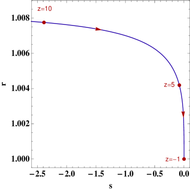
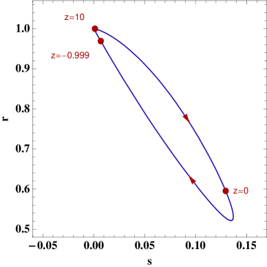
Figure 2: (Top): Evolution of the statefinders $r$ and $s$ for the potential (56) with $n=1$, $Q=1$ and $\mu=1$. The solutions approach the de Sitter point at $(r,s)=(1,0)$ from the region $r>1$ and $s<0$. (Bottom): Evolution of statefinders for the potential (58) with $n=0.7$, $Q=1$ and $\mu=0.7$. In this case the solutions approach the de Sitter point from the region $r<1$ and $s>0$.

Since $\lambda$ finally approaches 0, Eq. (22) implies that $\Gamma\lambda^{3}\to 0$ asymptotically. For the potential in which $\Gamma\gg 1$ holds today it can happen that $\Gamma\lambda^{4}\gg\lambda^{2}$, which gives $r\simeq 1+\Gamma\lambda^{4}>1$ and $s\simeq-2\Gamma\lambda^{4}/[3(3-\lambda^{2})]<0$ around the present epoch. In the upper panel of Fig. 2 we plot the evolution of the variables $r$ and $s$ for the potential (56) in the redshift regime $-1<z\equiv 1/a-1<10$. The statefinders evolve toward the de Sitter point characterized by $(r,s)=(1,0)$ from the regime $r>1$ and $s<0$. This behavior is different from quintessence with the power-law potential $V(\phi)=M^{4+n}\phi^{-n}$ ($n>0$) in which the statefinders are confined in the region $r<1$ and $s>0$ Sahni1 ; Sahni2 .

The potential (58) allows the possibility that $\Gamma$ is not much larger than 1 even at the present epoch. In the regime $\lambda^{2}\ll 1$ we then have $r\simeq 1-3\lambda^{2}/2<1$ and $s\simeq\lambda^{2}/3>0$. In fact we have numerically confirmed that the solutions enter this regime by today (see the lower panel of Fig. 2). Finally they approach the de Sitter point from the regime $r<1$ and $s>0$. Hence one can distinguish between chameleon potentials from the evolution of statefinders.

V Local gravity constraints on chameleon potentials

In this section we discuss a number of local gravity constraints on the chameleon potentials (56) and (58) in details. Together with the LLR bound (41) we use the constraint coming from 2006 Eöt-Wash experiments Kapner:2006si as well as the WMAP bound on the variation of the field-dependent mass.

V.1 The WMAP constraint on the variation of the particle mass

Due to the conformal coupling of the field $\phi$ to matter, any particle will acquire a $\phi$-dependent mass:

$$m(\phi)=m_{0}e^{Q\phi/M_{\rm pl}}\,,$$ (67)

where $m_{0}$ is a constant.

The WMAP data constrain any variation in $m(\phi)$, between now and the epoch of recombination to be $\lesssim 5\%$ at $2\sigma$ ($\lesssim 23\%$ at $4\sigma$) wmap_constraints . We then require that

$$\left|\frac{\Delta m(\phi)}{m}\right|=\left|e^{\frac{Q(\phi_{0}-\phi_{\rm rec})}{M_{\rm pl}}}-1\right|\lesssim 0.05\,,$$ (68)

where $\phi_{\rm rec}$ is the field value at the recombination epoch. If we assume that the chameleon follows the minimum since recombination then $\phi_{0}\gg\phi_{\rm rec}$, and the field in the cosmological background today must satisfy

$$Q\phi_{0}/M_{\rm pl}\lesssim 0.05\,.$$ (69)

This provides a constraint on the coupling $Q$ and the model parameters of chameleon potentials.

Note that the WMAP constraint is not a local gravity constraint. Nevertheless, it provides strong constraints on the potential (58) with natural parameters and is therefore considered in this section.

V.2 Constraints from the 2006 Eöt-Wash experiment

The 2006 Eöt-Wash experiment Kapner:2006si searched for deviations from the $1/r^{2}$ force law of gravity. The experiment used two parallel plates, the detector and attractor, which are separated by a (smallest) distance $d=55\mu$m. The plates have holes of different sizes bored into them, and the attractor is rotating with an angular velocity $\omega$. The rotation of the attractor gives rise to a torque on the detector, and the setup of the experiment is such that this torque vanishes for any force that falls off as $1/r^{2}$. In between the plates there is a $d_{s}=10\,\mu$m BeCu-sheet, which is for shielding the detector from electrostatic forces.

The chameleon force between two parallel plates, see e.g. Ref. Brax:2007vm , usually falls off faster than $1/r^{2}$, implying a strong signature on the experiment. However, if the matter-coupling is strong enough, the electrostatic shield will itself develop a thin-shell. When this happens, the effect of this shield is not only to shield electrostatic forces, but also to shield the chameleon force on the detector. This suppression is approximately given by a factor $\exp(-m_{s}d_{s})$, where $m_{s}$ is the mass inside the electrostatic shield. Hence the experiment cannot detect strongly coupled chameleons.

The behavior of chameleons in the Eöt-Wash experiment have been explained in Refs. Mota:2006fz ; Brax:2008hh ; Brax:2010kv . We calculate the Eöt-Wash constraints on our models numerically based on the prescription presented in Ref. Brax:2008hh .

V.3 Combined local gravity constraints

V.3.1 Potential $V(\phi)=M^{4}\exp[\mu(M/\phi)^{n}]$

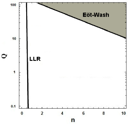
Figure 3: The combined local gravity constraints on the potential (56) with $\mu=1$ in the $(n,Q)$ plane. The shaded region corresponds to the allowed parameter space. The natural values of $Q$ and $n$ of the order of unity are excluded.

Let us first consider the inverse-power law potential (56) with $n>0$. From Eq. (12) the field value $\phi_{m}$ at the minimum of the effective potential $V_{\rm eff}$ satisfies

$$\left(\frac{M}{\phi_{m}}\right)^{n+1}=\frac{Q}{\mu n}\frac{M}{M_{\rm pl}}\frac{\rho_{m}e^{Q\phi_{m}/M_{\rm pl}}}{V(\phi_{m})}\,.$$ (70)

In this model the field is in the regime $M\ll\phi_{m}\ll M_{\rm pl}$ for the density $\rho_{m}$ we are interested in. Since $V(\phi_{m})$ can be approximated as $V(\phi_{m})\simeq M^{4}$, it follows that

$$\frac{\phi_{m}}{M}\simeq\left(\frac{Q}{\mu n}\frac{M}{M_{\rm pl}}\frac{\rho_{m}}{M^{4}}\right)^{-1/(n+1)}\,.$$ (71)

Using the LLR bound (41) with the homogeneous density $\rho_{m}\simeq 10^{-24}$ g/cm³ in our galaxy, we obtain the constraint

$$n\cdot 10^{10-15n}<Q/\mu\,.$$ (72)

The WMAP bound (69) gives

$$Q<\frac{M_{\rm pl}}{M}\left(\frac{0.05^{n+1}}{\mu n}\frac{\rho_{m}^{(0)}}{M^{4}}\right)^{1/n}\,,$$ (73)

where $\rho_{m}^{(0)}$ is the matter density today, with $\rho_{m}^{(0)}/M^{4}\approx\Omega_{m}^{*(0)}/\Omega_{\phi}^{(0)}\approx 1/3$. Since $M_{\rm pl}/M\approx 10^{30}$, this condition is well satisfied for $Q,n,\mu$ of the order of unity.

For the Eöt-Wash experiment, the chameleon torque on the detector was found numerically to be larger than the experimental bound when $Q,n,\mu$ are of the order of unity. Providing the electrostatic shield with a thin-shell, we require that $n\gg 1$, $Q\gg 1$ or $\mu\ll 1$ to satisfy the experimental bound.

In Fig. 3 we plot the region constrained by the bounds (72), (73), and the Eöt-Wash experiment for $\mu=1$. This shows that only the large coupling region with $Q\gg 1$ can be allowed for $n$ of the order of unity. A viable model can also be constructed by taking values of $\mu$ much smaller than 1. Note that the WMAP bound (73) is satisfied for the parameter regime shown in Fig. 3.

V.3.2 Potential $V(\phi)=M^{4}[1-\mu(1-e^{-\phi/M_{\rm pl}})^{n}]$

Let us proceed to another potential (58) with $0<n<1$. In the regions of high density where local gravity experiments are carried out, we have $\phi\ll M_{\rm pl}$ and hence $V(\phi)\simeq M^{4}[1-\mu(\phi/M_{\rm pl})^{n}]$. In this regime the effective potential $V_{\rm eff}$ has a minimum at

$$\phi_{m}=\left(\frac{Q}{\mu n}\frac{\rho_{m}}{M^{4}}\right)^{1/(n-1)}M_{\rm pl}\,.$$ (74)

Recall that the LLR bound was already derived in Eq. (62), which is the same as the constraint (72) of the previous potential.

Assuming that the chameleon is at the minimum of its effective potential in the cosmological background today, the WMAP bound (69) translates into

$$Q\gtrsim 0.05(60n\mu)^{1/n}\,,$$ (75)

where we have used $\rho_{m}^{(0)}/M^{4}\approx 1/3$ in Eq. (74). However, a full numerical simulation of the background evolution shows that this is not always the case. For a large range of parameters the chameleon has started to lag behind the minimum, which again leads to a weaker constraint.

The Eöt-Wash experiment provides the strongest constraints when $Q$ is of the order of unity for the potentials (51) and (56). This is not the case for the potential (58), because the electrostatic shield used in the experiment develops a thin-shell.

The mass inside the electrostatic shield is given by

$$m_{s}^{2}\simeq n(1-n)\mu\left(\frac{Q\rho_{s}}{\mu nM^{4}}\right)^{\frac{2-n}{1-n}}\frac{M^{4}}{M_{\rm pl}^{2}}\,.$$ (76)

Using $\rho_{s}\simeq 10$ g/cm³ and $d_{s}\simeq 10\,\mu$m we have

$$m_{s}d_{s}\simeq\sqrt{n(1-n)\mu}\left(\frac{Q}{\mu n}\right)^{\frac{2-n}{1-n}}10^{\frac{6-35n}{1-n}}\,.$$ (77)

Taking $Q$ and $\mu$ to be of the order of unity, we find $m_{s}d_{s}\gg 1$ as long as $n\gtrsim 0.2$. The suppression of the chameleon torque due to the presence of the electrostatic shield makes the chameleon invisible in the experiment.

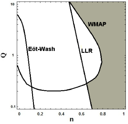
Figure 4: The combined local gravity constraints on the potential (58) with $\mu=0.5$ in the $(n,Q)$ plane. In this case the allowed parameter space (shaded region in the figure) is determined by the WMAP constraint and the LLR constraint.

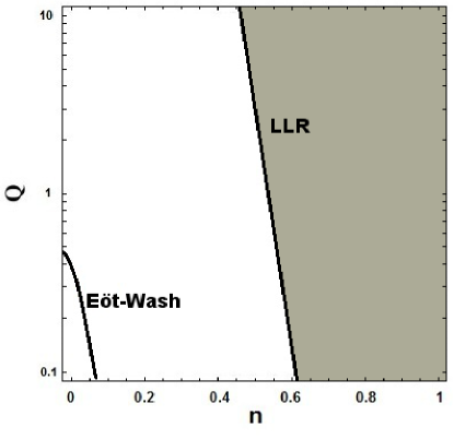
Figure 5: The combined local gravity constraints on the potential (58) with $\mu=0.05$. The allowed parameter space is determined by the LLR bound. The WMAP constraint is satisfied for the whole parameter space in the figure.

In Figs. 4 and 5 we plot the allowed regions constrained by the bounds (62), (75), and the Eöt-Wash experiments, for $\mu=0.5$ and $\mu=0.05$, respectively. When $\mu=0.5$ the WMAP constraint gives the tightest bound for $Q\gtrsim 0.2$, and the parameter space $Q\lesssim 1$ is viable for $n\gtrsim 0.7$. If we decrease the values of $\mu$ down to 0.05, then the WMAP bound is well satisfied for the parameter space shown in Fig. 5. Instead, the LLR experiment provides the tightest bound in such cases. When $\mu=0.05$, the region with $0.1\lesssim Q\lesssim 10$ and $n\gtrsim 0.6$ can be allowed. The coupling $Q$ as well as the parameter $n$ are not severely constrained for the potential (58).

VI Linear growth of matter perturbations

We now turn our attention to cosmological perturbations in chameleon cosmology. It is well-known that matter perturbations allow to discriminate between dark energy models where the gravitational interaction is modified on cosmic scales. We first review the general formalism and derive the equation for linear matter perturbations. We also introduce important quantities like the critical scale $\lambda_{c}$ below which modifications of gravity are felt and the growth index $\gamma(z,k)$, a powerful discriminative quantity for the study of the modified evolution of matter perturbations as was explained in the Introduction.

As we have seen in Sec. V, local gravity constraints impose very strong boundaries on the potential (56), forcing its parameters to take unnatural values. Moreover, for viable choices of parameters, we have verified that the linear perturbations behave in a manner similar to the $\Lambda$CDM model, as $\lambda_{c}$ is much smaller than the cosmic scales we are interested in. On the other hand we have shown that the model parameters of the potential (58) is not severely constrained. In Sec. VI.2 we will show that the potential (58) gives rise to some very interesting observational signatures.

VI.1 General formalism for cosmological perturbations

We consider scalar metric perturbations $\alpha$, $B$, $\psi$, and $\gamma$ around a flat FLRW background. The line-element describing such a perturbed Universe is given by Bardeen

$${{\rm d}}s^{2} = -(1+2\alpha){\rm d}t^{2}-2aB_{,i}{\rm d}t{\rm d}x^{i}$$ (78)

$$+a(t)^{2}\left[(1+2\psi)\delta_{ij}+2\gamma_{,i;j}\right]{\rm d}x^{i}{\rm d}x^{j}\,.$$

We decompose the field $\phi$ into the background and inhomogeneous parts: $\phi(t,{\bm{x}})=\tilde{\phi}(t)+\delta\phi(t,{\bm{x}})$. The energy-momentum tensors $T_{\mu\nu}^{(m)}$ of non-relativistic matter can be decomposed as

$${T^{0}_{0}}^{(m)}=-(\rho_{m}^{*}+\delta\rho_{m}^{*})\,,\qquad{T^{0}_{i}}^{(m)}=-\rho_{m}^{*}v_{,i}\,,$$ (79)

where $v$ is the peculiar velocity potential of non-relativistic matter. In the following, when we express background quantities, we drop the tilde for simplicity.

Let us consider the evolution of matter perturbations, $\delta_{m}\equiv\delta\rho_{m}^{*}/\rho_{m}^{*}$ in the comoving gauge ($v=0$). The quantity $\delta_{m}$ corresponds to the gauge-invariant quantity introduced in Refs. Bardeen ; S98 ; BEPS00 when expressed in the comoving gauge. In the Fourier space the first-order perturbation equations are given by Hwang:1991aj ; Amendolaper

$$\alpha=-Q\delta\phi/M_{\rm pl}\,,$$ (80)

$$\dot{\delta\rho^{*}_{m}}+3H\delta\rho^{*}_{m}-\rho^{*}_{m}\left(\kappa-3H\alpha\right)-Q(\rho^{*}_{m}\dot{\delta\phi}+\delta\rho^{*}_{m}\dot{\phi})/M_{\rm pl}=0\,,$$ (81)

$$\ddot{\delta\phi}+3H\dot{\delta\phi}+\left(V_{,\phi\phi}+\frac{k^{2}}{a^{2}}\right)\delta\phi+2\alpha V_{,\phi}-\dot{\phi}(\dot{\alpha}-3H\alpha+\kappa)+Q(2\alpha\rho_{m}^{*}+\delta\rho_{m}^{*})/M_{\rm pl}=0\,,$$ (82)

$$\dot{\kappa}+2H\kappa+3\dot{H}\alpha-\frac{k^{2}}{a^{2}}\alpha-\frac{1}{2M_{\rm pl}^{2}}\left(\delta\rho^{*}_{m}-4\alpha\dot{\phi}^{2}+4\dot{\phi}\dot{\delta\phi}-2V_{,\phi}\delta\phi\right)=0\,,$$ (83)

where $k$ is a comoving wavenumber and $\kappa\equiv 3(H\alpha-\dot{\psi})+(k^{2}/a)(B+a\dot{\gamma})$. From Eq. (81) it follows that

$$\kappa=\dot{\delta}_{m}-Q(\dot{\delta\phi}+3H\delta\phi)/M_{\rm pl}\,,$$ (84)

where we have used Eq. (80). Plugging Eq. (84) into Eqs. (82) and (83), we obtain

$$\ddot{\delta\phi}+\left(3H+2Q\frac{\dot{\phi}}{M_{\rm pl}}\right)\dot{\delta\phi}+\left(m_{\phi}^{2}+\frac{k^{2}}{a^{2}}-2Q\frac{V_{,\phi}}{M_{\rm pl}}-2Q^{2}\frac{\rho_{m}^{*}}{M_{\rm pl}^{2}}\right)\delta\phi+\frac{Q}{M_{\rm pl}}\rho_{m}^{*}\delta_{m}-\dot{\phi}\,\dot{\delta}_{m}=0\,,$$ (85)

$$\ddot{\delta}_{m}+\left(2H-Q\frac{\dot{\phi}}{M_{\rm pl}}\right)\dot{\delta}_{m}-\frac{\rho_{m}^{*}\delta_{m}}{2M_{\rm pl}^{2}}(1-2Q^{2})+\biggl{[}\frac{V_{,\phi}}{M_{\rm pl}^{2}}+\frac{Q}{M_{\rm pl}}\biggl{(}m_{\phi}^{2}+\frac{2k^{2}}{a^{2}}-6H^{2}-6\dot{H}-\frac{2\dot{\phi}^{2}}{M_{\rm pl}^{2}}$$

$$-2Q\frac{V_{,\phi}}{M_{\rm pl}}-2Q^{2}\frac{\rho_{m}^{*}}{M_{\rm pl}^{2}}\biggr{)}\biggr{]}\delta\phi+\frac{1}{M_{\rm pl}}\left(2Q^{2}\frac{\dot{\phi}}{M_{\rm pl}}-\frac{2\dot{\phi}}{M_{\rm pl}}-2QH\right)\dot{\delta\phi}=0\,,$$ (86)

where $m_{\phi}^{2}=V_{,\phi\phi}$ is the mass squared of the chameleon field.

As long as the field $\phi$ evolves slowly (“adiabatically”) along the instantaneous minima of the effective potential $V_{\rm eff}$, one can employ the quasi-static approximation on sub-horizon scales ($k\gg aH$) S98 ; BEPS00 ; quasi . This corresponds to the approximation under which the dominant terms in Eqs. (85) and (86) are those including $k^{2}/a^{2}$, $m_{\phi}$, and $\delta_{m}$, i.e.

$$\left(m_{\phi}^{2}+\frac{k^{2}}{a^{2}}\right)\delta\phi\simeq-\frac{Q}{M_{\rm pl}}\rho_{m}^{*}\delta_{m}\,,$$ (87)

$$\ddot{\delta}_{m}+2H\dot{\delta}_{m}-\frac{\rho_{m}^{*}\delta_{m}}{2M_{\rm pl}^{2}}(1-2Q^{2})$$

$$+\frac{Q}{M_{\rm pl}}\left(m_{\phi}^{2}+\frac{2k^{2}}{a^{2}}\right)\delta\phi\simeq 0\,,$$ (88)

where we have also used the approximation $\dot{\phi}/M_{\rm pl}\ll H$. Combining these equations, it follows that

$$\ddot{\delta}_{m}+2H\dot{\delta}_{m}-4\pi G_{{\rm eff}}\rho_{m}^{*}\delta_{m}\simeq 0\,,$$ (89)

where the effective gravitational coupling is given by

$$G_{{\rm eff}}=G\left(1+2Q^{2}\frac{k^{2}/a^{2}}{m_{\phi}^{2}+k^{2}/a^{2}}\right)\,.$$ (90)

An analogous modified equation was found in Refs. TUMTY ; BEPS00 ; Song , the crucial point being to elucidate the physical significance of $G_{\rm eff}$. We can understand the physical content of the modification of gravity by looking at the corresponding gravitational potential in real space. The gravitational potential (per unit mass) is of the type $V(r)=-(G/r)\left(1+2Q^{2}\,e^{-m_{\phi}r}\right)$ darkbook .

When we solve the full system of perturbations (86), we can, for some of our models, get a small discrepancy compared to (89). This can result in a non-negligible difference of up to around $5\%$ in the numerical calculation of the growth rate of matter perturbations. This arises mainly because the field $\phi$ does not move exactly along the minimum of the effective potential but is instead lagging a little behind it.

We see that in chameleon models $G_{\rm eff}$ is a scale-dependent as well as a time-dependent quantity. Clearly the scale-dependent driving force in Eq. (90) induces in turn a scale dependence in the growth of matter perturbations with two asymptotic regimes, i.e.

$$G_{\rm eff} =G(1+2Q^{2}) k/a \gg m_{\phi}~{}~{}{\rm or}~{}~{}\lambda\ll\lambda_{c}~{},$$ (91)

$$=G k/a \ll m_{\phi}~{}~{}{\rm or}~{}~{}\lambda\gg\lambda_{c}~{},$$ (92)

where we have introduced the physical wavelength $\lambda=(2\pi/k)a$. We have in particular $\lambda_{0}=2\pi/k$ today ($a=1$). The characteristic (physical) scale $\lambda_{c}$ is defined by

$$\lambda_{c}=2\pi/m_{\phi}\,.$$ (93)

On scales $\lambda\gg\lambda_{c}$ matter perturbations do not feel the fifth force during their growth. On the contrary, on scales much smaller than $\lambda_{c}$ they do feel its presence. During the matter dominance ($\Omega_{m}^{*}\simeq 1$) the solutions to Eq. (89) are given by

$$\delta_{m} \propto a^{[\sqrt{1+24(1+2Q^{2})}-1]/4} \lambda \ll\lambda_{c}\,,$$ (94)

$$\delta_{m} \propto a \lambda \gg\lambda_{c}\,.$$ (95)

Hence, in the regime $\lambda\ll\lambda_{c}$, the growth rate gets larger than that in standard General Relativity.

As mentioned earlier, a powerful way to describe the growth of perturbations is by introducing the function $\gamma(k,z)$ defined as follows

$$f=\Omega^{*}_{m}(z)^{\gamma(k,z)}~{},$$ (96)

where

$$f=\frac{{\rm d}\ln\delta_{m}}{{\rm d}\ln a}\,.$$ (97)

We remind the definition $\delta_{m}\equiv\delta\rho_{m}^{*}/\rho_{m}^{*}$. The quantity $\gamma$ can be time-dependent and also scale-dependent. It is known that a large class of dark energy models inside General Relativity yields a quasi-constant $\gamma$ with values close to that of the $\Lambda$CDM model, $\gamma\approx 0.55$ Linder ; PG07 . Therefore any significant deviation from this behavior would give rise to a characteristic signature for our chameleon models. Since $0<\Omega^{*}_{m}(z)<1$, smaller $\gamma$ implies a larger growth rate of matter perturbations.

As we have seen before, the chameleon mechanism is devised so that in high-density environments the mass of the scalar field is large relative to its value in low-density ones. During the cosmological evolution, the mass of the field will follow this behavior, which means that $\lambda_{c}$ will move from small to large values. In other words, $G_{\rm eff}$ will evolve from the regime (92) to the regime (91). This transition is scale-dependent, which is an important feature of the growth of matter perturbations in chameleon (and $f(R)$) models.

We consider the evolution of matter perturbations for the wavenumbers

$$0.01~{}h\,{\rm Mpc}^{-1}\lesssim k\lesssim 0.2~{}h\,{\rm Mpc}^{-1}\,,$$ (98)

where $h$ describes the uncertainty of the Hubble parameter $H_{0}$ today, i.e. $H_{0}=100\,h$ km sec^-1 Mpc^-1. The scales (98) range from the upper limit of observable scales in the linear regime of perturbations to the mildly non-linear regime (in which the linear approximation is still reasonable).

Depending on the value of $\lambda_{c}$ today (denoted as $\lambda_{c,0}$) and on its recent evolution, three possibilities can actually arise: (i) The model is hardly distinguishable from $\Lambda$CDM; (ii) The model is distinguishable from $\Lambda$CDM but shows no dispersion i.e. no scale-dependence. In this case low values of $\gamma_{0}$ will also yield large slopes $\gamma^{\prime}_{0}\equiv({\rm d}\gamma/{\rm d}z)(z=0)$, much larger than in $\Lambda$CDM; and finally (iii) The model is distinguishable from $\Lambda$CDM and shows some dispersion altogether. These three cases can be characterized using the quantity $\gamma_{0}\equiv\gamma(z=0)$. This classification is analogous to what was done for some viable $f(R)$ models Tsujikawa:2009ku and it can be defined as follows:

• (i) The region in parameter space for which $\gamma_{0}>0.53$ for all the scales described by (98). In this region $\gamma^{\prime}_{0}$ is small and $\gamma$ is nearly constant.

• (ii) The region where $\gamma_{0}$ is degenerate, i.e. assumes the same value for all the scales, with a value smaller than $0.5$. In this region $\gamma^{\prime}_{0}$ is large and there is a significant variation of $\gamma$.

• (iii) The region where $\gamma_{0}$ shows some dispersion, i.e. a scale-dependence. For low $\gamma_{0}$, $\gamma^{\prime}_{0}$ is large and we have significant changes of $\gamma$.

Models in the regions (ii) and (iii) can be clearly discriminated from $\Lambda$CDM. Some examples are shown in Figs. 6 and 7. We investigate below in more details the appearance of these characteristic signatures.

VI.2 Observational signatures in the growth of matter perturbations

The main question when looking at linear perturbations in chameleon models is the order of magnitude of the scale $\lambda_{c}$. If the chameleon mass $m_{\phi}$ is large such that $\lambda_{c}$ is less than the order of the galactic size, matter perturbations on the scales relevant to large scale structures do not feel the chameleon’s presence. This is actually the case for the inverse power exponential potential (56) with model parameters bounded by observational and local gravity constraints. Therefore, we will concentrate the analysis of the perturbations on the potential (58).

In the regime $\phi/M_{\rm pl}\ll 1$ one can employ the approximation $V(\phi)\simeq M^{4}[1-\mu(\phi/M_{\rm pl})^{n}]$. In fact this approximation is valid for most of the cosmological evolution by today. Then we obtain the field mass at the minimum of the effective potential $V_{\rm eff}(\phi)$:

$$m_{\phi}\simeq\frac{2\pi}{\lambda_{c,0}}e^{-\frac{3(2-n)}{2(1-n)}N}\,,$$ (99)

where $\lambda_{c,0}$ is the critical length today, given by

$$\lambda_{c,0}=\frac{2\pi}{\sqrt{\mu n(1-n)}}\frac{M_{\rm pl}}{M^{2}}\left(\frac{Q}{\mu n}\frac{\rho_{m}^{(0)}}{M^{4}}\right)^{-\frac{2-n}{2(1-n)}}\,.$$ (100)

Using the relation $\rho_{\rm DE}^{(0)}=3M_{\rm pl}^{2}H_{0}^{2}\Omega_{\rm DE}^{(0)}\simeq M^{4}$, we find that $\lambda_{c,0}$ is at most of the order of $H_{0}^{-1}$. If $Q=1$, $n=0.6$, $\mu=0.05$, and $\Omega_{\rm DE}^{(0)}=0.72$, for example, $\lambda_{c,0}\approx 0.4H_{0}^{-1}$. For the modes deep inside the Hubble radius today ($\lambda_{0}\ll H_{0}^{-1}$) the perturbations are affected by the modification of gravity.

Plugging Eq. (99) into Eq. (90), the effective gravitational coupling can be expressed in the form

$$G_{\rm eff}=G\left[1+\frac{2Q^{2}}{1+e^{-A(N-N_{c})}}\right]\,,$$ (101)

where

$$A = \frac{4-n}{1-n}\,,$$ (102)

$$N_{c} = \frac{2(1-n)}{4-n}\ln\left(\frac{\lambda_{0}}{\lambda_{c,0}}\right)\,.$$ (103)

Here $A$ and $N_{c}$ are the parameters describing respectively the steepness of transition from the inferior to the superior asymptote and the position of the half-amplitude value of the function [i.e. $G_{\rm eff}=G(1+Q^{2})$].

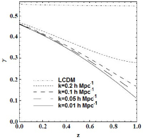
Figure 6: The evolution of the growth index $\gamma(z)$ versus the redshift $z$ in the model (58) with $n=0.8$, $\mu=0.5$ and $Q=1/\sqrt{6}$ for four different values of $k$. For these parameters, the model passes local gravity constraints. In this case the field is lagging behind the minimum, which means that the approximated equation (89) provides the results slightly different from this plot (by around 4% in the value of $\gamma_{0}$).

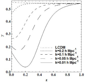
Figure 7: The evolution of $\gamma$ versus the redshift $z$ in the model (58) with $n=0.7$, $\mu=0.05$ and $Q=1$ for four different values of $k$. In this case the model passes local gravity constraints, too. Contrary to Fig. 6 we have a significant dispersion of $\gamma$, depending on the wavenumbers $k$.

The first interesting point to remark is that the steepness of transition depends exclusively on the value of $n$, with a step function as a limit when $n\rightarrow 1$ and a slower transition for $n\rightarrow 0$. Nonetheless, it must be remembered that this is so in the variable $N$. When converting back to the redshift $z$, the logarithm scale introduces a distortion, which means that the earlier a scale starts its transition, the slower this transition will be. In this sense, there is a scale-dependence to the steepness of the transition, even if it does not appear explicitly in Eq. (102).

If we want to get a better feel for the epoch of the transition, we can define the redshift $z_{c}={\rm e}^{-N_{c}}-1$. From Eq. (103) it follows that

$$z_{c}=\left(\frac{\lambda_{c,0}}{\lambda_{0}}\right)^{\frac{2(1-n)}{4-n}}-1\,.$$ (104)

As expected, the transition redshift is scale-dependent, with higher values for the smaller scales. Moreover, $z_{c}\rightarrow 0$ for all scales when $n\rightarrow 1$. Since this is also the limit at which the transition becomes a step function, we have thus an indication that a transition that happens very close to the present will necessarily be very steep. Another remark is that the transition happens in the past ($z_{c}>0$) for the scales $\lambda_{0}$ smaller than $\lambda_{c,0}$. Thus $\lambda_{c,0}$ is a good indication of the scale around which there will be a dispersion, as it marks the scale that will be exactly in the middle of the transition today.

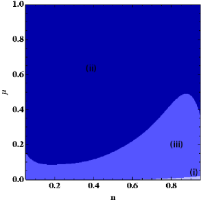
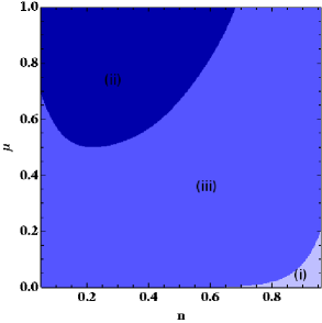
Figure 8: The regions (i), (ii) and (iii) in the ($n$,$\mu$) space for $Q=1/\sqrt{6}$ (top) and for $Q=1$ (bottom). In the region (i) all the modes have $\gamma_{0}>0.53$. In region (ii) $\gamma_{0}$ is degenerate with the value smaller than $0.5$, and finally (iii) shows the regime where $\gamma_{0}$ is dispersed. It is clear that, for both choices of $Q$, there are viable choices of parameters in which the deviation from the $\Lambda$CDM model is present.

If we write $z_{c}$ explicitly in terms of the parameters and constants of the model, we obtain

$$z_{c}=\left[\frac{(\mu n)^{\frac{1}{1-n}}}{1-n}\frac{k^{2}M_{\rm pl}^{2}}{M^{4}}\left(Q\frac{\rho_{m}^{(0)}}{M^{4}}\right)^{-\frac{2-n}{1-n}}\right]^{\frac{1-n}{4-n}}-1\,.$$ (105)

This shows that $z_{c}$ gets larger with increasing $\mu$ (as the deviation from the $\Lambda$CDM model is more significant) and/or decreasing $Q$. Although the transition occurs earlier for a weaker coupling $Q$, we need to take into account the fact that the growth rate in the regime $z<z_{c}$ is smaller for a weaker coupling.

Let us proceed to the numerical analysis of the growth of perturbations. In Fig. 6 we plot the evolution of the growth indices $\gamma$ for $Q=1/\sqrt{6}$, $n=0.8$ and $\mu=0.5$ for a number of different wavenumbers within the range specified by Eq. (98). Note that these parameters satisfy the local gravity constraints discussed in Sec. V, see Fig. 4. At the present epoch these modes are in the regime (ii), with very similar growth indices today ($\gamma_{0}\simeq 0.46$). As estimated by Eq. (105) the transition redshift $z_{c}$ is larger than the order of 1 for $k\gtrsim 0.05\,h$ Mpc^-1, e.g. $z_{c}=2.3$ for $k=0.1\,h$ Mpc^-1. The degenerate behavior similar to that shown in Fig. 6 has been also found in some $f(R)$ models GMP08 ; Tsujikawa:2009ku . Numerically we have verified that values of $\gamma_{0}$ in this case are slightly higher than those expected in the asymptotic regime ($\lambda\ll\lambda_{c}$). This discrepancy comes from the fact that the chameleon field is lagging behind the minimum of the potential for this choice of parameters. As a result, we need to solve the full perturbation equations (85) and (86) instead of the approximated equation (89). Our numerical results show that there can be a discrepancy of up to a few percent in the growth rate calculated with the two different methods.

Another choice of parameters, which are compatible with local gravity constraints, is made in Fig. 7, where we see the evolution of the growth indices $\gamma$ for $Q=1$, $n=0.7$ and $\mu=0.05$. The behavior of the growth indices is very different from the one shown in Fig. 6. Clearly this corresponds to the regime (iii), in which $\gamma_{0}$ is dispersed with respect to the wavenumbers $k$. The reason for the dispersion is that the transition to the regime $\lambda\ll\lambda_{c}$ occurs on lower redshifts than in the case shown in Fig. 6.

In Fig. 8 we illustrate three different regimes in the $(n,\mu)$ plane for the couplings $Q=1/\sqrt{6}$ and $Q=1$. For the model parameters close to $(n,\mu)=(1,0)$, the perturbations behave similarly to those in the $\Lambda$CDM model [i.e., in the region (i)]. Figure 8 shows that the limits imposed by the constraints derived in Sec. V, although strong, allow the large parameter space for the existence of an enhanced growth of matter perturbations and for the presence of the dispersion of $\gamma_{0}$. Finally we note that the large variation of $\gamma$ in the regime $z\lesssim 1$ seen in Figs. 6 and 7 will also enable us to distinguish the chameleon models from the $\Lambda$CDM model.

VII Summary and Conclusions

In this paper we have studied observational signatures of a chameleon scalar field coupled to non-relativistic matter. If the chameleon field is responsible for the late-time cosmic acceleration, the field potentials need to be consistent with the small energy scale of dark energy as well as local gravity constraints. We showed that the inverse power potential cannot satisfy both cosmological and local gravity constraints. In general, we require that the chameleon potentials are of the form $V(\phi)=M^{4}[1+f(\phi)]$, where the function $f(\phi)$ is smaller than 1 today and $M$ is a mass that corresponds to the dark energy scale ($M\sim 10^{-12}$ GeV).

The potential $V(\phi)=M^{4}\exp[\mu(M/\phi)^{n}]$ is one of those viable candidates. However we showed that the allowed model parameter space is tightly constrained by the 2006 Eöt-Wash experiment. As we see in Fig. 3, the natural parameters with $n$ and $Q$ of the order of unity are excluded for $\mu=1$. Unless we choose unnatural values of $\mu$ smaller than $10^{-5}$, this potential is incompatible with local gravity constraints for $\{n,Q\}={\cal O}(1)$.

On the other hand, the novel chameleon potential $V(\phi)=M^{4}[1-\mu(1-e^{-\phi/M_{\rm pl}})^{n}]$, which has the asymptotic form $V(\phi)\simeq M^{4}[1-\mu(\phi/M_{\rm pl})^{n}]$ in the regime $\phi\ll M_{\rm pl}$, can be consistent with a number of local gravity experiments as well as cosmological constraints. In fact this case covers the viable potentials of $f(R)$ dark energy models in the Einstein frame. The allowed parameter regions in the $(n,Q)$ plane are illustrated in Figs. 4 and 5 for $\mu=0.5$ and $\mu=0.05$. This potential is viable for natural model parameters and for the coupling $Q$ of the order of unity.

In order to distinguish the chameleon models from the $\Lambda$CDM model at the background level, we discussed the evolution of the statefinders $(r,s)$ defined in Eq. (63). Unlike the $\Lambda$CDM model in which $r$ and $s$ are constant ($r=1$, $s=0$) the statefinders exhibit a peculiar evolution, as plotted in Fig. 2. For the potential $V(\phi)=M^{4}[1-\mu(1-e^{-\phi/M_{\rm pl}})^{n}]$ we found that $r<1$ and $s>0$ around the present epoch, but the solutions approach the de Sitter point $(r,s)=(1,0)$ in future. The upcoming observations of SN Ia may discriminate such an evolution from other dark energy models.

We have also studied the growth of matter perturbations for the chameleon potential $V(\phi)=M^{4}[1-\mu(1-e^{-\phi/M_{\rm pl}})^{n}]$. The presence of a fifth force between the field and non-relativistic matter (dark matter/baryons) modifies the equation of matter perturbations, provided that the field mass $m_{\phi}$ is smaller than the physical wavenumber $k/a$, or $\lambda<\lambda_{c}$. Cosmologically the field is heavy in the past (i.e. for large density), but the mass $m_{\phi}$ decreases by today (typically of the order of $H_{0}$) in order to realize the late-time cosmic acceleration. Then the transition from the regime $k/a<m_{\phi}$ ($\lambda>\lambda_{c}$) to the regime $k/a>m_{\phi}$ ($\lambda<\lambda_{c}$) can occur at the redshift $z_{c}$ given in Eq. (105). For the perturbations on smaller scales (i.e. larger $k$) the critical redshift $z_{c}$ tends to be larger.

For the model parameters and the coupling $Q$ bounded by a number of experimental and cosmological constraints, we have studied the evolution of the growth index $\gamma$ of matter perturbations. Apart from the “General relativistic regime” in which two parameters $n$ and $\mu$ of the potential (58) are close to $(n,\mu)=(1,0)$, we found that the values of $\gamma$ today exhibit either dispersion with respect to the wavenumbers $k$ (region (iii) in Fig. 8) or no dispersion, however with $\gamma_{0}$ smaller than 0.5 (region (ii) in Fig. 8). Both cases can be distinguished from the $\Lambda$CDM model (where $\gamma\simeq 0.55$). Moreover, as seen in Figs. 6 and 7, the variation of $\gamma$ on low redshifts is significant.

From observations of galaxy clustering we have not yet obtained the accurate evolution of $\gamma$. This is linked to the fact that all probes of clustering are plagued by a bias problem. However upcoming galaxy surveys may pin down the matter power spectrum to exquisite accuracy, together with a better understanding of bias. In order to confirm or rule out models like ours, one must also address the observability of $\gamma$ both as a function of $z$ and $k$. We hope that future observations will provide an exciting possibility to detect the fifth force induced by the chameleon scalar field.

References

- (1) V. Sahni and A. A. Starobinsky, Int. J. Mod. Phys. D 9, 373 (2000); S. M. Carroll, Living Rev. Rel. 4, 1 (2001); T. Padmanabhan, Phys. Rept. 380, 235 (2003); P. J. E. Peebles and B. Ratra, Rev. Mod. Phys. 75, 559 (2003); E. J. Copeland, M. Sami and S. Tsujikawa, Int. J. Mod. Phys. D 15, 1753 (2006); A. De Felice and S. Tsujikawa, Living Rev. Rel. 13, 3 (2010); P. Brax, arXiv:0912.3610 [astro-ph.CO]; S. Tsujikawa, arXiv:1004.1493 [astro-ph.CO].
- (2) S. Weinberg, Rev. Mod. Phys. 61, 1 (1989).
- (3) Y. Fujii, Phys. Rev. D 26, 2580 (1982); L. H. Ford, Phys. Rev. D 35, 2339 (1987); C. Wetterich, Nucl. Phys B. 302, 668 (1988); B. Ratra and J. Peebles, Phys. Rev D 37, 321 (1988); T. Chiba, N. Sugiyama and T. Nakamura, Mon. Not. Roy. Astron. Soc. 289, L5 (1997); R. R. Caldwell, R. Dave and P. J. Steinhardt, Phys. Rev. Lett. 80, 1582 (1998).
- (4) S. M. Carroll, Phys. Rev. Lett. 81, 3067 (1998).
- (5) M. Gasperini and G. Veneziano, Phys. Rept. 373, 1 (2003).
- (6) M. Gasperini, F. Piazza and G. Veneziano, Phys. Rev. D 65, 023508 (2002); T. Damour, F. Piazza and G. Veneziano, Phys. Rev. Lett. 89, 081601 (2002).
- (7) J. Khoury and A. Weltman, Phys. Rev. Lett. 93, 171104 (2004).
- (8) J. Khoury and A. Weltman, Phys. Rev. D 69 (2004) 044026.
- (9) I. Navarro and K. Van Acoleyen, JCAP 0702, 022 (2007); T. Faulkner, M. Tegmark, E. F. Bunn and Y. Mao, Phys. Rev. D 76, 063505 (2007).
- (10) S. Capozziello and S. Tsujikawa, Phys. Rev. D 77, 107501 (2008).
- (11) S. Tsujikawa, K. Uddin, S. Mizuno, R. Tavakol and J. Yokoyama, Phys. Rev. D 77, 103009 (2008).
- (12) L. Amendola, R. Gannouji, D. Polarski and S. Tsujikawa, Phys. Rev. D 75, 083504 (2007); B. Li and J. D. Barrow, Phys. Rev. D 75, 084010 (2007); L. Amendola and S. Tsujikawa, Phys. Lett. B 660, 125 (2008); W. Hu and I. Sawicki, Phys. Rev. D 76, 064004 (2007); A. A. Starobinsky, JETP Lett. 86, 157 (2007); S. A. Appleby and R. A. Battye, Phys. Lett. B 654, 7 (2007); S. Tsujikawa, Phys. Rev. D 77, 023507 (2008); E. V. Linder, Phys. Rev. D 80, 123528 (2009).
- (13) A. A. Starobinsky, Phys. Lett. B 91, 99 (1980).
- (14) L. Amendola, Phys. Rev. D 62, 043511 (2000).
- (15) P. Brax, C. van de Bruck, A. C. Davis, J. Khoury and A. Weltman, Phys. Rev. D 70, 123518 (2004).
- (16) D. F. Mota and J. D. Barrow, Phys. Lett. B 581, 141 (2004).
- (17) D. F. Mota and D. J. Shaw, Phys. Rev. Lett. 97, 151102 (2006).
- (18) P. Brax, C. van de Bruck, A. C. Davis and A. M. Green, Phys. Lett. B 633, 441 (2006).
- (19) B. Feldman and A. E. Nelson, JHEP 0608, 002 (2006).
- (20) D. F. Mota and D. J. Shaw, Phys. Rev. D 75, 063501 (2007).
- (21) P. Brax, C. van de Bruck, A. C. Davis, D. F. Mota and D. J. Shaw, Phys. Rev. D 76, 085010 (2007).
- (22) P. Brax, C. van de Bruck and A. C. Davis, Phys. Rev. Lett. 99, 121103 (2007).
- (23) P. Brax and J. Martin, Phys. Lett. B 647, 320 (2007).
- (24) P. Brax, C. van de Bruck, A. C. Davis, D. F. Mota and D. J. Shaw, Phys. Rev. D 76, 124034 (2007).
- (25) A. E. Nelson and J. Walsh, Phys. Rev. D 77, 095006 (2008).
- (26) T. Tamaki and S. Tsujikawa, Phys. Rev. D 78, 084028 (2008).
- (27) P. Brax, C. van de Bruck, A. C. Davis and D. J. Shaw, Phys. Rev. D 78, 104021 (2008).
- (28) H. Gies, D. F. Mota and D. J. Shaw, Phys. Rev. D 77, 025016 (2008).
- (29) D. F. Mota, V. Pettorino, G. Robbers and C. Wetterich, Phys. Lett. B 663, 160 (2008).
- (30) A. C. Davis, C. A. O. Schelpe and D. J. Shaw, Phys. Rev. D 80, 064016 (2009).
- (31) A. S. Chou et al. [GammeV Collaboration], Phys. Rev. Lett. 102, 030402 (2009).
- (32) S. Tsujikawa, T. Tamaki and R. Tavakol, JCAP 0905, 020 (2009).
- (33) I. Thongkool, M. Sami, R. Gannouji and S. Jhingan, Phys. Rev. D 80, 043523 (2009).
- (34) P. Brax, C. Burrage, A. C. Davis, D. Seery and A. Weltman, arXiv:0911.1267 [hep-ph].
- (35) A. Upadhye, J. H. Steffen and A. Weltman, Phys. Rev. D 81, 015013 (2010).
- (36) P. Brax, C. van de Bruck, A. C. Davis, D. J. Shaw and D. Iannuzzi, arXiv:1003.1605 [quant-ph].
- (37) P. Brax, R. Rosenfeld and D. A. Steer, arXiv:1005.2051 [astro-ph.CO].
- (38) P. Brax, C. van de Bruck, D. F. Mota, N. J. Nunes and H. A. Winther, arXiv:1006.2796 [astro-ph.CO].
- (39) D. J. Kapner et al., Phys. Rev. Lett. 98, 021101 (2007).
- (40) For a review of experimental tests of the Equivalence Principle and General Relativity, see C. M. Will, Theory and Experiment in Gravitational Physics, 2nd Ed., (Basic Books/Perseus Group, New York, 1993); C. M. Will, Living Rev. Rel. 9, 3 (2005).
- (41) R. Nagata, T. Chiba and N. Sugiyama, Phys. Rev. D 69, 083512 (2004).
- (42) V. Sahni, T. D. Saini, A. A. Starobinsky and U. Alam, JETP Lett. 77, 201 (2003).
- (43) U. Alam, V. Sahni, T. D. Saini and A. A. Starobinsky, Mon. Not. Roy. Astron. Soc. 344, 1057 (2003).
- (44) L. M. Wang and P. J. Steinhardt, Astrophys. J. 508, 483 (1998).
- (45) E. V. Linder, Phys. Rev. D 72, 043529 (2005).
- (46) D. Polarski and R. Gannouji, Phys. Lett. B 660, 439 (2008).
- (47) R. Gannouji and D. Polarski, JCAP 0805, 018 (2008).
- (48) R. Gannouji, B. Moraes and D. Polarski, JCAP 0902, 034 (2009).
- (49) H. Motohashi, A. A. Starobinsky, J. Yokoyama, Prog. Theor. Phys. 123, 887 (2010).
- (50) T. Narikawa and K. Yamamoto, Phys. Rev. D 81, 043528 (2010).
- (51) U. Alam, V. Sahni and A. A. Starobinsky, Astrophys. J. 704, 1086 (2009).
- (52) J. H. He, B. Wang and Y. P. Jing, JCAP 0907, 030 (2009).
- (53) R. Gannouji, B. Moraes and D. Polarski, arXiv:0907.0393 [astro-ph.CO].
- (54) S. Tsujikawa, R. Gannouji, B. Moraes and D. Polarski, Phys. Rev. D 80, 084044 (2009).
- (55) R. Bean and M. Tangmatitham, Phys. Rev. D 81, 083534 (2010).
- (56) A. Cimatti et al., arXiv:0912.0914 [astro-ph.CO].
- (57) R. Gannouji, D. Polarski, A. Ranquet and A. A. Starobinsky, JCAP 0609, 016 (2006).
- (58) L. Amendola, M. Kunz and D. Sapone, JCAP 0804, 013 (2008); C. Di Porto and L. Amendola, Phys. Rev. D 77, 083508 (2008).
- (59) D. F. Mota, J. R. Kristiansen, T. Koivisto and N. E. Groeneboom, Mon. Not. Roy. Astron. Soc. 382, 793 (2007); T. Koivisto and D. F. Mota, JCAP 0806, 018 (2008).
- (60) S. Nesseris and L. Perivolaropoulos, Phys. Rev. D 77, 023504 (2008).
- (61) L. Knox, Y. S. Song and J. A. Tyson, Phys. Rev. D 74, 023512 (2006); Y. S. Song and K. Koyama, JCAP 0901, 048 (2009); Y. S. Song and O. Dore, JCAP 0903, 025 (2009).
- (62) D. F. Mota, D. J. Shaw and J. Silk, Astrophys. J. 675, 29 (2008); D. F. Mota, JCAP 0809, 006 (2008).
- (63) G. Esposito-Farèse and D. Polarski, Phys. Rev. D 63, 063504 (2001).
- (64) J. M. Bardeen, Phys. Rev. D 22, 1882 (1980).
- (65) A. A. Starobinsky, JETP Lett. 68, 757 (1998).
- (66) B. Boisseau, G. Esposito-Farese, D. Polarski and A. A. Starobinsky, Phys. Rev. Lett. 85, 2236 (2000).
- (67) J. c. Hwang, Astrophys. J. 375, 443 (1991).
- (68) L. Amendola, Mon. Not. Roy. Astron. Soc. 312, 521 (2000); L. Amendola, Phys. Rev. D 69, 103524 (2004); L. Amendola, S. Tsujikawa and M. Sami, Phys. Lett. B 632, 155 (2006).
- (69) S. Tsujikawa, Phys. Rev. D 76, 023514 (2007); S. Tsujikawa, K. Uddin and R. Tavakol, Phys. Rev. D 77, 043007 (2008); A. De Felice, S. Mukohyama and S. Tsujikawa, Phys. Rev. D 82, 023524 (2010).
- (70) Y. S. Song, L. Hollenstein, G. Caldera-Cabral and K. Koyama, JCAP 1004, 018 (2010).
- (71) L. Amendola and S. Tsujikawa, Dark energy–theory and observations, Cambridge University Press (2010).