Strong convergence of an explicit numerical method for SDEs with nonglobally Lipschitz continuous coefficients

Abstract

On the one hand, the explicit Euler scheme fails to converge strongly to the exact solution of a stochastic differential equation (SDE) with a superlinearly growing and globally one-sided Lipschitz continuous drift coefficient. On the other hand, the implicit Euler scheme is known to converge strongly to the exact solution of such an SDE. Implementations of the implicit Euler scheme, however, require additional computational effort. In this article we therefore propose an explicit and easily implementable numerical method for such an SDE and show that this method converges strongly with the standard order one-half to the exact solution of the SDE. Simulations reveal that this explicit strongly convergent numerical scheme is considerably faster than the implicit Euler scheme.

T1Supported in part by the Collaborative Research Centre 701 “Spectral Structures and Topological Methods in Mathematics” and by the research project “Numerical solutions of stochastic differential equations with nonglobally Lipschitz continuous coefficients” both funded by the German Research Foundation.

, and

1 Introduction and main result

The explicit Euler scheme (see, e.g., Kloeden and Platen kp92 , Maruyama m55 and Milstein m95 ) is most commonly used for approximating stochastic differential equations (SDEs) with globally Lipschitz continuous coefficients. Unfortunately, the explicit Euler scheme does not converge in the strong mean square sense to the exact solution of an SDE with a superlinearly growing and globally one-sided Lipschitz continuous drift coefficient. Even worse, Theorem 1 in hjk11 shows for such an SDE that the absolute moments of the explicit Euler approximations at a finite time point $T\in(0,\infty)$ diverge to infinity. The implicit Euler scheme is better than the explicit Euler scheme in that it converges strongly to the exact solution of such an SDE (see Higham, Mao and Stuart hms02 ). However, additional computational effort is required for its implementation. Therefore, we wish to identify explicit numerical methods which are strongly convergent even for SDEs with superlinearly growing coefficients. In this article we propose a “tamed” version of the explicit Euler scheme in which the drift term is modified such that it is uniformly bounded. Being almost identical to the explicit Euler method, this version is explicit and easy to implement. Now the benefit of this “tamed” Euler scheme is that it converges strongly to the exact solution in case of SDEs with superlinearly growing coefficients. More precisely, the main result of this article shows that this “tamed” Euler scheme converges strongly with the standard convergence order $\frac{1}{2}$ to the exact solution of the SDE if the drift coefficient function is globally one-sided Lipschitz continuous and has an at most polynomially growing derivative. The diffusion coefficient is assumed to be globally Lipschitz continuous here. Simulations confirm our theoretical results.

Throughout the whole article we assume that the following setting is fulfilled. Let $T\in(0,\infty)$ be a fixed real number, let $(\Omega,\mathcal{F},\mathbb{P})$ be a probability space with normal filtration $(\mathcal{F}_{t})_{t\in[0,T]}$, let $d,m\in\mathbb{N}:=\{1,2,\ldots\}$, let $W=(W^{(1)},\ldots,W^{(m)})\dvtx[0,T]\times\Omega\rightarrow\mathbb{R}^{m}$ be an $m$-dimensional standard $(\mathcal{F}_{t})_{t\in[0,T]}$-Brownian motion and let $\xi\dvtx\Omega\rightarrow\mathbb{R}^{d}$ be an $\mathcal{F}_{0}/\mathcal{B}(\mathbb{R}^{d})$-measurable mapping with $\mathbb{E}[\|\xi\|^{p}]<\infty$ for all $p\in[1,\infty)$. Here and below we use the notation $\|v\|:=(|v_{1}|^{2}+\cdots+|v_{k}|^{2})^{{1/2}}$, $\langle v,w\rangle:=v_{1}\cdot w_{1}+\cdots+v_{k}\cdot w_{k}$ for all $v=(v_{1},\ldots,v_{k})$, $w=(w_{1},\ldots,w_{k})\in\mathbb{R}^{k}$, $k\in\mathbb{N}$, and $\|A\|:={\sup_{v\in\mathbb{R}^{l},\|v\|\leq 1}}\|Av\|$ for all $A\in\mathbb{R}^{k\times l}$, $k,l\in\mathbb{N}$. Moreover, let $\mu\dvtx\mathbb{R}^{d}\rightarrow\mathbb{R}^{d}$ be a continuously differentiable and globally one-sided Lipschitz continuous function whose derivative grows at most polynomially and let $\sigma=(\sigma_{i,j})_{i\in\{1,2,\ldots,d\},j\in\{1,2,\ldots,m\}}\dvtx\mathbb{R}^{d}\rightarrow\mathbb{R}^{d\times m}$ be a globally Lipschitz continuous function. More formally, suppose that there is a real number $c\in(0,\infty)$ such that $\|\mu^{\prime}(x)\|\leq c(1+\|x\|^{c})$, $\|\sigma(x)-\sigma(y)\|\leq c\|x-y\|$ and $\langle x-y,\mu(x)-\mu(y)\rangle\leq c\|x-y\|^{2}$ for all $x,y\in\mathbb{R}^{d}$. Then consider the SDE

$$dX_{t}=\mu(X_{t})\,dt+\sigma(X_{t})\,dW_{t},\qquad X_{0}=\xi,$$ (1)

for $t\in[0,T]$. The drift coefficient $\mu$ is the infinitesimal mean of the process $X$ and the diffusion coefficient $\sigma$ is the infinitesimal standard deviation of the process $X$. Under the above assumptions, the SDE (1) is known to have a unique strong solution. More formally, there exists an adapted stochastic process $X\dvtx[0,T]\times\Omega\rightarrow\mathbb{R}^{d}$ with continuous sample paths fulfilling

$$X_{t}=\xi+\int_{0}^{t}\mu(X_{s})\,ds+\int_{0}^{t}\sigma(X_{s})\,dW_{s}$$ (2)

for all $t\in[0,T]$ $\mathbb{P}$-a.s. We refer to Theorem 2 in Alyushina Alyushina1987 , Theorem 1 in Krylov Krylov1990 and Theorem 2.4.1 in Mao m97 for existence and uniqueness results for SDEs of the form (1).

The goal of this article is to solve the strong approximation problem (see, e.g., Kloeden and Platen kp92 , Section 9.3) of the SDE (1). More precisely, our aim is to find a numerical approximation $Y\dvtx\Omega\rightarrow\mathbb{R}^{d}$ which satisfies

$$(\mathbb{E}[\|X_{T}-Y\|^{2}])^{{1/2}}<\varepsilon$$ (3)

for a given precision $\varepsilon>0$ and which can be implemented with as little computational effort as possible. At this point let us comment on the importance of solving the strong approximation problem (3). A central motivation for studying strong approximations in the sense of (3) is Giles’ seminal paper g08b (see also Heinrich h98 ). There he introduces, in comparison to the classical Monte Carlo method, a very efficient, somehow accelerated Monte Carlo method for approximating moments or other expectations of functionals of the SDE solution via numerical schemes that converge strongly (see also Creutzig, Dereich, Müller-Gronbach and Ritter cdmr09 for an detailed comparison of the classical and the new “accelerated” Monte Carlo method). In view of this method, strong approximations of the exact solution of the SDE (1) in the sense of (3) yield very efficient approximations of expectations of functionals of the SDE solution and this is a central reason for developing strongly convergent numerical methods.

The simplest and most obvious idea to solve the strong approximation problem (3) is to apply the explicit Euler scheme to the SDE (1). More precisely, the explicit Euler method for the SDE (1) is given by mappings $\tilde{Y}_{n}^{N}\dvtx\Omega\rightarrow\mathbb{R}^{d}$, $n\in\{0,1,\ldots,N\}$, $N\in\mathbb{N}$, which satisfy $\tilde{Y}_{0}^{N}=\xi$ and

$$\tilde{Y}_{n+1}^{N}=\tilde{Y}_{n}^{N}+\frac{T}{N}\cdot\mu(\tilde{Y}_{n}^{N})+\sigma(\tilde{Y}_{n}^{N})\bigl{(}W_{{(n+1)T}/{N}}-W_{{nT}/{N}}\bigr{)}$$ (4)

for all $n\in\{0,1,\ldots,N-1\}$ and all $N\in\mathbb{N}$. In the literature (see, e.g., Theorem 10.2.2 in Kloeden and Platen kp92 , Theorem 1.1 in Milstein m95 or Theorem 3.1 in Yuan and Mao ym08 ) the convergence results for the explicit Euler scheme require the drift coefficient $\mu$ of the SDE (1) to be globally Lipschitz continuous or to grow at most linearly, which we have not assumed in our setting. As it turns out, the assumption of an at most linearly growing drift function is essentially necessary. More precisely, in the case $d=m=1$, it has recently been shown in hjk11 that the root mean square distance of the exact solution of the SDE (1) and of the explicit Euler approximation (4) diverges to infinity

$$\lim_{N\rightarrow\infty}(\mathbb{E}[\|X_{T}-\tilde{Y}_{N}^{N}\|^{2}])^{{1/2}}=\infty,$$ (5)

if the drift coefficient $\mu$ of the SDE (1) grows superlinearly, that is, if there are real numbers $\alpha,C\in(1,\infty)$ such that $|\mu(x)|\geq\frac{|x|^{\alpha}}{C}$ holds for all $|x|\geq C$. Thus the explicit Euler scheme (4) does not solve the strong approximation problem (3) of the SDE (1) in general. This is particularly unfortunate as SDEs with superlinearly growing coefficients are quite important in applications (see, e.g., BenguriaKac1981 , GinzburgLandau1950 , HutzenthalerWakolbinger2007 , KhasminskiiKlebaner2001 , Lythe1995 , Oettinger1996 , Schuss1980 ). We remark that in contrast to strong mean square convergence, pathwise convergence of the explicit Euler method (4) to the exact solution of the SDE (1) holds due to Gyöngy’s result g98b .

Another idea for solving the strong approximation problem (3) is to apply the implicit Euler scheme, a.k.a. backward Euler scheme (see Higham, Mao and Stuart hms02 ), to the SDE (1). The implicit Euler scheme for the SDE (1) is given by mappings $\hskip 1.0pt\tilde{\tilde{{Y}}}{}_{n}^{N}\dvtx\Omega\rightarrow\mathbb{R}^{d}$, $n\in\{0,1,\ldots,N\}$, $N\in\mathbb{N}$, which satisfy $\hskip 1.0pt\tilde{\tilde{{Y}}}{}_{0}^{N}=\xi$ and

$$\hskip 1.0pt\tilde{\tilde{{Y}}}{}_{n+1}^{N}=\hskip 1.0pt\tilde{\tilde{{Y}}}{}_{n}^{N}+\frac{T}{N}\cdot\mu(\hskip 1.0pt\tilde{\tilde{{Y}}}{}_{n+1}^{N})+\sigma(\hskip 1.0pt\tilde{\tilde{{Y}}}{}_{n}^{N})\bigl{(}W_{{(n+1)T}/{N}}-W_{{nT}/{N}}\bigr{)}$$ (6)

for all $n\in\{0,1,\ldots,N-1\}$ and all $N\in\mathbb{N}$. A solution of this implicit equation is guaranteed to exist and to be unique for $N\in\mathbb{N}$ large enough due to the globally one-sided Lipschitz continuity of $\mu$. In the same setting as in this article, Higham, Mao and Stuart showed in Theorem 5.3 in hms02 (see also h10 , hmps10 , h96 , lae08 , s10 , sm10a , sm10b , t02 and the references therein for more approximation results on implicit numerical methods for SDEs of the form (1)) that the implicit Euler scheme (6) converges with order $\frac{1}{2}$ to the exact solution of the SDE (1) in the root mean square sense, that is, they established the existence of a real number $C\in[0,\infty)$ such that

$$(\mathbb{E}[\|X_{T}-\hskip 1.0pt\tilde{\tilde{{Y}}}{}_{N}^{N}\|^{2}])^{{1/2}}\leq C\cdot N^{-{1}/{2}}$$ (7)

for all $N\in\mathbb{N}$. However, additional computational effort is required in order to implement (6) since the zero of a nonlinear equation has to be determined in each time step in (6).

To sum up, the explicit Euler scheme, on the one hand, is explicit and easily implemented but does, in general, not converge strongly to the exact solution of the SDE (1). The implicit Euler scheme, on the other hand, converges strongly to the exact solution of the SDE (1) but additional computational effort is required for its implementation. Therefore, we aim at a simple explicit numerical method which converges strongly to the exact solution of the SDE (1).

More formally, the following numerical method for approximating the solution of the SDE (1) is proposed here. Let $Y^{N}_{n}\dvtx\Omega\rightarrow\mathbb{R}^{d}$, $n\in\{0,1,\ldots,N\}$, $N\in\mathbb{N}$, be given by $Y^{N}_{0}=\xi$ and

$$Y_{n+1}^{N}=Y_{n}^{N}+\frac{{T}/{N}\cdot\mu(Y_{n}^{N})}{1+{T}/{N}\cdot\|\mu(Y_{n}^{N})\|}+\sigma(Y_{n}^{N})\bigl{(}W_{{(n+1)T}/{N}}-W_{{nT}/{N}}\bigr{)}$$ (8)

for all $n\in\{0,1,\ldots,N-1\}$ and all $N\in\mathbb{N}$. We refer to the numerical method (8) as a tamed Euler scheme. In this method the drift term $\frac{T}{N}\cdot\mu(Y_{n}^{N})$ is “tamed” by the factor $1/(1+\frac{T}{N}\cdot\|\mu(Y_{n}^{N})\|)$ for $n\in\{0,1,\ldots,N-1\}$ and $N\in\mathbb{N}$ in (8). Note that the norm of $\frac{T}{N}\cdot\mu(Y_{n}^{N})/(1+\frac{T}{N}\cdot\|\mu(Y_{n}^{N})\|)$ is bounded by $1$ for every $n\in\{0,1,\ldots,N-1\}$ and every $N\in\mathbb{N}$. This prevents the drift term from producing extraordinary large values. Additionally, the Taylor expansion of $\frac{T}{N}\cdot\mu(x)/(1+\frac{T}{N}\cdot\|\mu(x)\|)$ in $1/N$ for fixed $x\in\mathbb{R}$ is equal to the drift term $\frac{T}{N}\cdot\mu(x)$ plus terms of order $O(\frac{1}{N^{2}})$. More formally, we see that

$$Y_{n+1}^{N} = Y_{n}^{N}+\frac{T}{N}\cdot\mu(Y_{n}^{N})+\sigma(Y_{n}^{N})\bigl{(}W_{{(n+1)T}/{N}}-W_{{nT}/{N}}\bigr{)}$$

$${}-\biggl{(}\frac{T}{N}\biggr{)}^{2}\frac{\mu(Y_{n}^{N})\cdot\|\mu(Y_{n}^{N})\|}{1+{T}/{N}\cdot\|\mu(Y_{n}^{N})\|}$$

for all $n\in\{0,1,\ldots,N-1\}$ and all $N\in\mathbb{N}$. Thus the tamed Euler scheme (8) coincides with the explicit Euler method (4) up to terms of second order. Moreover, note that the tamed Euler scheme (8) can be simulated easily and the drift function $\mu$ needs to be evaluated only once in each iteration of (8). More precisely, having calculated $v:=\frac{T}{N}\cdot\mu(Y_{n}^{N})$, the drift term in (8) is then readily computed as $\frac{v}{1+\|v\|}$.

In order to formulate our convergence theorem for the tamed Euler method (8), we now introduce appropriate time continuous interpolations of the time discrete numerical approximations (8). More formally, let $\bar{Y}^{N}\dvtx[0,T]\times\Omega\rightarrow\mathbb{R}^{d}$, $N\in\mathbb{N}$, be a sequence of stochastic processes given by

$$\bar{Y}_{t}^{N}=Y_{n}^{N}+\frac{(t-{nT}/{N})\cdot\mu(Y_{n}^{N})}{1+{T}/{N}\cdot\|\mu(Y_{n}^{N})\|}+\sigma(Y_{n}^{N})(W_{t}-W_{{nT}/{N}})$$ (10)

for all $t\in[\frac{nT}{N},\frac{(n+1)T}{N}]$, $n\in\{0,1,\ldots,N-1\}$ and all $N\in\mathbb{N}$. Note that $\bar{Y}^{N}\dvtx\break[0$, $T]\times\Omega\rightarrow\mathbb{R}^{d}$ is an adapted stochastic process with continuous sample paths for every $N\in\mathbb{N}$. We are now ready to formulate the main result of this article.

Theorem 1.1 ((Main result))

Let the setting in this section be fulfilled. Then there exists a family $C_{p}\in[0,\infty)$, $p\in[1,\infty)$, of real numbers such that

$$\Bigl{(}\mathbb{E}\Bigl{[}{\sup_{t\in[0,T]}}\|X_{t}-\bar{Y}_{t}^{N}\|^{p}\Bigr{]}\Bigr{)}^{{1/p}}\leq C_{p}\cdot N^{-{1}/{2}}$$ (11)

for all $N\in\mathbb{N}$ and all $p\in[1,\infty)$. Here $X\dvtx[0,T]\times\Omega\rightarrow\mathbb{R}^{d}$ is the exact solution of the SDE (1) and $\bar{Y}^{N}\dvtx[0,T]\times\Omega\rightarrow\mathbb{R}^{d}$, $N\in\mathbb{N}$, are the time continuous interpolations (10) of the numerical approximations (8).

Inequality (11) shows that the time continuous tamed Euler approximations (10) converge in the strong $L^{p}$-sense with the supremum over the time interval $[0,T]$ inside the expectation to the exact solution of the SDE (1) with the standard convergence order $\frac{1}{2}$. For a lower bound of this type of convergence, the reader is referred to Theorem 3 in Müller-Gronbach m02 (see also Hofmann, Müller-Gronbach and Ritter hmr00a ).

While the detailed proof of Theorem 1.1 is postponed to Section 3, we now outline the central ideas in the proof of Theorem 1.1. The key difficulty in the proof of Theorem 1.1 is to establish that the tamed Euler approximations (8) satisfy the a priori moment bounds

$$\sup_{N\in\mathbb{N}}\sup_{n\in\{0,1,\ldots,N\}}\mathbb{E}[\|Y_{n}^{N}\|^{p}]<\infty$$ (12)

for all $p\in[1,\infty)$ (see Lemma 3.9 in Section 3 for the precise statement of this result). After having verified (12), Theorem 1.1 can, by exploiting (1), at least in the case $p=2$, be completed analogously to Theorem 4.4 in Higham, Mao and Stuart hms02 in which strong convergence of the explicit Euler method under the assumption of the moment bounds (12) has been established. However, note that, in contrast to the tamed Euler approximations (8), the explicit Euler approximations (4) fail to satisfy such moment bounds for SDEs with superlinearly growing coefficients (see (5) here and Theorem 1 in hjk11 for details). It is quite remarkable that changing the explicit Euler method by a second order term such as in (1) alters the behavior of the numerical method to such an extent.

Let us now go into details and sketch the central ideas of our proof of the moment bounds (12). The key idea here for showing (12) is to introduce appropriate stochastic processes that dominate the tamed Euler approximations (8) on appropriate subevents. More formally, let $D^{N}_{n}\dvtx\Omega\rightarrow[0,\infty)$, $n\in\{0,1,\ldots,N\}$, $N\in\mathbb{N}$, be defined by

$$D_{n}^{N} := (\lambda+\|\xi\|)\exp\Biggl{(}\lambda+\sup_{u\in\{0,1,\ldots,n\}}\sum_{k=u}^{n-1}\biggl{[}\lambda\|\Delta W_{k}^{N}\|^{2}$$

$$\hskip 66.0pt{}+\mathbh{1}_{\{{\Arrowvert Y_{k}^{N}\Arrowvert}\geq 1\}}\biggl{\langle}\frac{Y_{k}^{N}}{\|Y_{k}^{N}\|},\frac{\sigma(Y_{k}^{N})}{\|Y_{k}^{N}\|}\Delta W_{k}^{N}\biggr{\rangle}\biggr{]}\Biggr{)}$$

for all $n\in\{0,1,\ldots,N\}$ and all $N\in\mathbb{N}$ where $\lambda\in[1,\infty)$ and $\Delta W^{N}_{n}\dvtx\Omega\rightarrow\mathbb{R}^{m}$ are defined through $\lambda:=(1+2c+T+\|\mu(0)\|+\|\sigma(0)\|)^{4}$ and $\Delta W^{N}_{n}:=W_{{(n+1)T}/{N}}-W_{{nT}/{N}}$ for all $n\in\{0,1,\ldots,N-1\}$ and all $N\in\mathbb{N}$. We will refer to $D_{n}^{N}$, $n\in\{0,1,\ldots,N\}$, $N\in\mathbb{N}$, as dominating stochastic processes. Appropriate subevents are $\Omega_{n}^{N}$, $n\in\{0,1,\ldots,N\}$, $N\in\mathbb{N}$, given by

$$\Omega_{n}^{N} := \Bigl{\{}\omega\in\Omega\dvtx\sup_{k\in\{0,1,\ldots,n-1\}}D_{k}^{N}(\omega)\leq N^{{1}/({2c})},$$

$$\hskip 49.0pt{\sup_{k\in\{0,1,\ldots,n-1\}}}\|\Delta W_{k}^{N}(\omega)\|\leq 1\Bigr{\}}$$

for all $n\in\{0,1,\ldots,N\}$ and all $N\in\mathbb{N}$. The main step of our proof of the moment bounds (12) will be to establish the pathwise inequality

$$\mathbh{1}_{\Omega_{n}^{N}}\|Y_{n}^{N}\|\leq D_{n}^{N}$$ (15)

for all $n\in\{0,1,\ldots,N\}$ and all $N\in\mathbb{N}$ (see Lemma 3.1). The next step is then to obtain the moment bounds

$$\limsup_{N\rightarrow\infty}\mathbb{E}\Bigl{[}{\sup_{n\in\{0,1,\ldots,N\}}}|D_{n}^{N}|^{p}\Bigr{]}<\infty$$ (16)

for all $p\in[1,\infty)$ for the dominating stochastic processes (see Lemma 3.5). These follow nicely from Doob’s submartingale inequality (see, e.g., Theorem 11.2 in Klenke k08b ), from uniform boundedness of $\sigma(Y_{k}^{N})/\|Y_{k}^{N}\|$ on $\{\|Y_{k}^{N}\|\geq 1\}$ for all $k\in\{0,1,\ldots,N-1\}$, $N\in{\mathbb{N}}$ and from the fact that

$${\mathbb{E}}[\exp({\lambda}\|\Delta W_{k}^{N}\|^{2}+\langle v,\Delta W_{k}^{N}\rangle)]\leq\exp\biggl{(}\frac{2\lambda Tm}{N}+\frac{T\|v\|^{2}}{2N}\biggr{)}$$ (17)

for all $v\in{\mathbb{R}}^{m}$, $k\in\{0,1,\ldots,N-1\}$ and all $N\in\mathbb{N}$ with $N\geq 4T{\lambda}$ (see Lemmas 3.2–3.4 for details). Combining (15) and (16) shows that

$$\sup_{N\in\mathbb{N}}\sup_{n\in\{0,1,\ldots,N\}}\mathbb{E}[\mathbh{1}_{\Omega_{n}^{N}}\|Y_{n}^{N}\|^{p}]<\infty$$ (18)

for all $p\in[1,\infty)$. For proving (12), it thus remains to verify that

$$\sup_{N\in\mathbb{N}}\sup_{n\in\{0,1,\ldots,N\}}\mathbb{E}\bigl{[}\mathbh{1}_{(\Omega_{n}^{N})^{c}}\|Y_{n}^{N}\|^{p}\bigr{]}<\infty$$ (19)

for all $p\in[1,\infty)$. This can be achieved by exploiting that the probability of $(\Omega_{N}^{N})^{c}$ decays rapidly to zero as $N$ goes to infinity (see Lemma 3.6 for details) and by using that the norm $\|\frac{{T}/{N}\cdot\mu(Y_{n}^{N})}{1+{T}/{N}\cdot\|\mu(Y_{n}^{N})\|}\|\leq 1$ of the drift term in (8) is bounded by $1$ due to the taming factor $1/(1+\frac{T}{N}\cdot\|\mu(Y_{n}^{N})\|)$ for $n\in\{0,1,\ldots,N\}$ and $N\in\mathbb{N}$. This is, in fact, the only argument in our proof of Theorem 1.1 for which the taming factor in (8) is needed.

It remains to motivate the pathwise inequality (15). The following estimate might at least give an intuition for the case of globally Lipschitz continuous coefficients. Consider the tamed Euler scheme for a geometric Brownian motion [SDE (1) with $d=m=1$, $\mu(x)=0$ and $\sigma(x)=x$ for all $x\in{\mathbb{R}}$]. Using $1+x\leq e^{x}$ for $x\in{\mathbb{R}}$ yields that

$$\|Y_{n+1}^{N}\|^{2} = \|Y_{n}^{N}+Y_{n}^{N}\Delta W_{n}^{N}\|^{2}$$

$$= \|Y_{n}^{N}\|^{2}+\|Y_{n}^{N}\Delta W_{n}^{N}\|^{2}+2\langle Y_{n}^{N},Y_{n}^{N}\Delta W_{n}^{N}\rangle$$

$$= \|Y_{n}^{N}\|^{2}\biggl{(}1+\|\Delta W_{n}^{N}\|^{2}+2\biggl{\langle}\frac{Y_{n}^{N}}{\|Y_{n}^{N}\|},\frac{Y_{n}^{N}}{\|Y_{n}^{N}\|}\Delta W_{n}^{N}\biggr{\rangle}\biggr{)}$$

$$\leq \|Y_{n}^{N}\|^{2}\exp\biggl{(}\|\Delta W_{n}^{N}\|^{2}+2\biggl{\langle}\frac{Y_{n}^{N}}{\|Y_{n}^{N}\|},\frac{Y_{n}^{N}}{\|Y_{n}^{N}\|}\Delta W_{n}^{N}\biggr{\rangle}\biggr{)}$$

for all $n\in\{0,1,\ldots,N-1\}$ and all $N\in{\mathbb{N}}$. Iterating this inequality leads to an inequality such as (15). Of course, the case of superlinearly growing drift coefficients is more subtle and we refer to Section 3.1 for the detailed proof of inequality (15).

Having sketched the central ideas for the proof of our main result, we now compare Theorem 1.1 with some related results in the literature. A priori moment bounds of the form (12) for numerical methods for SDEs with nonglobally Lipschitz continuous coefficients have been intensively studied in the literature in recent years. Whereas the references hms02 , h96 , s10 , sm10b , sm10a , hmps10 deal with a priori moment bounds of the form (12) for implicit methods, references for explicit methods are infrequent. In particular, in 2002, Higham, Mao and Stuart formulated in hms02 , page 1060, the following open problem: “In general, it is not clear when such moment bounds can be expected to hold for explicit methods with ${f,g\in C^{1}}$” (drift and diffusion coefficients are denoted by $f$ and $g$ in hms02 instead of $\mu$ and $\sigma$ here). In 2010 an a priori moment bound for an explicit method has been proved in Bou-Rabee, Hairer and Vanden-Eijnden bhv10 . More precisely, in the setting of the Langevin equation (see Section 2 in bhv10 for the precise assumptions), Lemma 3.5 in bhv10 establishes exponential moment bounds for a version of the metropolis-adjusted Langevin algorithm (MALA) with reflection on the boundaries of certain compact sets. In this paper we concentrate on the explicit numerical method (8) in the setting of the SDE (1). To be more precise, in Lemma 3.9 in Section 3 below we show that the explicit method (8) fulfills (12) for all $p\in[1,\infty)$. Furthermore, we observe that one way of deriving the tamed Euler method (8) is to approximate the drift coefficent $\mu(v)$, $v\in\mathbb{R}^{d}$, in the SDE (1) by the modified drift coefficients $\frac{\mu(v)}{1+\lambda\|\mu(v)\|}$, $v\in\mathbb{R}^{d}$, for small $\lambda\in(0,\infty)$ and then to apply the explicit Euler method to these modified SDEs. Approximations of this type have been used in the literature in order to construct solutions of nonlinear parabolic unilateral problems (see, e.g., Palmeri Palmeri2000 , Section 3). Moreover, in the setting of the Langevin equation, Roberts and Tweedie suggested in 1996 a similar approximation step to (8) as a proposal for the Metropolis–Hastings method in order to sample from the invariant measure of the Langevin SDE (see rt96 , Subsection 1.4.3, (12)–(13)). The resulting Metropolis-adjusted method has been named Metropolis-adjusted Langevin truncated algorithm (MALTA). Finally, in 1998 a related class of numerical methods has been considered in Milstein, Platen and Schurz mps98 (see mps98 , (3.2)–(3.3)) in the case of globally Lipschitz continuous coefficients of the SDE. To sum up, in the general setting of the SDE (1), the tamed Euler method (8) is, to the best of our knowledge, the first explicit numerical method that has been shown to converge strongly to the exact solution of the SDE (1).

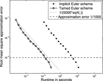
Figure 1: Root mean square approximation error $(\mathbb{E}\|X_{T}-\hskip 1.0pt\tilde{\tilde{{Y}}}{}_{N}^{N}\|^{2})^{{1}/{2}}$ of the exact solution of the SDE (21) and of the implicit Euler scheme (6) and root mean square approximation error $(\mathbb{E}\|X_{T}-Y_{N}^{N}\|^{2})^{{1}/{2}}$ of the exact solution of the SDE (21) and of the tamed Euler scheme (8) as function of the runtime when $N\in\{2^{4},2^{5},\ldots,2^{18}\}$.

We now compare simulations of the implicit Euler scheme (6) and of the tamed Euler scheme (8). For this we choose $T=d=m=1$, $\xi=1$, $\mu(x)=-x^{5}$ and $\sigma(x)=x$ for all $x\in\mathbb{R}$. The SDE (1) thus reads as

$$dX_{t}=-X_{t}^{5}\,dt+X_{t}\,dW_{t},\qquad X_{0}=1,$$ (21)

for $t\in[0,1]$. Suppose that the strong approximation problem (3) of the SDE (21) should be solved with the precision of say three decimals, that is, with precision $\varepsilon=\frac{1}{1000}$ in (3). Figure 1 depicts the root mean square approximation error $(\mathbb{E}\|X_{T}-\hskip 1.0pt\tilde{\tilde{{Y}}}{}_{N}^{N}\|^{2})^{{1}/{2}}$ of the exact solution of the SDE (21) and of the implicit Euler scheme (6) and the root mean square approximation error $(\mathbb{E}\|X_{T}-Y_{N}^{N}\|^{2})^{{1}/{2}}$ of the exact solution of the SDE (21) and of the tamed Euler scheme (8) as function of the runtime when $N\in\{2^{4},2^{5},\ldots,2^{18}\}$. The zero of the nonlinear equation that has to be determined in each time step of the implicit Euler scheme (6) is computed approximatively through the function $\mbox{fzero}(\ldots)$ in Matlab. It turns out that $\hskip 1.0pt\tilde{\tilde{{Y}}}{}_{2^{16}}^{2^{16}}$ in the case of the implicit Euler scheme (6) and that $Y_{2^{16}}^{2^{16}}$ in the case of the tamed Euler scheme (8) achieve the precision $\varepsilon=\frac{1}{1000}$ in (3). Following is our Matlab code for simulating the implicit Euler approximation $\hskip 1.0pt\tilde{\tilde{{Y}}}{}^{2^{16}}_{2^{16}}$ [see (6)] for the SDE (21):

Y = 1; N = 2^16;
for n=1:N
  v = Y + Y*randn/sqrt(N);
  Y = fzero(@(x)x + x^5/N - v, Y);
end

Next we specify our Matlab code for calculating the tamed Euler approximation $Y^{2^{16}}_{2^{16}}$ [see (8)] for the SDE (21):

Y = 1; N = 2^16;
for n=1:N
  v = -Y^5/N;
  Y = Y + v/(1+abs(v)) + Y*randn/sqrt(N);
end

The above Matlab code for calculating the implicit Euler approximation $\hskip 1.0pt\tilde{\tilde{{Y}}}{}^{2^{16}}_{2^{16}}$ requires, on our computer running at $2.33$ GHz, about $35.1$ seconds while the above Matlab code for calculating the tamed Euler approximation $Y^{2^{16}}_{2^{16}}$ requires about $0.0212$ seconds to be evaluated on the same computer. Thus, on the above computer, the tamed Euler scheme (8) for the SDE (21) is more than one thousand times faster than the implicit Euler scheme (6) in achieving a precision of three decimals in (3).

2 Further examples

In this section we present further simulations to illustrate the efficiency of the tamed Euler scheme (8). The next example is a one-dimensional stochastic Ginzburg–Landau equation with multiplicative noise (see, e.g., Kloeden and Platen kp92 , equation (4.52)). More formally, let $T=d=m=1$, $\xi=1$, $\mu(x)=x-x^{3}$ and $\sigma(x)=x$ for all $x\in\mathbb{R}$. The SDE (1) thus reads as

$$dX_{t}=(X_{t}-X_{t}^{3})\,dt+X_{t}\,dW_{t},\qquad X_{0}=1,$$ (22)

for $t\in[0,1]$. We now use the implicit Euler scheme (6) and the tamed Euler scheme (8) for approximating the SDE (22) and we assume again that the strong approximation problem (3) of the SDE (22) should be solved with the precision of three decimals, that is, with precision $\varepsilon=\frac{1}{1000}$ in (3). For implementing the implicit Euler scheme (6) in the case of the SDE (22), we observe that the drift coefficient of the SDE (22) is a one-dimensional polynomial of degree three. Roots of one-dimensional polynomials of degree three are known explicitly thanks to Cardano’s method. This explicit knowledge results in a faster implementation of the implicit Euler scheme (6) than using the Matlab function $\mbox{fzero}(\ldots)$. More precisely, if $p,q\in\mathbb{R}$ and if $q^{2}+(p/3)^{3}\geq 0$, then the only real-valued root of $x^{3}+px-2q=0$, $x\in\mathbb{R}$, is $x=(D+q)^{1/3}-(D-q)^{(1/3)}$ where $D=\sqrt{q^{2}+(p/3)^{3}}\in[0,\infty)$. Thus the implicit Euler scheme (6) for the SDE (22) becomes an explicit scheme and satisfies

$$\hskip 1.0pt\tilde{\tilde{{Y}}}{}_{n+1}^{N} = \bigl{(}\sqrt{(q^{N}_{n})^{2}+(N-1)^{3}/27}+q^{N}_{n}\bigr{)}^{{1}/{3}}$$

$${}-\bigl{(}\sqrt{(q^{N}_{n})^{2}+(N-1)^{3}/27}-q^{N}_{n}\bigr{)}^{{1}/{3}}$$

for all $n\in\{0,1,\ldots,N-1\}$ and all $N\in\mathbb{N}$ where $q^{N}_{n}\dvtx\Omega\rightarrow\mathbb{R}$ is defined by $q^{N}_{n}:=\hskip 1.0pt\tilde{\tilde{{Y}}}{}_{n}^{N}\cdot\frac{N}{2}\cdot(1+W_{{(n+1)T}/{N}}-W_{{nT}/{N}})$ for every $n\in\{0,1,\ldots,N-1\}$ and every $N\in\mathbb{N}$.

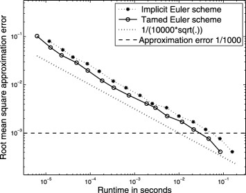
Figure 2: Root mean square approximation error $(\mathbb{E}\|X_{T}-\hskip 1.0pt\tilde{\tilde{{Y}}}{}_{N}^{N}\|^{2})^{{1}/{2}}$ of the exact solution of the SDE (22) and of the implicit Euler scheme (2) and root mean square approximation error $(\mathbb{E}\|X_{T}-Y_{N}^{N}\|^{2})^{{1}/{2}}$ of the exact solution of the SDE (22) and of the tamed Euler scheme (8) as function of the runtime when $N\in\{2^{4},2^{5},\ldots,2^{18}\}$.

Figure 2 displays the root mean square approximation error $(\mathbb{E}\|X_{T}-\hskip 1.0pt\tilde{\tilde{{Y}}}{}_{N}^{N}\|^{2})^{{1}/{2}}$ of the exact solution of the SDE (22) and of the implicit Euler scheme (2) and the root mean square approximation error $(\mathbb{E}\|X_{T}-Y_{N}^{N}\|^{2})^{{1}/{2}}$ of the exact solution of the SDE (22) and of the tamed Euler scheme (8) as function of the runtime when $N\in\{2^{4},2^{5},\ldots,2^{18}\}$. Comparing Figure 1 with Figure 2 confirms that using explicit knowledge of the roots of the involved implicit equation results in a much faster implementation of the implicit Euler scheme. The tamed Euler scheme, however, is still faster as its implementation does not require the arithmetical operations for calculating roots. More precisely, it turns out that $\hskip 1.0pt\tilde{\tilde{{Y}}}{}_{2^{17}}^{2^{17}}$ in the case of the implicit Euler scheme (2) and that $Y_{2^{17}}^{2^{17}}$ in the case of the tamed Euler scheme (8) achieve the desired precision $\varepsilon=\frac{1}{1000}$ in (3). Following is our Matlab code for simulating the implicit Euler approximation $\hskip 1.0pt\tilde{\tilde{{Y}}}{}^{2^{17}}_{2^{17}}$ for the SDE (22) [see (2)]:

Y = 1; N = 2^17; v = (N-1)^3/27;
for n=1:N
  q = Y*N*(1+randn/sqrt(N))/2;
  D = sqrt(q^2+v);
  Y = (D+q)^(1/3) - (D-q)^(1/3);
end

Next we specify our Matlab code for calculating the tamed Euler approximation $Y^{2^{17}}_{2^{17}}$ [see (8)] for the SDE (22):

Y = 1; N = 2^17;
for n=1:N
  v = (Y-Y^3)/N;
  Y = Y + v/(1+abs(v)) + Y*randn/sqrt(N);
end

The above Matlab code for calculating the implicit Euler approximation $\hskip 1.0pt\tilde{\tilde{{Y}}}{}^{2^{17}}_{2^{17}}$ requires, on our computer running at $2.33$ GHz, about $0.0836$ seconds while the above Matlab code for calculating the tamed Euler approximation $Y^{2^{17}}_{2^{17}}$ requires about $0.0467$ seconds to be evaluated on the same computer. Thus the tamed Euler scheme (8) is on our computer even in the case of the SDE (22), where the implicit Euler scheme can be computed explicitly, almost two times faster than the implicit Euler scheme (2) in achieving a precision of three decimals in (3).

Our last example is a multi-dimensional Langevin equation. More precisely, we consider the motion of a Brownian particle of unit mass in the $d$-dimensional potential $\frac{1}{4}\|x\|^{4}-\frac{1}{2}\|x\|^{2}$, $x\in\mathbb{R}^{d}$, where $d\in{\mathbb{N}}$. The corresponding force on the particle is then $x-\|x\|^{2}\cdot x$, $x\in{\mathbb{R}}^{d}$. More formally, let $T=1$, $m=d\in\mathbb{N}$, $\xi=(0,0,\ldots,0)$, $\mu(x)=x-\|x\|^{2}\cdot x$ and let $\sigma(x)=\mathrm{I}$ be the identity matrix for all $x\in\mathbb{R}^{d}$. Thus the SDE (1) reduces to the Langevin equation

$$dX_{t}=(X_{t}-\|X_{t}\|^{2}\cdot X_{t})\,dt+dW_{t},\qquad X_{0}=0,$$ (24)

for $t\in[0,1]$. Here $W\dvtx[0,1]\times\Omega\to{\mathbb{R}}^{d}$ is a $d$-dimensional standard Brownian motion.

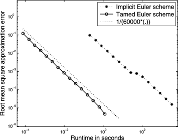
Figure 3: Root mean square approximation error $(\mathbb{E}\|X_{T}-\hskip 1.0pt\tilde{\tilde{{Y}}}{}_{N}^{N}\|^{2})^{{1}/{2}}$ of the exact solution of the SDE (24) with $d=10$ and of the implicit Euler scheme (6) and root mean square approximation error $(\mathbb{E}\|X_{T}-Y_{N}^{N}\|^{2})^{{1}/{2}}$ of the exact solution of the SDE (24) with $d=10$ and of the tamed Euler scheme (8) as function of the runtime when $N\in\{2^{4},2^{5},\ldots,2^{18}\}$.

Figure 3 displays the root mean square approximation error $(\mathbb{E}\|X_{T}-\hskip 1.0pt\tilde{\tilde{{Y}}}{}_{N}^{N}\|^{2})^{{1}/{2}}$ of the exact solution of the SDE (24) with $d=10$ and of the implicit Euler scheme (6) and the root mean square approximation error $(\mathbb{E}\|X_{T}-Y_{N}^{N}\|^{2})^{{1}/{2}}$ of the exact solution of the SDE (24) with $d=10$ and of the tamed Euler scheme (8) as function of the runtime when $N\in\{2^{4},2^{5},\ldots,2^{18}\}$. We see that both numerical approximations of the SDE (24) apparantly converge with rate $1$. This is presumably due to the additive noise in (24). Note that we used the Matlab function $\mbox{fsolve}(\ldots)$ in our implementation of the implicit Euler scheme (6) for the SDE (24) as the Matlab function $\mbox{fzero}(\ldots)$ used for the numerical simulations in Figure 1 is restricted to one dimension ($d=1$).

Some applications involve high-dimensional SDEs (see, e.g., Beskos and Stuart bs09 , Section 2.1). Then the above implementation of the implicit Euler method has an additional disadvantage. The Matlab command $\mbox{fsolve}(\ldots)$ uses (by default) the “trust-region-dogleg” algorithm which calculates Jacobian matrices. Thus the computational effort increases quadratically with the dimension $d\in\mathbb{N}$ for every fixed $N\in\mathbb{N}$. To visualize this we have plotted the runtime of the calculation of the implicit Euler approximation $\hskip 1.0pt\tilde{\tilde{{Y}}}{}_{128}^{128}$ of the SDE (24) as a function of the dimension $d\in\{10,20,30,\ldots,400\}$.

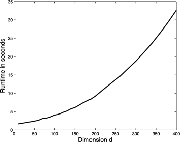
Figure 4: Runtime of the calculation of the implicit Euler approximation $\hskip 1.0pt\tilde{\tilde{{Y}}}{}_{128}^{128}$ of the SDE (24) as a function of the dimension $d\in\{10,20,30,\ldots,400\}$.

Figure 4 suggests a quadratic dependence of the runtime of the implicit Euler method on the dimension in case of the SDE (24). In contrast, the tamed Euler method is linear in the dimension (except that the evaluation of the coefficient functions might increase quadratically in the dimension).

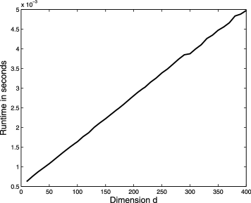
Figure 5: Runtime of the calculation of the tamed Euler approximation $Y_{128}^{128}$ of the SDE (24) as a function of the dimension $d\in\{10,20,30,\ldots,400\}$.

Figure 5 suggests a linear dependence of the runtime of the tamed Euler method on the dimension $d\in\{10,20,30,\ldots,400\}$ in case of the SDE (24).

3 Proof of Theorem 1.1

In order to simplify the notation introduced in Section 1, we introduce the mappings $\alpha^{N}_{n}\dvtx\Omega\rightarrow\mathbb{R}$ defined by

$$\alpha_{n}^{N}:=\mathbh{1}_{\{\|Y_{n}^{N}\|\geq 1\}}\biggl{\langle}\frac{Y_{n}^{N}}{\|Y_{n}^{N}\|},\frac{\sigma(Y_{n}^{N})}{\|Y_{n}^{N}\|}\Delta W_{n}^{N}\biggr{\rangle}$$ (25)

for all $n\in\{0,1,\ldots,N-1\}$ and all $N\in\mathbb{N}$. Using this notation, the dominating stochastic processes $D^{N}_{n}$, $n\in\{0,1,\ldots,N\}$, $N\in\mathbb{N}$, [see (1)] simplify to

$$D_{n}^{N}=(\lambda+\|\xi\|)\cdot\exp\Biggl{(}\lambda+\sup_{u\in\{0,1,\ldots,n\}}\sum_{k=u}^{n-1}[\lambda\|\Delta W_{k}^{N}\|^{2}+\alpha^{N}_{k}]\Biggr{)}$$

for all $n\in\{0,1,\ldots,N\}$ and all $N\in\mathbb{N}$. Moreover, we denote by $\vec{e}_{1}=(1,0,\ldots,\break 0)\in\mathbb{R}^{m}$, $\vec{e}_{2}=(0,1,0,\ldots,0)\in\mathbb{R}^{m},\ldots,\vec{e}_{m}=(0,\ldots,0,1)\in\mathbb{R}^{m}$ the unit vectors in the $\mathbb{R}^{m}$. Additionally, we use the mappings $\sigma_{i}\dvtx\mathbb{R}^{d}\rightarrow\mathbb{R}^{d}$, $i\in\{1,2,\ldots,\break m\}$, given by $\sigma_{i}(x)=(\sigma_{1,i}(x),\ldots,\sigma_{d,i}(x))=\sigma(x)\vec{e}_{i}$ for all $x\in\mathbb{R}^{d}$ and all $i\in\{1,2,\ldots,m\}$. The SDE (2) can thus be written as

$$X_{t}=\xi+\int_{0}^{t}\mu(X_{s})\,ds+\sum_{i=1}^{m}\int_{0}^{t}\sigma_{i}(X_{s})\,dW^{(i)}_{s}$$ (26)

for all $t\in[0,T]$ $\mathbb{P}$-a.s. Our proof of Theorem 1.1 relies on the following lemmas.

Lemma 3.1 ((Dominator lemma))

Let $Y_{n}^{N}\dvtx\Omega\to\mathbb{R}^{d}$, $D^{N}_{n}\dvtx\Omega\to[0,\infty)$ and $\Omega^{N}_{n}\in\mathcal{F}$ for $n\in\{0,1,\ldots,N\}$ and $N\in\mathbb{N}$ be given by (8), (1) and (1). Then we have that

$$\mathbh{1}_{\Omega_{n}^{N}}\|Y_{n}^{N}\|\leq D_{n}^{N}$$ (27)

for all $n\in\{0,1,\ldots,N\}$ and all $N\in{\mathbb{N}}$.

Lemma 3.2

Let $n\in\mathbb{N}$ and let $Z\dvtx\Omega\rightarrow\mathbb{R}^{n}$ be an $n$-dimensional standard normal random variable. Then we have that

$$\mathbb{E}[\exp(a\|Z\|^{2})]=(1-2a)^{-{n}/{2}}\leq e^{2an}$$ (28)

for all $a\in[0,\frac{1}{4}]$.

Lemma 3.3

We have that

$$\mathop{\sup_{N\in\mathbb{N},}}_{N\geq 4\lambda pT}\mathbb{E}\Biggl{[}\exp\Biggl{(}p\lambda\sum_{k=0}^{N-1}\|\Delta W_{k}^{N}\|^{2}\Biggr{)}\Biggr{]}<\infty$$ (29)

for all $p\in[1,\infty)$.

Lemma 3.4

Let $\alpha^{N}_{n}\dvtx\Omega\to\mathbb{R}$ for $n\in\{0,1,\ldots,N\}$ and $N\in\mathbb{N}$ be given by (25). Then we have that

$$\sup_{z\in\{-1,1\}}\sup_{N\in\mathbb{N}}\mathbb{E}\Biggl{[}\sup_{n\in\{0,1,\ldots,N\}}\exp\Biggl{(}pz\sum_{k=0}^{n-1}\alpha_{k}^{N}\Biggr{)}\Biggr{]}<\infty$$ (30)

for all $p\in[1,\infty)$.

Lemma 3.5 ((Uniformly bounded moments of the dominating stochastic processes))

Let $D_{n}^{N}\dvtx\Omega\to[0,\infty)$ for $n\in\{0,1,\ldots,N\}$ and $N\in\mathbb{N}$ be given by (1). Then we have that

$$\mathop{\sup_{N\in\mathbb{N},}}_{N\geq 8\lambda pT}\mathbb{E}\Bigl{[}{\sup_{n\in\{0,1,\ldots,N\}}}|D_{n}^{N}|^{p}\Bigr{]}<\infty$$ (31)

for all $p\in[1,\infty)$.

Lemma 3.6 ((Estimation of the probability of the complement of $\Omega^{N}_{N}$ for $N\in\mathbb{N}$))

Let $\Omega_{N}^{N}\in\mathcal{F}$ for $N\in\mathbb{N}$ be given by (1). Then we have that

$$\sup_{N\in{\mathbb{N}}}\bigl{(}N^{p}\cdot\mathbb{P}[(\Omega_{N}^{N})^{c}]\bigr{)}<\infty$$ (32)

for all $p\in[1,\infty)$.

Lemma 3.7 ((Time continuous Burkholder–Davis–Gundy type inequality))

Let $k\in{\mathbb{N}}$ and let $Z\dvtx[0,T]\times\Omega\to{\mathbb{R}}^{k\times m}$ be a predictable stochastic process satisfying $\mathbb{P}[\int_{0}^{T}\|Z_{s}\|^{2}\,ds<\infty]=1$. Then we obtain that

$$\qquad\biggl{\|}\sup_{s\in[0,t]}\biggl{\|}\int_{0}^{s}Z_{u}\,dW_{u}\biggr{\|}\biggr{\|}_{L^{p}(\Omega;{\mathbb{R}})}\leq p\Biggl{(}\int_{0}^{t}\sum_{i=1}^{m}\|Z_{s}\vec{e}_{i}\|_{L^{p}(\Omega,{\mathbb{R}}^{k})}^{2}\,ds\Biggr{)}^{{1}/{2}}$$ (33)

for all $t\in[0,T]$ and all $p\in[2,\infty)$.

Lemma 3.8 ((Time discrete Burkholder–Davis–Gundy type inequality))

Let $k\in{\mathbb{N}}$ and let $Z_{l}^{N}\dvtx\Omega\to{\mathbb{R}}^{k\times m}$, $l\in\{0,1,\ldots,N-1\}$, $N\in\mathbb{N}$, be a family of mappings such that $Z_{l}^{N}\dvtx\Omega\to{\mathbb{R}}^{k\times m}$ is $\mathcal{F}_{{lT}/{N}}/\mathcal{B}(\mathbb{R}^{k\times m})$-measurable for all $l\in\{0,1,\ldots,N-1\}$ and all $N\in{\mathbb{N}}$. Then we obtain that

$$\Biggl{\|}\sup_{j\in\{0,1,\ldots,n\}}\Biggl{\|}\sum_{l=0}^{j-1}Z_{l}^{N}\Delta W_{l}^{N}\Biggr{\|}\Biggr{\|}_{L^{p}(\Omega;{\mathbb{R}})}\leq p\Biggl{(}\sum_{l=0}^{n-1}\sum_{i=1}^{m}\|Z_{l}^{N}\vec{e}_{i}\|_{L^{p}(\Omega;{\mathbb{R}}^{k})}^{2}\frac{T}{N}\Biggr{)}^{{1}/{2}}$$ (34)

for all $n\in\{0,1,\ldots,N\}$, $N\in{\mathbb{N}}$ and all $p\in[2,\infty)$.

Lemma 3.9 ((Uniformly bounded moments of the tamed Euler approximations))

Let $Y_{n}^{N}\dvtx\Omega\to\mathbb{R}^{d}$ for $n\in\{0,1,\ldots,N\}$ and $N\in\mathbb{N}$ be given by (8). Then we have that

$$\sup_{N\in\mathbb{N}}\sup_{n\in\{0,1,\ldots,N\}}\mathbb{E}[\|Y_{n}^{N}\|^{p}]<\infty$$ (35)

for all $p\in[1,\infty)$.

Lemma 3.10

Let $Y_{n}^{N}\dvtx\Omega\to\mathbb{R}^{d}$ for $n\in\{0,1,\ldots,N\}$ and $N\in\mathbb{N}$ be given by (8). Then we have that

$$\sup_{N\in\mathbb{N}}\sup_{n\in\{0,1,\ldots,N\}}\mathbb{E}[\|\mu(Y_{n}^{N})\|^{p}]<\infty,\qquad\sup_{N\in\mathbb{N}}\sup_{n\in\{0,1,\ldots,N\}}\mathbb{E}[\|\sigma(Y_{n}^{N})\|^{p}]<\infty$$

for all $p\in[1,\infty)$.

The proofs of Lemmas 3.1–3.10 can be found in Sections 3.1–3.10. Using Lemmas 3.9 and 3.10, the proof of Theorem 1.1 is then completed in Section 3.11.

3.1 Proof of Lemma 3.1

First of all, note that $\|\Delta W_{n}^{N}\|\leq 1$ on $\Omega_{n+1}^{N}$ for all $n\in\{0,1,\ldots,N-1\}$ and all $N\in\mathbb{N}$. The global Lipschitz continuity of $\sigma$ and the polynomial growth bound on $\mu^{\prime}$ (see Section 1) therefore imply that

$$\|Y_{n+1}^{N}\| \leq \|Y_{n}^{N}\|+\frac{T}{N}\|\mu(Y_{n}^{N})\|+\|\sigma(Y_{n}^{N})\|\|\Delta W_{n}^{N}\|$$

$$\leq 1+T\|\mu(Y_{n}^{N})-\mu(0)\|+T\|\mu(0)\|$$

$${}+\|\sigma(Y_{n}^{N})-\sigma(0)\|+\|\sigma(0)\|$$

$$\leq 1+2Tc+T\|\mu(0)\|+c+\|\sigma(0)\|\leq\lambda$$

on $\Omega_{n+1}^{N}\cap\{\omega\in\Omega\dvtx\|Y^{N}_{n}(\omega)\|\leq 1\}$ for all $n\in\{0,1,\ldots,N-1\}$ and all $N\in\mathbb{N}$.

Moreover, the Cauchy–Schwarz inequality and the estimate $a\cdot b\leq\frac{a^{2}}{2}+\frac{b^{2}}{2}$ for all $a,b\in\mathbb{R}$ show that

$$\|Y_{n+1}^{N}\|^{2} = \biggl{\|}Y_{n}^{N}+\frac{({T}/{N})\mu(Y_{n}^{N})}{1+({T}/{N}){\Arrowvert\mu(Y_{n}^{N})\Arrowvert}}+\sigma(Y_{n}^{N})\Delta W_{n}^{N}\biggr{\|}^{2}$$

$$= \|Y_{n}^{N}\|^{2}+\frac{\|({T}/{N})\mu(Y_{n}^{N})\|^{2}}{(1+({T}/{N}){\Arrowvert\mu(Y_{n}^{N})\Arrowvert})^{2}}+\|\sigma(Y_{n}^{N})\Delta W_{n}^{N}\|^{2}$$

$${}+\frac{2\langle Y_{n}^{N},({T}/{N})\mu(Y_{n}^{N})\rangle}{1+({T}/{N}){\Arrowvert\mu(Y_{n}^{N})\Arrowvert}}+2\langle Y_{n}^{N},\sigma(Y_{n}^{N})\Delta W_{n}^{N}\rangle$$

$${}+\frac{2\langle({T}/{N})\mu(Y_{n}^{N}),\sigma(Y_{n}^{N})\Delta W_{n}^{N}\rangle}{1+({T}/{N}){\Arrowvert\mu(Y_{n}^{N})\Arrowvert}}$$

$$\leq \|Y_{n}^{N}\|^{2}+\frac{T^{2}}{N^{2}}\|\mu(Y_{n}^{N})\|^{2}+\|\sigma(Y_{n}^{N})\|^{2}\|\Delta W_{n}^{N}\|^{2}$$

$${}+\frac{({2T}/{N})\langle Y_{n}^{N},\mu(Y_{n}^{N})\rangle}{1+({T}/{N})\|\mu(Y_{n}^{N})\|}+2\langle Y_{n}^{N},\sigma(Y_{n}^{N})\Delta W_{n}^{N}\rangle$$

$${}+\frac{2T}{N}\|\mu(Y_{n}^{N})\|\|\sigma(Y_{n}^{N})\|\|\Delta W_{n}^{N}\|$$

$$\leq \|Y_{n}^{N}\|^{2}+\frac{2T^{2}}{N^{2}}\|\mu(Y_{n}^{N})\|^{2}+2\|\sigma(Y_{n}^{N})\|^{2}\|\Delta W_{n}^{N}\|^{2}$$

$${}+\frac{({2T}/{N})\langle Y_{n}^{N},\mu(Y_{n}^{N})\rangle}{1+({T}/{N})\|\mu(Y_{n}^{N})\|}+2\langle Y_{n}^{N},\sigma(Y_{n}^{N})\Delta W_{n}^{N}\rangle$$

on $\Omega$ for all $n\in\{0,1,\ldots,N-1\}$ and all $N\in\mathbb{N}$. Additionally, the global Lipschitz continuity of $\sigma$ (see Section 1) implies that

$$\|\sigma(x)\|^{2} \leq \bigl{(}\|\sigma(x)-\sigma(0)\|+\|\sigma(0)\|\bigr{)}^{2}$$

$$\leq \bigl{(}c\|x\|+\|\sigma(0)\|\bigr{)}^{2}\leq\bigl{(}c+\|\sigma(0)\|\bigr{)}^{2}\|x\|^{2}$$

$$\leq \lambda\|x\|^{2}$$

for all $x\in{\mathbb{R}}^{d}$ with ${\Arrowvert x\Arrowvert}\geq 1$ and the global one-sided Lipschitz continuity of $\mu$ (see Section 1) gives that

$$\langle x,\mu(x)\rangle = \langle x,\mu(x)-\mu(0)\rangle+\langle x,\mu(0)\rangle$$

$$\leq c\|x\|^{2}+\|x\|\|\mu(0)\|\leq\bigl{(}c+\|\mu(0)\|\bigr{)}\|x\|^{2}$$

$$\leq \sqrt{\lambda}\|x\|^{2}$$

for all $x\in{\mathbb{R}}^{d}$ with ${\Arrowvert x\Arrowvert}\geq 1$. Furthermore, the polynomial growth bound on $\mu^{\prime}$ (see Section 1) yields that

$$\|\mu(x)\|^{2} \leq \bigl{(}\|\mu(x)-\mu(0)\|+\|\mu(0)\|\bigr{)}^{2}$$

$$\leq \bigl{(}c(1+\|x\|^{c})\|x\|+\|\mu(0)\|\bigr{)}^{2}\leq\bigl{(}2c\|x\|^{(c+1)}+\|\mu(0)\|\bigr{)}^{2}$$

$$\leq \bigl{(}2c+\|\mu(0)\|\bigr{)}^{2}\|x\|^{2(c+1)}\leq N\sqrt{\lambda}\|x\|^{2}$$

for all $x\in{\mathbb{R}}^{d}$ with $1\leq{\Arrowvert x\Arrowvert}\leq N^{{1}/({2c})}$ and all $N\in\mathbb{N}$. Combining (3.1)–(3.1) and $T^{2}+T\leq\sqrt{\lambda}$ then gives that

$$\|Y_{n+1}^{N}\|^{2} \leq \|Y_{n}^{N}\|^{2}+\frac{2T^{2}\sqrt{\lambda}}{N}\|Y_{n}^{N}\|^{2}+2\lambda\|Y_{n}^{N}\|^{2}\|\Delta W_{n}^{N}\|^{2}$$

$${}+\frac{2T\sqrt{\lambda}}{N}\|Y^{N}_{n}\|^{2}+2\langle Y_{n}^{N},\sigma(Y_{n}^{N})\Delta W_{n}^{N}\rangle$$

$$= \|Y_{n}^{N}\|^{2}\biggl{(}1+\frac{2(T^{2}+T)\sqrt{\lambda}}{N}+2\lambda\|\Delta W_{n}^{N}\|^{2}+2\alpha^{N}_{n}\biggr{)}$$

$$\leq \|Y_{n}^{N}\|^{2}\exp\biggl{(}\frac{2\lambda}{N}+2\lambda\|\Delta W_{n}^{N}\|^{2}+2\alpha^{N}_{n}\biggr{)}$$

on $\{\omega\in\Omega\dvtx 1\leq\|Y^{N}_{n}(\omega)\|\leq N^{{1}/({2c})}\}$ for all $n\in\{0,1,\ldots,N-1\}$ and all $N\in\mathbb{N}$.

Additionally, we use the mappings $\tau^{N}_{l}\dvtx\Omega\rightarrow\{-1,0,1,\ldots,l-1\}$, $l\in\{0,1,\break\ldots,N\}$, $N\in\mathbb{N}$, given by

$$\tau_{l}^{N}(\omega):=\max\bigl{(}\{-1\}\cup\bigl{\{}n\in\{0,1,\ldots,l-1\}|\|Y_{n}^{N}(\omega)\|\leq 1\bigr{\}}\bigr{)}$$ (42)

for all $\omega\in\Omega$, $l\in\{0,1,\ldots,N\}$ and all $N\in\mathbb{N}$.

With the estimates (3.1) and (3.1) at hand, we now establish (27) by induction on $n\in\{0,1,\ldots,N\}$ where $N\in\mathbb{N}$ is fixed. The base case $n=0$ is trivial. Now let $l\in\{0,1,\ldots,N-1\}$ be arbitrary and assume that inequality (27) holds for all $n\in\{0,1,\ldots,l\}$. We then show inequality (27) for $n=l+1$. More formally, we now establish that

$$\|Y_{l+1}^{N}(\omega)\|\leq D_{l+1}^{N}(\omega)$$ (43)

for all $\omega\in\Omega^{N}_{l+1}$. To this end let $\omega\in\Omega_{l+1}^{N}$ be arbitrary. From the induction hypothesis and from $\omega\in\Omega_{l+1}^{N}\subseteq\Omega_{n+1}^{N}$ it follows that $\|Y_{n}^{N}(\omega)\|\leq D_{n}^{N}(\omega)\leq N^{{1}/({2c})}$ for all $n\in\{0,1,\ldots,l\}$. By definition (42) we therefore obtain that $1\leq\|Y_{n}^{N}(\omega)\|\leq N^{{1}/({2c})}$ for all $n\in\{\tau^{N}_{l+1}(\omega)+1,\tau^{N}_{l+1}(\omega)+2,\ldots,l\}$. Estimate (3.1) thus gives that

$$\|Y^{N}_{n+1}(\omega)\|\leq\|Y_{n}^{N}(\omega)\|\cdot\exp\biggl{(}\frac{\lambda}{N}+\lambda\|\Delta W_{n}^{N}\|^{2}+\alpha_{n}^{N}(\omega)\biggr{)}$$ (44)

for all $n\in\{\tau^{N}_{l+1}(\omega)+1,\tau^{N}_{l+1}(\omega)+2,\ldots,l\}$. Iterating (44) hence yields that

$$\|Y_{l+1}^{N}(\omega)\|$$

$$\quad\leq\|Y_{l}^{N}(\omega)\|\cdot\exp\biggl{(}\frac{\lambda}{N}+\lambda\|\Delta W_{l}^{N}(\omega)\|^{2}+\alpha_{l}^{N}(\omega)\biggr{)}$$

$$\quad\leq\cdots\leq\bigl{\|}Y_{\tau_{l+1}^{N}(\omega)+1}^{N}(\omega)\bigr{\|}\cdot\exp\Biggl{(}\sum_{n=\tau_{l+1}^{N}(\omega)+1}^{l}\biggl{(}\frac{\lambda}{N}+\lambda\|\Delta W_{n}^{N}(\omega)\|^{2}+\alpha_{n}^{N}(\omega)\biggr{)}\Biggr{)}$$

$$\quad\leq\bigl{\|}Y_{\tau_{l+1}^{N}(\omega)+1}^{N}(\omega)\bigr{\|}\cdot\exp\Biggl{(}\lambda+\sup_{u\in\{0,1,\ldots,l+1\}}\sum_{n=u}^{l}\bigl{(}\lambda\|\Delta W_{n}^{N}(\omega)\|^{2}+\alpha_{n}^{N}(\omega)\bigr{)}\Biggr{)}.$$

Estimate (3.1) therefore shows that

$$\|Y_{l+1}^{N}(\omega)\|$$

$$\qquad\leq\bigl{(}\lambda+\|\xi(\omega)\|\bigr{)}\cdot\exp\Biggl{(}\lambda+\sup_{u\in\{0,1,\ldots,l+1\}}\sum_{n=u}^{l}\bigl{(}\lambda\|\Delta W_{n}^{N}(\omega)\|^{2}+\alpha_{n}^{N}(\omega)\bigr{)}\Biggr{)}$$ (45)

$$\qquad=D^{N}_{l+1}(\omega).$$

This finishes the induction step and the proof.

3.2 Proof of Lemma 3.2

We establish (28) in the case $n=1$. The general case then follows from independence. For the case $n=1$ note that

$$\frac{1}{(1-x)}\leq e^{2x}$$ (46)

for all $x\in[0,\frac{1}{2}]$. Inequality (46) then shows that

$$\mathbb{E}[\exp(aZ^{2})] = \int_{\mathbb{R}}e^{ax^{2}}\frac{1}{\sqrt{2\pi}}e^{-{x^{2}}/{2}}\,dx=\int_{\mathbb{R}}\frac{1}{\sqrt{2\pi}}e^{{-x^{2}}/({2(1-2a)^{-1}})}\,dx$$

$$= \frac{1}{\sqrt{1-2a}}\leq e^{2a}$$

for all $a\in[0,\frac{1}{4}]$. This completes the proof of Lemma 3.2.

3.3 Proof of Lemma 3.3

The independence of the random variables $\Delta W_{k}^{N}$, $k\in\{0,1,\ldots,N-1\}$, and Lemma 3.2 show that

$$\mathbb{E}\Biggl{[}\exp\Biggl{(}\lambda p\sum_{k=0}^{N-1}\|\Delta W_{k}^{N}\|^{2}\Biggr{)}\Biggr{]} = \prod_{k=0}^{N-1}\mathbb{E}[\exp(\lambda p\|\Delta W_{k}^{N}\|^{2})]$$

$$= (\mathbb{E}[\exp(\lambda p\|W_{{T}/{N}}\|^{2})])^{N}$$

$$\leq \exp(2\lambda pTm)<\infty$$

for all $N\in\mathbb{N}\cap[4\lambda pT,\infty)$ and all $p\in[1,\infty)$. This completes the proof of Lemma 3.3.

3.4 Proof of Lemma 3.4

First of all, note that the time discrete stochastic process $z\sum_{k=0}^{n-1}\alpha_{k}^{N}$, $n\in\{0,1,\ldots,N\}$, is an $(\mathcal{F}_{{nT}/{N}})_{n\in\{0,1,\ldots,N\}}$-martingale for every $z\in\{-1,1\}$ and every $N\in\mathbb{N}$. In particular, we therefore obtain that the time discrete stochastic process $\exp(z\sum_{k=0}^{n-1}\alpha_{k}^{N})$, $n\in\{0,1,\ldots,N\}$, is a positive $(\mathcal{F}_{{nT}/{N}})_{n\in\{0,1,\ldots,N\}}$-submartingale for every $z\in\{-1,1\}$ and every $N\in\mathbb{N}$. Doob’s maximal inequality (see, e.g., Klenke k08b , Theorem 11.2) hence shows that

$$\Biggl{\|}\sup_{n\in\{0,1,\ldots,N\}}\exp\Biggl{(}z\sum_{k=0}^{n-1}\alpha_{k}^{N}\Biggr{)}\Biggr{\|}_{L^{p}(\Omega;\mathbb{R})}\leq\frac{p}{(p-1)}\Biggl{\|}\exp\Biggl{(}z\sum_{k=0}^{N-1}\alpha_{k}^{N}\Biggr{)}\Biggr{\|}_{L^{p}(\Omega;\mathbb{R})}$$ (48)

for all $N\in\mathbb{N}$, $p\in(1,\infty)$ and all $z\in\{-1,1\}$. Moreover, we have that

$$\mathbb{E}\biggl{[}\biggl{|}pz\mathbh{1}_{\{\|x\|\geq 1\}}\biggl{\langle}\frac{x}{\|x\|},\frac{\sigma(x)}{\|x\|}\Delta W_{k}^{N}\biggr{\rangle}\biggr{|}^{2}\biggr{]}$$

$$\qquad=\frac{p^{2}T}{N}\mathbh{1}_{\{\|x\|\geq 1\}}\frac{\|(\sigma(x))^{*}x\|^{2}}{\|x\|^{4}}\leq\frac{p^{2}T}{N}\mathbh{1}_{\{\|x\|\geq 1\}}\frac{\|(\sigma(x))^{*}\|^{2}}{\|x\|^{2}}$$

$$\qquad=\frac{p^{2}T}{N}\mathbh{1}_{\{\|x\|\geq 1\}}\frac{\|\sigma(x)\|^{2}}{\|x\|^{2}}\leq\frac{p^{2}T(c+\|\sigma(0)\|)^{2}}{N}$$

for all $x\in\mathbb{R}^{d}$, $k\in\{0,1,\ldots,N-1\}$, $N\in\mathbb{N}$, $p\in[1,\infty)$ and all $z\in\{-1,1\}$. Lemma 5.7 in hj09b therefore gives that

$$\mathbb{E}\biggl{[}\exp\biggl{(}pz\mathbh{1}_{\{\|x\|\geq 1\}}\biggl{\langle}\frac{x}{\|x\|},\frac{\sigma(x)}{\|x\|}\Delta W_{k}^{N}\biggr{\rangle}\biggr{)}\biggr{]}\leq\exp\biggl{(}\frac{p^{2}T(c+\|\sigma(0)\|)^{2}}{N}\biggr{)}$$ (49)

for all $x\in\mathbb{R}^{d}$, $k\in\{0,1,\ldots,N-1\}$, $N\in\mathbb{N}$, $p\in[1,\infty)$ and all $z\in\{-1,1\}$. Estimate (49), in particular, shows that

$$\mathbb{E}[\exp(pz\alpha_{k}^{N})|\mathcal{F}_{{kT}/{N}}]\leq\exp\biggl{(}\frac{p^{2}T(c+\|\sigma(0)\|)^{2}}{N}\biggr{)}$$

for all $k\in\{0,1,\ldots,N-1\}$, $N\in\mathbb{N}$, $p\in[1,\infty)$ and all $z\in\{-1,1\}$. Hence, we obtain that

$$\mathbb{E}\Biggl{[}\exp\Biggl{(}pz\sum_{k=0}^{N-1}\alpha_{k}^{N}\Biggr{)}\Biggr{]} = \mathbb{E}\Biggl{[}\exp\Biggl{(}pz\sum_{k=0}^{N-2}\alpha_{k}^{N}\Biggr{)}\cdot\mathbb{E}\bigl{[}\exp(pz\alpha_{N-1}^{N})|\mathcal{F}_{{(N-1)T}/{N}}\bigr{]}\Biggr{]}$$

$$\leq \mathbb{E}\Biggl{[}\exp\Biggl{(}pz\sum_{k=0}^{N-2}\alpha_{k}^{N}\Biggr{)}\Biggr{]}\cdot\exp\biggl{(}\frac{p^{2}T(c+\|\sigma(0)\|)^{2}}{N}\biggr{)}$$

$$\leq \cdots\leq\exp\bigl{(}p^{2}T\bigl{(}c+\|\sigma(0)\|\bigr{)}^{2}\bigr{)}$$

for all $N\in\mathbb{N}$, $p\in[1,\infty)$ and all $z\in\{-1,1\}$. Combining (48) and (3.4) then gives that

$$\sup_{z\in\{-1,1\}}\sup_{N\in\mathbb{N}}\Biggl{\|}\sup_{n\in\{0,1,\ldots,N\}}\exp\Biggl{(}z\sum_{k=0}^{n-1}\alpha_{k}^{N}\Biggr{)}\Biggr{\|}_{L^{p}(\Omega;\mathbb{R})}$$

$$\qquad\leq 2\exp\bigl{(}p^{2}T\bigl{(}c+\|\sigma(0)\|\bigr{)}^{2}\bigr{)}<\infty$$

for all $p\in[2,\infty)$ and this completes the proof of Lemma 3.4.

3.5 Proof of Lemma 3.5

First of all, Hölder’s inequality shows that

$$\mathop{\sup_{N\in\mathbb{N},}}_{N\geq 8\lambda pT}\Bigl{\|}\sup_{n\in\{0,1,\ldots,N\}}D_{n}^{N}\Bigr{\|}_{L^{p}(\Omega;\mathbb{R})}$$

$$\qquad\leq e^{\lambda}\bigl{(}\lambda+\|\xi\|_{L^{4p}(\Omega;\mathbb{R}^{d})}\bigr{)}\Biggl{(}\mathop{\sup_{N\in\mathbb{N},}}_{N\geq 8\lambda pT}\Biggl{\|}\exp\Biggl{(}\lambda\sum_{k=0}^{N-1}\|\Delta W_{k}^{N}\|^{2}\Biggr{)}\Biggr{\|}_{L^{2p}(\Omega;\mathbb{R})}\Biggr{)}$$ (51)

$$\qquad\quad{}\times\Biggl{(}\sup_{N\in\mathbb{N}}\Biggl{\|}\sup_{n\in\{0,1,\ldots,N\}}\exp\Biggl{(}\sup_{u\in\{0,1,\ldots,n\}}\sum_{k=u}^{n-1}\alpha_{k}^{N}\Biggr{)}\Biggr{\|}_{L^{4p}(\Omega;\mathbb{R})}\Biggr{)}$$

for all $p\in[1,\infty)$. Moreover, again Hölder’s inequality implies that

$$\Biggl{\|}\sup_{n\in\{0,1,\ldots,N\}}\exp\Biggl{(}\sup_{u\in\{0,1,\ldots,n\}}\sum_{k=u}^{n-1}\alpha_{k}^{N}\Biggr{)}\Biggr{\|}_{L^{4p}(\Omega;\mathbb{R})}$$

$$\qquad\leq\Biggl{\|}\sup_{n\in\{0,1,\ldots,N\}}\exp\Biggl{(}\sum_{k=0}^{n-1}\alpha_{k}^{N}\Biggr{)}\Biggr{\|}_{L^{8p}(\Omega;\mathbb{R})}$$ (52)

$$\qquad\quad{}\times\Biggl{\|}\sup_{u\in\{0,1,\ldots,N\}}\exp\Biggl{(}-\sum_{k=0}^{u-1}\alpha_{k}^{N}\Biggr{)}\Biggr{\|}_{L^{8p}(\Omega;\mathbb{R})}$$

for all $N\in\mathbb{N}$ and all $p\in[1,\infty)$. Putting (3.5) into (3.5) then gives that

$$\mathop{\sup_{N\in\mathbb{N},}}_{N\geq 8\lambda pT}\Bigl{\|}\sup_{n\in\{0,1,\ldots,N\}}D_{n}^{N}\Bigr{\|}_{L^{p}(\Omega;\mathbb{R}^{d})}$$

$$\qquad\leq e^{\lambda}\bigl{(}\lambda+\|\xi\|_{L^{4p}(\Omega;\mathbb{R})}\bigr{)}\Biggl{(}\mathop{\sup_{N\in\mathbb{N},}}_{N\geq 8\lambda pT}\Biggl{\|}\exp\Biggl{(}\lambda\sum_{k=0}^{N-1}\|\Delta W_{k}^{N}\|^{2}\Biggr{)}\Biggr{\|}_{L^{2p}(\Omega;\mathbb{R})}\Biggr{)}$$ (53)

$$\qquad\quad{}\times\Biggl{(}\sup_{z\in\{-1,1\}}\sup_{N\in\mathbb{N}}\Biggl{\|}\sup_{n\in\{0,1,\ldots,N\}}\exp\Biggl{(}z\sum_{k=0}^{n-1}\alpha_{k}^{N}\Biggr{)}\Biggr{\|}_{L^{8p}(\Omega;\mathbb{R})}\Biggr{)}^{2}$$

for all $p\in[1,\infty)$. Combining Lemmas 3.3, 3.4 and (3.5) finally completes the proof of Lemma 3.5.

3.6 Proof of Lemma 3.6

The subadditivity of the probability measure $\mathbb{P}[\cdot]$ and Markov’s inequality yield that

$$\mathbb{P}[(\Omega_{N}^{N})^{c}] \leq \mathbb{P}\Bigl{[}\sup_{n\in\{0,1,\ldots,N-1\}}D_{n}^{N}>N^{{1}/({2c})}\Bigr{]}+N\cdot\mathbb{P}[\|W_{{T}/{N}}\|>1]$$

$$\leq \mathbb{E}\Bigl{[}\sup_{n\in\{0,1,\ldots,N-1\}}|D_{n}^{N}|^{q}\Bigr{]}\cdot N^{{-q}/({2c})}+N\cdot\mathbb{P}\bigl{[}\|W_{T}\|>\sqrt{N}\bigr{]}$$

$$\leq \mathbb{E}\Bigl{[}\sup_{n\in\{0,1,\ldots,N\}}|D_{n}^{N}|^{q}\Bigr{]}\cdot N^{{-q}/({2c})}+\mathbb{E}[\|W_{T}\|^{q}]\cdot N^{(1-{q}/{2})}$$

for all $N\in\mathbb{N}$ and all $q\in[1,\infty)$. Combining Lemma 3.5 and (3.6) then shows (32). This completes the proof of Lemma 3.6.

3.7 Proof of Lemma 3.7

Lemma 3.7 is an immediate consequence of Doob’s maximal inequality, of the Burkholder–Davis–Gundy type inequality in Lemma 7.7 of Da Prato and Zabczyk dz92 and of the triangle inequality. For completeness we now present the proof of Lemma 3.7. Proof of Lemma 3.7 Doob’s maximal inequality (see, e.g., Da Prato and Zabczyk dz92 , Theorem 3.8), Da Prato and Zabczyk dz92 , Lemma 7.7, and the triangle inequality give

$${\mathbb{E}}\biggl{[}\sup_{s\in[0,t]}\biggl{\|}\int_{0}^{s}Z_{u}\,dW_{u}\biggr{\|}^{p}\biggr{]}$$

$$\qquad\leq\biggl{(}\frac{p}{p-1}\biggr{)}^{p}\biggl{(}\frac{p(p-1)}{2}\biggr{)}^{{p}/{2}}\Biggl{(}\int_{0}^{t}\Biggl{\|}\sum_{i=1}^{m}\|Z_{s}\vec{e}_{i}\|^{2}\Biggr{\|}_{L^{{p}/{2}}(\Omega;\mathbb{R})}\,ds\Biggr{)}^{{p}/{2}}$$

$$\qquad\leq\biggl{(}\frac{p}{p-1}\biggr{)}^{p}\biggl{(}\frac{p(p-1)}{2}\biggr{)}^{{p}/{2}}\Biggl{(}\int_{0}^{t}\sum_{i=1}^{m}\|\|Z_{s}\vec{e}_{i}\|^{2}\|_{L^{{p}/{2}}(\Omega;\mathbb{R})}\,ds\Biggr{)}^{{p}/{2}}$$ (55)

$$\qquad=|p|^{p}\biggl{(}\frac{p}{2(p-1)}\biggr{)}^{{p}/{2}}\Biggl{(}\int_{0}^{t}\sum_{i=1}^{m}\|Z_{s}\vec{e}_{i}\|^{2}_{L^{p}(\Omega;\mathbb{R}^{k})}\,ds\Biggr{)}^{{p}/{2}}$$

$$\qquad\leq|p|^{p}\Biggl{(}\int_{0}^{t}\sum_{i=1}^{m}\|Z_{s}\vec{e}_{i}\|^{2}_{L^{p}(\Omega;\mathbb{R}^{k})}\,ds\Biggr{)}^{{p}/{2}}$$

for all $t\in[0,T]$ and all $p\in[2,\infty)$. This completes the proof of Lemma 3.7.

3.8 Proof of Lemma 3.8

Let $\bar{Z}^{N}\dvtx[0,T]\times\Omega\rightarrow\mathbb{R}^{k\times m}$, $N\in\mathbb{N}$, be a sequence of stochastic processes defined by $\bar{Z}^{N}_{s}:=Z_{l}^{N}$ for all $s\in[\frac{lT}{N},\frac{(l+1)T}{N})$, $l\in\{0,1,\ldots,N-1\}$ and all $N\in{\mathbb{N}}$. The Burkholder–Davis–Gundy type inequality in Lemma 3.7 then shows

$$\Biggl{\|}\sup_{j\in\{0,1,\ldots,n\}}\Biggl{\|}\sum_{l=0}^{j-1}Z_{l}^{N}\Delta W_{l}^{N}\Biggr{\|}\Biggr{\|}_{L^{p}(\Omega;{\mathbb{R}})}$$

$$\quad=\biggl{\|}\sup_{j\in\{0,1,\ldots,n\}}\biggl{\|}\int_{0}^{{jT}/{N}}\bar{Z}_{u}\,dW_{u}\biggr{\|}\biggr{\|}_{L^{p}(\Omega;{\mathbb{R}})}\leq\biggl{\|}\sup_{s\in[0,{nT}/{N}]}\biggl{\|}\int_{0}^{s}\bar{Z}_{u}\,dW_{u}\biggr{\|}\biggr{\|}_{L^{p}(\Omega;{\mathbb{R}})}$$

$$\quad\leq p\Biggl{(}\int_{0}^{{nT}/{N}}\sum_{i=1}^{m}\|\bar{Z}_{s}\vec{e}_{i}\|^{2}_{L^{p}(\Omega;\mathbb{R}^{k})}\,ds\Biggr{)}^{{1}/{2}}=p\Biggl{(}\sum_{l=0}^{n-1}\sum_{i=1}^{m}\|Z_{l}^{N}\vec{e}_{i}\|_{L^{p}(\Omega;{\mathbb{R}}^{k})}^{2}\frac{T}{N}\Biggr{)}^{{1}/{2}}$$

for all $n\in\{0,1,\ldots,N\}$, $N\in\mathbb{N}$ and all $p\in[2,\infty)$. This completes the proof of Lemma 3.8.

3.9 Proof of Lemma 3.9

In order to show Lemma 3.9 we first represent the numerical approximations (8) in an appropriate way. More formally, we have that

$$Y_{n}^{N} = \xi+\sum_{k=0}^{n-1}\frac{({T}/{N})\mu(Y_{k}^{N})}{1+({T}/{N})\|\mu(Y_{k}^{N})\|}+\sum_{k=0}^{n-1}\sigma(Y_{k}^{N})\Delta W_{k}^{N}$$

$$= \xi+\sigma(0)W_{{nT}/{N}}+\sum_{k=0}^{n-1}\frac{({T}/{N})\mu(Y_{k}^{N})}{1+({T}/{N})\|\mu(Y_{k}^{N})\|}$$

$${}+\sum_{k=0}^{n-1}\bigl{(}\sigma(Y_{k}^{N})-\sigma(0)\bigr{)}\Delta W_{k}^{N}$$

$\mathbb{P}$-a.s. for all $n\in\{0,1,\ldots,N\}$ and all $N\in\mathbb{N}$. The Burkholder–Davis–Gundy type inequality in Lemma 3.8 then gives that

$$\|Y_{n}^{N}\|_{L^{p}(\Omega;\mathbb{R}^{d})}$$

$$\qquad\leq\|\xi\|_{L^{p}(\Omega;\mathbb{R}^{d})}+\|\sigma(0)W_{{nT}/{N}}\|_{L^{p}(\Omega;\mathbb{R}^{d})}$$

$$\qquad\quad{}+\sum_{k=0}^{n-1}\biggl{\|}\frac{({T}/{N})\mu(Y_{k}^{N})}{1+({T}/{N})\|\mu(Y_{k}^{N})\|}\biggr{\|}_{L^{p}(\Omega;\mathbb{R}^{d})}$$

(57)

$$\qquad\quad{}+\Biggl{\|}\sum_{k=0}^{n-1}\bigl{(}\sigma(Y_{k}^{N})-\sigma(0)\bigr{)}\Delta W_{k}^{N}\Biggr{\|}_{L^{p}(\Omega;\mathbb{R}^{d})}$$

$$\qquad\leq\|\xi\|_{L^{p}(\Omega;\mathbb{R}^{d})}+p\Biggl{(}\frac{nT}{N}\sum_{i=1}^{m}\|\sigma_{i}(0)\|^{2}\Biggr{)}^{{1}/{2}}+N$$

$$\qquad\quad{}+p\Biggl{(}\sum_{k=0}^{n-1}\sum_{i=1}^{m}\|\sigma_{i}(Y_{k}^{N})-\sigma_{i}(0)\|^{2}_{L^{p}(\Omega;\mathbb{R}^{d})}\frac{T}{N}\Biggr{)}^{{1}/{2}}$$

and the global Lipschitz continuity of $\sigma$ therefore shows that

$$\|Y_{n}^{N}\|_{L^{p}(\Omega;\mathbb{R}^{d})}^{2} \leq 2\bigl{(}\|\xi\|_{L^{p}(\Omega;\mathbb{R}^{d})}+p\sqrt{Tm}\|\sigma(0)\|+N\bigr{)}^{2}$$

$${}+\frac{2p^{2}mTc^{2}}{N}\Biggl{(}\sum_{k=0}^{n-1}\|Y_{k}^{N}\|^{2}_{L^{p}(\Omega;\mathbb{R}^{d})}\Biggr{)}$$

for all $n\in\{0,1,\ldots,N\}$, $N\in\mathbb{N}$ and all $p\in[2,\infty)$. In the next step Gronwall’s lemma gives that

$$\sup_{n\in\{0,1,\ldots,N\}}\|Y_{n}^{N}\|_{L^{p}(\Omega;\mathbb{R}^{d})}$$

(58)

$$\qquad\leq\sqrt{2}e^{p^{2}mTc^{2}}\bigl{(}\|\xi\|_{L^{p}(\Omega;\mathbb{R}^{d})}+p\sqrt{Tm}\|\sigma(0)\|+N\bigr{)}$$

for all $N\in\mathbb{N}$ and all $p\in[2,\infty)$. Of course, (3.9) does not prove Lemma 3.9 due to the $N\in\mathbb{N}$ on the right-hand side of (3.9). However, exploiting (3.9) in an appropriate bootstrap argument will enable us to establish Lemma 3.9. More formally, Hölder’s inequality, estimate (3.9) and Lemma 3.6 show that

$$\sup_{N\in\mathbb{N}}\sup_{n\in\{0,1,\ldots,N\}}\bigl{\|}\mathbh{1}_{(\Omega_{n}^{N})^{c}}Y_{n}^{N}\bigr{\|}_{L^{p}(\Omega;\mathbb{R}^{d})}$$

$$\qquad\leq\sup_{N\in\mathbb{N}}\sup_{n\in\{0,1,\ldots,N\}}\bigl{(}\bigl{\|}\mathbh{1}_{(\Omega_{N}^{N})^{c}}\bigr{\|}_{L^{2p}(\Omega;\mathbb{R})}\|Y_{n}^{N}\|_{L^{2p}(\Omega;\mathbb{R}^{d})}\bigr{)}$$

$$\qquad\leq\Bigl{(}\sup_{N\in\mathbb{N}}\bigl{(}N\cdot\bigl{\|}\mathbh{1}_{(\Omega_{N}^{N})^{c}}\bigr{\|}_{L^{2p}(\Omega;\mathbb{R})}\bigr{)}\Bigr{)}$$

$$\qquad\quad{}\times\Bigl{(}\sup_{N\in\mathbb{N}}\sup_{n\in\{0,1,\ldots,N\}}\bigl{(}N^{-1}\cdot\|Y_{n}^{N}\|_{L^{2p}(\Omega;\mathbb{R}^{d})}\bigr{)}\Bigr{)}$$ (59)

$$\qquad\leq\sqrt{2}e^{4p^{2}mTc^{2}}\Bigl{(}\sup_{N\in\mathbb{N}}N^{2p}\cdot\mathbb{P}[(\Omega_{N}^{N})^{c}]\Bigr{)}^{{1}/({2p})}$$

$$\qquad\quad{}\times\Bigl{(}\|\xi\|_{L^{2p}(\Omega;\mathbb{R}^{d})}+2p\sqrt{Tm}\|\sigma(0)\|+1\Bigr{)}$$

$$\qquad<\infty$$

for all $p\in[2,\infty)$. Additionally, Lemmas 3.1 and 3.5 give that

$$\mathop{\sup_{N\in\mathbb{N},}}_{N\geq 8\lambda pT}\sup_{n\in\{0,1,\ldots,N\}}\|\mathbh{1}_{\Omega_{n}^{N}}Y_{n}^{N}\|_{L^{p}(\Omega;\mathbb{R}^{d})}$$

(60)

$$\qquad\leq\mathop{\sup_{N\in\mathbb{N},}}_{N\geq 8\lambda pT}\sup_{n\in\{0,1,\ldots,N\}}\|D_{n}^{N}\|_{L^{p}(\Omega;\mathbb{R})}<\infty$$

for all $p\in[1,\infty)$. Combining (3.9) and (3.9) finally completes the proof of Lemma 3.9.

3.10 Proof of Lemma 3.10

Lemma 3.10 follows from Lemma 3.9. More precisely, the estimate $\|\mu(x)\|\leq(2c+\|\mu(0)\|)(1+\|x\|^{(c+1)})$ for all $x\in\mathbb{R}^{d}$ and Lemma 3.9 give that

$$\sup_{N\in\mathbb{N}}\sup_{n\in\{0,1,\ldots,N\}}\|\mu(Y^{N}_{n})\|_{L^{p}(\Omega;\mathbb{R}^{d})}$$

$$\qquad\leq\bigl{(}2c+\|\mu(0)\|\bigr{)}\Bigl{(}1+\sup_{N\in\mathbb{N}}\sup_{n\in\{0,1,\ldots,N\}}\|Y^{N}_{n}\|^{(c+1)}_{L^{p(c+1)}(\Omega;\mathbb{R}^{d})}\Bigr{)}$$ (61)

$$\qquad<\infty$$

for all $p\in[1,\infty)$. Additionally, the inequality $\|\sigma(x)\|\leq c\|x\|+\|\sigma(0)\|$ for all $x\in\mathbb{R}^{d}$ and again Lemma 3.9 show that

$$\sup_{N\in\mathbb{N}}\sup_{n\in\{0,1,\ldots,N\}}\|\sigma(Y^{N}_{n})\|_{L^{p}(\Omega;\mathbb{R}^{d})}$$

$$\qquad\leq c\Bigl{(}\sup_{N\in\mathbb{N}}\sup_{n\in\{0,1,\ldots,N\}}\|Y^{N}_{n}\|_{L^{p}(\Omega;\mathbb{R}^{d})}\Bigr{)}+\|\sigma(0)\|$$ (62)

$$\qquad<\infty$$

for all $p\in[1,\infty)$. This completes the proof of Lemma 3.10.

3.11 Proof of Theorem 1.1

Using Lemmas 3.9 and 3.10 we now establish inequality (11). To this end we use the notation

$$\lfloor t\rfloor_{N}:=\max\biggl{\{}s\in\biggl{\{}0,\frac{T}{N},\frac{2T}{N},\ldots,\frac{(N-1)T}{N},T\biggr{\}}\dvtx s\leq t\biggr{\}}$$

for all $t\in[0,T]$ and all $N\in\mathbb{N}$. In this notation, equation (10) reads as

$$\bar{Y}_{s}^{N} = \xi+\int_{0}^{s}\frac{\mu(\bar{Y}_{\lfloor u\rfloor_{N}}^{N})}{1+({T}/{N})\|\mu(\bar{Y}_{\lfloor u\rfloor_{N}}^{N})\|}\,du$$

$${}+\int_{0}^{s}\sigma\bigl{(}\bar{Y}_{\lfloor u\rfloor_{N}}^{N}\bigr{)}\,dW_{u}$$

for all $s\in[0,T]$ $\mathbb{P}$-a.s. and all $N\in\mathbb{N}$. Our goal is then to estimate the quantity $\mathbb{E}[\sup_{s\in[0,t]}\|X_{s}-\bar{Y}_{s}^{N}\|^{p}]$ for $t\in[0,T]$ and $p\in[1,\infty)$. To this end note that (2) and (3.11) imply that

$$X_{s}-\bar{Y}_{s}^{N} = \int_{0}^{s}\biggl{(}\mu(X_{u})-\frac{\mu(\bar{Y}_{\lfloor u\rfloor_{N}}^{N})}{1+({T}/{N})\|\mu(\bar{Y}_{\lfloor u\rfloor_{N}}^{N})\|}\biggr{)}\,du$$

$${}+\sum_{i=1}^{m}\int_{0}^{s}\bigl{(}\sigma_{i}(X_{u})-\sigma_{i}\bigl{(}\bar{Y}_{\lfloor u\rfloor_{N}}^{N}\bigr{)}\bigr{)}\,dW_{u}^{(i)}$$

for all $s\in[0,T]$ $\mathbb{P}$-a.s. and all $N\in\mathbb{N}$. Itô’s formula hence gives that

$$\|X_{s}-\bar{Y}_{s}^{N}\|^{2} = 2\int_{0}^{s}\langle X_{u}-\bar{Y}_{u}^{N},\mu(X_{u})-\mu(\bar{Y}_{u}^{N})\rangle\,du$$

$${}+2\int_{0}^{s}\bigl{\langle}X_{u}-\bar{Y}_{u}^{N},\mu(\bar{Y}_{u}^{N})-\mu\bigl{(}\bar{Y}_{\lfloor u\rfloor_{N}}^{N}\bigr{)}\bigr{\rangle}\,du$$

$${}+\frac{2T}{N}\int_{0}^{s}\biggl{\langle}X_{u}-\bar{Y}_{u}^{N},\frac{\mu(\bar{Y}_{\lfloor u\rfloor_{N}}^{N})\|\mu(\bar{Y}_{\lfloor u\rfloor_{N}}^{N})\|}{1+({T}/{N})\|\mu(\bar{Y}_{\lfloor u\rfloor_{N}}^{N})\|}\biggr{\rangle}\,du$$

$${}+2\sum_{i=1}^{m}\int_{0}^{s}\bigl{\langle}X_{u}-\bar{Y}_{u}^{N},\sigma_{i}(X_{u})-\sigma_{i}\bigl{(}\bar{Y}_{\lfloor u\rfloor_{N}}^{N}\bigr{)}\bigr{\rangle}\,dW^{(i)}_{u}$$

$${}+\sum_{i=1}^{m}\int_{0}^{s}\bigl{\|}\sigma_{i}(X_{u})-\sigma_{i}\bigl{(}\bar{Y}_{\lfloor u\rfloor_{N}}^{N}\bigr{)}\bigr{\|}^{2}\,du$$

and the inequality $(a+b)^{2}\leq 2a^{2}+2b^{2}$ for all $a,b\in\mathbb{R}$, the estimate $a\leq|a|$ for all $a\in\mathbb{R}$ and the Cauchy–Schwarz inequality therefore yield that

$$\|X_{s}-\bar{Y}_{s}^{N}\|^{2} \leq (2c+2c^{2}m)\int_{0}^{s}\|X_{u}-\bar{Y}_{u}^{N}\|^{2}\,du$$

$${}+2\int_{0}^{s}\|X_{u}-\bar{Y}_{u}^{N}\|\bigl{\|}\mu(\bar{Y}_{u}^{N})-\mu\bigl{(}\bar{Y}_{\lfloor u\rfloor_{N}}^{N}\bigr{)}\bigr{\|}\,du$$

$${}+\frac{2T}{N}\int_{0}^{s}\|X_{u}-\bar{Y}_{u}^{N}\|\bigl{\|}\mu\bigl{(}\bar{Y}_{\lfloor u\rfloor_{N}}^{N}\bigr{)}\bigr{\|}^{2}\,du$$

$${}+2\Biggl{|}\sum_{i=1}^{m}\int_{0}^{s}\bigl{\langle}X_{u}-\bar{Y}_{u}^{N},\sigma_{i}(X_{u})-\sigma_{i}\bigl{(}\bar{Y}_{\lfloor u\rfloor_{N}}^{N}\bigr{)}\bigr{\rangle}\,dW^{(i)}_{u}\Biggr{|}$$

$${}+2c^{2}m\int_{0}^{s}\bigl{\|}\bar{Y}_{u}^{N}-\bar{Y}_{\lfloor u\rfloor_{N}}^{N}\bigr{\|}^{2}\,du$$

for all $s\in[0,T]$ $\mathbb{P}$-a.s. and all $N\in\mathbb{N}$. The inequality $a\cdot b\leq\frac{a^{2}}{2}+\frac{b^{2}}{2}$ for all $a,b\in\mathbb{R}$ then shows that

$${\sup_{s\in[0,t]}}\|X_{s}-\bar{Y}_{s}^{N}\|^{2}$$

$$\qquad\leq 2(c+c^{2}m+1)\int_{0}^{t}\|X_{s}-\bar{Y}_{s}^{N}\|^{2}\,ds+\int_{0}^{T}\bigl{\|}\mu(\bar{Y}_{s}^{N})-\mu\bigl{(}\bar{Y}_{\lfloor s\rfloor_{N}}^{N}\bigr{)}\bigr{\|}^{2}\,ds$$

$$\qquad\quad{}+\frac{T^{2}}{N^{2}}\int_{0}^{T}\bigl{\|}\mu\bigl{(}\bar{Y}_{\lfloor s\rfloor_{N}}^{N}\bigr{)}\bigr{\|}^{4}\,ds+2c^{2}m\int_{0}^{T}\bigl{\|}\bar{Y}_{s}^{N}-\bar{Y}_{\lfloor s\rfloor_{N}}^{N}\bigr{\|}^{2}\,ds$$

$$\qquad\quad{}+2\sup_{s\in[0,t]}\Biggl{|}\sum_{i=1}^{m}\int_{0}^{s}\bigl{\langle}X_{u}-\bar{Y}_{u}^{N},\sigma_{i}(X_{u})-\sigma_{i}\bigl{(}\bar{Y}_{\lfloor u\rfloor_{N}}^{N}\bigr{)}\bigr{\rangle}\,dW^{(i)}_{u}\Biggr{|}$$

$\mathbb{P}$-a.s. for all $t\in[0,T]$ and all $N\in\mathbb{N}$. The Burkholder–Davis–Gundy type inequality in Lemma 3.7 hence yields that

$$\Bigl{\|}\sup_{s\in[0,t]}\|X_{s}-\bar{Y}_{s}^{N}\|^{2}\Bigr{\|}_{L^{{p}/{2}}(\Omega;\mathbb{R})}$$

$$\qquad\leq 2(c+c^{2}m+1)\int_{0}^{t}\|X_{s}-\bar{Y}_{s}^{N}\|^{2}_{L^{p}(\Omega;\mathbb{R}^{d})}\,ds$$

$$\qquad\quad{}+\int_{0}^{T}\bigl{\|}\mu(\bar{Y}_{s}^{N})-\mu\bigl{(}\bar{Y}_{\lfloor s\rfloor_{N}}^{N}\bigr{)}\bigr{\|}^{2}_{L^{p}(\Omega;\mathbb{R}^{d})}\,ds$$ (64)

$$\qquad\quad{}+\frac{T^{2}}{N^{2}}\int_{0}^{T}\bigl{\|}\mu\bigl{(}\bar{Y}_{\lfloor s\rfloor_{N}}^{N}\bigr{)}\bigr{\|}^{4}_{L^{2p}(\Omega;\mathbb{R}^{d})}\,ds+2c^{2}m\int_{0}^{T}\bigl{\|}\bar{Y}_{s}^{N}-\bar{Y}_{\lfloor s\rfloor_{N}}^{N}\bigr{\|}^{2}_{L^{p}(\Omega;\mathbb{R}^{d})}\,ds$$

$$\qquad\quad{}+p\Biggl{(}\sum_{i=1}^{m}\int_{0}^{t}\bigl{\|}\bigl{\langle}X_{s}-\bar{Y}_{s}^{N},\sigma_{i}(X_{s})-\sigma_{i}\bigl{(}\bar{Y}_{\lfloor s\rfloor_{N}}^{N}\bigr{)}\bigr{\rangle}\bigr{\|}^{2}_{L^{{p}/{2}}(\Omega;\mathbb{R})}\,ds\Biggr{)}^{{1}/{2}}$$

for all $t\in[0,T]$, $N\in\mathbb{N}$ and all $p\in[4,\infty)$. Next the Cauchy–Schwarz inequality, the Hölder inequality and again the inequality $a\cdot b\leq\frac{a^{2}}{2}+\frac{b^{2}}{2}$ for all $a,b\in\mathbb{R}$ imply that

$$p\Biggl{(}\sum_{i=1}^{m}\int_{0}^{t}\bigl{\|}\bigl{\langle}X_{s}-\bar{Y}_{s}^{N},\sigma_{i}(X_{s})-\sigma_{i}\bigl{(}\bar{Y}_{\lfloor s\rfloor_{N}}^{N}\bigr{)}\bigr{\rangle}\bigr{\|}^{2}_{L^{{p}/{2}}(\Omega;\mathbb{R})}\,ds\Biggr{)}^{{1}/{2}}$$

$$\qquad\leq p\Biggl{(}\sum_{i=1}^{m}\int_{0}^{t}\|X_{s}-\bar{Y}_{s}^{N}\|_{L^{p}(\Omega;\mathbb{R}^{d})}^{2}\bigl{\|}\sigma_{i}(X_{s})-\sigma_{i}\bigl{(}\bar{Y}_{\lfloor s\rfloor_{N}}^{N}\bigr{)}\bigr{\|}^{2}_{L^{p}(\Omega;\mathbb{R}^{d})}\,ds\Biggr{)}^{{1}/{2}}$$

$$\qquad\leq p\Bigl{(}{\sup_{s\in[0,t]}}\|X_{s}-\bar{Y}_{s}^{N}\|_{L^{p}(\Omega;\mathbb{R}^{d})}\Bigr{)}\biggl{(}c^{2}m\int_{0}^{t}\bigl{\|}X_{s}-\bar{Y}_{\lfloor s\rfloor_{N}}^{N}\bigr{\|}^{2}_{L^{p}(\Omega;\mathbb{R}^{d})}\,ds\biggr{)}^{{1}/{2}}$$

$$\qquad\leq{\frac{1}{2}\sup_{s\in[0,t]}}\|X_{s}-\bar{Y}_{s}^{N}\|^{2}_{L^{p}(\Omega;\mathbb{R}^{d})}+\frac{p^{2}c^{2}m}{2}\int_{0}^{t}\bigl{\|}X_{s}-\bar{Y}_{\lfloor s\rfloor_{N}}^{N}\bigr{\|}^{2}_{L^{p}(\Omega;\mathbb{R}^{d})}\,ds$$

$$\qquad\leq\frac{1}{2}\Bigl{\|}\sup_{s\in[0,t]}\|X_{s}-\bar{Y}_{s}^{N}\|\Bigr{\|}^{2}_{L^{p}(\Omega;\mathbb{R})}+\frac{p^{2}c^{2}m}{2}\int_{0}^{t}\bigl{\|}X_{s}-\bar{Y}_{\lfloor s\rfloor_{N}}^{N}\bigr{\|}^{2}_{L^{p}(\Omega;\mathbb{R}^{d})}\,ds$$

for all $t\!\in\![0,T]$, $N\!\in\!\mathbb{N}$ and all $p\!\in\![4,\infty)$. Inserting inequality (3.11) into (3.11) and applying the estimate $(a+b)^{2}\leq 2a^{2}+2b^{2}$ for all $a,b\in\mathbb{R}$ then yields that

$$\Bigl{\|}\sup_{s\in[0,t]}\|X_{s}-\bar{Y}_{s}^{N}\|\Bigr{\|}_{L^{p}(\Omega;\mathbb{R})}^{2}$$

$$\qquad\leq 2\biggl{(}c+c^{2}m+1+\frac{p^{2}c^{2}m}{2}\biggr{)}\int_{0}^{t}\|X_{s}-\bar{Y}_{s}^{N}\|^{2}_{L^{p}(\Omega;\mathbb{R}^{d})}\,ds$$

$$\qquad\quad{}+\int_{0}^{T}\bigl{\|}\mu(\bar{Y}_{s}^{N})-\mu\bigl{(}\bar{Y}_{\lfloor s\rfloor_{N}}^{N}\bigr{)}\bigr{\|}^{2}_{L^{p}(\Omega;\mathbb{R}^{d})}\,ds+\frac{T^{2}}{N^{2}}\int_{0}^{T}\bigl{\|}\mu\bigl{(}\bar{Y}_{\lfloor s\rfloor_{N}}^{N}\bigr{)}\bigr{\|}^{4}_{L^{2p}(\Omega;\mathbb{R}^{d})}\,ds$$

$$\qquad\quad{}+(2c^{2}m+p^{2}c^{2}m)\int_{0}^{T}\bigl{\|}\bar{Y}_{s}^{N}-\bar{Y}_{\lfloor s\rfloor_{N}}^{N}\bigr{\|}^{2}_{L^{p}(\Omega;\mathbb{R}^{d})}\,ds$$

$$\qquad\quad{}+\frac{1}{2}\Bigl{\|}\sup_{s\in[0,t]}\|X_{s}-\bar{Y}_{s}^{N}\|\Bigr{\|}^{2}_{L^{p}(\Omega;\mathbb{R})}$$

and therefore, we obtain that

$$\frac{1}{2}\Bigl{\|}\sup_{s\in[0,t]}\|X_{s}-\bar{Y}_{s}^{N}\|\Bigr{\|}^{2}_{L^{p}(\Omega;\mathbb{R})}$$

$$\qquad\leq 2(c+1+p^{2}c^{2}m)\int_{0}^{t}\|X_{s}-\bar{Y}_{s}^{N}\|^{2}_{L^{p}(\Omega;\mathbb{R}^{d})}\,ds$$

$$\qquad\quad{}+\int_{0}^{T}\bigl{\|}\mu(\bar{Y}_{s}^{N})-\mu\bigl{(}\bar{Y}_{\lfloor s\rfloor_{N}}^{N}\bigr{)}\bigr{\|}^{2}_{L^{p}(\Omega;\mathbb{R}^{d})}\,ds+\frac{T^{2}}{N^{2}}\int_{0}^{T}\bigl{\|}\mu\bigl{(}\bar{Y}_{\lfloor s\rfloor_{N}}^{N}\bigr{)}\bigr{\|}^{4}_{L^{2p}(\Omega;\mathbb{R}^{d})}\,ds$$

$$\qquad\quad{}+(2c^{2}m+p^{2}c^{2}m)\int_{0}^{T}\bigl{\|}\bar{Y}_{s}^{N}-\bar{Y}_{\lfloor s\rfloor_{N}}^{N}\bigr{\|}^{2}_{L^{p}(\Omega;\mathbb{R}^{d})}\,ds$$

for all $t\in[0,T]$, $N\in\mathbb{N}$ and all $p\in[4,\infty)$. In the next step Gronwall’s lemma shows that

$$\Bigl{\|}{\sup_{t\in[0,T]}}\|X_{t}-\bar{Y}_{t}^{N}\|\Bigr{\|}^{2}_{L^{p}(\Omega;\mathbb{R})}$$

$$\qquad\leq 2e^{4T(p^{2}c^{2}m+c+1)}\biggl{(}\int_{0}^{T}\bigl{\|}\mu(\bar{Y}_{s}^{N})-\mu\bigl{(}\bar{Y}_{\lfloor s\rfloor_{N}}^{N}\bigr{)}\bigr{\|}^{2}_{L^{p}(\Omega;\mathbb{R}^{d})}\,ds$$

$$\qquad\quad\hskip 77.5pt{}+\frac{T^{2}}{N^{2}}\int_{0}^{T}\bigl{\|}\mu\bigl{(}\bar{Y}_{\lfloor s\rfloor_{N}}^{N}\bigr{)}\bigr{\|}^{4}_{L^{2p}(\Omega;\mathbb{R}^{d})}\,ds$$

$$\qquad\quad\hskip 77.5pt{}+2p^{2}c^{2}m\int_{0}^{T}\bigl{\|}\bar{Y}_{s}^{N}-\bar{Y}_{\lfloor s\rfloor_{N}}^{N}\bigr{\|}^{2}_{L^{p}(\Omega;\mathbb{R}^{d})}\,ds\biggr{)}$$

and hence, the inequality $\sqrt{a+b+c}\leq\sqrt{a}+\sqrt{b}+\sqrt{c}$ for all $a,b,c\in[0,\infty)$ gives that

$$\Bigl{\|}{\sup_{t\in[0,T]}}\|X_{t}-\bar{Y}_{t}^{N}\|\Bigr{\|}_{L^{p}(\Omega;\mathbb{R})}$$

$$\qquad\leq\sqrt{2T}e^{2T(p^{2}c^{2}m+c+1)}\biggl{(}\sup_{t\in[0,T]}\bigl{\|}\mu(\bar{Y}_{t}^{N})-\mu\bigl{(}\bar{Y}_{\lfloor t\rfloor_{N}}^{N}\bigr{)}\bigr{\|}_{L^{p}(\Omega;\mathbb{R}^{d})}$$

$$\qquad\quad\hskip 94.0pt{}+\frac{T}{N}\Bigl{[}{\sup_{n\in\{0,1,\ldots,N\}}}\|\mu(Y^{N}_{n})\|^{2}_{L^{2p}(\Omega;\mathbb{R}^{d})}\Bigr{]}$$

$$\qquad\quad\hskip 94.0pt{}+pc\sqrt{2m}\Bigl{[}\sup_{t\in[0,T]}\bigl{\|}\bar{Y}_{t}^{N}-\bar{Y}_{\lfloor t\rfloor_{N}}^{N}\bigr{\|}_{L^{p}(\Omega;\mathbb{R}^{d})}\Bigr{]}\biggr{)}$$

for all $N\in\mathbb{N}$ and all $p\in[4,\infty)$. Additionally, the Burkholder–Davis–Gundy type inequality in Lemma 3.7 shows that

$$\sup_{t\in[0,T]}\bigl{\|}\bar{Y}_{t}^{N}-\bar{Y}_{\lfloor t\rfloor_{N}}^{N}\bigr{\|}_{L^{p}(\Omega;\mathbb{R}^{d})}$$

$$\qquad\leq\frac{T}{N}\biggl{(}\sup_{t\in[0,T]}\biggl{\|}\frac{\mu(\bar{Y}^{N}_{\lfloor t\rfloor_{N}})}{1+({T}/{N})\|\mu(\bar{Y}^{N}_{\lfloor t\rfloor_{N}})\|}\biggr{\|}_{L^{p}(\Omega;\mathbb{R}^{d})}\biggr{)}$$

$$\qquad\quad{}+\sup_{t\in[0,T]}\biggl{\|}\int_{\lfloor t\rfloor_{N}}^{t}\sigma\bigl{(}\bar{Y}^{N}_{\lfloor t\rfloor_{N}}\bigr{)}\,dW_{s}\biggr{\|}_{L^{p}(\Omega;\mathbb{R}^{d})}$$

$$\qquad\leq\frac{T}{\sqrt{N}}\Bigl{(}\sup_{n\in\{0,1,\ldots,N\}}\|\mu(Y_{n}^{N})\|_{L^{p}(\Omega;\mathbb{R}^{d})}\Bigr{)}$$

$$\qquad\quad{}+\frac{p\sqrt{Tm}}{\sqrt{N}}\Bigl{(}{\sup_{i\in\{1,2,\ldots,m\}}\sup_{n\in\{0,1,\ldots,N\}}}\|\sigma_{i}(Y_{n}^{N})\|_{L^{p}(\Omega;{\mathbb{R}}^{d})}\Bigr{)}$$

for all $N\in\mathbb{N}$ and all $p\in[2,\infty)$. Lemma 3.10 hence implies that

$$\sup_{N\in\mathbb{N}}\Bigl{(}\sqrt{N}\Bigl{[}\sup_{t\in[0,T]}\bigl{\|}\bar{Y}_{t}^{N}-\bar{Y}_{\lfloor t\rfloor_{N}}^{N}\bigr{\|}_{L^{p}(\Omega;\mathbb{R}^{d})}\Bigr{]}\Bigr{)}<\infty$$ (67)

for all $p\in[1,\infty)$. In particular, we obtain that

$${\sup_{N\in\mathbb{N}}\sup_{t\in[0,T]}}\|\bar{Y}_{t}^{N}\|_{L^{p}(\Omega;\mathbb{R}^{d})}<\infty$$ (68)

for all $p\in[1,\infty)$ due to Lemma 3.9. Moreover, the estimate $\|\mu(x)-\mu(y)\|\leq c(1+\|x\|^{c}+\|y\|^{c})\|x-y\|$ for all $x,y\in\mathbb{R}^{d}$ gives that

$$\sup_{t\in[0,T]}\bigl{\|}\mu(\bar{Y}_{t}^{N})-\mu\bigl{(}\bar{Y}_{\lfloor t\rfloor_{N}}^{N}\bigr{)}\bigr{\|}_{L^{p}(\Omega;\mathbb{R}^{d})}$$

(69)

$$\qquad\leq c\Bigl{(}1+{2\sup_{t\in[0,T]}}\|\bar{Y}_{t}^{N}\|^{c}_{L^{2pc}(\Omega;\mathbb{R}^{d})}\Bigr{)}\Bigl{(}\sup_{t\in[0,T]}\bigl{\|}\bar{Y}_{t}^{N}-\bar{Y}_{\lfloor t\rfloor_{N}}^{N}\bigr{\|}_{L^{2p}(\Omega;\mathbb{R}^{d})}\Bigr{)}$$

for all $N\in\mathbb{N}$ and all $p\in[1,\infty)$ and inequalities (67) and (68) hence show that

$$\sup_{N\in\mathbb{N}}\Bigl{(}\sqrt{N}\Bigl{[}\sup_{t\in[0,T]}\bigl{\|}\mu(\bar{Y}_{t}^{N})-\mu\bigl{(}\bar{Y}_{\lfloor t\rfloor_{N}}^{N}\bigr{)}\bigr{\|}_{L^{p}(\Omega;\mathbb{R}^{d})}\Bigr{]}\Bigr{)}<\infty$$ (70)

for all $p\in[1,\infty)$. Combining (3.11), (67), (70) and Lemma 3.10 finallyshows (11). This completes the proof of Theorem 1.1.

References

- (1) {barticle}[mr] \bauthor\bsnmAlyushina, \bfnmL. A.\binitsL. A. (\byear1987). \btitleEuler polygonal lines for Itô equations with monotone coefficients. \bjournalTheory Probab. Appl. \bvolume32 \bpages340–345. \bptokimsref \endbibitem
- (2) {barticle}[mr] \bauthor\bsnmBenguria, \bfnmRafael\binitsR. and \bauthor\bsnmKac, \bfnmMark\binitsM. (\byear1981). \btitleQuantum Langevin equation. \bjournalPhys. Rev. Lett. \bvolume46 \bpages1–4. \biddoi=10.1103/PhysRevLett.46.1, issn=0031-9007, mr=0598253 \bptokimsref \endbibitem
- (3) {bincollection}[mr] \bauthor\bsnmBeskos, \bfnmAlexandros\binitsA. and \bauthor\bsnmStuart, \bfnmAndrew\binitsA. (\byear2009). \btitleMCMC methods for sampling function space. In \bbooktitleICIAM 07—6th International Congress on Industrial and Applied Mathematics \bpages337–364. \bpublisherEur. Math. Soc., \baddressZürich. \biddoi=10.4171/056-1/16, mr=2588600 \bptokimsref \endbibitem
- (4) {bmisc}[mr] \bauthor\bsnmBou-Rabee, \bfnmNawaf\binitsN., \bauthor\bsnmHairer, \bfnmM.\binitsM. and \bauthor\bsnmVanden-Eijnden, \bfnmEric\binitsE. (\byear2010). \bhowpublishedNon-asymptotic mixing of the MALA algorithm. Available at arXiv:\arxivurl1008.3514v1. \bptokimsref \endbibitem
- (5) {barticle}[mr] \bauthor\bsnmCreutzig, \bfnmJakob\binitsJ., \bauthor\bsnmDereich, \bfnmSteffen\binitsS., \bauthor\bsnmMüller-Gronbach, \bfnmThomas\binitsT. and \bauthor\bsnmRitter, \bfnmKlaus\binitsK. (\byear2009). \btitleInfinite-dimensional quadrature and approximation of distributions. \bjournalFound. Comput. Math. \bvolume9 \bpages391–429. \biddoi=10.1007/s10208-008-9029-x, issn=1615-3375, mr=2519865 \bptokimsref \endbibitem
- (6) {bbook}[mr] \bauthor\bsnmDa Prato, \bfnmGiuseppe\binitsG. and \bauthor\bsnmZabczyk, \bfnmJerzy\binitsJ. (\byear1992). \btitleStochastic Equations in Infinite Dimensions. \bseriesEncyclopedia of Mathematics and Its Applications \bvolume44. \bpublisherCambridge Univ. Press, \baddressCambridge. \biddoi=10.1017/CBO9780511666223, mr=1207136 \bptokimsref \endbibitem
- (7) {barticle}[mr] \bauthor\bsnmGiles, \bfnmMichael B.\binitsM. B. (\byear2008). \btitleMultilevel Monte Carlo path simulation. \bjournalOper. Res. \bvolume56 \bpages607–617. \biddoi=10.1287/opre.1070.0496, issn=0030-364X, mr=2436856 \bptokimsref \endbibitem
- (8) {barticle}[auto:STB—2012/02/03—11:55:16] \bauthor\bsnmGinzburg, \bfnmV. L.\binitsV. L. and \bauthor\bsnmLandau, \bfnmL. D.\binitsL. D. (\byear1950). \btitleOn the theory of superconductivity. \bjournalZh. Eksperim. Teor. Fiz. \bvolume20 \bpages1064–1082. \bptokimsref \endbibitem
- (9) {barticle}[mr] \bauthor\bsnmGyöngy, \bfnmIstván\binitsI. (\byear1998). \btitleA note on Euler’s approximations. \bjournalPotential Anal. \bvolume8 \bpages205–216. \biddoi=10.1023/A:1008605221617, issn=0926-2601, mr=1625576 \bptokimsref \endbibitem
- (10) {barticle}[mr] \bauthor\bsnmHeinrich, \bfnmS.\binitsS. (\byear1998). \btitleMonte Carlo complexity of global solution of integral equations. \bjournalJ. Complexity \bvolume14 \bpages151–175. \biddoi=10.1006/jcom.1998.0471, issn=0885-064X, mr=1629093 \bptokimsref \endbibitem
- (11) {barticle}[mr] \bauthor\bsnmHigham, \bfnmDesmond J.\binitsD. J. (\byear2011). \btitleStochastic ordinary differential equations in applied and computational mathematics. \bjournalIMA J. Appl. Math. \bvolume76 \bpages449–474. \biddoi=10.1093/imamat/hxr016, issn=0272-4960, mr=2806005 \bptnotecheck year\bptokimsref \endbibitem
- (12) {barticle}[mr] \bauthor\bsnmHigham, \bfnmDesmond J.\binitsD. J., \bauthor\bsnmMao, \bfnmXuerong\binitsX. and \bauthor\bsnmStuart, \bfnmAndrew M.\binitsA. M. (\byear2002). \btitleStrong convergence of Euler-type methods for nonlinear stochastic differential equations. \bjournalSIAM J. Numer. Anal. \bvolume40 \bpages1041–1063 (electronic). \biddoi=10.1137/S0036142901389530, issn=0036-1429, mr=1949404 \bptokimsref \endbibitem
- (13) {barticle}[mr] \bauthor\bsnmHofmann, \bfnmNorbert\binitsN., \bauthor\bsnmMüller-Gronbach, \bfnmThomas\binitsT. and \bauthor\bsnmRitter, \bfnmKlaus\binitsK. (\byear2000). \btitleStep size control for the uniform approximation of systems of stochastic differential equations with additive noise. \bjournalAnn. Appl. Probab. \bvolume10 \bpages616–633. \biddoi=10.1214/aoap/1019487358, issn=1050-5164, mr=1768220 \bptokimsref \endbibitem
- (14) {bincollection}[mr] \bauthor\bsnmHu, \bfnmYaozhong\binitsY. (\byear1996). \btitleSemi-implicit Euler–Maruyama scheme for stiff stochastic equations. In \bbooktitleStochastic Analysis and Related Topics, V (Silivri, 1994). \bseriesProgress in Probability \bvolume38 \bpages183–202. \bpublisherBirkhäuser, \baddressBoston, MA. \bidmr=1396331 \bptokimsref \endbibitem
- (15) {barticle}[auto:STB—2012/02/03—11:55:16] \bauthor\bsnmHutzenthaler, \bfnmM.\binitsM. and \bauthor\bsnmJentzen, \bfnmA.\binitsA. (\byear2011). \btitleConvergence of the stochastic Euler scheme for locally Lipschitz coefficients. \bjournalFound. Comput. Math. \bvolume11 \bpages657–706. \bptokimsref \endbibitem
- (16) {barticle}[mr] \bauthor\bsnmHutzenthaler, \bfnmMartin\binitsM., \bauthor\bsnmJentzen, \bfnmArnulf\binitsA. and \bauthor\bsnmKloeden, \bfnmPeter E.\binitsP. E. (\byear2011). \btitleStrong and weak divergence in finite time of Euler’s method for stochastic differential equations with non-globally Lipschitz continuous coefficients. \bjournalProc. R. Soc. Lond. Ser. A Math. Phys. Eng. Sci. \bvolume467 \bpages1563–1576. \biddoi=10.1098/rspa.2010.0348, issn=1364-5021, mr=2795791 \bptokimsref \endbibitem
- (17) {barticle}[mr] \bauthor\bsnmHutzenthaler, \bfnmM.\binitsM. and \bauthor\bsnmWakolbinger, \bfnmA.\binitsA. (\byear2007). \btitleErgodic behavior of locally regulated branching populations. \bjournalAnn. Appl. Probab. \bvolume17 \bpages474–501. \biddoi=10.1214/105051606000000745, issn=1050-5164, mr=2308333 \bptokimsref \endbibitem
- (18) {barticle}[mr] \bauthor\bsnmKhasminskii, \bfnmR. Z.\binitsR. Z. and \bauthor\bsnmKlebaner, \bfnmF. C.\binitsF. C. (\byear2001). \btitleLong term behavior of solutions of the Lotka–Volterra system under small random perturbations. \bjournalAnn. Appl. Probab. \bvolume11 \bpages952–963. \biddoi=10.1214/aoap/1015345354, issn=1050-5164, mr=1865029 \bptokimsref \endbibitem
- (19) {bbook}[mr] \bauthor\bsnmKlenke, \bfnmAchim\binitsA. (\byear2008). \btitleProbability Theory: A Comprehensive Course. \bpublisherSpringer, \baddressLondon. \bnoteTranslated from the 2006 German original. \biddoi=10.1007/978-1-84800-048-3, mr=2372119 \bptokimsref \endbibitem
- (20) {bbook}[mr] \bauthor\bsnmKloeden, \bfnmPeter E.\binitsP. E. and \bauthor\bsnmPlaten, \bfnmEckhard\binitsE. (\byear1992). \btitleNumerical Solution of Stochastic Differential Equations. \bseriesApplications of Mathematics (New York) \bvolume23. \bpublisherSpringer, \baddressBerlin. \bidmr=1214374 \bptokimsref \endbibitem
- (21) {barticle}[mr] \bauthor\bsnmKrylov, \bfnmN. V.\binitsN. V. (\byear1990). \btitleA simple proof of the existence of a solution to the Itô equation with monotone coefficients. \bjournalTheory Probab. Appl. \bvolume35 \bpages583–587. \bptokimsref \endbibitem
- (22) {barticle}[mr] \bauthor\bsnmLi, \bfnmTiejun\binitsT., \bauthor\bsnmAbdulle, \bfnmAssyr\binitsA. and \bauthor\bsnmE, \bfnmWeinan\binitsW. (\byear2008). \btitleEffectiveness of implicit methods for stiff stochastic differential equations. \bjournalCommun. Comput. Phys. \bvolume3 \bpages295–307. \bidissn=1815-2406, mr=2389802 \bptokimsref \endbibitem
- (23) {bincollection}[mr] \bauthor\bsnmLythe, \bfnmG. D.\binitsG. D. (\byear1995). \btitleNoise and dynamic transitions. In \bbooktitleStochastic Partial Differential Equations (Edinburgh, 1994). \bseriesLondon Mathematical Society Lecture Note Series \bvolume216 \bpages181–188. \bpublisherCambridge Univ. Press, \baddressCambridge. \biddoi=10.1017/CBO9780511526213.012, mr=1352742 \bptokimsref \endbibitem
- (24) {bbook}[mr] \bauthor\bsnmMao, \bfnmXuerong\binitsX. (\byear1997). \btitleStochastic Differential Equations and Their Applications. \bpublisherHorwood, \baddressChichester. \bidmr=1475218 \bptokimsref \endbibitem
- (25) {bmisc}[auto:STB—2012/02/03—11:55:16] \bauthor\bsnmMao, \bfnmX.\binitsX. and \bauthor\bsnmSzpruch, \bfnmL.\binitsL. (\byear2011). \bhowpublishedStrong convergence rates for backward Euler–Maruyama method for nonlinear dissipative-type stochastic differential equations with super-linear diffusion coefficients. Stochastics. To appear. Available at http://www.tandfonline.com/doi/abs/10.1080/17442508.2011.651213. \bptokimsref \endbibitem
- (26) {barticle}[mr] \bauthor\bsnmMaruyama, \bfnmGisirō\binitsG. (\byear1955). \btitleContinuous Markov processes and stochastic equations. \bjournalRend. Circ. Mat. Palermo (2) \bvolume4 \bpages48–90. \bidissn=0009-725X, mr=0071666 \bptokimsref \endbibitem
- (27) {bbook}[mr] \bauthor\bsnmMilstein, \bfnmG. N.\binitsG. N. (\byear1995). \btitleNumerical Integration of Stochastic Differential Equations. \bseriesMathematics and Its Applications \bvolume313. \bpublisherKluwer Academic, \baddressDordrecht. \bnoteTranslated and revised from the 1988 Russian original. \bidmr=1335454 \bptokimsref \endbibitem
- (28) {barticle}[mr] \bauthor\bsnmMilstein, \bfnmG. N.\binitsG. N., \bauthor\bsnmPlaten, \bfnmE.\binitsE. and \bauthor\bsnmSchurz, \bfnmH.\binitsH. (\byear1998). \btitleBalanced implicit methods for stiff stochastic systems. \bjournalSIAM J. Numer. Anal. \bvolume35 \bpages1010–1019 (electronic). \biddoi=10.1137/S0036142994273525, issn=0036-1429, mr=1619926 \bptokimsref \endbibitem
- (29) {barticle}[mr] \bauthor\bsnmMüller-Gronbach, \bfnmThomas\binitsT. (\byear2002). \btitleThe optimal uniform approximation of systems of stochastic differential equations. \bjournalAnn. Appl. Probab. \bvolume12 \bpages664–690. \biddoi=10.1214/aoap/1026915620, issn=1050-5164, mr=1910644 \bptokimsref \endbibitem
- (30) {bbook}[mr] \bauthor\bsnmÖttinger, \bfnmHans Christian\binitsH. C. (\byear1996). \btitleStochastic Processes in Polymeric Fluids: Tools and Examples for Developing Simulation Algorithms. \bpublisherSpringer, \baddressBerlin. \bidmr=1383323 \bptokimsref \endbibitem
- (31) {barticle}[mr] \bauthor\bsnmPalmeri, \bfnmMaria Carla\binitsM. C. (\byear2000). \btitleHomographic approximation for some nonlinear parabolic unilateral problems. \bjournalJ. Convex Anal. \bvolume7 \bpages353–373. \bidissn=0944-6532, mr=1811685 \bptokimsref \endbibitem
- (32) {barticle}[mr] \bauthor\bsnmRoberts, \bfnmGareth O.\binitsG. O. and \bauthor\bsnmTweedie, \bfnmRichard L.\binitsR. L. (\byear1996). \btitleExponential convergence of Langevin distributions and their discrete approximations. \bjournalBernoulli \bvolume2 \bpages341–363. \biddoi=10.2307/3318418, issn=1350-7265, mr=1440273 \bptokimsref \endbibitem
- (33) {barticle}[mr] \bauthor\bsnmSchuss, \bfnmZeev\binitsZ. (\byear1980). \btitleSingular perturbation methods in stochastic differential equations of mathematical physics. \bjournalSIAM Rev. \bvolume22 \bpages119–155. \biddoi=10.1137/1022024, issn=0036-1445, mr=0564560 \bptokimsref \endbibitem
- (34) {bmisc}[auto:STB—2012/02/03—11:55:16] \bauthor\bsnmSzpruch, \bfnmL.\binitsL. (\byear2010). \bhowpublishedNumerical approximations of nonlinear stochastic systems. Dissertation, Univ. Strathclyde, Glasgow, UK. \bptokimsref \endbibitem
- (35) {bmisc}[auto:STB—2012/02/03—11:55:16] \bauthor\bsnmSzpruch, \bfnmL.\binitsL. and \bauthor\bsnmMao, \bfnmX.\binitsX. (\byear2010). \bhowpublishedStrong convergence and stability of numerical methods for non-linear stochastic differential equations under monotone conditions. Preprint. Available at http://www.mathstat.strath.ac.uk/ publications/36lukas_szpruch.pdf. \bptokimsref \endbibitem
- (36) {barticle}[mr] \bauthor\bsnmSzpruch, \bfnmLukasz\binitsL., \bauthor\bsnmMao, \bfnmXuerong\binitsX., \bauthor\bsnmHigham, \bfnmDesmond J.\binitsD. J. and \bauthor\bsnmPan, \bfnmJiazhu\binitsJ. (\byear2011). \btitleNumerical simulation of a strongly nonlinear Ait-Sahalia-type interest rate model. \bjournalBIT \bvolume51 \bpages405–425. \bidissn=0006-3835, mr=2806537 \bptokimsref \endbibitem
- (37) {barticle}[mr] \bauthor\bsnmTalay, \bfnmD.\binitsD. (\byear2002). \btitleStochastic Hamiltonian systems: Exponential convergence to the invariant measure, and discretization by the implicit Euler scheme. \bjournalMarkov Process. Related Fields \bvolume8 \bpages163–198. \bnoteInhomogeneous random systems (Cergy-Pontoise, 2001). \bidissn=1024-2953, mr=1924934 \bptokimsref \endbibitem
- (38) {barticle}[mr] \bauthor\bsnmYuan, \bfnmChenggui\binitsC. and \bauthor\bsnmMao, \bfnmXuerong\binitsX. (\byear2008). \btitleA note on the rate of convergence of the Euler–Maruyama method for stochastic differential equations. \bjournalStoch. Anal. Appl. \bvolume26 \bpages325–333. \biddoi=10.1080/07362990701857251, issn=0736-2994, mr=2399739 \bptokimsref \endbibitem