Microscopic model for the higher-order nonlinearity in optical filaments

Abstract

Using an exactly soluble one-dimensional atomic model we explore the idea that the recently observed high-order nonlinearity in optical filaments is due to virtual transitions involving the continuum states. We show that the model’s behavior is qualitatively comparable with the experimentally observed cross-over from self-focusing to de-focusing at high intensities, and only occurs at intensities which result in significant ionization. Based on these observations, we conjecture that this continuum electron nonlinear refraction exhibits strong memory effects, and most importantly, the change of its sign is effectively masked by the de-focusing due to free electrons.

Since the first experimental observation of long-distance propagation and optical filamentation in high-power femtosecond light pulses more than a decade ago BraunOL95 , it has been accepted that the main nonlinear effects controlling the phenomenon are the optical Kerr effect and de-focusing due to the free electrons generated by high-intensity ionization. However, Loriot et al. recently presented an experimental measurement of higher-order, intensity-dependent Kerr nonlinearity in optical filaments loriot_measurement_2009 ; loriot_measurement_2010 , which exhibits a cross-over from self-focusing to de-focusing at high intensities. This development was quickly followed by a theoretical work Bejot2010 which concluded that the long-standing theory of optical filamentation in gases needs to be changed in radical ways. In particular, it was proposed that the occurrence of free electrons is not necessary for formation of femtosecond filaments. At time of this writing, the experiment still awaits an independent corroboration. Moreover, a microscopic explanation of the higher-order nature of the nonlinear refraction beyond the usual Kerr effect has not been offered so far. Using full quantum simulations of an atom subjected to a short pulse Nurhuda and co-workers have attempted to deduce the form of the higher-order nonlinear refraction (see e.g. nurhuda ). However, these efforts are hampered by the difficulty of separating the various contributions to the total nonlinear optical response.

In this paper we advance the idea that higher-order nonlinear refraction can arise from virtual transitions from the ground atomic state to continuum states and back to the ground state. We term this continuum electron nonlinear refraction in contrast to the more usual bound electron nonlinear refraction that involves virtual transitions from the ground state to bound states and back to the ground state Boyd . The bound electron nonlinear refraction is usually calculated within third-order perturbation theory and leads to the familiar Kerr nonlinearity for transparent dielectrics. In contrast, as we shall see, evaluation of the continuum electron nonlinear refraction involves a non-perturbative calculation that leads to a nonlinear optical response that can cross over from self-focusing to self-defocusing at high intensities.

To elucidate the physics of continuum electron nonlinear refraction we employ an exactly soluble one-dimensional atomic model where the electron-ion interaction is modeled using an attractive delta-function potential, sometimes termed ’delta-Hydrogen’. This model has the virtues that in the absence of any external fields it has only one bound state, the ground state, plus the continuum states, and the model remains soluble even in the the presence of an external field. This allows us to isolate the continuum electron nonlinear refraction since there is no bound electron nonlinear refraction in this model. We remark that the one-dimensional atomic model has been explored extensively by the mathematics bookCycon ; bookAlbeverio and physics communities villalba_particle_2009 ; peng_application_2006 ; uncu_solutions_2005 ; dunne_simple_2004 ; alvarez_perturbation_2004 . Previous works involving light-matter interactions include tunneling ionization elberfeld_tunneling_1988 in strong laser fields Geltman1978 ; cavalcanti_decay_2003 and also the time dependence of the survival probability of the decaying ground state arrighini_ionization_1982 .

The occurrence of higher-order nonlinear refraction has clear wide ranging implications for the dynamics of self-focusing collapse and the formation of filamentation in general, and so a goal of our study is to pose and answer, at least partially, the following questions raised by the Loriot’s experiment:

• What is the microscopic mechanism behind the intensity dependent nonlinearity?

• Which occurs earlier, ionization or the higher-order Kerr focusing-defocusing cross-over?

• To what extent is the higher-order nonlinearity instantaneous?

• Perhaps most importantly, why no previous experiments produced a clear evidence of the higher-order nonlinearity?

In this work, we address the above problems in the low-frequency limit, i.e. when the ratio of the photon energy to the ionization potential is sufficiently small so that we can study the metastable ground-state in a quasi-static approximation. While it is obvious that the simplified one-dimensional atomic model employed here is too simple to produce any quantitatively verifiable outputs, we contend that it provides insight into the underlying physics of higher-order nonlinear refraction. This is supported by the fact that higher-order nonlinear refraction appears to be universal, and in particular common to atoms and molecules, and as such it should only depend of the most basic properties of the given system.

For the sake of reader’s convenience, we next recall the definition of the model, and its exact solution in the form of the Hamiltonian’s resolvent. Then we identify the relevant resolvent pole in the non-physical sheet of the spectral parameter, and from it we calculate the field dependent polarizibility of the ground state.

In a symbolic form the Hamiltonian can be written as is usual in the physics literature, namely in terms of a delta-function potential acting on a one-dimensional particle in a homogeneous external field:

$$H=\frac{-\hbar^{2}}{2m}\frac{{\rm d}^{2}}{{\rm d}x^{2}}+\frac{-\hbar^{2}A}{2m}\delta(x)-eFx$$ (1)

More precisely, the domain of the Hamiltonian consists of locally absolutely continuous functions, $AC_{\rm loc}({\mathbb{R}})$, with their derivative in $AC_{\rm loc}({\mathbb{R}\!\setminus\!0})$, which satisfy:

$$\frac{{\rm d}\psi(x)}{{\rm d}x}\bigg{|}_{x=0+}-\frac{{\rm d}\psi(x)}{{\rm d}x}\bigg{|}_{x=0-}=-A\psi(0)$$ (2)

Here, the quantity $A$, which we assume to be positive, measures the strength of the delta-function potential. The above condition “encodes” the delta-function in the domain of the Hamiltonian whose action is then defined through the differential operator

$$H\psi(x)=\frac{-\hbar^{2}}{2m}\frac{{\rm d}^{2}\psi(x)}{{\rm d}x^{2}}-eFx\psi(x)\ ,$$ (3)

which is the same as in the system with no contact potential. It is also required that the result of (3) is quadratically integrable. To simplify notation, we utilize units in which $m=1/2,e=1$, and $\hbar=1$.

The spectral properties of $H$ are fully captured in its resolvent $(H-\lambda)^{-1}$ or, equivalently, in the Green’s function $G(x,x^{\prime},\lambda)=\langle x|(H-\lambda)^{-1}|x^{\prime}\rangle$

$$G(x,y,\lambda)=G_{0}(x,y,\lambda)+\frac{G_{0}(x,0,\lambda)G_{0}(0,y,\lambda)}{1/A-G_{0}(0,0,\lambda)}\ .$$ (4)

where $G_{0}(x,x^{\prime},\lambda)$ is the Green’s function for $A=0$. The above is an exact result and a consequence of the Krein’s theorem bookAlbeverio . We refer the reader to cavalcanti_decay_2003 for an intuitive derivation.

With $A=0$, $G_{0}(x,x^{\prime},\lambda)$ satisfies the equation

$$-\partial_{xx}G_{0}(x,y,\lambda)-(Fx+\lambda)G_{0}(x,y,\lambda)=\delta(x-y)\ ,$$ (5)

and can be expressed through a pair of solutions to the homogeneous equation:

$$G_{0}(x,y,\lambda)=\matrix{{-\psi_{L}(x,\lambda)\psi_{R}(y,\lambda)}/{W(\psi_{L},\psi_{R})}\ ,\ \ \ x<y\cr{-\psi_{R}(x,\lambda)\psi_{L}(y,\lambda)}/{W(\psi_{L},\psi_{R})}\ ,\ \ \ x>y}$$

where the Wronskian $W(\psi_{L},\psi_{R})=\psi_{L}\partial_{x}\psi_{R}-\psi_{R}\partial_{x}\psi_{L}$, and the left and right solutions $\psi_{L,R}$ must tend to zero at their respective infinities

$$\lim_{x\to-\infty}\psi_{L}(x,\lambda)=0,\ \ \ \lim_{x\to+\infty}\psi_{R}(x,\lambda)=0,\ \ {\rm Im}\{\lambda\}\neq 0\ .$$

In the upper half-plane of the spectral parameter, ${\rm Im}\{\lambda\}>0$, we can write $\psi_{L,R}$ in terms of Airy functions as follows:

$$\psi_{L}(x,\lambda)={\rm Ai}(-\xi)\ \ \ \psi_{R}(x,\lambda)={\rm Bi}(-\xi)+i{\rm Ai}(-\xi)$$

with (assuming $F>0$)

$$\xi=F^{1/3}(x+\lambda/F)\ \ \ {\rm and}\ \ \ W=-F^{1/3}/\pi$$

The asymptotic expansions appropriate for the respective sectors of the complex plane bookAbram show that at infinity these solutions behave as

$$\psi_{L}\sim\exp{(-2i\xi^{3/2}/3)}\ \ \ {\rm and}\ \ \ \psi_{R}\sim\exp{(+2i\xi^{3/2}/3)}$$

and therefore vanish exponentially for ${\rm Im}\{\lambda\}>0$ and $x$ approaching negative and positive infinity, respectively. Thus, $\psi_{L,R}$ is indeed the appropriate pair of solutions to calculate the Green’s function. Equivalently, they can be viewed as combinations of the Hankel functions ${\rm H}^{1,2}_{1/3}(2/3\xi^{3/2})$. This may be advantageous for “traversing” the entirety of the two spectral-parameter sheets since all needed analytic continuations can be conveniently obtained with a single pair of functions. However, we will restrict our attention to a sector in which the above Airy representations are sufficient and easy to use.

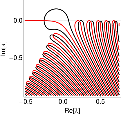
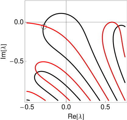
Figure 1: (Color online) Contour plot of zeros of the real (black) and the imaginary (red) parts of (6). Resolvent resonances appear where the contours intersect. The row of solutions close to the real axis correspond to the zeros of ${\rm Ai}$. Poles along $e^{-2i\pi/3}$ are close to zeros of ${\rm Ci}^{+}$. The resonance that originates in the bound state is marked by the circle in the right panel. On the left, the field is weak, and the resonance location is barely distinguishable from the ground-state energy $E_{\rm g}=-1/4$. Left: $F=0.025$, right: $F=0.125$. $A=1$.

Having obtained explicit expressions needed for the full resolvent (4) we now turn our attention to its poles. The denominator of the second part gives the equation to find the resonances, namely $1=AG_{0}(0,0,\lambda)$ which explicitly reads

$$1=\frac{\pi A}{F^{1/3}}{\rm Ai}\bigg{(}\frac{-\lambda}{F^{2/3}}\bigg{)}\left[i{\rm Ai}\bigg{(}\frac{-\lambda}{F^{2/3}}\bigg{)}+{\rm Bi}\bigg{(}\frac{-\lambda}{F^{2/3}}\bigg{)}\right]$$ (6)

This equation has infinitely many solutions; for a small $F$, zeros of ${\rm Ai}$ and ${\rm Ci}^{+}\equiv{\rm Bi}+i{\rm Ai}$ give rise to two families of resonances. However, we are interested in another solution which converges, with $F\!\to\!0$, to the zero-field ground-state energy $E_{\rm g}=-A^{2}/4$ on the real axis while approaching from the lower half-plane. Figure 1 illustrates all three types of solutions in weak and strong fields. The resonance corresponding to the metastable ground state is marked by a circle.

The real and imaginary parts of this resonance pole location $\lambda_{\rm R}=E_{\rm r}-iE_{\rm i}$ are related to the ionization rate and nonlinear polarizibility, respectively. Specifically, the ionization rate is proportional to its imaginary part

$$w=\frac{1}{\tau}=\frac{2E_{i}}{\hbar}\ .$$

A useful scaled quantity is the ionization rate in units of time given by the oscillation period of the driving field. If we specify the wavelength equivalently as the number $n$ of photon energies needed to overcome the system’s ionization potential $|E_{\rm g}|$, then the corresponding scaled ionization rate reads

$$w_{n}=2n\frac{E_{i}}{|E_{\rm g}|}$$

This quantity tells us if we should expect an appreciable fraction of atoms to be ionized within a single cycle of the optical field. For argon with its ionization potential of 15.7 eV and for the wavelength of 800 nm, $n=11$. We will therefore use $w_{11}$ to place our results in the context of femtosecond filamentation.

To relate $E_{\rm r}$ to the nonlinear polarization, we express the ground-state energy shift $E_{\rm r}-E_{\rm g}$ as the energy of an induced dipole in the electric field. In turn, the induced dipole is expressed through the field-dependent polarizibility $\alpha(E)$:

$$E_{r}-E_{g}=pE=\alpha(E)E^{2}$$

The nonlinear component of the polarizibility, namely $\alpha_{\rm NL}(E)=\alpha(E)-\alpha(0)$ is the quantity we aim to compare to the results of the higher-order Kerr measurement. As with the ionization rate, it is convenient to utilize a scaled form of the nonlinear polarizibility, namely

$$\chi_{\rm NL}=\alpha_{\rm NL}(E)/\alpha(0)$$

This quantity, termed scaled nonlinear susceptibility, measures the induced susceptibility of refraction relative to the linear-regime susceptibility of the unperturbed system.

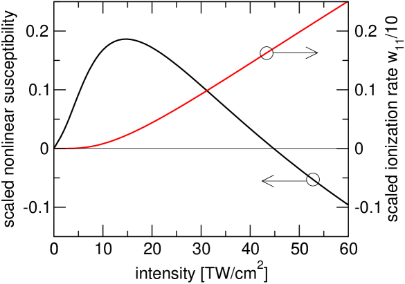
Figure 2: (Color online) Nonlinear susceptibility (black) and ionization rate (red) obtained from the exact solution for the resolvent pole.

We next discuss the properties of the exact solution to the resonance equation (6). We assume that the system has an ionization potential of 15.7 eV, i.e. that of argon, the incident pulse wavelength is 800 nm, and we express the field strength $F$ equivalently through the light intensity $I$. Figure 2 depicts the result obtained from the exact solution. The nonlinear susceptibility exhibits nearly linear increase for low intensity, which corresponds to the usual Kerr nonlinearity when the induced index of refraction is proportional to the light intensity. At higher intensities, $\chi_{\rm NL}(I)$ saturates and subsequently decreases into negative values. The zero crossing occurs at $I\approx 45$TW/cm². For very high intensities (not shown) the scaled susceptibility approaches $-1$ which corresponds to complete cancellation of the atom’s linear susceptibility. However, the extreme high-intensity regime is practically irrelevant because the survival probability of the ground state vanishes rapidly. The second curve in Fig. 2 shows the scaled ionization rate for the 800 nm driving wavelength. We can infer that in the vicinity of the susceptibility zero crossing, already a ten-cycle pulse is sufficient to reach ionization probability of about eighty percent. We can also see that when the nonlinear susceptibility starts to saturate, ionization already sets in. In other words, the nontrivial behavior of the nonlinear susceptibility is “synchronized” with significant ionization.

For a complementary view of the interplay between ionization and polarizibility, it is instructive to examine asymptotic solutions of (6) for weak fields. Previous works cavalcanti_decay_2003 ; Geltman1978 showed that the ionization rate is non-perturbative, and has the functional form of the tunneling ionization. This means that there exist no Taylor expansion in terms of the field strength. Because the polarizibility and ionization are connected through the resolvent pole location, it is only natural to expect that also the nonlinear index will be non-perturbative and lack proper Taylor expansion; this is indeed the case as illustrated next. In the lowest order (for $A=1$) the pole equation and its resonance solution $\lambda_{\rm R}$ become cavalcanti_decay_2003

$$1=\frac{i}{2\sqrt{\lambda}}-\frac{e^{-\frac{4(-\lambda)^{\frac{3}{2}}}{3F}}}{4\sqrt{\lambda}}\ \ \ ,\ \ \ \lambda_{\rm R}=-\frac{1}{4}-ie^{-\frac{1}{6F}}$$

The imaginary part gives rise to the non-perturbative tunneling ionization rate elberfeld_tunneling_1988 . Here one can see that there are actually two small parameters, namely $F$ and $e^{-\frac{1}{6F}}$. We develop the asymptotic solution of (6) in powers of these. For fixed expansion orders, we obtain a converged approximation in a finite number of iterations. The procedure shows that the real part of $\lambda_{\rm R}$ will also contain non-perturbative terms, starting with $e^{-\frac{1}{3F}}$. This means that neither ionization nor the polarizibility can be developed as a Taylor expansion in the field. A second important point is that even very high-order asymptotic solution can only reproduce the polarizibility curve roughly up to 10TW/cm² in Fig. 2. This is because the “small” parameter $e^{-\frac{1}{6F}}$ becomes large very quickly with increasing field. This sheds light on the fact that the measured nonlinear coefficients seem to represent a “divergent” function. The representation in powers of intensity, $\sum n_{2k}I^{k}$, is actually ill suited to represent this nonlinear behavior, and in our opinion contributes to the rather large error bars.

Finally, let us summarize our finding from the exact solution of the model system, and relate them to the questions posed in the introduction.

A) Most importantly, we can see that even a model with a single bound state exhibits an intensity dependent nonlinearity very much similar to that observed by Loriot et al., and that it occurs in the comparable intensity range. The absence of other bound states in the model indicates that the effect is due to virtual transitions into continuum. We speculate that, similarly to the high-harmonic generation, the few necessary “ingredients” are limited to the existence of ground state and of a continuum spectrum with the band-gap setting the scale for the intensity.

B) We showed that the nontrivial behavior in the polarizibility is intimately connected with the ionization, which sets in as soon as the susceptibility starts to saturate. Moreover, in this respect it is important to realize that in a real system the excited bound states will give rise to the additional $n_{2}I$ Kerr nonlinearity. This will then shift the real part of the total susceptibility toward higher intensities, while leaving the imaginary part intact. Consequently, the plasma generation will start before the nonlinearity changes its sign to de-focusing. From here we conjecture that in naturally occurring filaments, the higher-order nonlinearity will be effectively masked by free electrons. We speculate that this may very well be the answer to our question D), namely why previous experiments did not noticed these effects.

C) The fact that it is the continuum states that give rise to the nontrivial nonlinear behavior strongly suggests that the high-order nonlinearity will exhibit finite memory whose influence is likely to become stronger with increasing intensity. This is because unlike discrete states, the continuum of states can form “sufficiently many” superpositions which can “encode and remember” the history of the system. Of course, to verify this conjecture, time-resolved investigations will be necessary. If corroborated, a departure from a truly instantaneous (or very fast) nonlinearity will have an important consequence in decreasing the conversion efficiency in generation of high frequencies and supercontinuum.

To conclude, while keeping in mind the simplicity of the studied model, we believe that it gives us very important clues that will be eventually useful for understanding microscopic mechanisms controlling filamentation processes on few-femtosecond time scales.

Acknowledgment: This work was supported by the FCVV initiative of the Constantine the Philosopher University under grant no. I-06-399-01, and by the Air Force Office of Scientific Research under contract FA9550-10-1-0064.

References

- (1) A. Braun, G. Korn, X. Liu, D. Du, J. Squier, and G. Mourou, Opt. Lett. 20, 73 (1995).
- (2) V. Loriot, E. Hertz, O. Faucher, and B. Lavorel, Opt. Express 17, 13429 (2009).
- (3) V. Loriot, E. Hertz, O. Faucher, and B. Lavorel, Opt. Express 18, 3011 (2010).
- (4) P. Bejot, J. Kasparian, S. Henin, V. Loriot, T. Vieillard, E. Hertz, O. Faucher, B. Lavorel, and J.-P. Wolf, Phys. Rev. Lett. 104, 103903 (2010).
- (5) M. Nurhuda, A. Suda and K. Midorikawa, New Journal of Physics 10, 053006 (2008).
- (6) R. W. Boyd, Nonlinear Optics (Academic Press, 2008).
- (7) H. L. Cycon, R. Froese, W. Kirsch, and B. Simon, Schrödinger Operators (Springer-Verlag, 1987).
- (8) S. Albeverio and P. Kurasov, Singular perturbations of diferential operators (Cambridge University Press, 2000).
- (9) V. M. Villalba and L. A. González-Díaz, The European Physical Journal C 61, 519 (2009).
- (10) L. Peng and A. F. Starace, J. Chem. Phys. 125, 154311 (2006).
- (11) H. Uncu, H. Erkol, E. Demiralp, and H. Beker, Central European Journal of Physics 3, 303 (2005).
- (12) G. V. Dunne and C. S. Gauthier, Phys. Rev. A 69, 053409 (2004).
- (13) G. Alvarez and B. Sundaram, J. Phys. A: Math. and Gen. 37, 9735 (2004).
- (14) W. Elberfeld and M. Kleber, Z. Phys. B: Cond. Matt. 73, 23 (1988).
- (15) S. Geltman, J. Phys. B: Atom. Molec. Phys. 11, 3323 (1978).
- (16) R. M. Cavalcanti, P. Giacconi, and R. Soldati, J. Phys. A: Math. and Gen. 36, 12065 (2003).
- (17) G. P. Arrighini and M. Gavarini, Lettere Al Nuovo Cimento Series 2 33, 353 (1982).
- (18) M. Abramowitz and I. A. Stegun, Handbook of Mathematical Functions with Formulas, Graphs, and Mathematical Tables (New York: Dover Publications, 1972).