Self-Similar Solutions of Triaxial Dark Matter Halos

Abstract

We investigate the collapse and internal structure of dark matter halos. We consider halo formation from initially scale-free perturbations, for which gravitational collapse is self-similar. Fillmore and Goldreich (1984) and Bertschinger (1985) solved the one dimensional (i.e. spherically symmetric) case. We generalize their results by formulating the three dimensional self-similar equations. We solve the equations numerically and analyze the similarity solutions in detail, focusing on the internal density profiles of the collapsed halos. By decomposing the total density into subprofiles of particles that collapse coevally, we identify two effects as the main determinants of the internal density structure of halos: adiabatic contraction and the shape of a subprofile shortly after collapse; the latter largely reflects the triaxiality of the subprofile. We develop a simple model that describes the results of our 3D simulations. In a companion paper, we apply this model to more realistic cosmological fluctuations, and thereby explain the origin of the nearly universal (NFW-like) density profiles found in N-body simulations.

1. Introduction

As the Universe expands, small fluctuations in the dark matter density grow in amplitude. Eventually, these dark matter fluctuations grow nonlinear, leading to collapse and virialization into structures termed halos. The internal structure of dark matter halos has long been a topic of interest. Halo structure significantly affects galaxy formation and evolution, since galaxies form at the centers of halos. It can also have implications for dark matter detection, which depends strongly on the dark matter density inside collapsed objects.

N-body simulations have shown that halos forming in hierarchical, Cold Dark Matter (CDM) cosmologies have fairly generic density profiles. Navarro, Frenk, & White (“NFW,” 1996, 1997) suggested that CDM halos have universal profiles, with $\rho\propto r^{-3}$ at large radii and $\rho\propto r^{-1}$ at small radii. Subsequent numerical work found qualitatively similar results (e.g. Moore et al., 1998; Diemand et al., 2007; Gao et al., 2008; Stadel et al., 2009; Diemand et al., 2008; Navarro et al., 2010), although the precise shape of the innermost profile is still under debate.

It has proven a long-standing puzzle to explain why halos are well described by the NFW profile. Identifying the important processes using conventional cosmological N-body simulations has been challenging, in part because of the limited dynamic range of such simulations. If the mechanism setting halo profiles is truly generic, however, then we can investigate it using particular test cases that can be studied in great detail. One standard technique for achieving high resolution is to study problems that admit self-similar solutions, which is the approach we follow in this paper.

Fillmore & Goldreich (1984) and Bertschinger (1985) calculated the self-similar collapse of spherically symmetric profiles. They considered the evolution of a linear overdensity of the form $\delta_{\rm lin}\propto r^{-\gamma}$ in a flat CDM Universe. This problem has only a single characteristic lengthscale, $r_{*}$, which is where the overdensity is of order unity. Inside of $r_{*}$ a virialized halo forms, and outside of $r_{*}$ density perturbations remain small and linear. As time proceeds, the virialized halo grows by accreting from its surroundings, and $r_{*}$ increases. Yet the properties of the halo and its surroundings are independent of time when scaled relative to $r_{*}$. The interior density of the virialized halo scales as a power-law in radius, $\rho\propto r^{-g}$, where $g=2$ for $\gamma\leq 2$, and $g=3\gamma/(1+\gamma)$ for $\gamma\geq 2$ (Fillmore & Goldreich, 1984). Hence the interior slope is always much steeper than the interior NFW slope.

Subsequent work expanded upon this analysis. Ryden (1993) calculated the self-similar collapse of axisymmetric profiles. She showed that $\gamma=2$ yielded an inner slope of $-g\simeq-2$, in accord with the spherically symmetric prediction. But $\gamma=1$ yielded $-g\approx-1.5$. Surprisingly, the work of Ryden (1993) has not been followed up in the literature. In particular, it has not yet been extended to three dimensions, which is the focus of the present paper.

As we describe below, a number of authors have used qualitative arguments, as well as model equations, to argue that self-similar, triaxial collapse should produce asymptotic inner slopes given by the Fillmore-Goldreich expression $g=3\gamma/(1+\gamma)$ for all $\gamma$. (e.g. White & Zaritsky, 1992; Nusser, 2001; Ascasibar et al., 2004, 2007). In this paper, we shall confirm with our solutions of the exact equations that this indeed holds true, although in some cases this slope is only reached on scales $\lesssim 10^{-5}$ of the virial radius.

More recently, Vogelsberger et al. (2010) carried out N-body simulations initialized with the spherically symmetric initial conditions of Fillmore & Goldreich (1984). They found that even though the initial conditions are spherically symmetric, the radial orbit instability acts to make the evolution non-spherical. Zukin & Bertschinger (2010) considered spherical self-similar solutions, but with a prescription based on tidal torques for generating non-radial velocities.

In this paper, we consider the evolution of a linear overdensity of the form $\delta_{\rm lin}=f(\theta,\phi)r^{-\gamma}$, where $f$ is an arbitrary function of zenith and azimuth. We emphasize that we solve the exact evolutionary equations, and our solutions are exact, subject only to numerical errors. In this sense, our nonspherical solutions differ from previous models of nonspherical collapse (e.g., Eisenstein & Loeb, 1995; Bond & Myers, 1996) that resorted to model equations.

The paper is structured as follows. In §2, we describe our method for obtaining the self-similar solutions to the equations of motion governing the collapse of initially scale-free perturbations. In §3, we introduce an oversimplified model—the “frozen model”—that will prove helpful in interpreting the results of the full simulations. In §4, we review the spherically symmetric solutions of Fillmore & Goldreich (1984); Bertschinger (1985). In §5, we present the solution to axisymmetric collapse. In §6, the heart of this paper, we present a suite of 3D self-similar solutions, and analyze them in detail, with the primary goal of isolating the physics that is responsible for the interior density profiles. In §7, we introduce a toy model that incorporates the mechanisms that we identified in §6. In Dalal et al. (2010) we apply the toy model to more realistic cosmological fluctuations, and show that NFW-like profiles are a generic outcome of the dissipationless collapse of peaks of Gaussian random fields.

2. Self-Similar Equations and Method of Solution

2.1. Equations of Motion

We consider a region of space in a flat CDM Universe that has linear overdensity

$$\delta_{\rm lin}(\mbox{\boldmath$r$\unboldmath})={\rm const}\times r^{-\gamma}f(\theta,\phi)$$ (1)

at a fixed time, where $r$ is the proper radial displacement from the origin, $\gamma$ is a constant and $f$ is an arbitrary function of zenith and azimuth. As long as the overdensity satisfies $|\delta|\ll 1$, linear perturbation theory implies that

$$\delta(t,\mbox{\boldmath$r$\unboldmath}) = t^{2/3}\left({r\over t^{2/3}}\right)^{-\gamma}f(\theta,\phi)$$ (2)

$$= \left({r\over r_{*}(t)}\right)^{-\gamma}f(\theta,\phi)\ ,\ \ \ ({\rm for}\ \delta\ll 1)$$ (3)

where

$$r_{*}(t)\equiv t^{{2\over 3}+{2\over 3\gamma}}\ ,$$ (4)

and we have absorbed a constant prefactor into $f$. The quantity $r_{*}(t)$ is, aside from a multiplicative constant, equal to the characteristic lengthscale at which nonlinearities become important ($\delta\sim 1$). As we now show, the evolution is self-similar when all lengthscales are scaled to $r_{*}$.

A particle’s equations of motion are

$${d{\mbox{\boldmath$r$\unboldmath}}\over dt} = v$$ (5)

$${d{\mbox{\boldmath$v$\unboldmath}}\over dt} = -\mbox{\boldmath$\nabla_{r}$\unboldmath}\phi\ ,$$ (6)

where $r$ and $v$ are its position and velocity, and $\phi$ is the gravitational potential (not to be confused with the azimuthal angle). Different particles may be labelled by their positions $\mbox{\boldmath$r$\unboldmath}_{i}$ at an initial time $t_{i}$,

$$\mbox{\boldmath$r$\unboldmath}=\mbox{\boldmath$r$\unboldmath}(t,{\mbox{\boldmath$r$\unboldmath}_{i}})\ ,\ \mbox{\boldmath$v$\unboldmath}=\mbox{\boldmath$v$\unboldmath}(t,{\mbox{\boldmath$r$\unboldmath}_{i}})\ ,$$ (7)

where $t_{i}$ is chosen to be sufficiently small that all particles of interest expand with the Hubble flow at that time.

Scaling lengths with $r_{*}$ and times with $t$, we define the scaled radius and velocity $(\mbox{\boldmath$R$\unboldmath},\mbox{\boldmath$V$\unboldmath})$ via

$$\mbox{\boldmath$r$\unboldmath}(t,\mbox{\boldmath$r$\unboldmath}_{i}) = r_{*}\mbox{\boldmath$R$\unboldmath}(s,\theta_{i},\phi_{i})$$ (8)

$$\mbox{\boldmath$v$\unboldmath}(t,\mbox{\boldmath$r$\unboldmath}_{i}) = {r_{*}\over t}\mbox{\boldmath$V$\unboldmath}(s,\theta_{i},\phi_{i})\ ,$$ (9)

where

$$s\equiv{r_{i}\over r_{*}}\left({t\over t_{i}}\right)^{2/3}\$$ (10)

is the scaled initial comoving radius. We shall employ $s$ as our independent radial variable; it is a Lagrangian co-ordinate that labels particles by their initial radius. Its form may be understood as follows. At early times a particle expands with the Hubble flow, and hence its $r_{i}$ depends on $t_{i}$ via $r_{i}\propto t_{i}^{2/3}$. Therefore different particles may be labelled by their value of $r_{i}/t_{i}^{2/3}$. Scaling $r_{i}$ with $r_{*}$ and $t_{i}$ with $t$ leads to our form for $s$. Equivalently, each particle may be labelled by the mass it initially enclosed as it expanded with the Hubble flow, $m_{i}=(4\pi/3)\bar{\rho}(t_{i})r_{i}^{3}$, where $\bar{\rho}=1/(6\pi t^{2})$ is the background density of a homogeneous flat Universe. Therefore its scaled initial mass

$$M_{i}\equiv{m_{i}\over r_{*}^{3}/t^{2}}={2\over 9}s^{3}$$ (11)

is a simple function of $s$.

Since the gravitational potential has units of velocity squared, we define the scaled potential $\Phi$ via

$$\phi(t,{\mbox{\boldmath$r$\unboldmath}})\equiv{r_{*}^{2}\over t^{2}}\Phi(\mbox{\boldmath$R$\unboldmath})\ .$$ (12)

The equations of motion then become

$${d\over d\ln s}\left(\begin{array}[]{c}{\mbox{\boldmath$R$\unboldmath}}\\ {\mbox{\boldmath$V$\unboldmath}}\end{array}\right)=\left(\begin{array}[]{cc}\gamma+1&-{3\gamma\over 2}\\ 0&1-{\gamma\over 2}\end{array}\right)\left(\begin{array}[]{c}{\mbox{\boldmath$R$\unboldmath}}\\ {\mbox{\boldmath$V$\unboldmath}}\end{array}\right)+{3\gamma\over 2}\left(\begin{array}[]{c}0\\ {\mbox{\boldmath$\nabla$\unboldmath}_{R}\Phi}\end{array}\right)$$ (13)

It remains to calculate $\Phi({\mbox{\boldmath$R$\unboldmath}})$. Given the trajectories $\mbox{\boldmath$r$\unboldmath}(t,\mbox{\boldmath$r$\unboldmath}_{i})$ for all particles, one can calculate the corresponding mass density, and then invert Poisson’s equation to yield the potential. Consider the particles that at time $t_{i}$ lie near ${\mbox{\boldmath$r$\unboldmath}}_{i}$, within the volume element $d^{3}{\mbox{\boldmath$r$\unboldmath}_{i}}$. The mass in these particles is

$$dm = \rho(t_{i},{\mbox{\boldmath$r$\unboldmath}}_{i})d^{3}{\mbox{\boldmath$r$\unboldmath}_{i}}$$ (14)

$$= {1\over 6\pi t_{i}^{2}}d^{3}{\mbox{\boldmath$r$\unboldmath}_{i}}$$ (15)

where $\rho$ is the mass density, which at time $t_{i}$ is given by the background density. By mass conservation, the density $\rho$ at position $\mbox{\boldmath$r$\unboldmath}=\mbox{\boldmath$r$\unboldmath}(t,\mbox{\boldmath$r$\unboldmath}_{i})$ due to these particles is given by

$$\rho(t,\mbox{\boldmath$r$\unboldmath}|\mbox{\boldmath$r$\unboldmath}_{i})d^{3}\mbox{\boldmath$r$\unboldmath}={1\over 6\pi t_{i}^{2}}d^{3}{\mbox{\boldmath$r$\unboldmath}_{i}}\ .$$ (16)

The third argument of $\rho$ (i.e. $\mbox{\boldmath$r$\unboldmath}_{i}$) is necessary because particles with different vaues of $\mbox{\boldmath$r$\unboldmath}_{i}$ can contribute to the density at position $r$ due to shell crossing. The total density is the sum of the above $\rho$ over all $\mbox{\boldmath$r$\unboldmath}_{i}$ such that $\mbox{\boldmath$r$\unboldmath}=\mbox{\boldmath$r$\unboldmath}(t,\mbox{\boldmath$r$\unboldmath}_{i})$.

We denote the scaled density with a capital $\rho$ (=$P$), defined via

$$\rho(t,\mbox{\boldmath$r$\unboldmath}|\mbox{\boldmath$r$\unboldmath}_{i})={1\over t^{2}}P(\mbox{\boldmath$R$\unboldmath}|\mbox{\boldmath$s$\unboldmath})\ ,$$ (17)

in which case the scaled version of equation (16) is

$$P(\mbox{\boldmath$R$\unboldmath}|\mbox{\boldmath$s$\unboldmath})d^{3}\mbox{\boldmath$R$\unboldmath}={d^{3}{\mbox{\boldmath$s$\unboldmath}}\over 6\pi}\ ,$$ (18)

where we have introduced the vector

$${\mbox{\boldmath$s$\unboldmath}}\equiv{{\mbox{\boldmath$r$\unboldmath}_{i}}\over r_{*}}\left({t\over t_{i}}\right)^{2/3}\ .$$ (19)

The total density is the sum over all streams that contribute to $R$:

$$P({\mbox{\boldmath$R$\unboldmath}})=\sum_{\mbox{\boldmath$s$\unboldmath}:\mbox{\boldmath$R$\unboldmath}(\mbox{\boldmath$s$\unboldmath})=\mbox{\boldmath$R$\unboldmath}}P(\mbox{\boldmath$R$\unboldmath}|\mbox{\boldmath$s$\unboldmath})\ .$$ (20)

Henceforth the symbol $P$ without an argument will denote the total density $P(\mbox{\boldmath$R$\unboldmath})$.

Given $P$, one can solve for $\Phi$ by inverting the scaled Poisson equation

$$\nabla_{R}^{2}\Phi=4\pi P\ .$$ (21)

Equations (13), (18), and (21) are the self-similar equations. They form a closed system. Note that $t$, $r_{*}$, $t_{i}$, and $r_{i}$ only enter these equations in the combination $s$. The self-similar equations are exact, following directly from the definitions of $r_{*}$ and the scaled variables. Therefore the evolution is self-similar when the linear density field can be written as a function of the scaled variables, i.e. when it has the form given by equation (1).

2.2. Method of Solution

We solve the self-similar equations iteratively. The scaled density is first set to its linear value everywhere, i.e., to

$$P({\mbox{\boldmath$R$\unboldmath}})=P_{\rm lin}({\mbox{\boldmath$R$\unboldmath}})\equiv{1\over 6\pi}\left(1+R^{-\gamma}f(\theta,\phi)\right)\ ,$$ (22)

where $f$ is any prescribed function and $0<\gamma<3$. Inverting Poisson’s equation determines $\Phi({\mbox{\boldmath$R$\unboldmath}})$. We use this $\Phi$ to integrate the trajectories of particles. Each particle is initialized at large $s$, where it expands with the Hubble flow: ${\mbox{\boldmath$R$\unboldmath}_{0}}={\mbox{\boldmath$s$\unboldmath}},{\mbox{\boldmath$V$\unboldmath}_{0}}={2\over 3}{\mbox{\boldmath$s$\unboldmath}}$. Its subsequent trajectory is determined by integrating equation (13) from large to small $s$ with fixed $\Phi(\mbox{\boldmath$R$\unboldmath})$. At each step $ds$ of this integration, we record how much the particle contributes to the local density (eq. [18]). Repeating this integration for particles at all initial $\theta$ and $\phi$ produces the full density field $P({\mbox{\boldmath$R$\unboldmath}})$. Inverting Poisson’s equation then determines the new $\Phi({\mbox{\boldmath$R$\unboldmath}})$, which is used in the second iteration step. This cycle continues until successive $\Phi$’s agree with each other, which typically takes 10-20 iteration steps, depending on the simulation parameters. See §A for a more detailed description of our method.

3. Frozen Model

At large radii, $r\gtrsim r_{*}(t)\equiv t^{{2\over 3}+{2\over 3\gamma}}$, the evolution is linear and particles nearly expand with the Hubble flow. Eventually $r_{*}(t)$ will overtake such particles, whereupon their evolution becomes nonlinear and they gravitationally collapse. In the present section, we ask what the density profile would be if, instead of collapsing, each particle’s proper radius remained frozen as soon as it crossed $r_{*}$. This is essentially identical to the “circular orbit” model of Ryden & Gunn (1987), in which mass shells are placed on circular orbits with energy equalling that at turnaround. Their circular-orbit model freezes shells at half the turnaround radius, while our frozen model freezes shells at $r_{*}$, and so the resulting profiles are identical up to an overall rescaling. The key feature is that both of these models avoid shell crossing. Although this frozen model is unphysical, it is useful as a baseline to compare against the full evolution.

Figure 1.— Frozen Model Mass Profile ($\gamma=2.5$): The solid line shows the enclosed mass profile $m(t,r)$ at time $t_{0}=0.01$, and the dashed line shows it at time $t_{1}=1$. At large radii, $r>r_{*}(t)$, particles expand with the Hubble flow, and the enclosed mass is given by the background expression $(2/9)r^{3}/t^{2}$. At small radii, particles are frozen. Hence the form of $r_{*}(t)$ dictates the profile at $r<r_{*}$.

Figure 1 shows two snapshots of the enclosed mass profile,

$$m(t,r)\equiv 4\pi\int_{0}^{r}{\rho}(t,r)r^{2}dr\ ,$$ (23)

in this model. At radii larger than $r_{*}$, the enclosed mass profile is the product of the background density $=1/(6\pi t^{2})$ and the volume of a sphere of radius $r$, i.e., $m=(2/9)r^{3}/t^{2}$. At radii smaller than $r_{*}$, the mass profile is time-independent because of the frozen assumption, and thus $m=(2/9){r^{3}/t_{*}(r)^{2}}$, where $t_{*}(r)$ is the inverse of $r_{*}(t)$; i.e., the frozen mass profile is

$$m=\cases{{2\over 9}r^{3/(1+\gamma)},&if $r<r_{*}$\cr{2\over 9}{r^{3}\over t^{2}},&if $r>r_{*}$\cr}$$ (24)

It follows that the interior density profile scales as

$$\rho\propto r^{-g_{f}}\ ,$$ (25)

where

$$g_{f}\equiv{3\gamma\over\gamma+1}\ ;$$ (26)

we call $-g_{f}$ the frozen slope.

Real collapsing solutions—in 1D as well as in 3D—are obviously more complicated than the frozen model. We distinguish two effects, either of which may cause the interior spherically-averaged density profile to deviate from the frozen slope:

1. Shell Profiles: Consider the set of particles that initially lie in a thin spherical shell that expands with the Hubble flow. In the frozen model, it is assumed that once the radial co-ordinates of these shell particles cross $r_{*}$, they freeze; hence they lay down a density profile that vanishes everywhere except at the distance at which they freeze. By contrast, in the actual self-similar solutions, shell particles lay down an extended density profile as they execute their orbits, which we call the “shell profile.” The shape of the tail of the shell profile (i.e. for $r\rightarrow 0$) can affect the total density profile at small radii.

2. Shrinking Apoapses: The apoapses of shell particles can gradually shrink in time, rather than the particles remaining frozen.

As we shall show, in general both shell profiles and shrinking apoapses are present in the full solutions. But even when they do occur, they do not necessarily cause the interior density profile to deviate from the frozen slope at very small radii. In particular, the total density slope will be $-g_{f}$ as long as

1. each shell tail remains shallower than $-g_{f}$; and,

2. the apoapses eventually stop shrinking after a finite time

3.1. Lagrangian Variables $r_{f}$ and $t_{f}$

When considering the evolution of particles in the self-similar solutions, it will prove convenient to employ new Lagrangian variables based on the frozen model. In place of $t_{i}$ and $r_{i}$ (eq. [7]), we define $r_{f}$ as the radius at which a particle with given initial $r_{i}$ and $t_{i}$ would freeze in the frozen model; similarly, we define $t_{f}$ as its time of freeze-out in the frozen model. Since $r_{f}=r_{*}(t_{f})$ and $r_{f}/r_{i}=(t_{f}/t_{i})^{2/3}$, we have

$${r_{f}} \equiv \left(r_{i}^{3}/t_{i}^{2}\right)^{(1+\gamma)/3}$$ (27)

$$t_{f} \equiv \left(r_{i}^{3}/t_{i}^{2}\right)^{\gamma/2}\ .$$ (28)

Scaling relative to $r_{*}$ and $t$ yields

$${r_{f}\over r_{*}}=s^{1+\gamma}\ ,\ \ \ {t_{f}\over t}=s^{3\gamma/2}\ .$$ (29)

4. Spherically Symmetric Solutions

We review here the well-known spherically symmetric self-similar solutions (Fillmore & Goldreich, 1984; Bertschinger, 1985), focussing in particular on the interior density profile. The linear density field is prescribed to be $\propto R^{-\gamma}$, independent of $\theta$ and $\phi$. Note that our parameter $\gamma$ is related to Fillmore & Goldreich’s $\epsilon$ via $\gamma=3\epsilon$ for their spherically symmetric solutions. In these solutions, all particles have purely radial trajectories, and hence are forced to cross through the origin repeatedly after collapse. We describe the spherical solution in great detail, in order to lay the groundwork for our discussion of the more complicated triaxial similarity solutions.

In spherically symmetric collapse, the density profile for $R\ll 1$ scales as

$$P\propto R^{-g}\ ,$$ (30)

where

$$g=\cases{g_{f}\equiv 3\gamma/(1+\gamma),&for $\gamma>2$\cr 2,&for $\gamma<2$\cr}$$ (31)

(Fillmore & Goldreich, 1984; Bertschinger, 1985), i.e., the slope differs from the frozen slope when $\gamma<2$. To illustrate the reason for this behavior, and to set the stage for the more complicated non-spherical cases, we present two spherical simulations, with $f=1$ in equation (22): one simulation with $\gamma>2$ and the other with $\gamma<2$.

4.1. Spherical simulation with $\gamma=2.5$

Figure 2.— Density Profiles (spherical symmetry, $\gamma=2.5$): The black curve shows the self-similar density profile $P$, normalized by the background density $1/6\pi$. At small $R$, it asymptotes to the frozen slope $-g_{f}=-15/7$. The colored curves show “shell profiles,” i.e. the density contributed by particles that initially lay within the same thin shell. For example, the curve labelled $-2$ shows the density of particles that have $10^{-3}<M_{i}<10^{-2}$, and subsequent curves show subsequent decades in $M_{i}$.

Figure 3.— Enclosed Mass Profiles (spherical symmetry, $\gamma=2.5$): Each colored curve shows the mass profile from all shells interior to a given initial shell. For example, the blue curve labelled 0 shows the enclosed mass profile from all shells with $M_{i}<10^{0}$. The upper envelope of the colored curves shows the enclosed mass profile. The dashed line is the mass profile in the frozen model. The stars on each shell profile indicate the location of the shell’s current apoapse.

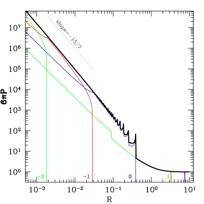
Figures 2-4 show results from the spherical solution with $\gamma=2.5$. Figure 2 shows the total density profile ($P$) as a black line, normalized to the background density ($=1/6\pi)$. At small $R$, the slope is given by the frozen slope $-g_{f}=-15/7=-2.14$. The colored lines show “shell profiles,” i.e. the density contributed by particles that initially lay within the same thin shell, also normalized by $6\pi$. For example, the blue curve labelled 0 shows the density from all particles that have scaled initial mass $10^{-1}<M_{i}<10^{0}$. The red curve, which lies deeper in, comes from a shell with smaller initial mass, $10^{-2}<M_{i}<10^{-1}$, etc. The total density is the sum of the shell profiles. It is apparent that the density at small $R$ is dominated by shells with small $M_{i}$, and the smaller the $R$ the smaller the $M_{i}$ that contribute.

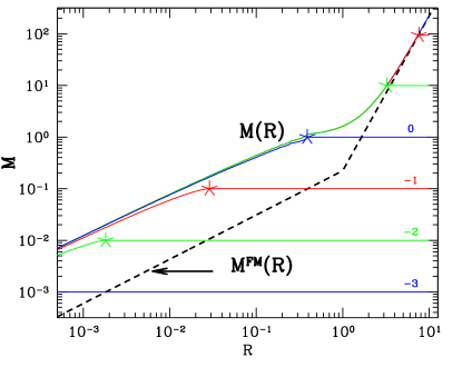
Figure 3 shows the enclosed mass profiles

$$M(R)\equiv 4\pi\int_{0}^{R}P(R^{\prime})R^{\prime 2}dR^{\prime}\ .$$ (32)

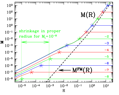
The upper envelope of the colored curves is the $M(R)$ that results from the total density profile shown in Figure 2. The individual colored curves show the enclosed mass profiles from all shells interior to a given shell. For example, the blue curve labelled 0 shows the enclosed mass profile from all shells with $M_{i}<10^{0}$, the red curve labelled -1 shows the profile from all shells with $M_{i}<10^{-1}$, etc. Note that the blue curve asymptotes at large $R$ to $M=10^{0}$, the red to $M=10^{-1}$, etc.

Also shown in Figure 3 as a dashed line is the mass profile in the frozen model (see Fig. 1). The outer radius of each colored profile is marked with a star. From the fact that the stars are parallel to the frozen profile at small $R$ indicates that particles’ apoapses do not continue to shrink after collapsing.

Figure 4.— Particle Trajectory (spherical symmetry, $\gamma=2.5$): The solid curve shows a particle’s proper radius versus time, where the radius is scaled relative to the frozen radius and the time relative to the frozen time (eq. [29]). At late times, the apoapses are nearly constant. The stars are equivalent to the ones in Figure 4, converted with equation (11). The dashed curve shows the trajectory in the frozen model.

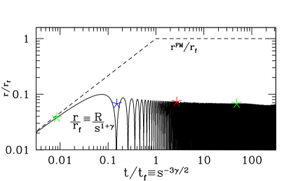
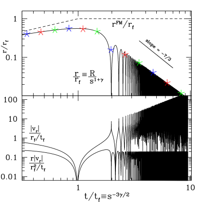
The apoapse evolution may also be seen directly in Figure 4, which shows the time evolution of the proper radius of a single particle (and hence of all particles). The self-similar solution yields the function $R(s)$, which we convert to the function $r(t)$ (scaled relative to the particle’s $r_{f}$ and $t_{f}$) with the aid of equations (29). The particle’s proper radius reaches turnaround at $t/t_{f}\sim 0.08$. Thereafter, its apoapse remains roughly constant (although it does shrink very slightly at late times). Also shown in Figure 4 are the stars from Figure 3, where the co-ordinates $(R,M\equiv M_{i})$ of each star in the latter figure are converted to Figure 4 with the aid of equations (11) and (29); the stars clearly trace the particle’s apoapse.

4.2. Spherical Simulation with $\gamma=0.25$

Figure 5.— Density Profiles (spherical symmetry, $\gamma=0.25$): The black curve shows the total density, and the colored curves the shell profiles; see caption of Fig. 2 for detail. The total density has logarithmic slope $-2$, much steeper than the frozen slope, because it is dominated by particles with $10^{-4}<M_{i}<10^{-3}$ (the blue curve labelled -3).

Figure 6.— Enclosed Mass Profiles (spherical symmetry, $\gamma=0.25$): See caption of Figure 3 for description.

Figure 7.— Particle Trajectory and Velocity (spherical symmetry, $\gamma=0.25$): The top panel shows a particle’s proper radius versus time. At late times, the apoapses shrink. The bottom panel shows the radial velocity and the product $r|v_{r}|$ relative to the frozen values. From the fact that the envelope of the $r|v_{r}|$ oscillations remains constant, we infer that the radial adiabatic invariant is very nearly constant.

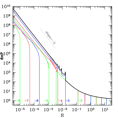
Figures 5-7 show results from a spherical simulation with $\gamma=0.25$. Throughout the rest of the paper, we will frequently use $\gamma=0.25$ calculations to illustrate important aspects of the self-similar solutions, in part because the effective profiles of peaks of Gaussian random fields in CDM cosmologies have comparably shallow interior slopes (see Dalal et al., 2010, for more detail). Figure 5 shows the total density profile, as well as individual shell profiles. At small $R$, the logarithmic slope of the total density is $-2$, which is much steeper than than the frozen slope $-3\gamma/(1+\gamma)=-0.6$. From the shell profiles it is clear why the total density profile is more concentrated than the frozen profile: the blue curve labelled -3, which represents particles with $10^{-4}<M_{i}<10^{-3}$, shows that these particles lay down a density profile with slope $-2$. These particles dominate the total density profile all the way to $R\rightarrow 0$. Hence the total density slope reflects theirs. This behavior is in sharp contrast to that seen in the $\gamma>2$ simulation (Fig. 2), where the density profile at increasingly small $R$ is dominated by particles with increasingly small $M_{i}$ (Fillmore & Goldreich, 1984).

The reason that the individual shell profile has slope $-2$ may be understood qualitatively as follows. (See Fillmore & Goldreich (1984) for the quantitative calculation.) If we consider only particles from the same initial shell, then the mass they contribute within a sphere of radius $R$ is proportional to $\delta t(R)$, the amount of time the particles spend inside of that radius in the course of an orbit. Here, we assume that $R$ is smaller than their apoapse, and that the mass profile is averaged over a timescale of order the orbital time; we also ignore the distinction between the scaled and unscaled $R$ because at late times the scaling factor changes negligibly over the course of a single orbit. Since the interior gravitational potential depends weakly on $R$, the speed of a particle remains fairly constant as it plunges from its apoapse, through $R=0$, to its next apoapse. Therefore $M(R)\propto\delta t(R)\propto R$, and the resulting density profile is proportional to $R^{-2}$.

Figure 6 shows the enclosed mass profile, as well as the enclosed mass profiles from cumulated shells. It is clear from this figure as well that particles with a narrow range of $M_{i}$ dominate the total profile all the way to $R\rightarrow 0$. This figure shows a second feature of spherical solutions with $\gamma<2$: the stars that denote the outermost radii of cumulated shells are not parallel to the profile of the frozen model (the dashed line in the figure). This shows that the apoapses of shells with increasingly small $M_{i}$ decrease relative to the frozen profile–i.e., that a given shell’s apoapses shrink in time.

The top panel of Figure 7 shows the shrinking of the apoapses directly. The bottom panel shows the radial velocity, scaled appropriately, as well as its product with the radius. After the particle has collapsed, its radial adiabatic invariant is proportional to $\oint v_{r}dr$, integrated over an orbit. From the fact that the envelope of oscillations of $r|v_{r}|$ remains constant, we infer that the adiabatic invariant is constant after collapse.

The constancy of the adiabatic invariant, together with the virial theorem, gives the rate at which the apoapse radius, $r_{a}$, shrinks at late times (Fillmore & Goldreich, 1984). The interior mass profile scales linearly with radius: $m(t,r)={\rm const}\times(r_{*}^{3}/t^{2})(r/r_{*})$, where the factors of $r_{*}$ and $t$ are as required to convert from scaled to unscaled variables. Therefore the virial theorem ($m(t,r_{a})={\rm constant}\times v^{2}r_{a}$, where $v$ is a typical speed—e.g. the r.m.s. speed) together with the constancy of the adiabatic invariant ($r_{a}v=$constant) imply that the amplitude of radial oscillations shrinks in inverse proportion to the enclosed mass,

$$r_{a}\propto 1/m(t,r_{a})\ ,$$ (33)

and hence

$$r_{a}\propto t^{-({2\over 3\gamma}-{1\over 3})}\ ,\ \ \gamma<2\ ,$$ (34)

(Fillmore & Goldreich, 1984). The top panel of Figure 7 confirms that $r_{a}\propto t^{-7/3}$ at late times.

5. Axisymmetric Solutions

For axisymmetric solutions, the linear density field is prescribed to be $\propto f(\theta)R^{-\gamma}$ (eq. [22]), i.e. $f$ is independent of $\phi$ . This implies that particles can never acquire a $\phi$-component to their velocities, and hence they must cross through the central axis of symmetry repeatedly after collapse.

In spherically symmetric solutions an individual shell’s density profile has logarithmic slope -2 after collapse. Therefore whenever $g_{f}<2$, the slope of an individual shell is steeper than that of the frozen slope, and hence recently collapsed shells dominate the interior density, driving the interior total density to a slope of -2.

But in axisymmetric solutions, an individual shell’s density profile has logarithmic slope -1. To see this, we consider the cylindrical co-ordinates of a particle $(R_{cyl},\theta_{cyl},Z_{cyl})$. Because of the axisymmetric assumption, the particle’s $\theta_{cyl}\equiv\phi$ remains constant over the course of its orbit, and only its $R_{cyl}$ and $Z_{cyl}$ change. As it traces out a trajectory in the $R_{cyl}-Z_{cyl}$ plane, its speeds in the $R_{cyl}$ and $Z_{cyl}$ directions are nearly constant (§4.2), and for a typical particle we may take these two speeds to be comparable to each other. If we assume that the particle’s orbit is chaotic, the amount of time it spends within a distance $R$ of the origin (where $R$ is less than its apoapse) is proportional to the area of that region in the $R_{cyl}-Z_{cyl}$ plane, i.e. $\delta t(R)\propto R^{2}$. Equivalently, the amount of time a particle spends inside a sphere of radius $R$ centered on the origin also scales as $\delta t(R)\propto R^{2}$. Since the mass enclosed within that sphere is proportional to $\delta t$, it follows that $M\propto R^{2}$, and hence that the density scales as $P\propto R^{-1}$.

Reasoning as before, we conclude that axisymmetric solutions should have interior density that scales as $P\propto R^{-g}$ , where

$$g=\cases{g_{f}\equiv 3\gamma/(1+\gamma),&for $\gamma>1/2$\cr 1,&for $\gamma<1/2$\cr}$$ (35)

Ryden (1993) calculated axisymmetric solutions for two values of $\gamma>1/2$—specifically, $\gamma=1$ and 2. The resulting interior density profiles have logarithmic slopes that are indeed close to $-g_{f}$, i.e. to -1.5 and -2, respectively, in agreement with equation (35).

Figure 8.— Axisymmetric Solution ($\gamma=0.25$, $e=0.1$, $p=0.1$): The black curve shows the total angle-averaged density profile. The colored curves show the shell profiles. The frozen slope for this value of $\gamma$ is $-g_{f}=-0.6$. Since the profile of an individual shell has logarithmic slope -1, steeper than the frozen slope, recently collapsed shells dominate the interior total density, and drive its slope to -1. The largest shell profile (red) is from particles with $M_{i}>10^{-3.4}$; the next shell profile (green) is from $10^{-4.4}<M_{i}<10^{-3.4}$, and subsequent profiles are from subsequent decades in $M_{i}$.

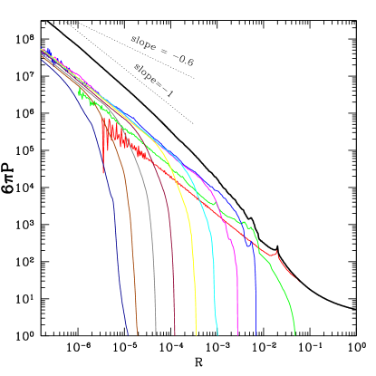
Figure 8 shows an axisymmetric simulation with $\gamma=0.25$ (and $e=p=0.1$; see Appendix C). This simulation confirms that $g=1$ when $\gamma<1/2$.

Therefore the interior slope in axisymmetric collapse is always $\leq-1$. This is suggestive of NFW, where the interior slope asymptotes to -1. However, real halos are triaxial, not axisymmetric. As we show below, the slope in a triaxial halo rolls over to the frozen slope $-g_{f}$ even when $\gamma<1/2$. But this roll over can extend many decades in radius.

6. Triaxial Solutions

In this section, we present fully three-dimensional self-similar solutions, and analyze them in detail. Each solution is specified by the value of $\gamma$ and by the arbitrary angular function $f(\theta,\phi)$ in the linear density field (eq. [22]). We choose the angular function $f$ to be a sum of a monopole and a quadrupole field,

$$f(\theta,\phi)=1+a_{20}Y_{2,0}+a_{22}\left(Y_{2,2}+Y_{2,-2}\right)\ ,$$ (36)

where the $Y_{l,m}(\theta,\phi)$ are spherical harmonics, and $a_{20}$ and $a_{22}$ are arbitrary constants. We parameterize these constants in terms of the ellipticity and prolateness ($e$ and $p$) of the tidal tensor. See equations C4-C5 in Appendix C. Unless explicitly stated otherwise, we always set $p=0$, which yields a triaxial ellipsoid that has middle axis equal to the average of the large and small axes. Note that $e=0$ corresponds to the spherically symmetric case, and the ellipticity increases with increasing $e$. In general, one may choose $f$ to be any sum of spherical harmonics. Preliminary investigations indicate that typically the monopolar and quadrupolar terms are the most important, but this should be investigated in more detail in the future.

Our 3D simulations typically include spherical harmonics up to $l_{\rm max}=28$ and ${\cal O}(10^{7})$ particles. The radial range covered is up to 16 decades in $R$.

6.1. Density Profiles

Figure 9.— Triaxial Solution ($\gamma=0.25$, $e=0.1$). The black curve shows the total angle-averaged density profile, which rolls towards the frozen slope $-g_{f}=-0.6$ over many decades in $R$. The colored curves show the shell profiles. The largest shell profile (red) is from particles with $M_{i}>10^{-3.4}$; the next smaller one (green) is from $10^{-4.4}<M_{i}<10^{-3.4}$, and subsequent profiles are from subsequent decades in $M_{i}$.

Figure 10.— Higher Multipole Moments in a Triaxial Solution ($\gamma=0.25$, $e=0.1$). The top panel shows selected density multipoles, specifically $P_{l,m}$ with $m=0$, and $l\leq 10$. The bottom panel shows the mass weighted co-ordinates at each $R$, which are directly related to the quadrupole ($l=2$) moments; for example, $Z_{\rm mrs}^{2}/R^{2}\equiv 1/3+2/(3\sqrt{5})P_{2,0}/P_{0,0}$.

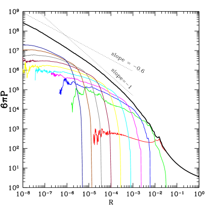
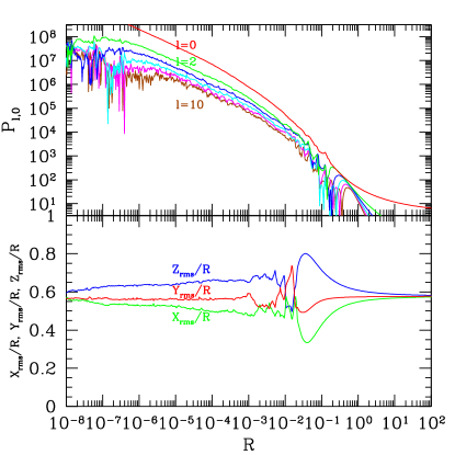
Figure 9 shows the angle-averaged density profiles for the solution with $\gamma=0.25$ and $e=0.1$. Comparing with the spherically symmetric case with the same $\gamma$ (Fig. 5) and with the axisymmetric case (Fig. 8), shows that the logarithmic slope of $P$ is much flatter for the 3D case, and nearly reaches the frozen slope $-g_{f}=-0.6$ at very small $R$. The spherically symmetric case has $g=2$ because its interior density field is dominated by particles that have recently collapsed and themselves lay down a shell profile with logarithmic slope -2. By contrast, in the triaxial case the recently collapsed shells have flatter tails. Physically, this is because non-radial motions prevent recently collapsed particles from penetrating the origin, whereas in the spherical case all particles are forced to go through the origin every orbital time (White & Zaritsky, 1992; Nusser, 2001). From Figure 9, it is apparent that the density field at increasingly small $R$ is dominated by particles with increasingly small $M_{i}$. This is in contrast to the spherical $\gamma=0.25$ case (Fig. 5) and to the axisymmetric $\gamma=0.25$ case (Fig. 8), but similar to the spherical $\gamma=2.5$ case (Fig. 2).

A surprising aspect of Figure 9 is how many decades in $R$ it takes the total density to roll over towards the frozen slope. Indeed, the slope has not yet reached $-g_{f}$ even at $R\sim 10^{-7}$, which is $\gtrsim 10^{5}$ times smaller than the virial radius. For $R$ smaller than that, it appears to reach $-g_{f}$, but the simulation has likely not converged at such small $R$. We shall discuss the reasons for the gradual roll-over of the slope below.

Figure 10 shows some higher order multipoles in the same solution as in Figure 9, quantifying the deviation from spherical symmetry. At a given $R$, the mass weighted r.m.s. co-ordinates differ from each other by around $30\%$.

Figure 11.— Density Profiles ($\gamma=0.25$, various values of $e$): The density profiles (top panel) have been compensated by $R^{g_{f}}$ to highlight their approach to the frozen slope at small $R$. The bottom panel shows the logarithmic slopes of the densities in the top panel. The frozen slope is $-g_{f}=-0.6$, indicated with a horizontal line.

Figure 12.— Density Profiles ($\gamma=1$, various values of $e$): similar to Fig. 11. The frozen slope is -1.5 at this $\gamma$.

Figure 13.— Density Profiles ($e=0.1$, various values of $\gamma$): Simulations with smaller $\gamma$ reach smaller asymptotic slopes. The $x-$axis has been rescaled by the $\delta_{c}^{1/\gamma}$ to roughly line up the virial radii of the various simulations, where $\delta_{c}\equiv 1.686$ is the critical density for top-hat collapse

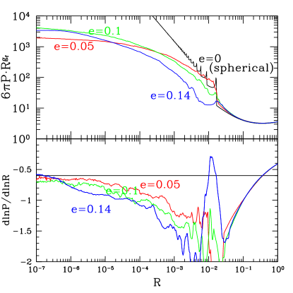
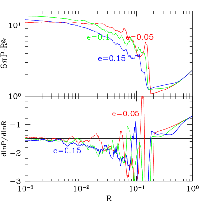
Figures 11-12 show the spherically-averaged density profiles for a number of solutions with various values of $e$ (and $p=0$), and with $\gamma=0.25$ and 1, respectively. In the top panels, the profiles have been multiplied by $R^{g_{f}}$ to show more clearly where they reach the frozen slope. The bottom panels show the logarithmic density slopes. For the triaxial simulations, increasing $e$ at fixed $\gamma$ tends to makes the profiles steeper, i.e. more discrepant with the frozen slope, and extends the range in $R$ over which the slope rolls over towards the frozen slope. It appears that all profiles do reach the frozen slope at small $R$. At larger $R$, increasing $e$ tends to spread out the outermost caustics, and pushes the rise in density below the caustic region to smaller radii.

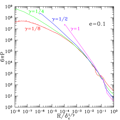
Figure 13 shows a set of solutions with $e=0.1$ and varying $\gamma$. Note that the $x-$axis has been rescaled to roughly line up the virial radii. Decreasing $\gamma$ tends to decrease the asymptotic slope at small $R$.

6.2. Caustics

Figure 14.— Caustics ($\gamma=0.25$): For the $e=0.05$ case (left), the top panel shows the scaled co-ordinates of the three axis particles. The bottom panel shows the density profile. Vertical lines are drawn where the three axis particles reach their first respective apoapses, in scaled co-ordinates. These locations correspond to the sharp rise in the density profile in the bottom panel. For the $e=0.14$ case (right), the time at which the long-axis particle ($Z$) hits its first scaled apoapse is significantly delayed relative to the short-axis particle ($X$). This is reflected in the density profile (bottom panel) by an extended flat region, and then a rise in density below $R\sim 0.004$, which is where the long-axis particle hits its first scaled apoapse.

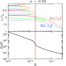
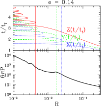
The density profiles of spherically symmetric solutions exhibit sharp spikes that are especially prominent at large radii (e.g., Fig. 2). These caustics occur near a particle’s apoapse, where its speed vanishes (Fillmore & Goldreich, 1984; Bertschinger, 1985). For triaxial halos, caustics are largely washed out in the spherically averaged density profiles (Fig. 11), because particles with different initial angular positions reach their apoapses at different radii and times.

In Figure 14 we examine caustics in more detail for two simulations, one with $e=0.05$ and the other with $e=0.14$. The bottom panel of the $e=0.05$ case shows a zoom-in of the density profile. Although most of the caustics present in the spherical run are washed out, similar to the results of Vogelsberger et al. (2010), there is a clear rise in density at $R\sim 0.02$, which is where the spherical run exhibits its first caustic (Fig. 11). The top panel shows the trajectories of the three axis particles; these are the particles that lie along the principal axes of the linear density field. For example, for the particle on the $z$-axis (which we take to be the long axis), the self-similar solution determines $Z(s)$, i.e. the $z$-component of $\mbox{\boldmath$R$\unboldmath}(s)$. In the top panel, the solid red line shows this $Z$ as the abscissa, and the time as the ordinate, where the time is converted from $s$ to $t/t_{f}$ via equation (29). Similarly, the blue and green curves show the particles that lie along the two shorter principal axes. At early times, towards the bottom of the panel, all three particles expand with the Hubble flow, and their scaled radii $X,Y,Z$ decrease together. Then, at $t/t_{f}\sim 1.8$ the particle along the short axis collapses and crosses through $X=0$. We emphasize that Figure 14 depicts scaled (i.e. self-similar) co-ordinates. When $X$ crosses through 0, the unscaled $x$ has already been through turnaround. This is not evident in the figure because $X$ decreases uniformly until it reaches the origin. As a result, the time and location of turnaround have only a small influence on the density profile. At $t/t_{f}\sim 2$, the short axis particle reaches its first scaled apoapse. This is close to when the unscaled $x$ reaches its first apoapse after turnaround. The long axis particle, labelled $Z$, reaches its first apoapse in scaled co-ordinates shortly after the short axis particle, and at nearly the same scaled radius. We also plot vertical lines at the locations of the first (scaled) apoapses, and extend them to the bottom panel, showing that the sharp rise in density is caused by the corresponding caustics.

The right half of the figure shows a similar plot, but with $e$ increased to $0.14$. In the top panel, one sees that the first scaled apoapse of the long-axis particle occurs significantly after that of the short-axis particle. Because of this, the former is significantly smaller than the latter, a somewhat counterintuitive result. This behavior is reflected in the density profile shown in the lower panel. At the location of the caustic of the short-axis particle, there is a modest rise in density. The density does not change significantly until reaching a much smaller radius ($R\sim 0.005$), close to where the long-axis particle reaches its first scaled apoapse.

6.3. Adiabatic Shrinking

Figure 15.— Root-mean-square co-ordinates of the set of particles that initially lie in the same spherical shell ($\gamma=0.25$ and $e=0.1$). The top panel shows the scaled r.m.s. co-ordinates, and the bottom panel the unscaled (i.e. proper) ones. There is much less shrinking at late times than in the spherical case (Fig. 7).

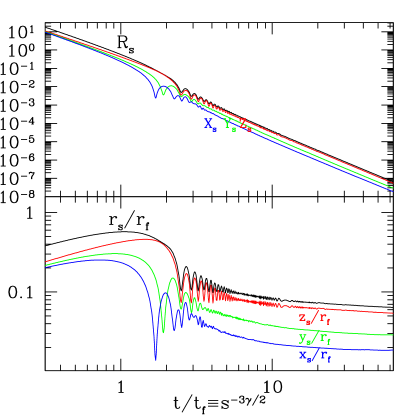
Figure 15 shows the time evolution of an initially thin spherical shell of particles in the $\gamma=0.25$, $e=0.1$ solution. In the top panel, we plot the r.m.s. value of $R$ for all particles that have the same $s$. We also show the r.m.s. values of the $X$, $Y$, and $Z$ co-ordinates for these particles. In the bottom panel, we convert the scaled co-ordinates of the top panel to unscaled ones (via eqs. [8] and [29]). At early times, the r.m.s. co-ordinates expand with the Hubble flow, until first the small axis ($x_{s}$) turns around and collapses, then the middle, and finally the long axis. At late times the axes continue to shrink, but by a much smaller amount than in the spherical simulation (Fig. 7). Eventually, the axes become nearly constant. This explains why the slope of the density profile reaches the frozen slope at very small radii (see point 2 above §3.1). Note also that at late times, the r.m.s. co-ordinates are in the ratio $3.1:1.6:1$.

6.3.1 Effect of shrinking on density profile

Figure 16.— Effect of shrinking on density profile ($\gamma=0.25$, $e=0.1$): The top panel shows the shell densities and total density, multiplied by the frozen profile $R^{g_{f}}$. The middle panel takes the shell profiles from the top panel, and “unshrinks” them; see text for details. The brown dotted line shows the sum of the shifted profiles. The profiles in the middle panel have also been compensated by $R^{g_{f}}$. The bottom panel shows the logarithmic slope of the total densities in the top two panels, showing that the shifted profile is much closer to the frozen one, with logarithmic slope much closer to $-g_{f}=-0.6$.

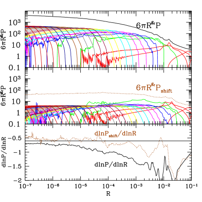
Surprisingly, the small amount of shrinking at late times has a marked effect on the slope of the density profile. Figure 16 illustrates this. The top panel of Figure 16 shows the density and shell profiles of the $e=0.1$, $\gamma=0.25$ solution, compensated by the frozen slope. Note that twice as many shells have been plotted in this panel as in Figure 9, each shell being half as wide logarithmically. In the middle panel, we spatially expand each shell profile from the top panel, conserving mass, such that the r.m.s. unscaled radii do not shrink; i.e., we set $P_{\rm shifted\ shell}(R)=c^{3}P_{\rm shell}(cR)$, where the factor $c$ was chosen to make the r.m.s. unscaled radius of each shifted shell equal to $r_{s}=0.5r_{f}$ (rather than declining in time, as seen in Fig. 15). The brown dotted line in the middle panel shows the sum of these shifted shell profiles. The bottom panel of the figure shows the logarithmic derivatives of the unshifted and shifted densities, showing that the latter is much closer to the frozen profile. This figure illustrates that the late-time shrinking of the r.m.s. radii plays a large role in causing the density profile to deviate from the frozen profile.

To see why the small amount of shrinking shown in Figure 15 leads to such a significant change in the density profile, we construct a simple model, which is a slight extension of the frozen model (§3). After each particle crosses $r_{*}$, we now allow its proper radius to decrease in time as a power-law, i.e. we set

$$r=r_{f}\left({t\over t_{f}}\right)^{-\beta},\ {\rm for\ }t>t_{f}$$ (37)

and ask what the resulting density profile would be. Dividing through by $r_{*}$ and using equations (11) and (29), we find $M_{i}={2\over 9}R^{3/(1+\gamma+3\beta\gamma/2)}$. Since in this model we ignore the post-collapse orbital motion (i.e. we take the shell profiles to be delta functions), we have $M_{i}=M$, implying that $P\propto R^{-g}$ at small $R$, where

$$g=3\gamma{1+3\beta/2\over 1+\gamma+3\beta\gamma/2}\approx g_{f}\left(1+{3\beta/2\over 1+\gamma}\right)\ ;$$ (38)

the approximation holds when $\beta\ll 1$. So if $\beta\sim 0.1$, it would lead to a $\sim 15\%$ deviation in the slope from the frozen slope. For example Figure 15 implies that at time $t/t_{f}=30$ (when $R_{s}\simeq 10^{-6}$) that $\beta\simeq 0.13$, and hence the above equation yields $g\simeq 0.7$. Comparing with the lower panel of Figure 16, we see that indeed the black line is nearly equal to $-0.7$ at $R\simeq 10^{-6}$.

6.3.2 Effect of density profile on shrinking

Figure 17.— Effect of density profile on shrinking: These plots show that shells shrink in inverse proportion to the average enclosed mass (eq. [39]). See text for details. The order-unity constant $k$ appearing in equation (39) was chosen to be 0.8 for the $\gamma=0.25$ simulations, and $0.4$ for the $\gamma=1$ simulation.

In spherically symmetric solutions, the apoapse of a particle shrinks in inverse proportion to the enclosed mass (eq. [33]). We show here that this is nearly true in 3D as well, even though the radial adiabatic invariant need not be conserved in the absence of spherical symmetry. To show this, we note that if the radius shrinks in inverse proportion to the enclosed mass, then

$$m(r)r={\rm const}=km_{i}r_{f}\ ,$$ (39)

where we write the constant as a product of three factors: the frozen radius $r_{f}$ (eq. [29]), the initial enclosed mass (see above eq. [11]), and an order unity constant $k$. Dividing through by $r_{*}^{4}/t^{2}$ yields the scaled equation

$$M(R)R={2\over 9}ks^{4+\gamma}\ .$$ (40)

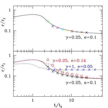
Hence the total enclosed mass profile $M(R)$ predicts how the radius of a shell decreases with decreasing $s$. The solid line in the top panel of Figure 17 shows the $M(R)R$ profile for the $\gamma=0.25$, $e=0.1$ simulation, where $M(R)$ is the angle-averaged enclosed mass profile (eq. [32]) that comes from the density profile shown in Figure 9. The colored points show, for each of the shell profiles in Figure 9, the r.m.s. value of $R$ as the abscissa, and $(2/9)ks^{4+\gamma}$ as the ordinate, where we select $k=0.8$ to fit the $M(R)R$ curve. From the fact that the points lie on top of the curve shows that equation (40) (and hence eq. [39]) is a good prescription for how the r.m.s. radii of the shells shrink in time. By contrast, if the shells did not shrink (i.e. if $r=k^{\prime}r_{f}$), they would have their r.m.s. $R_{s}\propto s^{1+\gamma}$, which would give the dotted line in Figure 17, with slope $(4+\gamma)/(1+\gamma)=17/5$. The middle panel of Figure 17 shows the same data as that in the top panel, but converted to unscaled radius and time, i.e. the $M(R)R$ profile has been converted to $s(R)$ via equation (40), and then the $R$ and $s$ have been converted to $r$ and $t$ via equation (29). The points show the r.m.s. radii of shells, and are identical to the black curve of Figure 15, lower panel, except that here we average over a wider range in $s$. This middle panel shows directly that the shrinking is due to the increase of enclosed mass. The bottom panel of Figure 17 repeats the data in the middle panel, and also shows two other simulations, showing that in all cases the shrinking is described quite well by equation (39).

Figure 18.— Trajectories of three randomly selected particles ($\gamma=0.25$, $e=0.1$): For each particle, the left column shows its co-ordinates, normalized to the frozen radius $r_{f}$; the right column shows the product of its co-ordinates with the corresponding speed, appropriately normalized, as well as the sum of the three ($r\cdot v$). The envelope of $r\cdot v$ is nearly constant, even at rather early times, indicating that the radial adiabatic invariant is nearly constant for each particle.

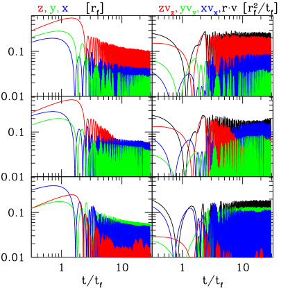
The fact that the radius decreases in inverse proportion to the enclosed massed is surprising, since for nonspherical potentials the radial adiabatic invariant need not be constant. And halos deviate significantly from spherical symmetry: at fixed $R$, the mass-weighted co-ordinates differ from each other by $\sim 30\%$ for the $e=0.1$ case (Fig. 10), and by $\sim 50\%$ for the $e=0.14$ case. Figure 18 exhibits an even more striking result: that the radial adiabatic invariant of individual particles is nearly constant. For that figure, we randomly selected three particles in the $\gamma=0.25$, $e=0.1$ simulation. (All other particles that we examined display similar behavior.) The three left panels show the unscaled co-ordinates of those three particles. And the right panels show the corresponding values of the co-ordinates multiplied by the respective co-ordinate speed. From the fact that the product $\mbox{\boldmath$r\cdot v$\unboldmath}=rv_{r}$ has a nearly constant envelope, we conclude that the radial adiabatic invariant $\propto\oint v_{r}dr$ is very nearly constant.

6.4. Shell Profiles

Figure 19.— Effect of the shell tails on the density profile ($\gamma=0.25$, $e=0.1$): The top panel shows the shell profiles from Figure 16, but truncated below $R_{s}/15$, where $R_{s}$ is the r.m.s. radius of each shell. The dotted magenta line is the sum of the truncated profiles, which deviates slightly from the untruncated profile (black line). All profiles are compensated by $R^{g_{f}}$. The middle panel is the same, except truncated below $R_{s}/1.5$. The bottom panel shows the logarithmic derivatives of the total density profiles from the top two panels.

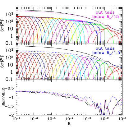
The tails of the shell profiles extend many orders of magnitude in radius (Fig. 16). How important are these tails for the shape of the total density profile? The top panel of Figure 19 shows the density profile that results from truncating the tails of the shell profiles below $R_{s}/15$, where $R_{s}$ is the r.m.s. radius of a shell. Specifically, for each shell profile shown in Figure 16, we compute the enclosed mass profile, and then multiply it by $x^{5}/(1+x^{5})$, where $x\equiv R_{s}/15$. The resulting density profiles are shown, as well as their sum, which is plotted as a magenta dotted line. The black line is the total (untruncated) profile. The middle panel is similar, except the shell profiles are truncated below $R_{s}/1.5$. The bottom panel shows the logarithmic derivatives of the total density profiles from the top two panels. We conclude that the deep tails of the shell profiles ($\lesssim R_{s}/15$), have little effect on the total density. But the moderately deep tails have a noticeable impact, particularly for $R\gtrsim 10^{-4}$, where the adiabatic shrinking is insufficient to account for the total deviation from the frozen slope (Fig. 16).

Therefore both effects—shell tails and the adiabatic shrinkage—influence the total density profile. Of course, our distinction between these two effects is somewhat artificial. It is the shell tails that increase the enclosed mass, which in turn causes adiabatic shrinkage. In the absence of shell tails there could be no adiabatic shrinking, because the mass enclosed by any shell would not change in time. We construct a toy model that incorporates both effects self-consistently below (§7).

Figure 20.— Normalized Shell Profiles ($\gamma=0.25$, $e=0.1$): The top panel shows 16 shell profiles from Figure 16’s top panel, but plotted here as enclosed mass rather than density, and with the mass and radius normalized by $M_{s}$ and $R_{s}$ (mass in the shell and r.m.s. radius of shell). From the fact that all of the shell profiles lie nearly on top of each other, we conclude that there is little evolution of the shell profile. The bottom panel shows the logarithmic derivatives of the profiles in the top panel. The vertical lines are the r.m.s. co-ordinates relative to $R_{s}$ multiplied by $\sqrt{5}$, as would be applicable for a constant density ellipsoid.

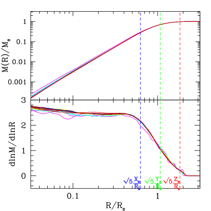
Figure 20 shows many of the shells from Figure 16, but replotted with a common normalization. Specifically, we take the 16 shells with $4.3\leq t/t_{f}\leq 36$, where the lower limit is the first magenta shell at large $R$, and the upper limit is, continuing to smaller $R$, the second red shell. For each shell, we plot in the top panel of Figure 20 its enclosed mass normalized to the total mass in the shell, versus its radius normalized to its r.m.s. radius. All 16 shells lie virtually on top of one another, implying that the shell profile hardly evolves in time. However, the profiles that we do not plot do show some evolution. Those at larger radii evolve as they virialize, and those at smaller radii are affected by the finite resolution of the simulation. The bottom panel of Figure 20 shows the slopes of the profiles in the top panels.

An important question remains: what sets the shell profile shape? Since the scaled shell profile is nearly time-invariant (Fig. 20), and since the scale itself is determined by adiabatic shrinking (§6.3), if one could predict the scaled profile just after collapse, one could then predict from first principles the total density profile of the self-similar solution. (In §7 we show how to compute the total density profile given the shell profile shape.) We discuss here our preliminary exploration of this question, leaving more detailed work to the future.

A simplistic assumption, useful as a baseline for comparison, is to suppose that the shell profile is similar to that of a constant density ellipsoid. This might be the case if particle orbits become highly chaotic after collapse, and if the particles from each shell uniformly fill an ellipsoidal volume. A constant density ellipsoid with semi-axes $a\gg b\gg c$ has an enclosed mass profile given by

$${d\ln M\over d\ln R}=\cases{0,&for $R\gg a$\cr 1,&for $a\gg R\gg b$\cr 2,&for $b\gg R\gg c$\cr 3,&for $c\gg R$}$$ (41)

On the smallest lengthscales ($c\gg R$), the enclosed mass increases as the volume enclosed by a sphere of radius $R$, i.e. $M\propto R^{3}$. For comparison, we argued above that in spherically symmetric collapse the shell profile at small $R$ scales as $M\propto R$ (§4.2), and that in axisymmetric collapse $M\propto R^{2}$ (§5). By reasoning similar to that presented in §5, one would conclude that in the triaxial case the shell profile should scale as $M\propto R^{3}$ for $R\rightarrow 0$ if particles uniformly explore a region in three dimensions. For a constant density ellipsoid, on scales larger than $c$ the enclosed mass increases less and less rapidly with $R$ as $R$ crosses the semi-major axes of the ellipsoid, until at the largest radii the ellipsoid contributes no more mass, and hence $M\propto R^{0}$.

In Figure 20 as well, one can see that the logarithmic slope of $M$ rolls over from 0 at large radii, to (nearly) 3 at small radii. The vertical dashed lines show the ratio of the r.m.s. co-ordinates to $R_{s}$, multiplied by $\sqrt{5}$; that factor is to account for the fact that a constant density ellipsoid has r.m.s. co-ordinates equal to $1/\sqrt{5}$ times its semi-axes. Hence the profile is broadly similar to that of a constant densitiy ellipsoid, with the features in $d\ln M/d\ln R$ corresponding to the r.m.s. co-ordinates. Nonetheless, there are a number of differences, as discussed below.

Figure 21.— Triaxiality of Shell Profiles ($\gamma=0.25$, $e=0.1$): For each of the shell profiles from Figure 20, we plot the r.m.s. co-ordinates of particles that have the same $R$. At large radii, most of the particles lie near the $z$-axis, while at small radii, the r.m.s. co-ordinates are nearly isotropic. This behavior is similar to that of a constant density triaxial ellipsoid with semi-axes $\sqrt{5}X_{s}$, $\sqrt{5}Y_{s}$, and $\sqrt{5}Z_{s}$.

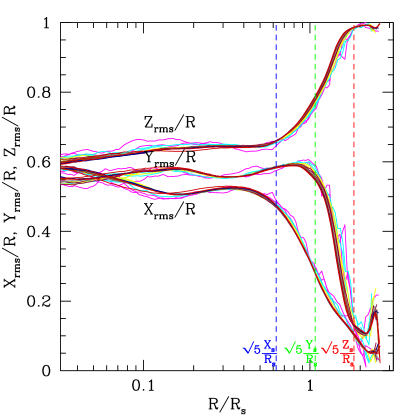
Figure 21 shows directly the triaxiality of the shell profiles. For each shell profile, we plot the r.m.s. co-ordinates of particles with the same $R$. At large $R/R_{s}$ most particles lie along the $z$-axis. Proceeding to smaller $R/R_{s}$, particles first approach isotropy in the $y$ and $z$ directions, and then in all three directions. At small radii, the three r.m.s. co-ordinates approach $R/\sqrt{3}=0.577R$, corresponding to isotropy in all three directions. This behavior is similar to that of a constant density triaxial ellipsoid.

While Figures 20-21 indicate that the shell profile is roughly consistent with that of a constant density ellipsoid, the agreement is not perfect. For example, the slope $d\ln M/d\ln R$ does not quite reach 3 until very small $R$. The reason for this appears to be that particles that initially lie near the $z$-axis (i.e., the eventual long axis of the ellipsoid) collapse more in the transverse ($x-y$ dimension) than those that lie further from the $z$-axis. Therefore, the collapsed ellipsoid is in fact more centrally concentrated than a constant density ellipsoid. However, quantifying this effect remains a topic for future work. Nonetheless, we recall that the deep shell profile (at $R\ll R_{s}$) has little effect on the final density profile (Fig. 19). Hence it is possible that the details of this extra concentration are of little importance for the total density profile.

It is instructive to compare our shell profiles with those predicted from spherical self-similar models that include non-radial motions (e.g., Nusser, 2001; Lu et al., 2006; Del Popolo, 2009; Zukin & Bertschinger, 2010). In the simplest of these models, particles are assigned a constant angular momentum (in scaled units) at turnaround. Therefore the shell profile is similar to the spherical solution outside of periapse, i.e. $M(R)\propto R$, for $R_{\rm peri}<R<R_{\rm apo}$, and $M=0$ for other values of $R$. This profile differs from that of Figure 20 where the slope of $d\ln M/d\ln R$ gradually rolls over. More sophisticated spherical infall models have been proposed that, for example, assign a distribution of angular momenta at turnaround (Lu et al., 2006) or that vary the angular momentum after turnaround based on a prescription motivated by tidal torque theory (Zukin & Bertschinger, 2010). One could in principal assign the angular momenta (or equivalently the periapses) in such models in such a way to mimic our Figure 20, or indeed any shell profile shape. Nonetheless, it does not appear that such models adequately explain our results, for at least two reasons. First, when we examine the angular momenta of individual particles in our solutions, we find that they vary substantially—even over the course of a single orbit—because of the asphericity of the potential. By contrast, in spherical models the angular momenta are constant (aside from externally imposed changes). In fact, the majority of orbits in our solutions appear to be more box-like than loop-like. This leads us to suppose that our model based on a homogeneous ellipsoid is more appropriate than spherical models that are based on angular momentum conservation. And second, it is evident from Figure 21 that triaxiality is playing a leading role in the range of radii where $d\ln M/d\ln R$ rolls over, whereas in the spherical models, all three r.m.s. axes would be equal to $0.577R$. Nonetheless, our explorations at this stage are preliminary; more self-similar solutions should be examined, and in more detail, before definitive statements can be made regarding what sets the shell profiles.

7. Toy Model

We have shown that two effects are largely responsible for the total density profile: adiabatic shrinking and the shape of the shell profiles. Here we construct a simple toy model that incorporates both effects, similar to the models of Lu et al. (2006); Del Popolo (2009) . We assume that after a shell collapses it has a (scaled) outer radius $R_{\rm shell}(s)$, and that its shell profile is time-invariant when scaled to $R_{\rm shell}$. This is roughly true of the shell profiles seen in the full simulations. We define $M_{\rm shells}(R)$ to be the total (scaled) mass from all shells with $R_{\rm shell}<R$. Then the total enclosed (scaled) mass is

$$M(R)=M_{\rm shells}(R)+\int_{R}^{1}{dM_{\rm shells}\over dR^{\prime}}\mu(R/R^{\prime})dR^{\prime}\ ,$$ (42)

where $\mu(R/R^{\prime})$ is the shell mass profile, i.e. the fraction of mass that a shell with outer radius $R^{\prime}$ contributes to a sphere of radius $R$, where $R<R^{\prime}$. Our assumption that the shell profile is invariant when scaled to its outer radius dictates that $\mu$ is a function only of the ratio $R/R^{\prime}$; note that $\mu(R/R^{\prime})\leq 1$, with equality holding at $R/R^{\prime}=1$. Our second assumption is that a shell’s proper outer radius shrinks adiabatically in inverse proportion to the enclosed mass, i.e.

$$RM=M_{\rm shells}^{(4+\gamma)/3}$$ (43)

(eqs. [11] and [40]). Equations (42)-(43) are the toy model equations. We drop order-unity constants in these equations, which corresponds to setting $R=1$ at the outer-most radius, i.e., the radius at which $M=M_{\rm shells}$. The equations may be solved upon specification of the shell profile function $\mu()$. In fact, when

$$\mu(R/R^{\prime})=\left(R/R^{\prime}\right)^{\eta}\ ,$$ (44)

they may be solved analytically, after re-writing equation (42) as $dM/dR=(\eta/R)(M-M_{\rm shells})$, and then inserting equation (43).

Figure 22.— Toy Model ($\gamma=0.25$): The top panel shows the compensated density profiles that result from solving the toy model equations (eqs. [42]-[43]). The lower panel shows the logarithmic slopes. The black solid line is for $\eta=1$ in equation (44), corresponding to the shell profiles of the spherically symmetric solution that have density $\propto R^{-2}$. The resulting density profile is also $\propto R^{-2}$. The blue dashed line is for $\eta=3$, corresponding to a constant density sphere. This is the minimal tail expected, and leads to a total density profile that rolls over to the frozen slope over an extended range in $R$. The red dashed line is for a shell profile that transitions from $\eta=1$ at large $R/R^{\prime}$ to $\eta=3$ below $R/R^{\prime}=1/3$. The resulting total profile is similar to that seen in the full simulation (Fig. 16).

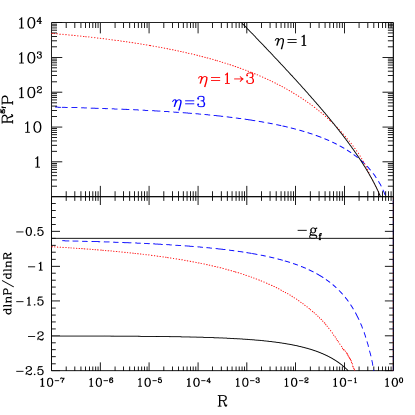
Figure 22 shows the solution for three possible shell profiles, when $\gamma=0.25$. The upper panel shows the total density profiles (compensated by the frozen slope), and the lower panel shows their logarithmic derivatives. The blue dashed curve is the result when $\mu=(R/R^{\prime})^{3}$. This form for $\mu$ would result from a constant density sphere. It is the minimal “tail” expected, since realistic tails tend to be more centrally concentrated. One might have expected that the density in this minimal tail model would reach the frozen slope fairly quickly. But in fact it takes over 5 decades in $R$ to roll over; nonetheless, it does roll over faster than the actual solutions (e.g., Fig. 16). The black solid line in Figure 22 shows the result when $\mu=(R/R^{\prime})$. This corresponds to the spherical case, where the shell density profiles are proportional to $1/R^{2}$ (§4). Since in this case the shell density profiles are steeper than the frozen slope $g_{f}=0.6$, the total density profile asymptotes to that of an individual shell, i.e. to a logarithmic slope of -2. The red dotted curve shows the result of setting $\mu$ to be a broken power-law, with $\mu\propto(R/R^{\prime})$ at large radii $(1/3<R/R^{\prime}<1)$, and $\mu\propto(R/R^{\prime})^{3}$ at small radii $(R/R^{\prime}<1/3)$. This form was chosen as a rough model for the shell profiles in Figure 16 (see also Fig. 20). The resulting density profile is quite similar in form to that seen in the full simulation of Figure 16.

In the latter broken power-law model, the roll-over in the shell profile extends for only half a decade in $R$. Yet the resulting roll-over in the total density profile extends over five decades in $R$. Recalling that the outer shell profile controls the total density profile in the self-similar solutions (Fig. 19), and that the outer shell profile is in turn largely controlled by the ellipticity of collapsed shells (Figs. 20 and 21), we therefore attribute the extended roll-over of the total density profiles largely to the ellipticity of collapsed shells. Our picture therefore differs from that of spherical infall models with non-radial velocities (e.g., Zukin & Bertschinger, 2010), where it is the distribution of periapses that controls the shell profile, and hence the total density profile (see also §6.4). Our picture suggests an explanation for why increasing $e$ (the ellipticity of the linear density field) extends the range in $R$ over which the slope rolls over towards the frozen slope, as shown in Figures 11-12. Increasing $e$ makes collapsed shells more elliptical. This extends the rollover in the shell profile, which in turn extends the rollover of the total density profile.

8. Summary and Discussion

We constructed self-similar solutions that describe the formation, virialization, and growth of dark matter halos in three dimensions. As long as the initial linear density perturbation in a flat CDM Universe can be written as $\delta_{\rm lin}\propto r^{-\gamma}f(\theta,\phi)$, the subsequent evolution is described by the self-similar equations (eqs. [13], [18], and [21]), subject to no approximation. In §A, we detailed the algorithms we developed to solve these equations numerically. Our solutions are the natural extension of the spherically symmetric solutions of Fillmore & Goldreich (1984) and Bertschinger (1985), and of the axisymmetric solutions of Ryden (1993), to the case without any assumed angular symmetry. Whereas other authors have considered 3D solutions by modelling the effects of angular momentum, our approach differs, in that we solve the full equations of motion. This leads to more complicated solutions, but ones that are physically realistic.

Even though our assumed form for $\delta_{\rm lin}$ is idealized, the subsequent self-similar evolution can be studied in great detail. Significantly higher radial resolution can be achieved than with N-body simulations. For example, Figure 9 extends to below $\sim 10^{-5}$ of the virial radius, whereas the highest resolution N-body simulations reach $\sim 0.004$ of the virial radius (e.g., Navarro et al., 2010). Furthermore, for any assumed $\gamma$ and angular function $f(\theta,\phi)$, there is a well-defined solution, which can be approached with simulations of ever increasing accuracy. By contrast, cosmological N-body simulations are initialized with random fields, and this element of randomness complicates the analysis of the physical processes involved.

In this paper, we used the similarity solutions to explore the processes responsible for the density profile. In §3, we introduced the frozen model, in which particles freeze when they reach the radius of nonlinearity, $r_{*}$. This is not meant as a physical model, but merely to help in the analysis of the full nonlinear solutions. In §4, we reviewed the well-known spherical solutions, focusing on the processes important for the density profile: adiabatic contraction and shell profiles, i.e. the density profile laid down by the set of particles that occupy the same thin spherical shell at early times. In §5, we showed that axisymmetric solutions always have interior logarithmic slope $\leq-1$. But even though this is suggestive of NFW, real halos are not axisymmetric but triaxial. In §6 we presented a suite of triaxial solutions, and analyzed them in considerable detail. We found that the shape of the density profile can be simply understood by decomposing it into its component shell profiles. Our principal results are as follows:

• The density profile rolls over to the frozen slope $-g_{f}$. But the roll-over can extend for many decades in radius.

• The reason for the extended roll-over can be attributed primarily to two effects: adiabatic shrinking and shell tails

• adiabatic shrinking: the r.m.s. radius of a collapsed shell decreases in inverse proportion to the enclosed mass (Fig. 17). A small amount of adiabatic shrinking can have a surprisingly large influence on the density profile (Fig. 16)

• shell tails: although the density profile of a collapsed shell extends for many orders of magnitude in radius, only the outermost decade or so affects the total density profile (Fig. 19). The triaxial shape of a collapsed shell is largely responsible for the shell profile in this range of radii (Fig. 20, bottom panel and Fig. 21). Furthermore, the shape of the shell profile shows little temporal evolution after virialization (Fig. 20, top panel).

In §7, we incorporated the above results into a toy model, and showed that when the shell profile was chosen to approximate that in the self-similar solution, the toy model roughly reproduced the self-similar solution’s total density profile.

The one element missing from our toy model is an estimate of the shell profile shape given the properties of the linear overdensity. This is a topic for future work.

In a companion paper (Dalal et al., 2010), we apply our understanding of what sets the density profiles in the self-similar solutions to realistic halos. For such halos, $\delta_{\rm lin}$ is a Gaussian random field, in which peaks are not scale-invariant and contain a hierarchy of peaks within peaks, leading to copious halo substructure. Despite these complications, we show that many aspects of halo structure in realistic hierarchical cosmologies may be understood using the relatively simple picture described here.

We anticipate that 3D self-similar solutions will be a helpful tool for exploring the physics of halo formation. Here we focused on the density profile. But the similarity solutions can also be used to explore other properties of halos, such as the velocity structure within halos, the orbital characteristics of collapsed particles, the phase space density, and the detailed structure of caustics. These remain topics for future work.

Appendix A

APPENDIX A: NUMERICAL SOLUTION OF THE SELF-SIMILAR EQUATIONS

In §2.2 we briefly describe how we solve the self-similar equations (eqs. [13], [18], and [21]). Here we provide more detail. As a check of our numerical implementation, we wrote two independent codes, one by each author; one code employs spherical harmonics for the angular dependences of the fields, and the other employs a $\theta-\phi$ grid. We focus first on the former code, and then describe the principle differences of the latter.

In the spherical harmonic code, the density is expanded as

$$P({\mbox{\boldmath$R$\unboldmath}})=\sum_{l,m}P_{lm}(R)Y_{lm}(\theta,\phi)\ ,$$ (A1)

and similarly for $\Phi({\mbox{\boldmath$R$\unboldmath}})$. We assume eightfold symmetry (i.e., $P(X,Y,Z)=P(-X,Y,Z)$ and similarly for $Y$ and $Z$), and hence include only terms with even $l$ and $m$, and $0\leq m\leq l_{\rm max}$. The functions $P_{lm}(R)$ and $\Phi_{lm}(R)$ are stored on a logarithmic grid in $R$, with around 100 gridpoints per decade in $R$, and a total extent of 10-20 decades.

For the first step of each iteration, $P$ is transformed into $\Phi$ by inverting Poisson’s equation (eq. [21]):

$$\Phi_{lm}(R)=-{4\pi\over 2l+1}\left({1\over R^{l+1}}\int_{0}^{R}P_{lm}(R^{\prime})R^{\prime l+2}dR^{\prime}+R^{l}\int_{R}^{\infty}P_{lm}(R^{\prime})R^{\prime-l+1}dR^{\prime}\right)\ .$$ (A2)

Since the second integral extends to infinity, the linear density field (eq. [22]) is used for the part of the integral that lies beyond the $R$-grid. For $l=0$, this integral can diverge, in which case an infinite constant may be added (which does not affect the equation of motion) by replacing the second term in parentheses with -$\int_{0}^{R}P_{lm}(R^{\prime})R^{\prime}dR^{\prime}$.

For the second step, particle trajectories are integrated in a fixed potential (eq. [13]), and their mass is accumulated into $P_{lm}(R)$. Particles are initialized at large $s$ where they nearly expand with the Hubble flow $({\mbox{\boldmath$R$\unboldmath}}\simeq{\mbox{\boldmath$s$\unboldmath}})$. Their directions are chosen to be uniformly spaced in $\cos\theta_{s}$ and $\phi_{s}$, where these angles refer to the direction of $s$, which differs from the direction of $R$ by a finite (but small) amount. Their initial $R$ is chosen to coincide with the last element of the $R$-grid. These constraints are satisfied to linear order by applying the linear solution (§B), in which the linear potential comes from the inverse Laplacian of the imposed linear density (eq. [22]). The linear solution is also used to set the initial velocity field. We employ around 400 particles in $\theta_{s}$ and 100 in $\phi_{s}$.

Particle orbits are integrated with 4th-order Runge-Kutta with adaptive stepping. The force ${\mbox{\boldmath$\nabla$\unboldmath}_{R}}\Phi$ is evaluated by spherical harmonic expansion. The required $\Phi_{lm}$’s are obtained by linearly interpolating from the grid and the $Y_{lm}$’s and their derivatives are evaluated at the particle’s angular position. Also needed are the $d\Phi_{lm}/dR$; for this purpose we compute a grid of $d\Phi_{lm}/dR$ at the start of each iteration step by evaluating the derivative of the right-hand side of equation (A2) on the $R$-grid.

At each $s$ step, the particle’s mass is deposited into $P_{lm}(R)$ according to equation (18). To be specific, when taking a step $ds$, the right-hand side of equation (18) implies that the particle should deposit the (scaled) mass $dM=s^{2}dsd\Omega_{s}/6\pi$ onto the grid, where $d\Omega_{s}=d\cos\theta_{s}d\phi_{s}=4\pi$/(no. of particles) is the solid angle subtended in $s$. Therefore this $dM$ is multiplied by the $Y_{lm}^{*}$’s at the angular position of the particle, and added into $P_{lm}$ (with the appropriate weighting for the size of the relevant $R$-grid element). To increase the accuracy of the mass deposition, we limit the stepsize $ds$ so that a particle does not change its $R$ by much more than the local grid spacing. In addition, whenever a particle crosses a gridpoint in $R$, we use linear interpolation to find where in $s$ it crossed the gridpoint, and split its deposited mass accordingly into the two grid bins. This is especially important during the linear phase of the evolution (at large $R$) where small errors in the total density produce large errors in the overdensity.

A particle’s integration is terminated when the value of $R$ at its last apoapse is comparable to the $R$ of the first grid element. Note that at late times apoapses typically remain constant or shrink in $r$ (i.e. in real, not scaled coordinates). Therefore, their $R$ decreases with decreasing $s$ in proportion to $s^{\gamma+1}$, or faster. Hence all particles eventually have apoapses with arbitrarily small $R$. In addition to this stopping criterion, we also occasionally limit $s$ to a minimum value, or limit the number of apoapses per particle.

The algorithm as described above is trivially parallelized. We have done this by allocating a subset of the particles to each processor. Each processor holds a copy of the $\Phi_{lm}$, and accumulates the $P_{lm}$ from its own particles. At the end of each iteration step, the $P_{lm}$ from the different processors are then combined and inverted to yield the $\Phi_{lm}$.

We have also written a second independent code to solve the self-similar equations, as a check of our numerical solutions. Both codes use similar particle integration schemes and radial resolution, but differ principally in the implementation of the force solver. Instead of computing spherical harmonic coefficients $P_{lm}$ directly from the particle data, our second code bins the density into a three-dimensional grid, in $\log R$, $\theta$ and $\phi$. Then, the spherical harmonic coefficients are computed using the fast transform library S2kit. We then solve for the potential $\Phi$ and its derivatives on the grid, using spherical harmonic transforms, and interpolate the force from the 3-D grid onto the particle positions as required for the orbit integrations.

Our discrete sampling of the initial phase space can lead to spurious high-$l$ power in the linear regime at large $R$. To suppress this effective shot noise, we use the high-order Triangle-Shaped Cloud interpolation (Hockney & Eastwood, 1988) for the angular grid, and simple linear interpolation in the radial direction. In addition, because the angular grid does not have a pixel at $\theta=0$, special care must be taken to handle particles passing near the pole. We keep an additional array storing the potential derivatives at $\theta=0$ for each radial bin, calculated analytically from the harmonic coefficients, and employ it in the force interpolation for particles traversing the smallest $\theta$ grid cells. The memory requirements of this code are minimal, and the inter-node communications are negligible, leading to efficient performance on essentially any architecture. For a typical run with $l_{\rm max}=28$, radial range of 16 decades in $R$, and ${\cal O}(10^{7})$ particles, each iteration requires roughly one hour on 60 nodes, and the solutions reach convergence in typically 5-10 iterations, though we usually ran 15 iterations to be assured of convergence.

Appendix B

APPENDIX B: LINEAR SOLUTION OF THE SELF-SIMILAR EQUATIONS

The self-similar equations ([13], [18], and [21]) have zeroth order solution (i.e., in the limit $R\rightarrow\infty$):

$${\mbox{\boldmath$R$\unboldmath}_{0}}={\mbox{\boldmath$s$\unboldmath}};\ {\mbox{\boldmath$V$\unboldmath}_{0}}={2\over 3}{\mbox{\boldmath$s$\unboldmath}};\ \Phi_{0}={1\over 9}R^{2};\ P_{0}={1\over 6\pi}\ .$$ (B1)

To linear order, we set

$$P_{1}(\mbox{\boldmath$R$\unboldmath})={1\over 6\pi}R^{-\gamma}f(\theta,\phi)\ ,$$ (B2)

where $f$ is arbitrary. The linear potential is

$$\Phi_{1}(\mbox{\boldmath$R$\unboldmath})=R^{2-\gamma}g(\theta,\phi)\ ,$$ (B3)

where $g$ may be found from $f$ by inverting Poisson’s equation (eq. [21]). Equation (13) is to linear order

$${d\over d\ln s}\left(\begin{array}[]{c}{\mbox{\boldmath$R$\unboldmath}_{1}}\\ {\mbox{\boldmath$V$\unboldmath}_{1}}\end{array}\right)=\left(\begin{array}[]{cc}\gamma+1&-{3\gamma\over 2}\\ {\gamma\over 3}&1-{\gamma\over 2}\end{array}\right)\left(\begin{array}[]{c}{\mbox{\boldmath$R$\unboldmath}_{1}}\\ {\mbox{\boldmath$V$\unboldmath}_{1}}\end{array}\right)+{3\gamma\over 2}\left(\begin{array}[]{c}0\\ {\mbox{\boldmath$\nabla$\unboldmath}_{s}\Phi_{1}}\end{array}\right)\ ,$$ (B4)

considering $\Phi_{1}$ to be a function of $s$ instead of $R$, which is valid to linear order. Because this is a linear equation, $\mbox{\boldmath$R_{1}$\unboldmath},\mbox{\boldmath$V_{1}$\unboldmath}$ must be constants times $\mbox{\boldmath$\nabla_{s}$\unboldmath}\Phi_{1}$, and hence they scale with $s$ as $s^{1-\gamma}$. Replacing ${d\over d\ln s}\rightarrow 1-\gamma$ gives

$$R_{1} = -{3\over 2}\mbox{\boldmath$\nabla_{s}$\unboldmath}\Phi_{1}$$ (B5)

$$V_{1} = -2\mbox{\boldmath$\nabla_{s}$\unboldmath}\Phi_{1}\ .$$ (B6)

The velocity relative to the local Hubble flow is $\mbox{\boldmath$V$\unboldmath}-2\mbox{\boldmath$R$\unboldmath}/3=-{\mbox{\boldmath$\nabla$\unboldmath}_{s}}\Phi_{1}$, a well-known result. The linearized equation describing mass deposition (eq. [18]),

$$6\pi P_{1}={d^{3}s\over d^{3}R}-1=-{\mbox{\boldmath$\nabla$\unboldmath}_{s}\cdot R_{1}(s)}={3\over 2}\nabla^{2}_{s}\Phi\ ,$$ (B7)

is equivalent to Poisson’s equation. The reason for this redundancy is that in writing equation (13) we already took into account the linear evolution in setting the form of $r_{*}$. One could alternatively set $r_{*}=t^{\alpha}$, with arbitrary $\alpha$; equation (B7) would then prove that $\alpha={2\over 3}+{2\over 3\gamma}$.

Appendix C

APPENDIX C: PARAMETERIZATION OF THE LINEAR DENSITY FIELD

We follow Bond & Myers (1996) in parameterizing the local tides near peaks using the ellipticity $e$ and prolateness $p$ of the tidal field, defined as follows. Let $\Phi$ be the peculiar gravitational potential smoothed on scale $R_{\rm smooth}$, and write $\{\lambda_{a}\},\ a=1,2,3$ as the eigenvalues of the tidal tensor $\nabla_{i}\nabla_{j}\Phi$, ordered such that $\lambda_{1}\leq\lambda_{2}\leq\lambda_{3}$. Note that the overdensity $\delta=\sum_{a}\lambda_{a}$. The ellipticity and prolateness are then defined as

$$e = \frac{\lambda_{3}-\lambda_{1}}{2\delta}$$ (C1)

$$p = \frac{\lambda_{3}-2\lambda_{2}+\lambda_{1}}{2\delta}.$$ (C2)

In general, $e$ and $p$ are explicit functions of the smoothing scale. For our scale-free initial profiles, however, the smoothing scale cancels, and $e$ and $p$ may be expressed in terms of the relative amplitudes of the $l=2$ multipoles compared to the monopole. If we write the linear density profile as

$$\rho(r,\theta,\phi)=r^{-\gamma}[1+a_{20}Y_{2,0}(\theta,\phi)+a_{22}(Y_{2,2}+Y_{2-2})]$$ (C3)

then we have

$$a_{20} = \sqrt{10\pi}(3e+p)\frac{\gamma}{3-\gamma}$$ (C4)

$$a_{22} = \sqrt{\frac{15\pi}{2}}(e-p)\frac{\gamma}{3-\gamma}$$ (C5)

References

- Ascasibar et al. (2004) Ascasibar, Y., Yepes, G., Gottlöber, S., & Müller, V. 2004, MNRAS, 352, 1109, arXiv:astro-ph/0312221
- Ascasibar et al. (2007) Ascasibar, Y., Hoffman, Y., & Gottlöber, S. 2007, MNRAS, 376, 393, arXiv:astro-ph/0609713
- Bardeen et al. (1986) Bardeen, J. M., Bond, J. R., Kaiser, N., & Szalay, A. S. 1986, ApJ, 304, 15
- Bertschinger (1985) Bertschinger, E. 1985, ApJS, 58, 39
- Bond & Myers (1996) Bond, J. R., & Myers, S. T. 1996, ApJS, 103, 1
- Dalal et al. (2010) Dalal, N., Lithwick, Y., & Kuhlen, M. 2010, ArXiv e-prints, 1010.2539
- Del Popolo (2009) Del Popolo, A. 2009, ApJ, 698, 2093, 0906.4447
- Diemand et al. (2007) Diemand, J., Kuhlen, M., & Madau, P. 2007, ApJ, 667, 859, arXiv:astro-ph/0703337
- Diemand et al. (2008) Diemand, J., Kuhlen, M., Madau, P., Zemp, M., Moore, B., Potter, D., & Stadel, J. 2008, Nature, 454, 735, 0805.1244
- Duffy & Sikivie (1984) Duffy, L. D., & Sikivie, P. 2008, Phys. Rev. D, 78, 063508
- Eisenstein & Loeb (1995) Eisenstein, D. J., & Loeb, A. 1995, ApJ, 439, 520
- Fillmore & Goldreich (1984) Fillmore, J. A., & Goldreich, P. 1984, ApJ, 281, 1
- Gao et al. (2008) Gao, L., Navarro, J. F., Cole, S., Frenk, C. S., White, S. D. M., Springel, V., Jenkins, A., & Neto, A. F. 2008, MNRAS, 387, 536, 0711.0746
- Hockney & Eastwood (1988) Hockney, R. W., & Eastwood, J. W. 1988, Computer simulation using particles (Bristol: Hilger)
- Lu et al. (2006) Lu, Y., Mo, H. J., Katz, N., & Weinberg, M. D. 2006, MNRAS, 368, 1931, arXiv:astro-ph/0508624
- Moore et al. (1998) Moore, B., Governato, F., Quinn, T., Stadel, J., & Lake, G. 1998, ApJ, 499, L5+, arXiv:astro-ph/9709051
- Navarro et al. (2010) Navarro, J. F. et al. 2010, MNRAS, 402, 21, 0810.1522
- Nusser (2001) Nusser, A. 2001, MNRAS, 325, 1397, arXiv:astro-ph/0008217
- Ryden (1993) Ryden, B. S. 1993, ApJ, 418, 4
- Ryden & Gunn (1987) Ryden, B. S., & Gunn, J. E. 1987, ApJ, 318, 15
- Stadel et al. (2009) Stadel, J., Potter, D., Moore, B., Diemand, J., Madau, P., Zemp, M., Kuhlen, M., & Quilis, V. 2009, MNRAS, 398, L21, 0808.2981
- Vogelsberger et al. (2010) Vogelsberger, M., Mohayaee, R., & White, S. D. M. 2010, ArXiv e-prints, 1007.4195
- White & Zaritsky (1992) White, S. D. M., & Zaritsky, D. 1992, ApJ, 394, 1
- Zukin & Bertschinger (2010) Zukin, P., & Bertschinger, E. 2010, ArXiv e-prints, 1008.0639