The Dark Side of QSO Formation at High Redshifts

Abstract

Observed high-redshift QSOs, at $z\sim 6$, may reside in massive dark matter (DM) halos of more than $10^{12}~{}M_{\odot}$ and are thus expected to be surrounded by overdense regions. In a series of 10 constrained simulations, we have tested the environment of such QSOs. The usage of Constrained Realizations has enabled us to address the issue of cosmic variance and to study the statistical properties of the QSO host halos. Comparing the computed overdensities with respect to the unconstrained simulations of regions empty of QSOs, assuming there is no bias between the DM and baryon distributions, and invoking an observationally-constrained duty-cycle for Lyman Break Galaxies, we have obtained the galaxy count number for the QSO environment. We find that a clear discrepancy exists between the computed and observed galaxy counts in the Kim et~al. (2009) samples. Our simulations predict that on average eight $z\sim 6$ galaxies per QSO field should have been observed, while Kim et~al. (2009) detect on average four galaxies per QSO field compared to an average of three galaxies in a control sample (GOODS fields). While we cannot rule out a small number statistics for the observed fields to high confidence, the discrepancy suggests that galaxy formation in the QSO neighborhood proceeds differently than in the field. We also find that QSO halos are the most massive of the simulated volume at $z\sim 6$ but this is no longer true at $z\sim 3$. This implies that QSO halos, even in the case they are the most massive ones at high redshifts, do not evolve into most massive galaxy clusters at $z=0$.

1. Introduction

QSOs are among the most luminous objects in the universe and can be detected at high redshifts, when the universe was still very young — so far up to $z\sim 6.42$ (e.g., Fan et~al., 2003; Willott et~al., 2010). The comoving space density at the bright end of the luminosity function (as detected by the Sloan Digital Survey, SDSS York et~al., 2000) is $\sim(2.2\pm 0.73)~{}h^{3}\mathrm{Gpc}^{-3}$ at $z\sim 6$ (Fan et~al., 2004). Observations of high-$z$ QSOs raise a number of fundamental questions: where and how they formed, and what is their relationship to the formation of first stars and galaxies in the universe. High-$z$ QSOs are important cosmological probes for studying the star formation history, metal enrichment, early galaxy formation, growth of supermassive black holes (SBHs), properties of the interstellar and intergalactic matter, and the epoch of re-ionization in the universe.

Rare, high-$z$ QSOs have been claimed to form in highly overdense regions of the initial matter distribution. Their central SBHs are expected to have grown fast via mergers and/or accretion. Observed QSOs at $z\sim 6$ appear to host SBHs of $\sim 10^{9}M_{\odot}$ possibly residing within the most massive halos of a few $\times 10^{12}M_{\odot}$. Numerical simulations estimate a similar (to high-$z$ QSOs) comoving density $\sim$ 1 Gpc^-3 of these massive halos (e.g., Springel et~al., 2005; Sijacki et~al., 2009). This similarity however, depends on the so-called QSO duty cycle, or a fraction of the time the QSO is actually active. If this duty cycle is less than unity, the QSOs are less rare and correspondingly reside in the less massive halos (e.g., Overzier et al. 2009). Additional arguments have been used in favor of high-$z$ QSOs residing in lower mass halos (e.g., Willott et al. 2005).

Kaiser (1984) and Efstathiou & Rees (1988) have shown that the presence of high peaks (rich clusters) in the primordial density field enhances their correlation function. Compared to clusters, galaxies have a smaller correlation length $\xi(r)=1$ for $r_{g}\approx 4-7~{}h^{-1}\mathrm{Mpc}$ (Davis & Peebles, 1983). Therefore, primordial galaxy-size high peaks could in principle increase the clustering of galactic mass-scale halos in their vicinity (Muñoz & Loeb, 2008).

Population of galaxies responsible for re-ionization of the Universe is not yet found. The epoch of re-ionization which extended from $z\sim 15$ has apparently ended by $z\sim 6$, as indicated by observations (e.g., Becker et~al., 2001; Barkana, 2002; Cen & McDonald, 2002) and by numerical modeling (e.g., Gnedin & Ostriker, 1997; Haiman & Holder, 2003; Wyithe & Loeb, 2003). Because high overdensities will accelerate the galaxy formation and evolution, it is natural to look for these galaxies in the QSO neighborhoods.

A significant excess of sources compared to the density seen in GOODS has been obtained from analyzing the QSO J1030+0524 field at $z\sim 6.28$ (Stiavelli et~al., 2005). Zheng et~al. (2006) also observed a significant overdensity around the SDSS QSO J0836+0054 at $z\sim 6$. These observations suggest that galaxy clustering might win over a prospective negative feedback of QSO on its environment, and an excess of galaxies is associated with the QSO. However, a sample of $i_{\rm 775}$-dropout candidate galaxies identified in five fields of the Hubble Space Telescope (HST) Advanced Camera for Surveys (ACS) centered on SDSS QSOs at $z\sim 6$ (Kim et~al., 2009; Maselli et~al., 2009) hint to a more complex behavior. Two fields has been claimed overdense, two underdense and an additional one at the average density of GOODS (Kim et~al.). Willott et~al. (2005) detected no overdensities around SDSS QSOs, although their survey has been less sensitive than Kim’s et al., including J1030+0524.

In this paper, we model the formation of massive pure DM halos at $z\sim 6$ by means of Constrained and Unconstrained numerical simulations (see section 2) and analyze the possible causes for the apparent discrepancy between simulations and observations of high-$z$ QSO environments described by Kim et~al. (2009). We choose $\sim 10^{12}~{}M_{\odot}$ halos collapsing by $z\sim 6$ as both realistic and representative case. For this we resort to a sample of 10 different QSOs environments simulated at high-resolution. Our approach is different and yet complementary to the study by Overzier et al. (2009), who have constructed the semi-analytical galaxy catalogues based on the Millennium simulation (Springel et al. 2005), and hence could make use of the sub-grid baryonic physics. The Millennium simulation volume $500^{3}~{}\mathrm{h^{-3}Mpc^{3}}$ is smaller than the typical volume occupied by a bright $z\sim 6$ QSO, if the QSO duty cycle is about unity (see above). However, it may provide a lower limit for what is expected for even more massive halos.

Within the present cosmological formation scenario, $\Lambda$CDM, structure evolves in a ’hierarchical’ way, with the growth of small density fluctuations amplified by gravity from an otherwise smooth density field. Within such scenario small objects collapse first and subsequently merge to form progressively larger and more massive structures. Therefore, the formation of high$-z$ galaxies and QSOs depends on the abundance of DM halos within a given volume.

Similarity between the cosmic star formation history (e.g., Madau et~al., 1996; Bunker et~al., 2004) and the evolution of QSO abundances (e.g., Shaver et~al., 1996) suggests a possible link between galaxy formation and SBH growth. Evidence supporting this relation comes from the several correlations measured locally, i.e., at very low $z$, between the SBH masses and global properties of the host’s spheroid components, such as their masses and luminosities (Marconi & Hunt, 2003), light concentration (Graham et~al., 2001) and stellar velocity dispersions (Ferrarese & Merritt, 2000; Gebhardt et~al., 2000).

The growth of SBHs can be plausibly linked to galaxy formation process. Metal-rich gas associated with QSOs at high $z$ (e.g., Barth et~al., 2003) provides evidence that they are located at the centers of massive galaxies. It is likely, therefore, that high-$z$ QSOs highlight the location of some of the first perturbations that became nonlinear (e.g., Trenti & Stiavelli, 2007). Such objects reside in over-dense regions which might evolve into massive clusters of galaxies containing a population of large elliptical galaxies. At low redshifts, the SBHs of these elliptical galaxies might be dormant (e.g., Magorrian et~al., 1998; Li et~al., 2007). If the SBHs evolve via gas accretion, their buildup can be regulated by a radiative and mechanical feedback onto the infalling material. However, if the main mode of the SBH growth comes from mergers, the feedback is irrelevant.

Observations so far appear to confirm the existence of some feedback effect on the QSO environment, but the results are not decisive. The large emission of radiation associated with the QSOs activity, might be sufficient to ionize the surrounding IGM and could even photoevaporate the gas from the neighboring DM halos, preventing star formation before the gas cools down (e.g., Shapiro & Raga, 2001) and suppressing galaxy formation in its vicinity. This could lead to a deficiency of (proto)galaxies around the QSOs despite the DM halo excess. On the other hand, the QSO activity could also lead to positive feedback, enhancing the star formation process and therefore, galaxy formation (e.g., Begelman & Cioffi, 1989; Rees, 1989; Shlosman & Phinney, 1989).

Finally, evidence for a positive feedback from the QSOs has been observed at lower redshifts, e.g., for Lyman-break galaxies at $z\sim 3-3.5$ (Steidel et~al., 2003), and narrowband Ly$\alpha$ selected samples of radio galaxies at $2<z<5.2$ (Venemans et~al., 2003). Stevens et~al. (2010) used mid-infrared imaging of five QSO fields and found evidence that the high-$z$ QSOs are associated with a substantially elevated level of star formation activity at $1.7<z<2.8$. Radio-quiet QSOs have shown a lower excess of star formation over radio-loud AGN at these redshifts.

This paper is organized as follows: our methodology and numerics are explained in section 2, results are provided in section 3, and comparison between observations and numerical simulations is given in section 4. Section 5 discusses our results, and conclusions are given in the last section. The revised method for Constrained Realizations implemented here is described in the Appendix.

2. Methodology

High-$z$ QSOs are simulated by following a large cosmological volume to accommodate the very low space density of such population. Such simulations exhibit a large dynamic range to ensue the hierarchical build up of the hosts (e.g., Springel et~al., 2005) and may include the gas dynamics during mergers, star formation, etc. (Li et~al., 2007).

An alternative approach is the use of the Constrained Realizations method (hereafter CRs, Bertschinger, 1987; Hoffman & Ribak, 1991; van de Weygaert & Bertschinger, 1996) in order to prescribe the formation and collapse of a suitably massive DM halo at any redshift in a given computational box, with the subsequent addition of the baryonic component. In this approach one can concentrate on the particular region of interest without the need to resort to large and expensive computations. Following this path, we adopt the CR method of Hoffman & Ribak (1991) and impose the necessary constraints to seed DM halos of a few$\times 10^{12}M_{\odot}$ at $z\sim 6$, assuming that they harbor the observed high-$z$ QSOs.

2.1. Initial Conditions

Our main goal is to assess the effects of a QSO-host DM halo on its immediate region at high$-z$. For this purpose we have created a suit of ten CRs with a DM halo seed of $10^{12}h^{-1}M_{\odot}$ collapsing by $z\sim 6$, according to the top-hat model. As a control sample, we have constructed in tandem a suit of ten Unconstrained Realizations (UCRs, hereafter). The same random seeds and cosmology have been used for each pair of CR – UCR realizations. Although ten realizations are not statistically significant, it is a large enough sample to overcome the cosmic variance.

The CRs were constructed as follows. We have designed a set of ten different experiments, to probe different merging histories (i.e., environments) of a $10^{12}h^{-1}M_{\odot}$ halo in an $\Lambda$CDM cosmology. The cosmological parameters are those from the 5 years WMAP data release (Dunkley et~al., 2009), i.e., $\Omega_{\rm m}=0.279$, $\Omega_{\Lambda}=0.721$, and $h=0.701$, where $h$ is the Hubble constant in units of $100\ {\rm km~{}s^{-1}Mpc^{-1}}$. $\sigma_{8}=0.817$, the rms linear mass fluctuation within a sphere of radius $8h^{-1}\mathrm{Mpc}$ extrapolated to $z=0$, was used to normalize the initial linear power spectrum. The constraints were imposed onto a grid of $256^{3}$ within a cubic box of $20~{}h^{-1}\mathrm{Mpc}$. In the appendix A we provide details on how the constraints have been imposed. All constraints were imposed at the center of the computational box.

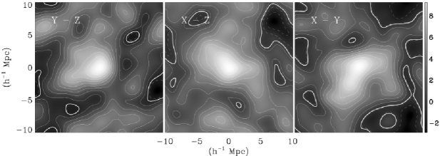
Figure 1.— Initial density field for one of the CR models. Each panel depicts a perpendicular cut of a density cut along the central slice. Continuous lines represent overdensity regions, dashed lines — underdense regions, while the thick line is the mean overdensity within the box. The main constraint of $10^{12}h^{-1}M_{\odot}$ can be noticed at the center of each cut surrounded by the typical large scale structure of the Universe. The gray-scale vertical bar provides the linear density scale.

Figure 1 shows the typical outcome of the CR procedure for one of the models. Each panel shows a 2-D cut (perpendicular to each other) along the central slice of the density field convolved with a Gaussian filter of $10^{12}~{}h^{-1}M_{\odot}$. The continuous lines represent overdense regions, the dashed lines — the underdense ones, while the thick continuous line is the average density within the box. The main constraint can be clearly noticed as the central peak in each panel. It is noteworthy to realize the presence of other smaller peaks surrounding the constrained region. These peaks, which are due to the random component of the CR method, could plausibly lead to major mergers at later epochs with the central overdensity. Smooth accretion of the surrounding matter, together with mergers, make the halos grow continuously, by $z=3$ they have a mass $\sim 10^{13}M_{\odot}$ (see Sec 3.2). Such halos, together with their surrounding environment could potentially be the protocluster regions (e.g., Venemans et~al., 2007) (see also Figure 3).

The UCR set was constructed using the same cosmological parameters, grid and box sizes and random seeds, without imposing any constraint within the fields, resulting in a truly corresponding unconstrained field of the CR one. Figure 2 depicts the central slice of a CR model (left panel) and its UCR counterpart (right panel) from our set. The normalization and contours for both fields are the same in order to stress similarities and differences between the two models. Clearly absent is the peak at the center. However, the overall filamentary structure and underdense regions remain basically the same in both models.

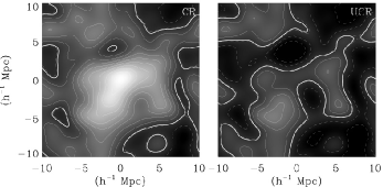
Figure 2.— 2-D cuts of the central slice of thickness $78~{}h^{-1}\mathrm{kpc}$, of the initial density fields for one of our CR models (left panel) and for its respective UCR counterpart (right panel). Despite the main feature missing in the UCR model, the overall LSS is the same in both models. The contour lines are the same for both models.

2.2. Numerical simulations

The $10+10$ simulations were performed with vacuum boundary conditions and physical coordinates. Due to these choices, a sphere of radius $10~{}h^{-1}\mathrm{Mpc}$ was carved out from each of the initial fields and evolved from $z=199$ until $z=3$ by means of the FTM-4.5 code (Heller & Shlosman, 1994; Heller et~al., 2007). The mass resolution within our simulations, under the cosmological model assumed, is of $m=2.95\times 10^{8}M_{\odot}$. Therefore, a galactic mass halo of $10^{11}h^{-1}M_{\odot}$ or above can be resolved with at least 1,000 particles.

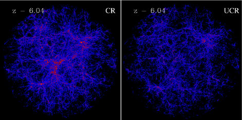
Figure 3.— Typical $N$-bodyoutcome at $z\sim 6$ for a CR model (left panel) and its respective UCR (right panel). These models are the evolved fields of Fig. 2. Colors are proportional to their local densities. The box size is $20$ Mpc for both models.

Figure 3 depicts the typical outcome for two of our simulations, one CR (left panel) and its corresponding UCR realization (right panel) at $z\sim 6$. Both models correspond to the initial conditions maps shown in Fig. 2. Colors in both plots are proportional to their local particle density and they have been equally normalized for a better comparison. The box size in both cases is $20$ Mpc. The most striking feature in the CR frame is the clustering of several halos of similar sizes and masses (see sec.3.1) around the central peak. Such clustering is absent in the UCR. One could naively assume that since there is only one constraint imposed onto the CR model, there should be only one halo of such mass present in the field. However, this is not the case as depicted in Fig. 3, a situation present in all of our models. The presence of other equally massive or slightly smaller structures around the QSO-constrained halo are due to the fact that the imposed constraint excites the formation of structures around it. This provides a higher density environment with respect to a “normal” environment, as shown in the right panel of Fig. 3. Such a behavior is a natural consequence of the hierarchical nature of the underlying CDM model.

2.3. Halos

DM halos were identified by means of the HOP algorithm (Eisenstein & Hut, 1998). This method isolates structures according to a purely density particle criteria. Densities have been calculated locally using an Smooth Particle Hydrodynamics (SPH) kernel. A structure or halo was defined as that region with a 3-D overdensity contour 200 times the mean density. The lower cut in halo mass resolution was at $N=100$ particles or $2.95\times 10^{10}M_{\odot}$ to ensure that the derived halo masses are robust (Trenti et al., 2010). Figure 4 shows (central region of 6 Mpc) the typical outcome for the CR set. The circles are proportional to their virial mass. Notice that apart from the central halo with a mass $>10^{12}M_{\odot}$, there are two other halos of the same mass order. Furthermore, the presence of several $10^{11}$ and in particular of $10^{10}M_{\odot}$ halos is overwhelming. The latter halos follow the distribution of the more massive halos, indicating that the mass growth of such halos will continue substantially. The general excess of halos at any mass scale with respect to a “normal” (unconstrained) field can be easily noticed in their respective mass functions.

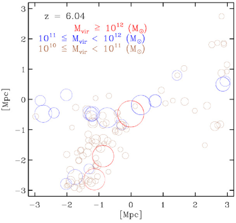
Figure 4.— Halo distribution at $z\sim 6$ for a CR model (same as in previous figures). Circle sizes are proportional to their masses. The box size is 6 Mpc.

3. Results

3.1. Halo mass function

We have constructed halo Mass Functions (MF) from the halo catalogs for each model set, CR and UCR respectively. Figure 5 shows the total MFs averaged for the two sets of 10 realizations, and the comparison Extended Press-Schechter curve (EPS Bond et~al., 1991) in a spherical subvolume of radius $6~{}{\rm Mpc}~{}h^{-1}$ around the QSO halo location for each corresponding QSO – UCR simulation pair in our $10+10set$. Predictions for the mass function of the QSO halos runs have been obtained by taking into account the average linear overdensity inside this sphere introduced by imposing the constraint. The presence of such overdensity changes the effective cosmology (e.g., Goldberg & Vogeley, 2004). The shaded area represents the 68% confidence interval, derived from the $\pm 1\sigma$ variation in the linear overdensity distribution from the set of 10 CR runs. Noteworthy is the effect of the constraints imposed on the field at all mass scales. The MFs show that there is not only a difference at the high mass end range (imposed constraints regime), but the difference persists over the entire mass range. This result is in agreement with the hierarchical nature of the underlying CDM scenario. One would expect a better correspondence between the two MFs in the lower mass end, since the formation of smaller mass halos $(M<10^{10}M_{\odot})$ is more common at these high redshifts. Indeed, such an agreement can be better noticed in Figure 6, where we split the MFs into two regions. The left panel represents the MFs of the inner box of 6 Mpc side centered around the main constraint (in the UCR cases we used the CR counterpart centers). Within this region the differences between both curves should be more striking. Outside this region, the corresponding MFs should have a better agreement as can be noticed on the right panel of Fig. 6. The two MFs differ in less than $5\%$ overall (lower panel), which can be attributed to the fact that the region influence by the constraint is somewhat larger than a radius of 3 Mpc.

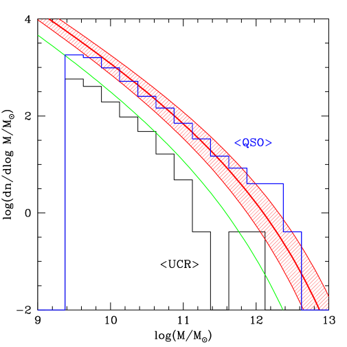
Figure 5.— Average Mass Functions for the two sample sets within a sphere of radius of $6~{}h^{-1}\mathrm{Mpc}$. The continuous lines are the expected number counts derived from the Extended Press-Schechter (EPS, Bond et al. 1991) formalism, for QSOs (red line) and UCRs (green line). The shaded areas represent the 68% confidence interval for a single realization of a CR run as derived from the linear overdensity variance among the sample of CR runs. Effectively, because we are showing a mass function averaged over 10 realizations, the shaded area is more significant.

The corresponding inner MFs show that the environment around a prospective QSO-host halo should be very rich in (sub)structure, at mass levels smaller than $10^{12}M_{\odot}$. A massive halo appears not only to induce the formation of much smaller-scale, $M<10^{10}M_{\odot}$ halos, which one would expect to find here anyway, but also on all intermediate mass-scales which are rare at such redshifts. The relatively high amount of $10^{11}M_{\odot}$ halos ($\sim 10$ on average) exceeds the expectations of those from unconstrained simulations, as shown by the total UCR MF (Figs. 5, 6 right panel).

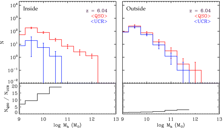
Figure 6.— Average Mass Function for the two sample sets within a box of 6 Mpc (left panel), and outside this inner box (right panel).

Figures 5 and 6 show that the potential QSO fields reside in anomalously dense environments.

3.2. MAH: Fate of the QSO-host halos

The next logical step is to ask what is the fate of such high-density regions? Do they evolve into the most massive clusters nowadays or to a more “normal” cluster-group size halos? Majority of the performed work in this field indeed assumes that high-redshift QSOs can exist only in the precursors of what is now the most massive clusters ($m>10^{15}M_{\odot}$) in the universe (e.g., Springel et~al., 2005; Li et~al., 2007). Such an assumption seems natural since the DM halos can only grow with time.

However, it has been shown that this rule might not necessarily be true, both by means of the EPS formalism and by the analysis of the Millennium simulation (Springel et~al., 2005) merger tree history (De Lucia & Blaizot, 2007; Trenti et~al., 2008; Overzier et~al., 2009). The present DM mass of the QSO-host halos identified at $z\sim 6$ could be of the order of $m\sim 10^{14}M_{\odot}$, and most massive halos identified at various redshifts do not necessarily maintain this property at lower redshifts.

This effect is confirmed in our simulations, although they have been stopped at $z=3$. Throughout their evolution, the halos have experienced a series of major mergers and have grown to $\sim 6\times 10^{12}M_{\odot}$. The most massive halo at $z=3$, the QSO9 has grown to $\sim 10^{13}M_{\odot}$, although it is far from being most massive at $z\sim 6$. We have constructed the Mass Accretion Histories (MAHs) for each of the QSO-host halos in our CRs set. For this purpose, we have reproduced their respective merger trees and followed the branch that represents the constrained halo, at $z=6$, imposed by the initial conditions.

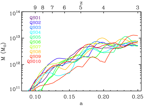
Figure 7.— Mass Accretion Histories (MAHs) for all CR models as a function of redshift $z$ (upper axis) and cosmological expansion factor $a$ (lower axis).

Figure 7 represents the MAHs for all CR models. Most of them (apart from model QSO9) follow the similar trajectories. The abrupt mass increases in the MAH curves are associated with major mergers (e.g., Romano-Díaz et~al., 2006, 2007), which seem to occur at all calculated redshifts. If we compare our MAHs with the cluster sample of Tasitsiomi et~al. (2004) and their fitted MAH, we find that our halos will end up as a normal cluster size halos. Furthermore, a simple estimate accounting for all the mass that could collapse into such DM halos from $z=3$ till the present time, indicates that halos will grow to $\sim 9\times 10^{13}-2\times 10^{14}M_{\odot}$.

The natural dispersion of the MAH curves in Fig. 7 appears to be the result of the cosmic variance and comes from varying the seed of the initial conditions. A striking feature of these curves is their relative evolution. For example, the curve corresponding to QSO10 appears to be least massive of the sample at $z\sim 6$ while it grows fast and becomes the most massive at $z\sim 3$.

4. Comparison with observations: predictions for galaxy counts in QSO fields

QSO Fields	S1	S2	S3
GOODS	$8.08\pm 2.84$	$3.95\pm 1.99$	$2.96\pm 1.72$
J1030$+$0524	+$5.92\pm 4.70$	+$4.05\pm 3.46$	+$7.04\pm 3.60$
J1049$+$4637	-$0.08\pm 4.02$	-$1.95\pm 2.81$	+$1.04\pm 2.64$
J1148$+$5251	-$5.08\pm 4.02$	-$1.95\pm 2.81$	-$2.96\pm 3.60$
J1306$+$0356	-$7.08\pm 4.02$	-$3.95\pm 2.81$	-$1.96\pm 2.43$
J1630$+$4012	+$2.92\pm 4.37$	+$4.05\pm 3.46$	+$2.04\pm 2.82$
Mean	-$3.40\pm 1.89$	+$0.05\pm 1.38$	+$1.04\pm 1.37$

Note. — Number of $i_{\rm 775}$-dropouts and Poisson Error by S/N and Color Limit from Kim et~al. (2009): (1) observed QSO fields; (2) extra-galaxies in the S1 sample (i.e., the GOODS field subtracted from the actual galaxy count in Kim et al. [2009]); (3) extra-galaxies in the S2 sample; (4) extra-galaxies in the S3 sample. Except in the GOODS line, all numbers have GOODS fields subtracted. The S1 – S3 samples are defined in the text. These numbers do not include the target QSO galaxies. The signs “+” mean overdensity and “–” mean underdensity with respect to the GOODS fields (first line). The ‘Mean’ value for S3 refers to mean galaxy counts in 5 observed fields (not to excess counts).

ID	Duty-Cycle	$M_{\rm min}$	UCR	CR (QSO)	Extra-galaxies expected
(Kim et~al.)	$\epsilon_{\rm DC}$	$(10^{10}~{}h^{-1}M_{\odot}$)	Halos	Halos
S3	1.0	11.90	0.15	13.4	13
S2	1.0	11.10	0.2	14.5	14
S1	1.0	8.80	0.6	18.6	18
S3	0.5	10.60	0.3	15.2	7
S2	0.5	8.80	0.4	18.7	9
S1	0.5	6.38	1.2	28.1	13
S3	0.2	6.76	0.7	26.8	5
S2	0.2	5.84	1.0	31.2	6
S1	0.2	4.08	3.0	48.5	9
S3	0.1	4.66	1.5	40.9	4
S2	0.1	4.11	2.0	48.1	5
S1	0.1	2.83	6.1	69.7	6

Note. — Predicted galaxy counts: (1) the samples from Kim et~al. (2009); (2) the duty cycle; (3) minimum DM halo mass — $M_{\rm min}$; (4) the UCR halos; (5) the QSO halos counts which represent the average number of halos in the respective sets more massive than $M_{\rm min}$; (6) the extra number of galaxies expected. All values have been averaged over 10 CRs and 10 UCRs.

Pure DM simulations can be used to predict the expected Lyman Break Galaxies number counts in the Kim et~al. (2009) observations by making additional assumptions. The QSO host galaxy is not counted in the following statistics. First, for simplicity, we assume that one galaxy is found per one DM halo. Second, based on the field of view geometry of the Kim et~al. (2009) observations, we compute the comoving volume probed in an ACS field of view, 11.3 arcmin², i.e., $6\times 6~{}(h^{-1}\mathrm{Mpc})^{2}$ at $z\sim 6$, for $i$-dropouts. Assuming a pencil beam geometry and redshift uncertainty of $\Delta z=1$ centered at $z=6$, we obtain $6\times 6\times 317~{}(h^{-1}\mathrm{Mpc})^{3}$ from the cosmic variance calculator of Trenti & Stiavelli (2008). The effective volume for the search is however smaller due to both incompleteness and because the faint $i$-dropout sources cannot be detected if they are found in the proximity (or behind) brighter foreground galaxies and stars. Based on artificial source recovery simulations carried out to search for $z ≳5$ galaxies (e.g., Oesch et~al., 2007), we estimate that the effective volume is typically one half of the pencil beam volume. Hence, we assume that each ACS field in the Kim et~al. observations has probed $∼5,706~(h^-1 Mpc)^3$.

Two values for S/N color limits of $i_775- z_850=1.3$ and 1.5 have been considered. Choice of S/N $> 5$ and $i_775-z_850 > 1.3$ have been labeled S1; S/N $> 5$ and $i_775-z_850 > 1.5$ have been labeled S2; and S/N $> 8$ and $i_775-z_850 > 1.3$ have been labeled S3.

Table~4 reproduces the observational counts in all QSO fields (Kim et~al., 2009) with one difference --- the GOODS counts have been subtracted. So each number, with the exception of the GOODS field, represents the extra-galaxy counts.

We use the galaxy counts in the GOODS field, as reported in the first data line of Table~4, to derive the number density of $i$-dropouts galaxies in a typical region of the universe at $z ∼6$, depending on the different observation selection procedures in Kim et~al.. These number densities have been compared to number densities of DM halos derived from our sample of unconstrained control simulations.

The minimum DM halo mass, $M_min$, required to match the observed number density of galaxies has been calculated by assuming a given duty cycle $ϵ_DC$ for the Lyman Break Galaxies. The resulting $M_min$ is reported in Table~4 for different values of $ϵ_DC$ and for the different selections S1 -- S3. The values of $M_min$ are consistent with those derived from a conditional luminosity function approach (Stark et~al., 2009; Lee et~al., 2009; Trenti et~al., 2010), as well as from the clustering properties of $i$-dropouts (Overzier et~al., 2006).

Next, we have considered the CR runs and counted the average number of halos with $M ≥M_min$ in the proximity of a QSO host halo, using a pencil beam volume of $6 ×6 ×12~(h^-1 Mpc)^3$ centered at the QSO position. The volume size is determined by the ACS field of view and by the limits imposed by the size of our simulation box. The depth of $12~h^-1 Mpc$ guarantees that the volume considered does not extend outside the simulation computational volume, which is progressively reduced as the overdensity imposed at the center of the box collapses. We have subtracted the number of UCR halos above $M ≥M_min$ (column~4 of Table~4) from that of QSO halos in the pencil beam volume around the QSO (column~5 of Table~4). After multiplying this excess number by $ϵ_DC$, we have obtained the excess number of galaxies predicted in a QSO field compared to the GOODS field (last column in Table~4). For a typical duty cycle values of 0.2 (e.g., Wyithe & Loeb, 2006; Stark et~al., 2007; Lee et~al., 2009; Trenti et~al., 2010), we expect $∼5-9$ more galaxies in the QSO fields, depending on the observational selection criteria, S1 -- S3. We note also that while the above value of $ϵ_DC$ appears as a peak in the likelihood countours, it is a very shallow maximum (e.g., Stark et~al., 2007). A variation in $ϵ_DC$ value between 0.1 and 0.5 does not substantially change the result of the galaxy counts within each of the samples, S1 -- S3.

The galaxy counts in Table~4 do differ when various samples are compared. If we restrict ourselves to the conservative S3 sample, because it has the highest S/N value, the predicted overdensity corresponds to $∼5$ extra galaxies, averaged over 10 QSO fields.

Comparison between the observational counts in Table~4 and predictions from numerical simulations in Table~4 shows that a broad disagreement exists between both counts of extra galaxies. Observational counts in each sample are consistent with no galaxy overdensity or underdensity in the QSO fields, except perhaps for QSO J1030 field (overdensity) and J1148 (underdensity). If we put more weight on S3, because it has the highest S/N value, this conclusion strengthtens even more. The average value of galaxy counts in QSO fields in excess of the GOODS fields for the S3 selection is $1.04±1.37$ which is much smaller than the predicted 5 galaxies. This clearly suggests that galaxy formation around a QSO halo does not follow the predictions based on the abundance of DM halos in this environment compared to the field. This discrepancy is further discussed in section~5. A similar conclusion has been also reached by Overzier et al. (2009) based on the counts of simulated dropout galaxies.

Finally, we note that model halos around the QSO are distributed asymmetrically due to the presence of filaments converging at the QSO location (see Figure~4), hence the asymmetry of sources observed in Fig.~6 of Kim et~al. is a natural consequence of the topology of DM halo distribution around the QSO halo.

5. Discussion

Observations by Kim et~al. (2009) appear broadly consistent with there being no overdensity or underdensity in the galaxy counts of QSO fields with respect to the GOODS fields. This result is puzzling in view of the substantial overdensity of DM halos in the vicinity of the QSO host halo in the numerical simulations presented here. Taken at face value, the observations by Kim et al. imply that, at a given mass, DM halos in the vicinity of a bright QSO host less luminous galaxies than DM halos with the same mass in the control GOODS fields.

On the other hand, Kim et~al. find that the $i_775-z_850$ color distribution of dropout galaxies differs significantly from the averages for the GOODS galaxies similarly selected, at 99% confidence level. This suggest that despite having a comparable average number of galaxies, the QSO fields have observable differences compared to the GOODS fields.

The simplest resolution of this discrepancy may lie in the relatively low number statistics of the Kim et~al. (2009) observations. Only five QSO fields were observed and the number of galaxies detected per field is low (3-8 on average depending on the selection adopted). In fact, if the galaxy number counts for the QSO fields with S3 selection were drawn from a Poisson distribution with $<N>=8$ (3 galaxies from GOODS plus predicted excess of 5 galaxies), then there is a probability $p ∼0.04$ of measuring on average 4 galaxies per QSO field over the five fields observed. Cosmic variance is likely to increase the field to field variations, increasing $p$. But on the other hand, if the QSO halo is more massive than $10^12 M_☉$ (as for example suggested by Springel et~al. 2005), $∼10^13 M_☉$ (e.g., Dijkstra et al. 2008), the excess number of galaxies in its surroundings will also be higher (see also Munoz & Loeb 2008).

Of course, if the QSO halo is less massive instead, then the Kim et~al. results are instead more likely. As we stated in the Introduction, a number of arguments do point to QSOs residing in the less massive halos (e.g., Walter at al. 2004; Willott et al. 2005; Overzier et al. 2009). We note, that although the duty cycles of AGN, in general, and QSOs, in particular, are hotly debated issues at present, the longest duty cycle among AGN appears to be $∼10^8$~yrs --- that of radio galaxies. This hints at the high-$z$ QSO duty cycle being less than unity.

It is possible that the projected (on the sky) overdensities around the high-$z$ QSOs are not associated with the actual 3-D overdensities, and are the result of contamination by the `field' dropout galaxies (e.g., Overzier et al. [2009]). In their Fig.~15, Overzier et al. exhibit $∼30$ projected overdensities from the Mock Survey of $∼70,000$~arc~min$^2$ area based on the Millennium simulation. Many of these overdensities do not correspond to the 3-D overdensities. Therefore, we estimate the probability of such contamination in the Kim et al. (2009) fields. Kim et al. used the ACS fields which correspond to 1/30 of a 316~arc~min$^2$ GOODS field. Hence, each Kim et al. field is $∼316×30 = 9,480$ times smaller than the Overzier et al. field. Assuming here the worst case scenario that all of the 30 overdense regions in their Fig.~15 are `fake' projection cases, we obtain the probability of such a fake overdensity in Kim et al. field as $30:9,480 = 0.0045$. For 5 fields considered by Kim et al., the combined probability for such a fake overdensity not to be associated with a QSO is $∼0.022$, and hence can be fully neglected by us. Of course they are substantial over a much larger area considered by Overzier et al.

Alternatively to the low number statistics case, we should take into account that Kim et al. found one $2σ$-$3σ$ overdensity, one --- a $2σ$ underdensity field, and three additional ones, with no difference to the GOODS fields (using highest S/N column in Table~1). If taken at face value (that is neglecting likely small number statistics), their observational results are consistent with DM halo clustering (i.e., high density regions) and an overpopulation of galaxies, on one hand, and with the scenario in which additional effects (i.e., ionization or hydrodynamics) could play a more dominant role. Accepting results of pure DM simulations which show a clear overdensity of halos in the QSO field, the problem can lie with our understanding of various feedback mechanisms based on evolution of starbursts and the central SBHs, i.e., in the plausible competition between the positive and negative feedbacks which follow from a number of physical processes. This conclusion is weakened by the apparent coincidence between the three QSO fields and the GOODS fields (Table~4).

The fact that some of the observed QSOs are located in average density regions does not necessary imply that they are also average DM density regions. For example, they could be surrounded by baryon-poor DM halos. A variety of negative feedbacks can contribute in removing baryons from DM halos or halting the star formation at those redshifts, such as the UV background radiation and re-ionization (depending on when it occurred), tidal and ram-pressure (ablation) stripping, and dynamical friction could play a role. On the other hand, highly and poorly collimated outflows from QSOs can provide a positive feedback and even trigger the star formation. The inclusion of baryons in DM simulations can affect the properties of DM structures (e.g., Romano-Díaz et~al., 2009, 2010; Duffy et~al., 2010). High resolution numerical simulations will be necessary to investigate these and other effects.

Do the Kim et~al. density estimates reflect the actual local densities or ``projected'' density enhancements along the pencil surveys? Observational evidence from other QSOs at lower redshifts seems to confirm the Kim et al. conclusions --- the QSOs reside in different environments (Stevens et~al., 2010). In fact, Kim et al. reports a confidence estimate at the $95%$ level. Maselli et~al. (2009), using a different method than Kim et al., have arrived at similar conclusions. Of course, it is not straightforward to relate the mass accumulation and environment evolution of high-$z$ QSOs with those at low redshifts.

In a recent development, Utsumi et al. (2010) have used the large field of view of the Suprime-Cam to image of the most distant QSO J2329-0301 at $z=6.42$ and an empty field for comparison. This field of view is about two orders of magnitude larger than the HST/ACS field of view we have considered here (approximately $0.25~deg^2$ versus approximately $11~arcmin^2$). Seven LBG candidates have been found in the QSO field compared to only one LBG in the comparison field. The authors point out that the statistical significance of this apparent overdensity is difficult to estimate. Some evidence exists that the LBGs near the QSO avoid the 3~Mpc region centered on the QSO --- if confirmed this hints to a substantial feedback from the QSO. Extension of this study to additional $z∼6$ QSOs would be very useful to confirm widespread presence of the galaxy overdensity over large scale. After all, the first report on the HST/ACS imaging campaign of $z∼6$ QSOs showed a clear overdensity of LBGs for the single field analyzed (Stiavelli et al. 2005).

We now return to the more pessimistic conclusion from our comparison between the observational galaxy counts and their numerical predictions from our simulations. Can this discrepancy be bridged if one assumes bias between the DM and baryon distribution? Our assumption that there is only one galaxy per DM halo could indeed be an oversimplification. However, an increase in the number of galaxies per host halo will only aggravate the problem, as this will increase the numerical counts.

An interesting by-product of our analysis of the MAH curves for the QSO halos is the observation that the most massive halos at high redshifts do not necessarily remain the most massive ones at lower redshifts, as exhibited by Fig.~7 (see also De Lucia et al 2007; Trenti et al. 2008; Overzier et al. 2009). There are corollaries when looking for possible low-$z$ counterparts of high-$z$ objects. There are a number of issues related to this problem. First, will the SBH grow in tandem with its host DM halo? If yes, we expect SBH masses of the order of a few$×10^10~M_⊙$ in the contemporary universe. Using the comoving volume density of high-$z$ QSOs we estimate at least one such ultra-massive SBH within a sphere of $z$<$$\sim$0.2$. There are no observational constraints at present to rule out such possibility.

However, the situation is aggravated because the most massive halos today have not been most massive at $z∼6$, as our simulations show (see also Trenti et~al. 2008 for an analysis of the Millennium simulation merger tree history and EPS modeling). In turn, this implies that in the local universe there are SBHs more massive than the descendants of the $z ∼6$ QSOs, if the SBH mass is correlated with the DM halo mass (El-Zant et~al., 2003; Ferrarese & Ford, 2005). That may be contradicted by observations as such massive objects will profoundly change the galactic dynamics because the radius of influence of a few$×10^10~M_⊙$ SBHs will be of the order of the visible galaxy.

6. Conclusions

We have performed a set of carefully designed DM $N$-body simulations aimed at studying the environment of QSO-host halos at $z∼6$. A set of 10 Constrained Realizations has been constructed, seeding them with a $10^12M_⊙$ DM halo designed to collapse by $z∼6$ in the top-hat scenario. As a control sample, we performed a set of 10 simulations that represent the Unconstrained Realizations of the same CR set. We have constructed the halo Mass Functions from each simulation and showed how on average, the QSO (i.e., constrained) sample enhanced the DM halo formation in its vicinity due to pure gravitational effects, when compared with its respective UCR sample. Assuming that there is no bias in baryon distribution with respect to the DM in our simulations and that the QSO duty cycle is unity, we have calculated the expected Lyman Break Galaxies number counts and compared this against the observed QSO fields of Kim et~al. (2009).

Our main result is that the pure DM numerical simulations predict a strong overdensity around the QSO peaks. The observations of Kim et~al. (2009) either do not support this or provide a mixed result with one possibly overdense field, one weakly underdense, and three having the density of the GOODS field. The explanation for this discrepancy can lie in the small number of QSO fields observed coupled with the small number of galaxies detected per field. To rule out such possibility it would be important to extend the Kim et al. study to a larger number of $z ∼6$ QSO fields.

If, however, the over/underdensity result will be confirmed by higher S/N observations, the resolution is probably related to the complex physics of feedback mechanism involving the QSO and possibly the starbursts in the surrounding galaxies, or both. With the present analysis we are not capable (nor it was our intention) to establish the role of feedback in the QSO-host galaxy formation evolution. However, our results suggest that in the case of high density QSO environments, the absence of a comparable enhancement of galaxy counts or their lack would point to a strong radiative and/or mechanical negative feedback from the QSOs, resulting in a strong biasing between the DM and baryon distribution.

A simple analysis of the halo-growth in our CR sample together with their MAHs, indicates that these halos will possess, by $z=0$, a mass in the range of $∼10^14 M_⊙$. This is consistent with our choice of a perturbation mass at the initial conditions.

The underdense field J1148 of Kim et~al. that is especially at odds with our numerical expectations, opens the possibility to future investigations adding baryons to simulations to explore the roles of feedback in the evolution of QSO environment, star formation, among other relevant physical phenomena.

But perhaps, not all high-$z$ QSOs are formed in high density peaks but in less massive (and more common) halos of $∼10^11~M_⊙$. The MAHs of our models show that there is natural dispersion (cosmic variance) for the halo masses at each $z$ --- halos which are most massive at $z∼6$ in fact appear least massive at $z∼3$. Hence, QSOs could be surrounded by a more ``typical'' environment, like in the case of J1048+4637 of the Kim et~al. sample (see a similar conclusion by De Lucia & Blaizot (2007) and Overzier et al. [2009]). If this is the case, a scenario in which negative feedback dominates might not be the only solution. Alternatively, $z∼6$ QSOs residing in lower mass halos will require evolution of the $M_∙-σ$ correlation with $z$.

Appendix A Constrained Realizations: New Formalism

One of the key ingredients of the canonical model is that the primordial perturbation field constitutes a random Gaussian field. Hence the setting of initial conditions (ICs) for cosmological simulations amounts to sampling such fields. Gaussian random fields are uniquely determined by their power spectrum, and the assumed statistical homogeneity of the universe, and hence of the perturbation field, implies that Fourier modes of the field are uncorrelated. It follows that an unconstrained realization a of Gaussian field can be performed by sampling the independent Fourier modes from a normal distribution. Here an unconstrained realization of a Gaussian filed means that the realization obeys no other constraint but the assumed power spectrum.

A constrained realization (CR) of a Gaussian field is a random realization of such a field constructed to obey a set of linear constraints imposed on the field. The imposed constraints violates the statistical homogeneity of the field, hence the random sampling of the Fourier modes cannot be used to construct CRs. The Hoffman & Ribak (1991, hereafter HR) provided the optimal algorithm for the construction of CRs and it used here for setting the ICs (see Zaroubi et~al., 1995; Hoffman, 2009).

The aim is to construct random realizations of a Gaussian field, defined by the WMAP5 power spectrum, constrained to have a local density maximum on a mass scale $M_s$ centered at the center of the computational box and designed to collapse by a redshift $z_coll$. The linear overdensity corresponding to the assumed redshift of collapse is calculated by the non-linear top-hat model (e.g., Łokas et~al., 2004, and refs. therein). The field under consideration is the linear fractional overdensity, $δ(r)$, and the constraints corresponds to the $δ$ field smoothed with a kernel corresponding to $M_s$, $Δ_s(r)$. A local density maximum is defined by 10 constraints: the value of $Δ_s$, the three components of its gradient and the 6 independent components of the Hessian of the field. The three first derivatives are set to zero, and the second derivatives are set according the theory of the Gaussian statistics of local density maxima (Bardeen et~al., 1986). This can be fully integrated into the HR algorithm, but it introduces a considerable computational complexity (van de Weygaert & Bertschinger, 1996). Alternatively the local maximum can be constructed by constraining the value of $Δ_s$ at the location of the peak and on six points located along three orthogonal directions, at distances of the order of the smoothing length corresponding to $M_s$. Given the three angles defining the three orthogonal axes these constitute 10 constraints. The off-peak values can be calculated by using the full Gaussian statistics machinery of Bardeen et~al. (1986).

Before the proceeding to the construction of CRs the smoothing kernel needs to be specified. Analytic considerations favor the use of a top-hat filter. However, the sharp real space cut-off leads to the Gibbs Phenomenon, the so-called in k-space, namely the 'ringing' of corresponding fields in k-space. To avoid that a Gaussian filter is adopted here. Namely,

$$\Delta_{\rm s}({\bf r})={1\over(2\pi R{^2_{\rm s}})^{3/2}}\int\exp\biggl{(}-{|{\bf r}-{\bf r}^{\prime}|^2\over 2R{_{\rm s}^2}}\biggr{)}\delta({\bf r}^{\prime})\mathrm{d}^3{\bf r}^{\prime}.$$ (A1)

The smoothing length is related to $M_s$ by

$$R_s=0.64\biggl{(}{3M_{\rm s}\over 4\pi\bar{\rho}}\biggr{)}^{1/3},$$ (A2)

where $ ¯ρ$ is the mean cosmological density (Bardeen et~al., 1986).

Given a random realization $~δ(r)$ and a set of constraints ${Δ_s(r_α)_α=1, ..., 7}$, where $r_α$ is the location at which the $α$ constraint is imposed, a CR is obtained by:

$$\delta^{\rm CR}({\bf r})=\tilde{\delta}({\bf r})+\xi_{\delta,\Delta_{\rm s}}({\bf r}-{\bf r}_\alpha)\Big{(}\xi_{\Delta_{\rm s},\Delta_{\rm s}}({\bf r}_\alpha{\bf r}_\beta)+\sigma{^2_\alpha}\delta{^K_{\alpha,\beta}}\Big{)}^{-1}\Big{(}\Delta_{\rm s}({\bf r}_\beta)-\tilde{\Delta}_{\rm s}({\bf r}_\beta)\Big{)},$$ (A3)

where $P(k)$ is the power spectrum. The various terms that appear in Eq.A3 are defined as follows. The cross-correlation function of the underlying and the smoothed $δ$ fields is given by:

$$\xi_{\delta,\Delta_{\rm s}}=\sqrt{2\over\pi}\int\exp\biggl{(}-{k^2R{_{\rm s}^2}\over 2}\biggr{)}P(k)k^2\mathrm{d}k.$$ (A4)

The auto-correlation function of the smoothed field is given by:

$$\xi_{\Delta_{\rm s},\Delta_{\rm s}}=\sqrt{2\over\pi}\int\exp\big{(}-k^2R{_s^2}\big{)}P(k)k^2\mathrm{d}k$$ (A5)

The pseudo constraints $~Δ_s(r_β)$ are obtained by convolving the random $~δ(r)$ with the Gaussian filter, evaluated at the position of the constraints. The $σ^2_αδ^K_α,β$ term in the inverse of the auto-correlation matrix adds the possibility of a $σ_α$ 'fuzziness', or uncertainty, in the value of the imposed constraint $Δ_s(r_α)$. ($δ^K_α,β$ is the Kronecker $δ$.)

The mean density field around a given density maximum is determined by the assumed power spectrum, the height of the maximum and the Hessian matrix (Bardeen et~al., 1986). It can be shown that for high peaks the mean density profile around the peak is closely approximated by the mean field around a random field point. This property is used here to calculate the values of the off-peak constraints. The mean field around a filed point, constrained to obey just $Δ_s(r=0)$, is given by the Wiener Filter estimator (Zaroubi et~al., 1995; Hoffman, 2009), which is easily obtained from Eq.~A3 by setting $~δ(r)$ to zero. It follows that the construction of a CR proceeds in two steps. First, a single constraint is imposed and the mean field given the constraint is constructed. The values of the off-peak constraints are extracted from the mean field. Then, having the full set of constraints at hand the ensemble of CRs is constructed.

The present implementation of the CR algorithm improves on the earlier utilization of the method employed by Romano-Díaz et~al. (2006, 2007, 2008). There DM halos were imposed by using one single constraint for a given halo, i.e. halos have been treated as random field points as far as the constraints are considered. The present implementation results in better constrained halos, which faithfully obey the imposed (linear) constraints. In particular the virial mass of the imposed halo is very close to the imposed $M_s$ and it is situated very close to the position imposed by the constraints.

# & X [Mpc~$h^-1$] & Y [Mpc~$h^-1$] & Z [Mpc~$h^-1$] & $Δ_s$ & $σ$
1 & 0.0 & 0.0 & 0.0 & 9.05 & 0.0
2 & -0.94 & 0.0 & 0.0 & 8.39 & 0.1
3 & 0.94 & 0.0 & 0.0 & 8.39 & 0.1
4 & 0.0 & -0.94 & 0.0 & 8.39 & 0.1
5 & 0.0 & 0.94 & 0.0 & 8.39 & 0.1
6 & 0.0 & 0.0 & -0.94 & 8.39 & 0.1
7 & 0.0 & 0.0 & 0.94 & 8.39 & 0.1

Table 1 The positions and values of the constraints used to construct the set the initial conditions of the simulations.

The set of constraints used for a mass scale $M_s=10 ^12M_⊙h^-1$, where $h$ is Hubble's constant in units of $100~km~s^-1~Mpc^-1$, collapse redshift of $z_coll=6.0$ and the assumed WMAP5 cosmology is presented in Table~1. For simplicity the realizations are evaluated at the present epoch, $z=0$, and are then scaled down their initial values by the linear growth factor of the WMAP5 cosmology.

References

- Bardeen et~al. (1986) Bardeen, J.~M., Bond, J.~R., Kaiser, N., & Szalay, A.~S. 1986, ApJ, 304, 15
- Barkana (2002) Barkana, R. 2002, New Astronomy, 7, 85
- Barth et~al. (2003) Barth, A.~J., Martini, P., Nelson, C.~H., & Ho, L.~C. 2003, ApJ, 594, L95
- Becker et~al. (2001) Becker, R.~H., et al. 2001, AJ, 122, 2850
- Begelman & Cioffi (1989) Begelman, M.~C. & Cioffi, D.~F. 1989, ApJ, 345, L21
- Bertschinger (1987) Bertschinger, E. 1987, ApJ, 323, L103
- Bond et~al. (1991) Bond, J.~R., Cole, S., Efstathiou, G., & Kaiser, N. 1991, ApJ, 379, 440
- Bunker et~al. (2004) Bunker, A.~J., Stanway, E.~R., Ellis, R.~S., & McMahon, R.~G. 2004, MNRAS, 355, 374
- Cen & McDonald (2002) Cen, R. & McDonald, P. 2002, ApJ, 570, 457
- Davis & Peebles (1983) Davis, M. & Peebles, P.~J.~E. 1983, ApJ, 267, 465
- De Lucia & Blaizot (2007) De Lucia, G. & Blaizot, J. 2007, MNRAS, 375, 2
- Dijkstra et~al. (2008) Dijkstra, M., Haiman, Z., Mesinger, A. & Wyithe, J. 2008, MNRAS, 391, 1961
- Duffy et~al. (2010) Duffy, A.~R., Schaye, J., Kay, S.~T., Dalla Vecchia, C., Battye, R.~A., & Booth, C.~M. 2010, MNRAS, 405, 2161
- Dunkley et~al. (2009) Dunkley, J., et al. 2009, ApJS, 180, 306
- Efstathiou & Rees (1988) Efstathiou, G. & Rees, M.~J. 1988, MNRAS, 230, 5P
- Eisenstein & Hut (1998) Eisenstein, D.~J. & Hut, P. 1998, ApJ, 498, 137
- El-Zant et~al. (2003) El-Zant, A.~A., Shlosman, I., Begelman, M.~C., & Frank, J. 2003, ApJ, 590, 641
- Fan et~al. (2004) Fan, X., et al. 2004, AJ, 128, 515
- Fan et~al. (2003) Fan, X., et al. 2003, AJ, 125, 1649
- Ferrarese & Ford (2005) Ferrarese, L. & Ford, H. 2005, Space Science Reviews, 116, 523
- Ferrarese & Merritt (2000) Ferrarese, L. & Merritt, D. 2000, ApJ, 539, L9
- Gebhardt et~al. (2000) Gebhardt, K., et al. 2000, ApJ, 539, L13
- Giavalisco et~al. (2004) Giavalisco, M., et al. 2004, ApJ, 600, L93
- Gnedin & Ostriker (1997) Gnedin, N.~Y. & Ostriker, J.~P. 1997, ApJ, 486, 581
- Goldberg & Vogeley (2004) Goldberg, D.~M. & Vogeley, M.~S. 2004, ApJ, 605, 1
- Graham et~al. (2001) Graham, A.~W., Erwin, P., Caon, N., & Trujillo, I. 2001, ApJ, 563, L11
- Haiman & Holder (2003) Haiman, Z. & Holder, G.~P. 2003, ApJ, 595, 1
- Heller & Shlosman (1994) Heller, C.~H. & Shlosman, I. 1994, ApJ, 424, 84
- Heller et~al. (2007) Heller, C.~H., Shlosman, I., & Athanassoula, E. 2007, ApJ, 671, 226
- Hoffman (2009) Hoffman, Y. 2009, in Lecture Notes in Physics, Berlin Springer Verlag, Vol. 665, Data Analysis in Cosmology, ed. V.~J.~Martinez, E.~Saar, E.~M.~Gonzales, & M.~J.~Pons-Borderia, 565--+
- Hoffman & Ribak (1991) Hoffman, Y. & Ribak, E. 1991, ApJ, 380, L5
- Kaiser (1984) Kaiser, N. 1984, ApJ, 284, L9
- Kim et~al. (2009) Kim, S., Stiavelli, M., Trenti, M., Pavlovsky, C.~M., Djorgovski, S.~G., Scarlata, C., Stern, D., Mahabal, A., Thompson, D., Dickinson, M., Panagia, N., & Meylan, G. 2009, ApJ, 695, 809
- Lee et~al. (2009) Lee, K., et al. 2009, ApJ, 695, 368
- Li et~al. (2007) Li, Y., et al. 2007, ApJ, 665, 187
- Łokas et~al. (2004) Łokas, E.~L., Bode, P., & Hoffman, Y. 2004, MNRAS, 349, 595
- Madau et~al. (1996) Madau, P., Ferguson, H.~C., Dickinson, M.~E., Giavalisco, M., Steidel, C.~C., & Fruchter, A. 1996, MNRAS, 283, 1388
- Magorrian et~al. (1998) Magorrian, J., et al. 1998, AJ, 115, 2285
- Marconi & Hunt (2003) Marconi, A. & Hunt, L.~K. 2003, ApJ, 589, L21
- Maselli et~al. (2009) Maselli, A., Ferrara, A., & Gallerani, S. 2009, MNRAS, 395, 1925
- Muñoz & Loeb (2008) Muñoz, J.~A. & Loeb, A. 2008, MNRAS, 385, 2175
- Oesch et~al. (2007) Oesch, P.~A., et al. 2007, ApJ, 671, 1212
- Overzier et~al. (2009) Overzier, R.~A., Guo, Q., Kauffmann, G., De Lucia, G., Bouwens, R., & Lemson, G. 2009, MNRAS, 394, 577
- Overzier et~al. (2006) Overzier, R.~A., Bouwens, R.~J., Illingworth, G.~D., & Franx, M. 2006, ApJ, 648, L5
- Rees (1989) Rees, M.~J. 1989, MNRAS, 239, 1P
- Romano-Díaz et~al. (2006) Romano-Díaz, E., Faltenbacher, A., Jones, D., Heller, C., Hoffman, Y., & Shlosman, I. 2006, ApJ, 637, L93
- Romano-Díaz et~al. (2007) Romano-Díaz, E., Hoffman, Y., Heller, C., Faltenbacher, A., Jones, D., & Shlosman, I. 2007, ApJ, 657, 56
- Romano-Díaz et~al. (2009) Romano-Díaz, E., Shlosman, I., Heller, C., & Hoffman, Y. 2009, ApJ, 702, 1250
- Romano-Díaz et~al. (2010) ---. 2010, ApJ, 716, 1095
- Romano-Díaz et~al. (2008) Romano-Díaz, E., Shlosman, I., Hoffman, Y., & Heller, C. 2008, ApJ, 685, L105
- Shapiro & Raga (2001) Shapiro, P.~R. & Raga, A.~C. 2001, in Revista Mexicana de Astronomia y Astrofisica Conference Series, Vol.~10, Revista Mexicana de Astronomia y Astrofisica Conference Series, ed. J.~Cantó & L.~F.~Rodríguez, 109--114
- Shaver et~al. (1996) Shaver, P.~A., Wall, J.~V., Kellermann, K.~I., Jackson, C.~A., & Hawkins, M.~R.~S. 1996, Nature, 384, 439
- Shlosman & Phinney (1989) Shlosman, I. & Phinney, E.~S. 1989, unpublished
- Sijacki et~al. (2009) Sijacki, D., Springel, V., & Haehnelt, M.~G. 2009, MNRAS, 400, 100
- Springel et~al. (2005) Springel, V., et al. 2005, Nature, 435, 629
- Stark et~al. (2009) Stark, D.~P., Ellis, R.~S., Bunker, A., Bundy, K., Targett, T., Benson, A., & Lacy, M. 2009, ApJ, 697, 1493
- Stark et~al. (2007) Stark, D.~P., Loeb, A., & Ellis, R.~S. 2007, ApJ, 668, 627
- Steidel et~al. (2003) Steidel, C.~C., Adelberger, K.~L., Shapley, A.~E., Pettini, M., Dickinson, M., & Giavalisco, M. 2003, ApJ, 592, 728
- Stevens et~al. (2010) Stevens, J.~A., Jarvis, M.~J., Coppin, K.~E.~K., Page, M.~J., Greve, T.~R., Carrera, F.~J., & Ivison, R.~J. 2010, MNRAS, 627
- Stiavelli et~al. (2005) Stiavelli, M., et al. 2005, ApJ, 622, L1
- Tasitsiomi et~al. (2004) Tasitsiomi, A., Kravtsov, A.~V., Gottlöber, S., & Klypin, A.~A. 2004, ApJ, 607, 125
- Trenti et~al. (2008) Trenti, M., Santos, M.~R., & Stiavelli, M. 2008, ApJ, 687, 1
- Trenti & Stiavelli (2007) Trenti, M. & Stiavelli, M. 2007, ApJ, 667, 38
- Trenti & Stiavelli (2008) ---. 2008, ApJ, 676, 767
- Trenti et~al. (2010) Trenti, M., et al. 2010, ApJ, 714, L202
- Trenti et al. (2010) Trenti, M., Smith, B.~D., Hallman, E.~J., Skillman, S.~W., & Shull, J.~M. 2010, ApJ, 711, 1198
- Utsumi et al. (2010) Utsumi, Y., Goto, T., Kashikawa, N., Miyazaki, S., Komiyama, Y., Furusawa, H., & Overzier, R. 2010, ApJ, 721, 1680
- van de Weygaert & Bertschinger (1996) van de Weygaert, R. & Bertschinger, E. 1996, MNRAS, 281, 84
- Venemans et~al. (2003) Venemans, B.~P., Kurk, J.~D., Miley, G.~K., & Röttgering, H.~J.~A. 2003, New Astronomy Reviews, 47, 353
- Venemans et~al. (2007) Venemans, B.~P., et al. 2007, A&A, 461, 823
- Walter et~al. (2004) Walter, F., Carilli, C., Bertoldi, F., Menten, K., Cox, P., Fan, X. & Strauss, M.~A. 2004, ApJ, 615, L17
- Willott et~al. (2005) Willott, C.~J., et al. 2005, in Growing Black Holes: Accretion in a Cosmological Context, ed. A.~Merloni, S.~Nayakshin, & R.~A.~Sunyaev, 102--107
- Willott et~al. (2010) Willott, C.~J., et al. 2010, AJ, 139, 906
- Wyithe & Loeb (2003) Wyithe, J.~S.~B. & Loeb, A. 2003, ApJ, 586, 693
- Wyithe & Loeb (2006) ---. 2006, Nature, 441, 322
- York et~al. (2000) York, D.~G., et al. 2000, AJ, 120, 1579
- Zaroubi et~al. (1995) Zaroubi, S., Hoffman, Y., Fisher, K.~B., & Lahav, O. 1995, ApJ, 449, 446
- Zheng et~al. (2006) Zheng, W., et al. 2006, ApJ, 640, 574