Abstract

We analyze the prospect for observing the intermediate neutral Higgs boson ($h_{2}$) in its decay to two lighter Higgs bosons ($h_{1}$) at the presently operating hadron colliders in the framework of the CP violating MSSM using the PYTHIA event generator. We consider the lepton+ 4-jets+ $E\!\!\!\!/_{T}$ channel from associate $Wh_{2}$ production, with $Wh_{2}\rightarrow Wh_{1}h_{1}\rightarrow\ell\nu_{\ell}b\bar{b}b\bar{b}$. We require two, three or four tagged $b$-jets. We explicitly consider all relevant Standard Model backgrounds, treating $c$-jets separately from light flavor and gluon jets and allowing for mistagging. We find that it is very hard to observe this signature at the Tevatron, even with 20 fb^-1 of data, in the LEP–allowed region of parameter space due to the small signal efficiency, even though the background is manageable. At the LHC, a priori huge SM backgrounds can be suppressed by applying judiciously chosen kinematical selections. After all cuts, we are left with a signal cross section of around 0.5 fb, and a signal to background ratio between 1.2 and 2.9. According to our analysis this Higgs signal should be viable at the LHC in the vicinity of present LEP exclusion once 20 to 50 fb^-1 of data have been accumulated at $\sqrt{s}=14$ TeV.

1 Introduction

The Minimal Supersymmetric Standard Model (MSSM) [1] requires two Higgs doublets, leading to a total of five physical Higgs bosons. At the tree level, these can be classified as two neutral CP–even bosons ($\phi_{1}$ and $\phi_{2}$), one neutral CP–odd boson ($a$) and two charged bosons. In the presence of CP violation, the three neutral Higgs bosons can mix radiatively [2, 3]. The mass eigenstates $h_{1}$, $h_{2}$ and $h_{3}$ with $m_{h_{1}}<m_{h_{2}}<m_{h_{3}}$ can then be obtained from the interaction eigenstates $\phi_{1}$, $\phi_{2}$ and $a$ with the help of the orthogonal matrix $O_{\alpha i}$, $(\phi_{1},\phi_{2},a)^{T}_{\alpha}={O_{\alpha i}}(h_{1},h_{2},h_{3})^{T}_{i}\,,$ which diagonalizes the Higgs boson mass matrix. $O$ depends on various parameters of the SUSY Lagrangian.

Due to this mixing, the Higgs mass eigenstates are no longer CP eigenstates. Moreover, the masses of the Higgs bosons, their couplings to SM and MSSM particles, and their decays are significantly modified [3]. For example, the Higgs boson couplings to pairs of gauge bosons are scaled by $g_{h_{i}VV}$ relative to the SM. These couplings can be expressed as $g_{h_{i}VV}=\cos\beta\,O_{\phi_{1}i}\>+\>\sin\beta\,O_{\phi_{2}i}\,,$ where $\tan\beta$ is the ratio of Higgs vacuum expectation values (VEVs). The magnitude of $g_{h_{2}WW}$ is directly related to the production process studied in this paper.

In the absence of mixing between neutral CP–even and CP–odd states the LEP experiments were able to derive absolute lower bounds of about 90 GeV on the masses of both the lighter CP–even Higgs and the CP–odd boson [4]. However, in the presence of CP violation, the LEP experiment were not able to exclude certain scenarios with very light $h_{1}$. In this “LEP hole” $h_{1}$ is dominantly a CP–odd state with almost vanishing coupling to the $Z$ boson. One then has to search for $Zh_{2}$ or $h_{1}h_{2}$ production. In part of the LEP hole, these cross sections are suppressed by the rather large $h_{2}$ mass. Moreover, $h_{2}\rightarrow h_{1}h_{1}$ decays lead to quite complicated final states, which often yield low efficiencies after cuts. One LEP–allowed region has $m_{h_{1}}\raisebox{-3.69899pt}{~{}\shortstack{$<$ \\ [-0.07cm] $\sim$}}~{}10$ GeV, so that $h_{1}\rightarrow\tau^{+}\tau^{-}$ is dominant; in the other, $m_{h_{1}}\sim 30-50$ GeV so that $h_{1}\rightarrow b\bar{b}$ is dominant. $m_{h_{2}}$ lies between slightly below 90 and slightly above 130 GeV. Scenarios with even lighter $h_{2}$ are excluded by decay–independent searches for $Zh_{2}$ production [4, 5, 6]. If $m_{h_{2}}$ is much above 130 GeV, the CP–odd component of $h_{1}$ becomes subdominant, so that the cross section for $Zh_{1}$ production becomes too large. Finally, the LEP hole occurs for $\tan\beta$ in between 3 and 10 [4, 7].

In this paper we analyze the prospect for observing a signal for the production of neutral Higgs bosons in the second of these LEP allowed regions. Since the $h_{1}WW$ coupling is suppressed along with the $h_{1}ZZ$ coupling, we focus on $Wh_{2}$ production, with $h_{2}\rightarrow h_{1}h_{1}\rightarrow b\bar{b}b\bar{b}$ and $W\rightarrow\ell\nu$, where $\ell$ is an electron or muon. This process has recently been studied in refs.[8, 9], using parton–level analyses, with quite promising results. We instead performed a full hadron–level analysis, including initial and final state showering as well as the underlying event. We will see that these effects significantly reduce the basic kinematical efficiencies of the signal, while allowing the background to populate new regions of phase space. Moreover, we have expanded the list of background processes; some of the backgrounds not considered in [9] turn out to be sizable. Altogether this leads to a reduced significance to isolate the signal from the SM backgrounds.

The Higgs boson masses, their coupling to gauge bosons and their branching ratios are also modified in some other models. Examples are scenarios with spontaneous CP violation [10] and models with additional Higgs singlet [11]. The simplest of these is the next–to–minimal supersymmetric standard model (NMSSM) [12], the CP violating version of which has also recently been discussed [13]. In all these scenarios the process we are considering is possible, and might be useful as a discovery channel. For example, in the CP–conserving NMSSM, the role of $h_{2}$ could be played by either the lightest or the second lightest CP–even scalar. In the former case, the role of $h_{1}$ would be played by the lighter CP–odd scalar, whereas in the latter case, the role of $h_{1}$ could also be played by the lightest CP–even scalar [14].

In order to be as model–independent as possible, we chose several benchmark points where we simply fix the masses $m_{h_{1}}$ and $m_{h_{2}}$ as well as the relevant product of couplings and branching fractions. In addition we investigate a couple of benchmark points within the so–called CPX scenario of the MSSM [15], where the masses and couplings of the Higgs bosons can be computed in terms of the fundamental input parameters. We find that the signal can be detectable at the LHC once 20 to 50 fb^-1 of data have been accumulated at $\sqrt{s}=14$ TeV; since in any case a large integrated luminosity is needed, we do not consider scenarios with smaller $\sqrt{s}$. The situation at the Tevatron seems hopeless due to the very small signal.

The remainder of this paper is organized as follows. In Sec. 2 we introduce our benchmark points, and the the numerical procedures to estimate signal and backgrounds. In Sec. 3 results for the Tevatron will be discussed. In particular, we mention the detector parameters, and introduce different (combinations of) kinematical cuts, in order to get rid of the a priori huge SM background and retain as many signal events as possible. Sec. 4 presents a similar analysis for the LHC. Finally we will summarize in Sec. 5.

2 Numerical analysis

In this section we first describe our benchmark scenarios. We then give a list of the background processes we included in our analysis, and discuss the event generation.

2.1 Benchmark scenarios for the signal

In our analysis we took five different benchmark points, denoted by S1 through S5, with different intermediate Higgs boson masses ($m_{h_{2}}$) in between 90 and 130 GeV, while the lighter Higgs boson mass ($m_{h_{1}}$) is fixed at 30 GeV; this resembles the model–independent approach taken in ref.[9]. Note that a Higgs boson with SM–like coupling to the $Z$ (which is equivalent to demanding an SM–like coupling to the $W$) is excluded if its mass is below 82 GeV, independent of its decay mode [5, 6]. On the other hand, in the CP–violating MSSM values $m_{h_{2}}$ significantly above 130 GeV are incompatible with a strongly reduced $ZZh_{1}$ coupling [4]. Moreover, for $m_{h_{2}}>130$ GeV, the standard decays into $WW^{*},ZZ^{*}$ are expected to become dominant, reducing the branching ratio for the $h_{2}\rightarrow h_{1}h_{1}$ decays we are interested in.

In addition we considered two benchmark points in the CPX–scenario of the MSSM [15], which is defined by the following set of input parameters:

$$\widetilde{M}_{Q} = \widetilde{M}_{t}=\widetilde{M}_{b}=500\ {\rm GeV},\qquad\mu=4\widetilde{M}_{Q}\,,$$

$$|A_{t}| = |A_{b}|=2\widetilde{M}_{Q},\qquad{\rm arg}(A_{t})={\rm arg}(A_{b})=90^{\circ}\,,$$

$$|m_{\tilde{g}}| = 1~{}{\rm TeV}\,,\qquad{\rm arg}(m_{\tilde{g}})\ =\ 90^{\circ}\,.$$ (1)

Here $\widetilde{M}_{Q}$ is the mass of third generation $SU(2)$ doublet squarks, and $\widetilde{M}_{t},\,\widetilde{M}_{b}$ are the masses of the corresponding singlets. $\mu$ is the supersymmetric higgsino mass parameter, $A_{b,t}$ are trilinear soft breaking parameters in the sbottom and stop sectors, respectively, and $m_{\tilde{g}}$ is the gluino mass. We work in the convention where $\mu$ is real; in the CPX scenario, $A_{b,t}$ and $m_{\tilde{g}}$ are purely imaginary. The remaining two input parameters are the charged Higgs boson mass $m_{H^{\pm}}$ and $\tan\beta$. We take $M_{H^{+}}=131.8$ GeV, and $\tan\beta=4.02\ (4.39)$ in benchmark point CPX–1 (CPX–2). We calculated the spectrum and the couplings for these two benchmark points using CPsuperH [3]. Other packages like FeynHiggs  [16] can also be used for this purpose. In CPX–1 $m_{h_{1}}$ and $m_{h_{2}}$ are 36 and 101.6 GeV, while in CPX–2, which is close to the upper edge of the LEP allowed region, these masses are 45 and 102.6 GeV respectively.

	mass [GeV]		$\sigma$ [pb]
Scenario	$h_{2}$	$h_{1}$	Tevatron	LHC
S1	130	30	0.090	1.091
S2	120	30	0.122	1.402
S3	110	30	0.163	1.851
S4	100	30	0.223	2.472
S5	90	30	0.315	3.317
CPX–1	102	36	0.212	2.367
CPX–2	103	45	0.206	2.284

Table 1: The seven benchmark scenarios we consider. Scenarios S1 through S5 are defined purely phenomenologically, in terms of the masses of the relevant Higgs bosons, whereas scenarios CPX–1 and CPX–2 have been obtained within the CPX set of the MSSM. The last two columns give the total cross sections for $Wh_{2}$ production at the Tevatron ($p\bar{p}$ collisions at $\sqrt{s}=1.96$ TeV) and the LHC ($pp$ collisions at $\sqrt{s}=14$ TeV), assuming SM–strength for the $h_{2}WW$ coupling.

The seven benchmark scenarios are summarized in Table 1. All of them satisfy $m_{h_{2}}>2m_{h_{1}}$ and $m_{h_{1}}>2m_{b}$, so that the $\ell$+4$j$+$E\!\!\!\!/_{T}$ signal topology that we are interested in can arise from the associated $Wh_{2}$ production at hadron colliders. Note finally that a scenario very similar to S4 can be realized in the CPX framework of the MSSM, with $m_{H^{+}}=127.9$ GeV and $\tan\beta=4.31$.

The last two columns in Table 1 give the total cross sections for $Wh_{2}$ production at the Tevatron ($p\bar{p}$ collisions at $\sqrt{s}=1.96$ TeV) and the LHC ($pp$ collisions at $\sqrt{s}=14$ TeV), assuming SM–strength for the $h_{2}WW$ coupling. We set the factorization scale to $Q=\sqrt{\hat{s}}$ (the partonic center–of–mass energy) and used CTEQ5L [17] for the parton distribution functions (PDF). The production cross section is independent of $m_{h_{1}}$. We see that going from the Tevatron to the LHC increases the cross section by about a factor of eleven.

If the Higgs sector only contains $SU(2)$ doublets and singlets, the $h_{2}WW$ coupling can only be reduced from its SM value by mixing. Moreover, for our signal we require the $W$ boson to decay leptonically, and $h_{2}$ to decay into four $b$ (anti–)quarks via two on–shell $h_{1}$ bosons, thus leading to $\ell jjjjE\!\!\!\!/_{T}$ events, where $\ell=e$ or $\mu$. The cross section for this signal topology can be expressed as

$$\sigma_{\rm signal}^{\rm tot}=\sigma_{SM}(p\bar{p}/pp\rightarrow Wh_{2})\times C_{h_{2}WW}\times 2{Br(W\rightarrow e\nu_{e})}\,$$ (2)

where we have introduced the quantity

$$C_{h_{2}WW}=g^{2}_{h_{2}WW}\times Br(h_{2}\rightarrow h_{1}h_{1})\times Br(h_{1}\rightarrow b\bar{b})^{2}\,.$$ (3)

Here $g_{h_{2}WW}$ is the $h_{2}WW$ coupling in units of the corresponding SM value, and the factor 2 is for $\rm\ell=e$ and $\mu$. We have taken $Br(W\rightarrow e\nu_{e})=0.106$. Following ref.[9], we set $C_{h_{2}WW}=0.50$ in our numerical analysis. This is slightly larger than the values computed for scenarios CPX–1 and CPX–2, which are 0.465 and 0.435, respectively. Our results can trivially be scaled downward by the corresponding factors; however, this correction is smaller than the theoretical uncertainty of our leading order calculation.

2.2 Background processes

We just saw that our signal consists of four jets, one charged lepton, and missing $E_{T}$, where the latter two components come from the decay of an on–shell $W^{\pm}$ boson. In our background estimate we only include processes that lead to the same topology, i.e. we insist on the presence of at least one leptonically decaying real $W^{\pm}$ boson in the event. We thus ignore background contributions where a jet is misidentified as a lepton, as well as backgrounds where the entire missing $E_{T}$ is due to mismeasurements or incomplete coverage of the detector. We trust that these instrumental backgrounds are small after cuts.

However, we do not insist on having four $b$ (anti–)quarks in the event. In fact, we will see shortly that requiring all four $b$ jets in the signal to be tagged as such leads to a very low efficiency, i.e. low signal rate. Moreover, there is a finite probability that jets are mistagged, i.e. are tagged as $b-$jets even though they do not contain a $b-$flavored hadron. We thus include all leading order processes that produce final states containing at least one (leptonically decaying) $W^{\pm}$ boson and at least four jets. This includes $t\bar{t}$ production, as well as processes where the $W^{\pm}$ boson is produced directly rather than from the decay of a top quark.

This latter class of reactions includes a large number of final states. The largest cross sections are for final states not containing any heavy quarks. However, these will be suppressed heavily by $b-$tagging requirements. Processes containing at least a couple of heavy quarks in the final state have smaller cross sections, but much higher efficiencies. In order to obtain a reliable background estimate without having to generate huge numbers of events, we separate the direct $W+4j$ production processes into many categories, according to the number of heavy quarks, light quarks and gluons in the final state. For reasons that will become clear shortly, we also include $t\bar{t}b\bar{b}$ and $t\bar{t}c\bar{c}$ in our background estimate. In the signal, and in all $W+4j$ backgrounds, we force the $W$ boson to decay leptonically. Similarly, in all backgrounds containing a $t\bar{t}$ pair, we force one $W$ boson to decay leptonically, and the second $W$ boson to decay into a tau–lepton or hadronically.

A complete list of the backgrounds we consider is given in Table 2. Processes p2 through p8 are all mixed QCD–electroweak $W+4j$ processes, but differ in the number of $b-$quarks. Process p8, which does not have any $b-$quarks in the final state, has by far the largest cross section. It can be broken up into processes p8.1 through p8.9, which have different numbers of gluons and charm (anti–)quarks in the final state; the latter are treated separately, since charm jets have a much higher probability to be mistagged as $b-$jets than jets originating from light flavors or gluons. Process p8.2, which has the largest cross sections of all, is further broken up according to the charge of the produced $W$ boson.

			$\sigma$ [pb]
label	final state	$j$	Tevatron	LHC
p1	$t\bar{t}$		5.00	500.0
p2	$b\bar{b}b\bar{b}W^{\pm}$		0.015	0.156
p3	$b\bar{b}bjW^{\pm}$	$udscg$	$5\cdot 10^{-5}$	0.011
p4	$b\bar{b}cjW^{-}$	$udsg$	0.152	33.8
p5	$b\bar{b}c\bar{c}W^{\pm}$		0.051	0.521
p6	$b\bar{b}jjW^{\pm}$	$udsg$	5.99	248
p7	$bjjjW^{\pm}$	$udscg$	0.017	3.32
p8	$jjjjW^{\pm}$	$udscg$	447.9	$2.93\cdot 10^{4}$
p8.1	$ggggW^{\pm}$		93.4	918.6
p8.2	$gggjW^{\pm}$	$udsc$	206.4	$1.97\cdot 10^{4}$
p8.2.1	$gggjW^{+}$	$ds$	67.0	9302
p8.2.2	$ggg\bar{j}W^{+}$	$uc$	31.9	1853
p8.2.3	$gggjW^{-}$	$uc$	31.8	5013
p8.2.4	$ggg\bar{j}W^{-}$	$ds$	67.2	1562
$\sum_{i=1}^{4}$ p8.2.$i$			197.9	$1.77\cdot 10^{4}$
p8.3	$ggjjW^{\pm}$	$udsc$	122.6	6476
p8.4	$gjjjW^{\pm}$	$udsc$	25.4	2263
p8.5	$\bar{c}jjjW^{+}$	$uds$	0.435	50.9
p8.6	$c\bar{c}jjW^{\pm}$	$uds$	0.991	33.3
p8.7	$c\bar{c}cjW^{-}$	$uds$	0.094	15.0
p8.8	$c\bar{c}c\bar{c}W^{\pm}$		0.049	0.471
p8.9	$jjjjW^{\pm}$	$uds$	2.67	99.4
$\sum_{i=1}^{9}$ p8.$i$			443.6	$2.76\cdot 10^{4}$
p9	$t\bar{t}b\bar{b}$		0.0090	2.99
p10	$t\bar{t}c\bar{c}$		0.016	4.86
$\sum_{i=1}^{10}$ p$i$			454.9	$2.84\cdot 10^{4}$

Table 2: List of background processes and their total cross sections after the pre–selection cuts (2.2). Charge conjugate final states are included, if they differ from the listed final states, except for processes p.8.2.$i$, $i=1\dots 4$. The symbol $j$ stands for different partons, as listed in the third column, where the corresponding antiquarks are always included. See the text for further explanations.

We used MadGraph/MadEvent v4.4.15 [18] for generating parton level SM $W+4j$ background events and for the calculation of the corresponding cross sections. We simulated $t\bar{t}$ event sample using PYTHIA, assuming $m_{t}=172.6$ GeV as pole mass. We again employ CTEQ5L [17] parton distribution functions, with factorization and renormalization scale given by $\sqrt{\hat{s}}$. We only include $u,d,s$ quarks and gluons in the initial state, since we generate all heavy $c$ and $b$ quarks explicitly; at least in case of $b-$quarks the required transverse momentum is only a few times larger than the mass of the quark, making the use of $b-$quark distributions in the proton questionable. Flavor mixing has been included where appropriate, using current values for the charged current couplings [19].

The resulting cross sections are listed in Table 2. They have been calculated with the following kinematical cuts, also used for the generation of events:

$$p_{T}^{j,b} \geq 5\ {\rm GeV}\,;$$

$$\eta^{j,b} \leq 5.0\,;$$ (4)

$$\Delta R(jj,bb,bj) \geq 0.3\,.$$

Here $\Delta R=\sqrt{(\Delta\eta)^{2}+(\Delta\phi)^{2}}$, where $\eta$ and $\phi$ are the pseudorapidity and azimuthal angle, respectively. Note that some cuts on the partonic transverse momenta, and on the separation between partons, are necessary in order to obtain finite cross sections. We chose pre–selection cuts on the generated partons that are much weaker than our final analysis cuts, since showering can change the transverse momenta and separations significantly.

Note that the sum of subprocess cross sections in Table 2 often does not exactly agree with the total cross section listed first. The reason is that these numbers result from different runs of MadGraph/MadEvent, with the given more or less inclusive final state. Since the total event statistics for the sum of subprocesses is higher, and the cross section calculation becomes more reliable when fewer different subprocesses need to be added, we consider the summed subprocess cross sections more reliable estimates, and use these in the estimate of the total background cross section after pre–selection cuts, which is given in the last line of Table 2.

We see that going from the Tevatron to the LHC increases the raw background cross section for process p2, which most directly resembles our signal, by about the same factor as the signal cross section. However, the cross sections for other background processes increase much more rapidly. This is true in particular for the total $t\bar{t}$ production cross section, process p1, which increases by two orders of magnitude; the cross sections for processes p4 and p6, which increase by factors of 220 and 40, respectively; and for the $t\bar{t}Q\bar{Q}$ cross sections ($Q=b,c$), processes p9 and p10, which increase by a factor of about 300. The smallest ratio obtains for cross sections dominated by $u\bar{d}$ or $\bar{u}d$ annihilation, which includes the signal as well as background processes p2, p5, p8.1 and p8.8. Here the increase is limited by the fact that the LHC is a $pp$ collider, whereas the Tevatron is a $p\bar{p}$ collider. Process p6 receives sizable contributions from $gq$ scattering as well as $gg$ fusion; the corresponding parton fluxes increase faster than the $u\bar{d}$ flux does. Process p4 receives sizable contributions from the $gs$ initial state; contributions with $gd$ initial state are suppressed by a factor $\left|V_{cd}\right|^{2}\simeq 0.053$. Finally, the increase is largest for processes p9 and p10, which at the LHC receive dominant contributions from the $gg$ initial state, but suffer from small parton flux factors at the Tevatron due to the large required partonic center–of–mass energy.

2.3 Monte Carlo simulation

As noted above, all parton–level events have been generated by MadGraph/MadEvent. They are then passed on to PYTHIA v.6.408 [20], which handles initial and final state showering and hadronization; PYTHIA also adds an “underlying event” due to the spectator partons and their interactions. We utilize the “old” shower algorithm based on virtuality ordering. We use the default, large squared shower scale $4\hat{s}$ for the signal as well as for inclusive $t\bar{t}$ production. All other background processes typically include relatively soft particles already at the hadron level; we therefore use a much smaller squared shower scale $\sim 0.002\hat{s}$ for all other background processes. Initial state radiation adds extra energy, and perhaps additional jets, to the event. It can also give it a transverse kick, allowing partons with relatively low transverse momentum in the partonic center–of–mass system to produce jets that pass our acceptance cuts (which are specified below). For our purposes final state radiation is also very important, since it smears out invariant mass distributions, thereby e.g. allowing the reconstructed jets from top decay to have a total invariant mass well below the top mass. We will see below that parton showering, which is not included in earlier parton–level analyses [8, 9], re–establishes $t\bar{t}$ production as most important background after cuts. Note that showering, and hence the choice of showering scale, is much less important for the other background processes.

In roughly 1 to 4% (5 to 15%) of the events, showering will produce at least one additional $b\bar{b}$ ($c\bar{c}$) pair. In almost all background processes including such events would lead to double counting, since the production of final states with multiple heavy quarks has been treated explicitly in our list of backgrounds. For example, producing another $b\bar{b}$ pair when showering an event of type p1 would lead to an event of the type p9; producing a $c\bar{c}$ pair when showering an event of type p6 would yield an event of type p5; and so on. Vetoing these potentially double counted events is rather important, since they can have a much larger efficiency for passing the multi $b-$tag requirement we impose to reduce backgrounds than events without additional heavy quarks from showering. Since such events are rare, they would also lead to very slow convergence of the MC simulation.

Finally, our simulation also includes experimental resolution smearing for the jet angles and energies, using the toy calorimeter PYCELL provided by PYTHIA. This is of some importance, since invariant mass distributions will be used to isolate the signal. The assumed detector characteristics differ for the Tevatron and LHC, as detailed below.

3 Tevatron

We simulate our signal and backgrounds at Tevatron Run-II with $\sqrt{s}=1.96$ TeV. We base our PYCELL model on the CDF detector [21], the calorimeter of which covers $\rm|\eta|<3.64$; its segmentation is $\Delta\eta\times\Delta\phi$=$0.16\times 0.098$. We use the same Gaussian energy smearing for jets and leptons, with resolution

$${\Delta E^{j,\ell}\over E^{j,\ell}}={75\%\over\sqrt{E^{j,\ell}}}\oplus 5\%\quad,$$ (5)

where $\oplus$ means addition in quadrature; note that smearing of the lepton energy is not important for our analysis.

We reconstructed the missing energy ($E\!\!\!\!/_{T}$) from all observed particles. We have not included any cracks in the detector coverage in our simulations.

Jets are reconstructed using a cone algorithm, with cone size $R(j)=\sqrt{\Delta\eta^{2}+\Delta\phi^{2}}=0.4$. All calorimeter cells with $\rm E_{T,min}^{cell}\geq 1.0$ GeV are considered to be potential candidates for jet initiator. All cells with $\rm E_{T,min}^{cell}\geq 0.1$ GeV are treated as parts of the would–be jet. Finally, jets are required to have $\rm E_{T,min}^{j}\geq 10$ GeV, and the jets are ordered in $E_{T}$.

Leptons ($\ell=e,~{}\mu$) are selected with $E_{T}^{\ell}\geq 15$ GeV and $\left|\eta^{\ell}\right|\leq 2.0$. Note that our jet algorithm also includes leptons as parts of jets. If we find a jet near a lepton, with $\Delta R(j-\ell)\leq 0.4$ and $0.8\leq\rm E_{T}^{j}/E_{T}^{\ell}\leq 1.2$, i.e. if the jet $E_{T}$ is nearly identical to that of this lepton, the jet is removed from the list of jets and treated as a lepton. However, if we find a jet within $\Delta R(j-\ell)\leq 0.4$ of a lepton, whose $E_{T}$ differs significantly from that of the lepton, the lepton is removed from the list of leptons. This isolation criterion should remove (most) leptons from $b$ or $c$ decays.

The tagging of $b-$jets plays a crucial role in our analysis [22]. A jet with $\left|\eta^{j}\right|\leq 1.2$ and $E_{T}^{j}\geq 15$ GeV “matched” with a $b-$flavored hadron ($B-$hadron), i.e. with $\Delta R(j,B-{\rm hadron})<0.2$, is considered to be “taggable”. We assume that such jets are actually tagged with probability $\epsilon_{b}=0.50$. We find that our tagging algorithm agrees well with the $t\bar{t}$ analysis of CDF [23].

We also modeled mistagging of non$-b$ jets as $b-$jets, treating $c-$jets differently from those due to gluons or light quarks. A jet with $\left|\eta^{j}\right|\leq 1.2$ and $E_{T}^{j}\geq 15$ GeV matched with a $c-$flavored hadron ($C-$hadron, e.g., a $D-$meson or $\Lambda_{c}-$baryon), i.e., with $\Delta R(j,C-{\rm hadron})<0.2$, is again considered to be taggable, with (mis)tagging probability $\epsilon_{c}=0.10$. Jets that are associated with a $\tau-$lepton, with $\Delta R(j,\tau)\leq 0.4$, and all jets with $\left|\eta^{j}\right|>1.2$, are taken to have vanishing tagging probability. All other jets with $E_{T}^{j}\geq 15$ GeV and $\left|\eta^{j}\right|\leq 1.2$ are assumed to be (mis)tagged with probability $\epsilon_{u,d,s,g}=0.01$.

Recall that we wish to identify events of the type $p\bar{p}\rightarrow W^{\pm}h_{2}\rightarrow W^{\pm}h_{1}h_{1}\rightarrow W^{\pm}b\bar{b}b\bar{b}$. In order to avoid huge QCD backgrounds, and to ensure that the event can be triggered on, we require the $W^{\pm}$ to decay leptonically, $W^{\pm}\rightarrow\ell^{\pm}\nu_{\ell}$, with $\ell=e$ or $\mu$. The neutrino will in general lead to sizable missing transverse momentum, which helps to suppress backgrounds where a (real or fake) lepton is produced from sources other than $W$ decay. We thus apply the basic selection cuts:

$$N_{\rm jet} \geq 4,\ {\rm with}\ E_{T}^{j=1-4}>10\ {\rm GeV\ and},\ |\eta^{j=1-4}|<3.0\,;$$

$$N_{\rm lepton} \geq 1,\ {\rm with}\ E_{T}^{\ell}>15\ {\rm GeV\ and},\ |\eta^{\ell}|<2.0\,;$$

$$E\!\!\!\!/_{T} > 15\ {\rm GeV}\,.$$ (6)

Figure 1: The $Wh_{2}$ signal cross section at the Tevatron with a leptonically decaying $W$. The four lines from the top to the bottom correspond to, respectively, the raw cross section times branching ratio, the same cross section after including the acceptance cuts (3), and the same cross section after double and triple $b-$tagging.

Fig. 1 shows total signal cross sections at the Tevatron as function of the mass of the heavier Higgs boson $h_{2}$. The uppermost curve shows the total signal cross section times branching ratio; it differs from the corresponding numbers in Table 1 by a factor of 0.106. (Recall that we take $C_{h_{2}WW}=0.5$.) The dot–dashed curve shows the effect of imposing the acceptance cuts (3). We see that these simple cuts reduce the signal cross section by a factor of about 6 (3.5) for $m_{h_{2}}=90\ (130)$ GeV. The biggest reduction comes since we require at least four jets in the final state. Especially for small $m_{h_{2}}$ it is quite likely that some of the $b-$jets resulting from $h_{2}$ decay will be too soft and/or too forward to be counted as jets. In contrast, about 75% of all signal events (with leptonically decaying $W$ boson) contain one reconstructed lepton, and fully 92% of these events pass the mild $E\!\!\!\!/_{T}$ requirement in our selection cuts.

Since we generated $W+4$ jets backgrounds with partonic $p_{T}$ down to 5 GeV, these background events are even less likely to have four reconstructed jets. They also have slightly smaller efficiencies for the leptonic and $E\!\!\!\!/_{T}$ requirements. However, in total the acceptance cuts only increase the signal–to–background ratio by about a factor of 2 for processes p2 through p8. Moreover, they actually favor backgrounds p1, p9 and p10 containing a $t\bar{t}$ pair, which contain much more energetic, central jets than the signal does.

		$N_{b}\geq 2$		$N_{b}\geq 3$		$N_{b}\geq 4$
Process	EvtSim	T	TM	T	TM	T	TM
S1	100000	0.2238	0.2250	0.0370	0.0374	0.00214	0.00222
S2	100000	0.2051	0.2064	0.0309	0.0314	0.00160	0.00169
S3	100000	0.1816	0.1827	0.0240	0.0244	0.00103	0.00108
S4	100000	0.1575	0.1587	0.0187	0.0191	0.00089	0.00099
S5	100000	0.1304	0.1315	0.0134	0.0137	0.00034	0.00037
CPX-1	100000	0.1566	0.1578	0.0183	0.0187	0.00076	0.00077
CPX-2	100000	0.1557	0.1568	0.0179	0.0183	0.00076	0.00080
p1	2500000	0.1215	0.1402	0	0.0055	0	0.00007
p2	70000	0.0738	0.0742	0.0090	0.0090	0.00064	0.00066
p3	125000	0.0393	0.0439	0.0022	0.0030	0	0.00004
p4	125000	0.0117	0.0195	0	0.0007	0	0.00002
p5	125000	0.0202	0.0289	0	0.0012	0	0.00003
p6	150000	0.0198	0.0210	0	0.0002	0	0
p7	250000	0	0.0047	0	0.00004	0	0
p8	1540000	0	0.00011	0	0.0000011	0	0
p9	125000	0.2243	0.2402	0.0399	0.0485	0.00275	0.00426
p10	70000	0.1263	0.1677	0	0.0124	0	0.00053

Table 3: The tagging efficiency without (T) and with the inclusion of mistagging (TM) efficiencies for signal and backgrounds at the Tevatron, for different minimal number of tagged $b-$jets per event. EvtSim stands for the number of events generated within the region of phase space defined by (2.2); no additional cuts have been applied.

We thus need some $b-$tagging to further suppress backgrounds. Table 2 shows that we need to tag at least two $b-$jets in order to reduce the a priori dominant background from process p8 to a level comparable with or below the signal, given that we assume a mistagging probability of 1%. In Table 3 we therefore show the efficiency of requiring at least two, three or four $b-$tags for our seven signal scenarios, as well as for the ten classes of backgrounds. As described in Sec. 2 we have split process p8 into numerous subclasses in order to improve the reliability of the simulation; this explains the large number of events of this class we generated. The tagging probabilities have been derived by counting events which have the required minimum number of $b-$tags. Recall that a jet has to be taggable, which in particular requires $|\eta|<1.2$; it is then tagged if a random number generated for this jet is less than the (mis)tagging probability we assume for the relevant flavor. Although this procedure is very similar to the treatment of actual data, where an event would be either accepted or rejected, it leads to relatively poor statistics if some or all of the $b-$tags are actually mistags. In particular, for process p8 we can only state that none of the generated events contained four tagged jets, leading to an upper bound on the efficiency of order of $2\cdot 10^{-6}$.

Nevertheless this Table clearly shows that increasing the number of $b-$tags greatly increases the signal–to–background ratio. However, after requiring at least two $b-$tags, processes p1, p6 and p8 still have larger rates than the signal. $t\bar{t}$ events (p1) can be efficiently reduced by imposing additional kinematical cuts, but the jets in processes p2 through p8 have similar energies as those in the signal. One then either has to look for invariant mass peaks to isolate the signal on top of a sizable background, or further reduce the background by increasing the number of $b-$tags.

Unfortunately Fig. 1 shows that the second of these options would need several tens of fb^-1 of integrated luminosity to generate a handful of signal events. This is due to the small triple $b-$tagging probability, which lies between 1.3 and 3.6%, depending on $m_{h_{2}}$. Table 4 shows that if this luminosity was available, the signal would actually exceed the background after imposing rather mild kinematical cuts.

In addition to the selection cuts (3) we demand that the signal contains exactly (rather than at least) four jets. This reduces combinatorial backgrounds for Higgs mass reconstructions. It also reduces the signal as well as the $W+$ jets backgrounds (processes p2 through p7) by about 35%, the inclusive $t\bar{t}$ background (process p1) by about 60%, and the $t\bar{t}Q\bar{Q}$ backgrounds (processes p9 and p10) by about 85%. Since the “LEP hole” requires $m_{h_{2}}\raisebox{-3.69899pt}{~{}\shortstack{$<$ \\ [-0.07cm] $\sim$}}~{}130$ GeV, we next demand that the four–jet invariant mass, which is the experimental estimator for $m_{h_{2}}$, is below 140 GeV. This reduces the signal only by 10 to 15%, while reducing the $W+$ jets backgrounds by about a factor of two. More importantly, it reduces the inclusive $t\bar{t}$ background by about a factor of 150; somewhat counter–intuitively, this cut reduces the $t\bar{t}Q\bar{Q}$ backgrounds only by about a factor of 20, since the requirement of having only four jets already required some of the partons to be outside the acceptance region. It is important to notice that $t\bar{t}$ production remains among the dominant backgrounds even after this cut. In the absence of showering, the invariant mass of the four jets in a $t\bar{t}$ event where one $t-$quark decays semi–leptonically would have an invariant mass above $m_{t}$, well above the cut. However, in some (small) fraction of events hard final state radiation carries enough energy outside of the acceptance region to allow the event to pass the cut; alternatively some jet(s) from top decay might be outside of the acceptance region, with the missing jet(s) provided by initial– or final–state radiation. Since the cut value is well below $m_{t}$, the jet energy resolution (5) does not play a major role here.

Finally, we pick the jet pairing $(ij)(kl)$ (with $i,j,k,l\in\{1,2,3,4\}$) that minimizes the difference $|$ $m_{j_{i}j_{j}}-m_{j_{k}j_{l}}$ $|$ of di–jet invariant masses; in the absence of showering and for perfect energy resolution, the signal would have $m_{j_{i}j_{j}}=m_{j_{k}j_{l}}=m_{h_{1}}$. We then demand that both $m_{j_{i}j_{j}}$ and $m_{j_{k}j_{l}}$ lie between 10 and 60 GeV, where the lower bound comes from the requirement that $h_{1}\rightarrow b\bar{b}$ decays should be allowed, and the upper bound from the requirement that $h_{2}\rightarrow h_{1}h_{1}$ decays should be open. This very mild cut leads to a modest further improvement of the signal to background ratio.

Process	RawEvt	$N_{acc}$	$N_{2b}$	Eff2 (h2, +h1)	$N_{3b}$	Eff3 (h2, +h1)
S1	38.11	11.09	3.46	1.80(1.47,1.40)	0.77	0.49 (0.42,0.40)
S2	51.59	13.85	3.99	2.07(1.76,1.69)	0.83	0.51 (0.46,0.44)
S3	68.91	16.58	4.41	2.36(2.04,1.95)	0.83	0.54 (0.48,0.47)
S4	94.76	19.88	4.85	2.55(2.21,2.11)	0.87	0.54 (0.48,0.46)
S5	133.61	23.92	5.17	2.77(2.43,2.25)	0.86	0.52 (0.47,0.45)
CPX-1	89.89	20.27	4.72	2.48(2.18,2.08)	0.82	0.49 (0.44,0.43)
CPX-2	87.56	22.46	5.21	2.67(2.40,2.27)	0.84	0.53 (0.48,0.47)
p1	6760	3545	599.5	191.7 ( 4.69, 3.86)	25.62	9.65 (0.06, 0.05)
p2	12.59	1.52	0.34	0.17 (0.09, 0.08)	0.06	0.03 (0.01, 0.01)
p3	0.043	0.01	0	0 (0, 0)	0	0 (0, 0)
p4	131.2	17.6	0.94	0.39 (0.22, 0.19)	0.05	0.02 (0.01, 0.01)
p5	44.51	5.53	0.44	0.22 (0.12, 0.10)	0.03	0.01 (0.01, 0.01)
p6	5181	610.2	34.71	16.19 (8.53, 7.31)	0.28	0.15 (0.07, 0.06)
p7	14.31	2.01	0.02	0.01 (0, 0)	0	0 (0, 0)
p8	384000	47340	14.65	4.44 (2.33, 2.03)	0.24	0.02 (0 , 0)
p9	12.15	6.80	2.08	0.17 (0.01, 0.01)	0.44	0.03(0, 0)
p10	21.69	13.66	2.53	0.28 (0.01,0.01)	0.19	0.02 (0, 0)
ToB	396200	51550	655.2	213.6 (16.00, 13.59)	26.91	9.93 (0.16, 0.14)

Table 4: Expected number of events after different combinations of cuts for signal and backgrounds at the Tevatron with 4 fb^-1 integrated luminosity. Expected event numbers below 0.005 have been given as 0. RawEvt stands for the number of events with only the generator–level cuts (2.2) imposed; for the signal as well as for background process p1, these are calculated from the total cross section times branching ratio. $N_{acc}$ is the number after the selection cuts (3), whereas $N_{2b}$ and $N_{3b}$ give the number of events with at least two or three jets tagged as $b-$jets, allowing for mistagging. The fifth column gives the number of events passing the selection cuts that contain exactly four jets, at least two of which are tagged as $b-$jets; the numbers in parentheses represent the number of events with the inclusion of dijet pair and four jet invariant mass cuts. The last column gives the number of events passing the selection cuts that contain exactly four jets, at least three of which are tagged as $b-$jets; the meaning of the numbers in parentheses is as in the fifth column. Finally, ToB is the total number of background events.

The results of this analysis are summarized in Table 4. Recall from our discussion of Table 3 that many backgrounds have very small triple $b-$tagging efficiencies, since some or all of these tags have to be mistags. This leads to very poor statistics for these backgrounds if events where not sufficiently many jets are tagged are discarded. This method was used in deriving the numbers in the $N_{2b}$ and $N_{3b}$ columns. The results of the column labeled Eff2 (Eff3) have instead been obtained by including all events that pass the other cuts (not related to tagging) and have at least two (three) taggable jets, assigning each event a weight given by its (mis)tagging probability. This greatly increases the statistics. We checked that this gives results that are consistent with the event rejection technique whenever the latter has good statistics (see also Table 6 below); this is the case if at most one $b-$tag results from mistagging.

(a)

(b)

Figure 2: The average di–jet invariant mass $m_{\rm pair}$ defined in Eq.(7) for the S2 and CPX-2 signal benchmark points after all cuts compared with total background (ToB), for either triple (left) or double (right) $b-$tag. In the absence of showering and energy smearing, $m_{\rm pair}=m_{h_{1}}$ for the signal. The distributions for the other signal points S$i$ are very similar to S2, since they all have $m_{h_{1}}=30$ GeV; the distribution for CPX-1 peaks near 30 GeV. The left (right) distributions have been obtained using the event weighting technique, as in the 7th (5th) column of Table. 4.

As mentioned above, in the absence of showering and energy smearing and for stable $b-$quarks, in signal events it should be possible to form two jet pairs out of the four jets such that $m_{j_{i}j_{j}}=m_{j_{k}j_{l}}=m_{h_{1}}$. We attempt to reconstruct the $h_{1}$ mass using the optimal jet pairing found above, and defining

$$m_{\rm pair}=\frac{1}{2}\left(m_{j_{i}j_{j}}+m_{j_{k}j_{l}}\right)\,.$$ (7)

By averaging the two jet–pair invariant masses in a given event, we reduce fluctuations. The left frame in Fig. 2 shows the distribution of this variable for signal scenarios S2 and CPX-2 as well as for the total background. We see clear peaks in the signal on top of a background that is shaped by the requirement that both di–jet invariant masses should lie between 10 and 60 GeV. The peaks are somewhat below $m_{h_{1}}$, partly due to the relatively small jet cone size $R(j)=0.4$ we use, and partly because most signal events contain neutrinos from semi–leptonic $b$ or $c$ decays. (The charm quarks themselves are produced in $b$ decays.)

In the absence of showering etc. the signal should have fixed four–jet invariant mass $m_{4j}$ equal to $m_{h_{2}}$. The distribution of this variable is shown in the left frame of Fig. 3 for signal scenarios S1, S3 and S5 as well as for the total background. We again observe clear peaks for the signal, again shifted downwards (by 10 to 15 GeV) from the naive expectation $m_{4j}=m_{h_{2}}$.

Figure 3: The four–jet invariant mass $m_{4j}$ distribution after all cuts for signal scenarios S1, S3 and S5 and for the total background (ToB), requiring triple (left) our double (right) $b-$tag. The left (right) distributions have been obtained using the event weighting technique, as in the 7th (5th) column of Table. 4.

The peaks in the $m_{\rm pair}$ and $m_{4j}$ distributions allow to define the final significance of the signal by counting events that satisfy

$$0.6m_{h_{1}} \leq m_{\rm pair} \leq m_{h_{1}}+5\ {\rm GeV}\,;$$

$$0.7m_{h_{2}} \leq m_{4j} \leq m_{h_{2}}+10\ {\rm GeV}\,.$$ (8)

The resulting significances, calculated as $S/\sqrt{B}$ for a total integrated luminosity of 20 fb^-1, are tabulated in Table 5. This integrated luminosity now seems within reach after including results from both experiments. The significance defined in this way overestimates the true statistical significance of a double peak in the $m_{\rm pair}$ and $m_{4j}$ distributions somewhat, due to the “look elsewhere” effect: since $m_{h_{1}}$ and $m_{h_{2}}$ are not known a priori, one would need to try different combinations when looking for peaks. However, given that we use rather broad search windows, there are probably only ${\cal O}(10)$ statistically independent combinations within the limits of the LEP hole.

	$N_{b}\geq 3$			$N_{b}\geq 2$
Scenario	$S$	$B$	${\cal S}$	$S$	$B$	${\cal S}$
S1	1.49	0.14	3.98	4.78	15.48	1.21
S2	1.51	0.15	3.89	5.25	16.61	1.28
S3	1.47	0.15	3.79	5.71	18.13	1.34
S4	1.54	0.14	4.12	6.45	18.61	1.49
S5	1.56	0.13	4.33	7.25	17.15	1.75
CPX-1	1.62	0.22	3.45	7.29	26.22	1.42
CPX-2	1.69	0.25	3.38	7.24	27.75	1.37

Table 5: Final number of signal $S$ and background $B$ events and the corresponding significance ${\cal S}$ at the Tevatron, defined as ${\cal S}=S/\sqrt{B}$. We have assumed an integrated luminosity of 20 fb^-1, and applied all cuts, including the double peak requirement (3). We show results separately requiring at least two or at least three tagged $b-$jets.

We see that requiring triple $b-$tags leads to very good signal to background ratio, of around 10 for $m_{h_{1}}=30$ GeV and slightly less for heavier $h_{1}$. However, we expect less than 2 signal events after all cuts even in the assumed large data sample. The nominal significance exceeds three, but of course Gaussian statistics is not appropriate for these small event numbers. For example, for scenario S2 in the absence of a signal the probability to see no event after cuts is about 86%, but the probability for finding one event is 13%, and that for finding two events is about 1%. After adding the signal, the probability for observing zero or one event is about 53%, while the probability of finding three or more events is only 21%. We conclude that an analysis requiring triple $b-$tag will probably not lead to a significant signal.

We saw that the problem is the low number of events left after all cuts, which is partly due to the poor efficiency of the signal. Clearly we need at least four jets in order to be able to reconstruct $m_{h_{2}}$, which in turn is crucial for the final double peak analysis. The cuts on the missing $E_{T}$ and the leptonic $p_{T}$ are already quite mild. The only cut one may relax is thus the requirement of triple $b-$tag. We see in Table 4 that reducing the number of $b-$tags to two increases the signal rate by a factor between 3.7 and 5. Unfortunately it also increases the total background by two orders of magnitude, the main sources being events with two real $b-$quarks in the final state (processes p1 and p6), but background class p8, without real $b$ in the final state, now also contributes significantly. The right frames in Figs. 2 and 3 show that the peaks in the di–jet and four–jet invariant masses are now buried in the background. Not surprisingly, Table 5 finds a statistical significance of well below two if only two $b$ tags are required.

Note also that the signal rate is still quite small. Further kinematical cuts, which might slightly increase the signal to background ratio, are therefore not likely to increase the statistical significance of the signal. We are therefore forced to conclude that the search for $Wh_{2}\rightarrow Wh_{1}h_{1}\rightarrow\ell\nu b\bar{b}b\bar{b}$ events at the Tevatron does not seem promising, and turn instead to the LHC.

4 LHC

Our analysis for the LHC follows broadly similar lines as that for the Tevatron. However, there are significant quantitative differences. On the one hand, we expect improved detector performance and a higher integrated luminosity at the LHC. On the other hand, we saw in Sec. 2 that increasing the beam energy and going from $pp$ to $p\bar{p}$ collisions reduces the signal to background ratio before cuts by about one order of magnitude.

We simulate our signal and backgrounds at the LHC with $\sqrt{s}=14$ TeV. The PYCELL model is based on the ATLAS detector [25]. Specifically, we assume calorimeter coverage $\rm|\eta|<5.0$, with segmentation $\Delta\eta\times\Delta\phi=0.087\times 0.10$. We again use the same Gaussian energy resolution for leptons and jets, with

$${\Delta E^{j,\ell}\over E^{j,\ell}}={50\%\over\sqrt{E^{j,\ell}}}\oplus 3\%\quad.$$ (9)

As before, we use a cone algorithm for jet finding, with jet radius $\rm\Delta R(j)=\sqrt{\Delta\eta^{2}+\Delta\phi^{2}}=0.4$. Calorimeter cells with $\rm E_{T,min}^{cell}\geq 1.0$ GeV are considered to be potential candidates for jet initiator. All cells with $\rm E_{T,min}^{cell}\geq 0.1$ GeV are treated as part of the would–be jet. A jet is required to have minimum summed $\rm E_{T,min}^{jet}\geq 15$ GeV.

Leptons ($\rm\ell=e,~{}\mu$) are selected if they satisfy $\rm E_{T}^{\ell}\geq 20$ GeV and $\rm|\eta^{\ell}|\leq 2.5$. The jet–lepton isolation criterion is as in the Tevatron analysis. The missing transverse energy $E\!\!\!\!/_{T}$ is also determined in the same way as at the Tevatron (however with better angular coverage of the calorimeter, as described above).

Only jets with $|\eta^{j}|<2.5$ are considered to be taggable as $b-$jets. If the jet is “matched” to a $b-$flavored hadron, with $\Delta R(j,{\rm hadron})\leq 0.2$, the tagging efficiency is taken to be 50%. If instead the jet is matched to a $c-$hadron, the (mis)tagging efficiency is taken to be 10%, whereas jets matched to a $\tau-$lepton have zero tagging probability. All other taggable jets have (mis)tagging probability of 0.25%. These efficiencies follow recent ATLAS and CMS analyses [26, 27, 28].

We then apply the following basic selection cuts:

$$N_{\rm jet} \geq 4,\ {\rm with}\ E_{T}^{j=1-4}>15\ {\rm GeV\ and},\ |\eta^{j=1-4}|<5.0\,;$$

$$N_{\rm lepton} \geq 1,\ {\rm with}\ E_{T}^{\ell}>20\ {\rm GeV\ and},\ |\eta^{\ell}|<2.5\,;$$

$$E\!\!\!\!/_{T} > 20\ {\rm GeV}\,.$$ (10)

Figure 4: The signal cross section as function of $m_{h_{2}}$ at the LHC. The four lines from the top to the bottom correspond to the total cross section times branching ratio, the cross section passing the selection cuts (4), and the cross sections requiring at least three and four tagged $b-$jets, respectively.

Fig. 4 shows that these cuts reduce the cross section by about a factor of 5 (3) for $m_{h_{2}}=90\ (130)$ GeV. Comparison with Fig. 1 shows that the signal efficiency is slightly higher at the LHC. This is due to the higher probability to find four jets in the event, partly due to the better calorimeter coverage, and partly because of increased showering at the higher LHC energy. In contrast, the increased thresholds for $E_{T}^{\ell}$ and $E\!\!\!\!/_{T}$ slightly reduce the efficiencies of these cuts compared to the Tevatron analysis.

Process	RawEvt	$N_{acc}$	$N_{3b}$	$N_{4b}$	Eff3C (h2, +h1)	Eff3T (h2, +h1)
S1	1156.52	352.50	33.48	3.12	13.72(6.82,6.46)	13.96(7.30,6.85)
S2	1485.59	418.27	36.84	3.28	15.05(7.37,6.89)	15.36(8.30,7.76)
S3	1961.82	506.54	39.81	3.71	17.05(9.06,8.61)	17.03(9.45,8.91)
S4	2620.32	610.64	43.18	3.17	18.94(10.61,10.06)	17.81(10.16,9.61)
S5	3516.41	724.70	43.92	2.25	19.09(9.28,8.86)	18.96(10.15,9.63)
CPX-1	2509.17	600.19	40.07	2.71	16.54(8.93,8.28)	17.25(9.57,9.07)
CPX-2	2420.86	597.18	40.28	2.78	17.16(9.78,9.25)	16.88(10.11,9.64)
p1	1,690,000	818,800	7795	111.0	1558 (7.94, 6.08)	1469(7.57, 5.52)
p2	337.6	31.8	4.10	0.46	3.07 (0.63, 0.54)	2.95 (0.63, 0.53)
p3	23.3	2.3	0.13	0.01	0.10 (0.01, 0.01)	0.11 (0.02, 0.01)
p4	73,170	7359	77.56	0.59	55.32 (8.20, 7.32)	56.50 (7.90, 6.79)
p5	1126	89.9	1.68	0.05	1.22 (0.32, 0.27)	1.17 (0.28, 0.25)
p6	535,700	45,830	17.14	0	8.57 (0, 0)	17.89 (2.25, 1.93)
p7	7194	586.3	0.23	0	0.17 (0.06, 0.06)	0.05 (0.01, 0.01)
p8	59,700,000	4,332,000	2.18	0	1.35 (0.01, 0.01)	4.59 (0.75, 0.68)
p9	10,100	5700	751.5	96.26	78.56 (1.45, 1.21)	72.82 (1.49, 1.28)
p10	16,440	9245	259.8	11.18	35.76 (0, 0)	31.54 (0.53, 0.45)
ToB	62,030,000	5,220,000	8910	219.6	1742 (18.62, 15.50)	1657 (21.43, 17.45)

Table 6: Expected number of events after different combinations of cuts for signal and backgrounds at the LHC with 10 fb^-1 integrated luminosity. The notation is similar to that of Table 4, but we do not show results for only double $b-$tag, and instead show the expected number of events with four (or more) $b-$tags. However, the last two columns refer to final efficiencies requiring at least three $b-$tags, as explained in the text.

Due to the reduced raw signal to background ratio, at the LHC one will definitely have to require at least three $b-$tags in each event. Fig. 4 and Table 6 show that requiring a fourth $b-$tag reduces the signal cross section by another order of magnitude or more. The signal rate then becomes so low that one would have to wait for the high–luminosity phase of the LHC to accumulate enough events to reconstruct invariant mass peaks. However, in that phase the $b-$tagging performance might be degraded, since then ${\cal O}(20)$ $pp$ collisions will occur in a single bunch crossing. We therefore stick to triple $b-$tag in our LHC analysis.

Note that the total $b-$tagging efficiency of signal events is somewhat higher at the LHC than at the Tevatron. For example, for scenario S2 we find that 8.6% of all signal events that pass the basic acceptance cuts (4) contain at least three $b-$tags, compared to 6.0% at the Tevatron (see Table 4). This is mostly due to the larger rapidity coverage of the ATLAS vertex detector. As at the Tevatron, the $b-$tagging efficiency of signal events increases with $m_{h_{2}}$, but is largely independent of $m_{h_{1}}$. As a result, the number of signal events containing three or more $b-$tags is quite similar for all scenarios we consider.

Table 6 also shows the impact of requiring at least three or four $b-$tags on the background processes we consider. We see that background processes containing less than two $b-$quarks are suppressed to a level well below the signal by the triple $b-$tag requirement. This is true in particular for background p8, which had the largest cross section prior to $b-$tagging; after the triple $b-$tag, this class of backgrounds is dominated by subclass p8.7, which has three charm quarks in the final state. Backgrounds p4 and p6, which contain exactly two $b-$quarks in the final state, become about two times larger than and comparable to the signal, respectively, after triple $b-$tagging. Inclusive $t\bar{t}$ production still exceeds the signal by more than two orders of magnitude, with about 10% of this background coming from classes p9 and p10 which have an additional heavy quark pair in the final state. The total background still exceeds the signal by a factor of 200 even after requiring three $b-$tags.

We thus need to apply further kinematical cuts. To this end, and also to show the basic event characteristics, we show some normalized kinematical distributions of signal and backgrounds at the LHC. The shapes of these distributions is actually rather similar at the Tevatron; however, we saw that the number of events with three or more tagged $b-$jets is too small to allow a meaningful measurement of such distributions.

(a)

(b)

Figure 5: Normalized distributions of the lepton’s transverse momentum (left) and total missing transverse energy ($E\!\!\!\!/_{T}$) (right) at the LHC. The solid black histograms are for the signal in scenario S2, while the dashed blue (dark grey) and green (light grey) histograms are for background processes p6 and p1, respectively. The results for processes p9 and p10 are similar to that for $t\bar{t}$ (p1); all the other backgrounds are similar to $b\bar{b}jjW$ (p6) as in all these cases the lepton and hard neutrino (giving $E\!\!\!\!/_{T}$) is from only one $W$ decay. Note that only the generator–level cuts (2.2) have been imposed.

The left frame in Fig. 5 shows the normalized $p_{T}$ distribution of the charged lepton in the event. The signal (black) features a spectrum that is harder than that of the $W+4j$ backgrounds, represented by process p6 (blue or dark grey), and similar to that of the $t\bar{t}$ backgrounds, represented by process p1 (green or light grey). In the signal the $W$ recoils against a single massive particle $h_{2}$, giving it a rather large transverse momentum on average. In contrast, the transverse momenta of the four jets in the $W+4j$ backgrounds will on average only add quadratically, explaining the softer spectrum. On the other hand, in the $t\bar{t}$ backgrounds the leptonically decaying $W$ boson itself results from the decay of one of the massive $t$ quarks, also giving it a typically quite large transverse momentum.

Similar remarks apply to the missing $E_{T}$ distributions shown in the right frame of Fig. 5. However, these distributions peak at somewhat larger values, and have longer tails, than the leptonic $p_{T}$ distributions. In case of the signal and the $W+4j$ backgrounds this is partly due measurement errors on the jets contributing to the measured $E\!\!\!\!/_{T}$, and partly due to additional softer neutrinos from semi–leptonic $b$ and $c$ decays. The $t\bar{t}$ backgrounds can in addition have a hard neutrino coming from the semi–leptonic decay of the second top quark. As a result, $t\bar{t}$ production features the hardest $E\!\!\!\!/_{T}$ spectrum of all the processes we consider.

Figs. 5 indicate that we could slightly increase the ratio of signal to $W+4j$ backgrounds by increasing the cut values on $p_{T}^{\ell}$ and/or $E\!\!\!\!/_{T}$. However, a harder $E\!\!\!\!/_{T}$ cut would reduce the ratio of signal to $t\bar{t}$ backgrounds. Worse, either cut would significantly reduce the signal rate, which in any case is not very large. We conclude that changes of the $p_{T}^{\ell}$ or $E\!\!\!\!/_{T}$ cuts are not likely to significantly improve the observability of our signal.

(a)

(b)

Figure 6: Normalized distribution of (left) the opening angle $\Delta\Phi(b_{1},b_{2})$ between the two hardest tagged jets, allowing for mistagging, (right) the total hard scalar transverse energy $H_{T}$ defined in eq.(11). Black solid histograms are for the signal, while the blue (dark grey), magenta (grey) and green (light grey) dashed histograms are for background processes p6, p9 and p1, respectively. In both cases the distributions for $t\bar{t}c\bar{c}$ (p10) are similar to $t\bar{t}b\bar{b}$ (p9), while the other $W+4j$ backgrounds look similar to p6, although the height of the peak of the $\Delta\Phi(b_{1},b_{2})$ distribution differs somewhat for the different backgrounds. In the left panel, only events containing at least two tagged jets contribute.

The left frame of Fig. 6 shows the normalized distribution in the opening angle between the two hardest jets that have been tagged as $b-$jets, allowing for mistagging; evidently only events containing at least two $b-$tags contribute. The notation is as in Fig. 5, except that we in addition show results for the $t\bar{t}b\bar{b}$ background (process p9). We see that the signal has a clear peak at $\Delta\Phi(b_{1},b_{2})\simeq 0.5$, corresponding to an opening angle of about $30^{\circ}$. This is because the two most energetic $b-$jets tend to come from the decay of the same $h_{1}$ boson, which is quite energetic, giving a sizable boost to the $b-$quarks when going from the $h_{1}$ rest frame to the lab frame. In contrast, $t\bar{t}$ backgrounds tend to have the two leading $b-$jets in opposite hemispheres, since they come from the $t$ and $\bar{t}$ quark which recoil against each other. On the other hand, in the $W+4j$ backgrounds the two leading $b-$jets tend to be even closer together than in the signal, since this reduces the invariant mass of the corresponding $b\bar{b}$ pair, and hence the virtuality of the gluon from which it originated.

The right frame of Fig. 6 depicts the distribution of the total hard transverse energy $H_{T}$, defined as

$$H_{T}=E\!\!\!\!/_{T}+\sum_{j,\ell}E_{T}\,.$$ (11)

We see that, as in the right frame of Fig. 5, the distribution of the signal is harder than that of the $W+4j$ backgrounds, but softer than that of $t\bar{t}$ events. Hence a cut on either $\Delta\Phi(b_{1},b_{2})$ or $H_{T}$ could enhance the signal relative to one class of backgrounds, but would favor the other class of backgrounds even more. Moreover, a significant increase of the ratio of the signal to one class of backgrounds could only be achieved at the cost of a sizable reduction of the signal. Once again, cutting on these variables is not likely to yield a sizable increase of the significance of the signal.

This leaves us with cuts on invariant masses, as we already employed at the Tevatron. To that end, we again require the signal to have exactly four reconstructed jets. This reduces the signal by slightly more than a factor of two. This cut is more severe at the LHC due to the much larger available phase space, and also due to the better coverage of the calorimeter which is able to detect jets at quite small angles. This cut reduces $W+4j$ backgrounds by slightly less than a factor of two, since we used a smaller shower scale to account for the fact that some of the “hard” jets are typically already quite soft in these backgrounds. On the other hand, about 75% of all $t\bar{t}$ events passing the acceptance cuts (4) have at least a fifth jet.

The number of events (in 10 fb^-1 of integrated luminosity) passing the acceptance cuts and containing exactly four jets, at least three of which are tagged, is given by Eff3C and Eff3T in the last two columns of Table 6. These columns differ in the way the cross sections have been estimated. In the Eff3C column we have discarded all events not containing at least three tagged jets, where each taggable jet is tagged with the appropriate probability; this closely mimics how a measurement of this cross section would be performed. In contrast, in the Eff3T column we have counted all events containing at least three taggable jets, but weighted them with the appropriate tagging probability. As explained in the Tevatron Section, this increases the statistics, and thus reduces the statistical uncertainty; this is true in particular if one or more tags have to be mistags. We therefore consider the estimate Eff3T to be more reliable. It is reassuring to see that the two estimates agree quite well not only for the signal, but also for those background that (often) contain at least one $c$ quark in addition to a $b\bar{b}$ pair, which is true for both p1 and p4. The difference between the two estimates becomes large only if the overall tagging efficiency is very poor, as in background p6 (where at least one light flavor or gluon jet has to be mistagged) and p8 (where all three tags are mistags, although typically of $c$ jets, as noted above). In our Tevatron analysis we had therefore only shown results using this latter estimate.

We next require the four–jet invariant mass to lie between 60 and 140 GeV. Recall that at the parton level this invariant mass should be equal to $m_{h_{2}}$ for the signal, so that this requirement covers the entire “LEP hole” in the MSSM Higgs parameter space. The effect of this cut is given by the first number in parentheses in the last two columns of Table 6. The requirement $m_{4j}>60$ GeV reduces some of the $W+4j$ backgrounds significantly. More importantly, the requirement $m_{4j}<140$ GeV reduces the inclusive $t\bar{t}$ background by about a factor of 200, and the $t\bar{t}Q\bar{Q}$ backgrounds ($Q=b$ or $c$) by a factor of 50; it also further reduces the $W+4j$ backgrounds. This is quite similar to the situation at the Tevatron, see Table 4. Unfortunately the four–jet invariant mass cut also reduces the signal by nearly a factor of 2. The reason is that frequently one of the four $b-$quarks is too soft to be counted as a jet. The fourth jet is instead provided by initial state radiation. This allows four–jet invariant masses well above $m_{h_{2}}$. The loss of signal is larger than at the Tevatron, where the $E_{T}$ threshold for jets was taken to be 10 GeV, rather than 15 GeV at the LHC; also, there is significantly more radiation at the LHC.

Finally, we determine the optimal jet pairing by minimizing the difference between the di–jet invariant masses, and require both of these jet pair invariant masses to lie between 10 and 60 GeV. This cut results in the last number in parentheses in the last two columns of Table 6. As at the Tevatron, the impact of this cut is rather mild for the signal and somewhat more pronounced for the background, in particular that involving $t\bar{t}$ production.

After these cuts we are left with slightly less than one signal event and slightly less than two background events per fb^-1 of data. A $5\sigma$ signal would then require almost 100 fb^-1 of data, more than the LHC is likely to collect during “low” luminosity running. Besides, the background prediction also has considerable systematic uncertainties. The biggest background after all cuts comes from $t\bar{t}$ production (p1$+$p9$+$p10), and depends sensitively on the modeling of the four–jet invariant mass distribution. This in turn depends not only on a correct treatment of radiative processes, without which this background could not contribute at all; it would also be affected significantly by a permille–level jet reconstruction inefficiency within the nominal acceptance region of the calorimeter, which could increase the probability that one of the partons from top decay escapes detection. Moreover, the $W+4j$ cross sections have been calculated in leading order QCD, and thus suffer from large scale uncertainties.

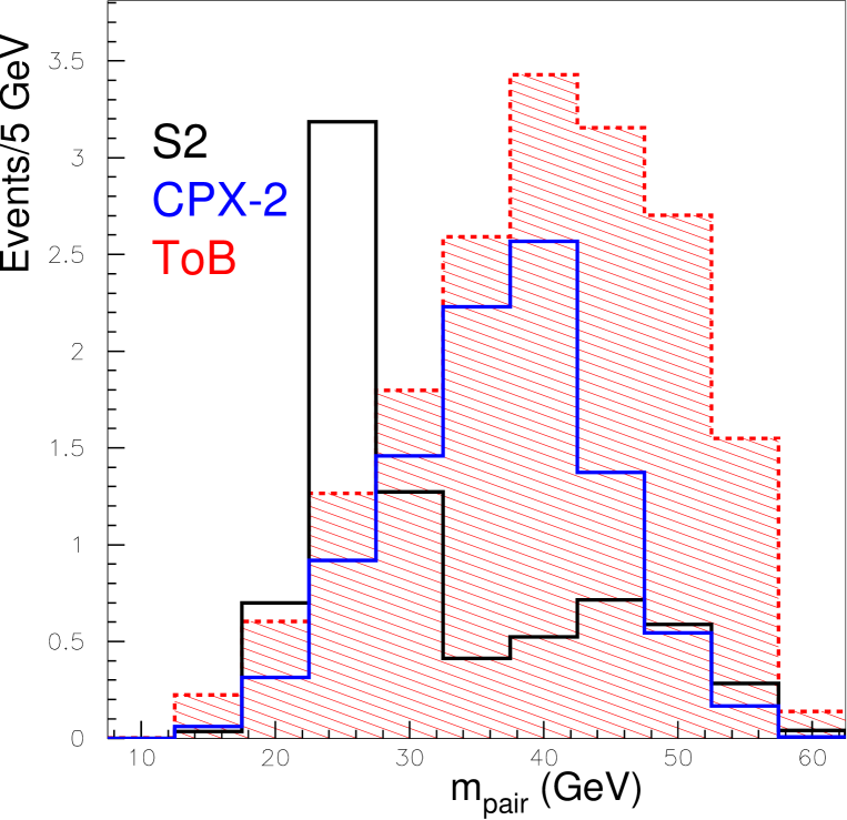
Figure 7: The jet pair invariant mass distribution defined in eq.(7) for signal scenarios S2 and CPX-2 (black and blue or dark grey histograms) and for the total background (shaded histogram) at the LHC. We have applied the acceptance cuts (4), demanding exactly four reconstructed jets, at least three of which are tagged, and required both di–jet invariant masses in the optimal pairing to lie between 10 and 60 GeV. The histograms give the number of events per bin and per 10 fb^-1 of integrated luminosity.

A convincing signal can therefore only be established by detecting characteristic features in some kinematical distributions. To this end we consider the $m_{\rm pair}$ and $m_{4j}$ distributions already discussed for the Tevatron; they are shown in Fig. 7 and 8, respectively. Unfortunately the background shows a peak in the $m_{\rm pair}$ distribution between 30 and 40 GeV, not far from the peak of the signal in the scenarios we consider. A tighter cut on $m_{\rm pair}$ will nevertheless improve the signal–to–background ratio. Moreover, the four–jet invariant mass distribution of the background peaks at large values, largely due to the contribution from $t\bar{t}$ production. At least for scenarios with $h_{2}$ masses in the lower half of the “LEP hole” region a tighter cut on $m_{4j}$ will therefore also improve the significance of the signal.

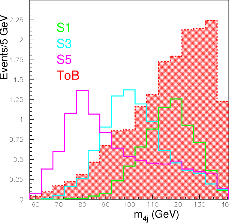
Figure 8: The four–jet invariant mass distribution for signal scenarios S1 (black), S3 (dark blue or dark grey) and S5 (green or light grey) as well as the total background (shaded). We have applied the same cuts of Fig. 7. The histograms give the number of events per bin and per 10 fb^-1 of integrated luminosity.

Scenario	$S$	$B$	${\cal S}$
S1	30.3	23.7	6.22
S2	30.4	19.8	6.83
S3	29.8	16.1	7.43
S4	30.1	12.7	8.45
S5	29.4	9.70	9.44
CPX-1	35.3	21.2	7.66
CPX-2	39.1	29.9	7.15

Table 7: Final number of signal events $S$, background events $B$ and significance ${\cal S}$ at the LHC, defined as ${\cal S}=S/\sqrt{B}$, for 60 fb^-1 of data after all cuts, including the double peak requirement (3).

For our final definition of the significance of the signal we therefore again count the events in the kinematical region defined by the cuts (3). The results are summarized in Table 7, where we assume an integrated luminosity of 60 fb^-1, corresponding to three years of nominal “low luminosity” running with two experiments.

As expected from the last two figures, the significance decreases with increasing $m_{h_{2}}$. This is almost entirely due to the increase of the background with increasing $4j$ invariant mass shown in Fig. 8. The number of signal events after all cuts is almost independent of $m_{h_{2}}$. We saw in Table 6 that scenarios with smaller $m_{h_{2}}$ have larger total cross sections. This is only partially compensated by the increased $b-$tagging efficiency, so that the signal cross section after the cuts considered in Table 6 still decreases with increasing $m_{h_{2}}$. However, Fig. 8 shows that scenarios with smaller $m_{h_{2}}$ also have a longer tail of the $4j$ invariant mass distribution towards large values (but below the upper limit of 140 GeV). This results in a reduced efficiency for the final “double peak” cut, which happens to almost exactly compensate the $m_{h_{2}}$ dependence of the cross section before this cut.

We also see that for given $m_{h_{2}}$, increasing $m_{h_{1}}$ reduces the significance. Recall from table 6 that the signal cross section does not depend much on $m_{h_{1}}$ after the cuts considered there. On the other hand, Fig. 7 again shows poorer efficiency for passing the final “double peak” cut with reduced Higgs mass, since more of the tail towards larger values (now of the averaged di–jet invariant mass) is cut away. However, this Figure also shows an even more rapid increase of the background with increasing $m_{\rm pair}$.

More importantly, Table 7 shows that after the double peak cut, the signal always exceeds the background, giving a final statistical significance of at least 5 standard deviations, and a signal sample of some 30 events.

This result is somewhat at odds with the previous most detailed analysis [9], which used cuts similar to our’s, but did not include showering, hadronization and the underlying event. The absence of showering eliminates all $t\bar{t}$ backgrounds after requiring $m_{4j}<m_{t}$. On the other hand, ref.[9] finds a much larger $W+4b$ cross section (our process p2), and also finds a sizable $W+3b+j$ cross section (our process p3). The latter indicates that these background estimates include processes with $b$ quarks in the initial state; otherwise the cross sections for processes with an odd number of $b$ quarks in the final state would be suppressed by the square of a small CKM matrix element, making them essentially negligible (as in our study). In our treatment these reactions are included in the $W+4b$ background. However, this does not explain the very large $W+4b$ cross section found in ref.[9], 25 fb after cuts, nearly an order of magnitude larger than the 3 fb (see Table 6). Moreover, ref.[9] finds that the $W+4b$ cross section at the LHC after all cuts is more than thousand times larger than at the Tevatron. We find this ratio to be close to 40; this seems more reasonable to us, given that the total $W+4b$ cross section only increases by about a factor of eleven (as does the inclusive $W$ production cross section) when going from the Tevatron to the LHC. On the other hand, process p4, which dominates our $W+4j$ background, has apparently not been included in ref.[9]. Nevertheless our final $S/B$ ratio is more than two times higher than that of ref.[9]. However, since the absence of showering also increases the signal acceptance, the final significance quoted in ref.[9] is actually somewhat higher than our estimate.

5 Conclusions

We analyzed the possibility of observing neutral Higgs bosons at currently operating hadron colliders in the framework of the CP violating MSSM. We explored the $\ell jjjjE\!\!\!\!/_{T}$ channel with double, triple and quadruple $b$ tag, focusing on the region of parameter space not excluded by LEP searches. We have explicitly considered a large number of SM backgrounds, breaking up the generic $W+4j$ QCD backgrounds into many classes, e.g. depending on the number of $b$ quarks in the final state, and carefully treating the production of additional $b\bar{b}$ and $c\bar{c}$ pairs in QCD and $t\bar{t}$ events. We employed a full hadron–level Monte Carlo simulation using the PYTHIA event generator and its PYCELL toy calorimeter. We carefully implemented $b-$tagging, including mistagging of $c-$jets or light flavor or gluon jets.

We first applied this to the Tevatron collider. We found that if we require three tagged jets, we can only expect about one signal event per 10 fb^-1 of integrated luminosity, on a background of about 0.3 events. On the other hand, if we require only double $b-$tag, the signal increases by a factor of about 4, but the background increases by two orders of magnitude, again making the signal unobservable.

Going from the Tevatron to the LHC increases the raw signal cross section by about a factor of 10, whereas some of the important raw background cross sections increase by two orders of magnitude. We therefore have to demand at least three $b-$tags. In contrast to previous analyses [8, 9], we find $t\bar{t}$ production to be the biggest background. This is partly due to the effect of showering. Moreover, we include backgrounds not (explicitly) considered before, in particular $Wb\bar{b}cj$ final states (where $j$ stands for a light quark) which we find to be the dominant non$-t\bar{t}$ background at the LHC. Nevertheless, by focusing on events with exactly four jets, and cutting simultaneously on the average di–jet invariant mass and the four–jet invariant mass, we found a signal rate above the background, and a signal significance exceeding 5 standard deviations for an integrated luminosity of 60 fb^-1. This luminosity could be accumulated at the end of “low luminosity” running of the LHC after summing over both experiments.

Although we improved on earlier analyses in a number of ways, our treatment of $b-$tagging is not fully realistic. We assumed constant (mis)tagging probability for jets within a certain rapidity window and with $E_{T}$ above 15 GeV, and vanishing probability for all other jets. Moreover, we assumed that these probabilities factorize, i.e. can be applied to each jet independent of the rest of the event. More sophisticated tagging algorithms can directly classify the entire event as containing a given (minimal) number of $b-$jets. However, we checked that our simple algorithm reproduces published results for $t\bar{t}$ events at the Tevatron; recall that this is one of our main backgrounds.

Experiments have the possibility to change tagging criteria. This allows to increase the tagging efficiency at the cost of also increasing the mistagging probability. Even if (mis)tagging probabilities indeed factorize, it is not clear that the same parameter choice should be made for all tags. For example, at the Tevatron one might try to combine two strong $b-$tags, similar to the ones we employed, with a weaker one; both the signal rate and the signal to background ratio should then lie between our results for double and triple $b-$tag. Recall, however, that the total number of signal events even with only double $b-$tag is quite small at the Tevatron. We therefore do not think that such more sophisticated tagging algorithms can change our pessimistic conclusion regarding the Tevatron.

However, at the LHC one could increase the signal to background ratio even more by requiring a fourth $b-$tag with softer tagging criteria, possibly simultaneously relaxing the requirement on the number of jets in the event to increase the statistics. This could be used to confirm the existence of a signal. On the other hand, using milder criteria already for the third tagged $b$ is probably not very useful, since the dominant backgrounds contain a $c$ quark which could quite easily be mistagged if too mild tagging criteria are used. The signal can also be corrobated using $Zh_{2}$ production with $Z\rightarrow\ell^{+}\ell^{-}$ [8, 9]. This channel does not receive significant background from $t\bar{t}$ production, so the signal to background ratio should be about two times higher than for the signal we considered. Unfortunately it also has about five times smaller signal rate, leaving only about 2 events per 10 fb^-1 of luminosity at the LHC.

Another concern is the reliability of the background estimates, which are based on leading order QCD calculations. Higher order corrections to the $t\bar{t}$ cross section are known. We did not include them, since our signal calculation also does not include NLO corrections; moreover, NLO corrections to $t\bar{t}$ production are not very large. Since the $W+4j$ cross section is ${\cal O}(\alpha_{S}^{4})$, the leading order estimate suffers from even larger scale uncertainties than the $t\bar{t}$ cross section. An almost complete NLO calculation to $W^{-}+4j$ production became available very recently [29]. They find moderate negative NLO corrections. However, they use a somewhat smaller renormalization and factorization scale; using this scale would e.g. increase our $W+4b$ background by about a factor of 1.8. Moreover, their numerical results are for $\sqrt{s}=7$ TeV, use significantly stronger cuts on the jet transverse momenta and, most importantly, do not distinguish the flavor of the jets; it is not at all clear whether this result carries over to final states containing two, three of four heavy quarks. Recall also that our background requires good control of the tail of the $t\bar{t}$ four–jet invariant mass distribution. A careful validation of background Monte Carlo generators using real data will therefore be essential before a signal can be claimed.

We conclude that searches for $Wh_{2}$ production with $W\rightarrow\ell\nu$ and $h_{2}\rightarrow h_{1}h_{1}\rightarrow b\bar{b}b\bar{b}$ should be able to close that part of the “LEP hole” in parameter space where $h_{1}\rightarrow b\bar{b}$ decays dominate. The same search would also probe parts of the parameter space of many extensions of the MSSM where a heavier Higgs boson can decay into two lighter bosons, each of which in turn decays into a $b\bar{b}$ pair. The search will be challenging, but the prize for a successful search would be well worth the effort: the discovery of not one, but two Higgs bosons at once!

Acknowledgments

We thank A. Datta, S. Fleischmann, R. Frederix, S. Gonzalez, M. Maity, F. Maltoni and J. Schumacher for useful discussion. This work was partially supported by the Bundesministerium für Bildung und Forschung (BMBF) under Contract No. 05HT6PDA, by the EC contract UNILHC PITN-GA-2009-237920, and by the Spanish grants FPA2008-00319, CSD2009-00064 (MICINN) and PROMETEO/2009/091 (Generalitat Valenciana).

References

- [1] For introductions into supersymmetric extensions of the Standard Model in general, and the MSSM in particular, see e.g. M. Drees, R.M. Godbole and P. Roy, Theory and Phenomenology of Sparticles, World Scientific, Singapore (2004); H.A. Baer and X.R. Tata, Supersymmetry: from superfields to scattering events, Cambridge Press (2006).
- [2] A. Pilaftsis, Phys. Rev. D58 (1998) 096010, hep-ph/9803297; Phys. Lett. B435 (1998) 88, hep-ph/9805373. For a recent review, see E. Accomando et al., arXiv:hep-ph/0608079.
- [3] J.S. Lee, A. Pilaftsis, M. Carena, S.Y. Choi, M. Drees, J.R. Ellis and C.E.M. Wagner, Comput. Phys. Commun. 156 (2004) 283 hep-ph/0307377; J.S. Lee, M. Carena, J. Ellis, A. Pilaftsis and C.E.M. Wagner, Comput. Phys. Commun. 180, 312 (2009), arXiv:0712.2360 [hep-ph], and references therein.
- [4] S. Schael et al. (ALEPH, DELPHI L3 and OPAL Collaborations) Eur. Phys. J. C 47 (2006) 547, hep-ex/0602042.
- [5] OPAL Collab., G. Abbiendi et al., Eur. Phys. J. C27 (2003) 311, hep-ex/0206022.
- [6] DELPHI Collab., J. Abdallah et al., Eur. Phys. J. C38 (2004) 1, hep-ex/0410017.
- [7] P. Bechtle, O. Brein, S. Heinemeyer, G. Weiglein and K.E. Williams, Comput. Phys. Commun. 181 (2010) 138, arXiv:0811.4169 [hep-ph].
- [8] K. Cheung, J. Song and Q.-S. Yan, Phys. Rev. Lett. 99 (2007) 031801, hep-ph/0703149.
- [9] M. Carena, T. Han, G.Y. Huang and C.E.M. Wagner, JHEP 0804, 092 (2008), arXiv:0712.2466 [hep-ph].
- [10] S. W. Ham, S. A. Shim and S. K. Oh, Phys. Rev. D 80 (2009) 055009, arXiv:0907.3300 [hep-ph].
- [11] S. Chang, P. J. Fox, and N. Weiner, JHEP 08 (2006) 068, hep-ph/0511250.
- [12] H.-P. Nilles, M. Srednicki and D. Wyler, Phys. Lett. 120B (1983) 346; J.P. Derendinger and C.A. Savoy, Nucl. Phys. B237 (1984) 307; M. Drees, Int. J. Mod. Phys. A4 (1989) 3635; J.R. Ellis, J.F. Gunion, H.E. Haber, L. Roszkowski, and F. Zwirner, Phys. Rev. D39 (1989) 844; U. Ellwanger, Phys. Lett. B303 (1993) 271, hep-ph/9302224.
- [13] S. W. Ham, J. O. Im and S. K. OH, Eur. Phys. J. C58, 579 (2008), arXiv:0805.1115 [hep-ph].
- [14] U. Ellwanger, J.F. Gunion and C. Hugonie, JHEP 07 (2005) 041, hep-ph/0503203.
- [15] M. Carena, J.R. Ellis, A. Pilaftsis and C.E.M. Wagner, Phys. Lett. B 495 (2000) 155, hep-ph/0009212.
- [16] S. Heinemeyer, W. Hollik and G. Weiglein, Comput. Phys. Commun. 124 (2000) 76, hep-ph/9812320; M. Frank, T. Hahn, S. Heinemeyer, W. Hollik, H. Rzehak and G. Weiglein, JHEP0702, 047 (2007), hep-ph/0611326.
- [17] H.L. Lai, J. Huston, S. Kuhlmann, J. Morfin, F. Olness, J.F. Owens, J. Pumplin and W.K. Tung, Eur. Phys. J. C12 (2000) 375, hep-ph/9903282.
- [18] F. Maltoni and T. Stelzer, JHEP 0302, 027 (2003).
- [19] Particle Data Group, C. Amsler et al., Phys. Lett. B667 (2008) 1.
- [20] T. Sjostrand, S. Mrenna and P. Skands, JHEP 0605, 026 (2006).
- [21] CDF IIb Collaboration, P. T. Lukens, The CDF IIb detector: Technical design report, . FERMILAB-TM-2198.
- [22] K. Hanagaki [D0 Collab.], FERMILAB-CONF-05-647-E; C. Neu [CDF Collab.], FERMILAB-CONF-06-162-E; T. Wright [CDF and D0 Collabs.], arXiv:0707.1712 [hep-ex].
- [23] D. Acosta et al., Phys. Rev. D 71 (2005) 052003.
- [24] T. Hahn, S. Heinemeyer, F. Maltoni, G. Weiglein, and S. Willenbrock, SM and MSSM Higgs boson production cross sections at the Tevatron and the LHC, hep-ph/0607308.
- [25] The Atlas Collab., CERN-LHCC-99-15, ATLAS-TDR-15 (1999).
- [26] G. Aad et al. [The ATLAS Collaboration], arXiv:0901.0512 [hep-ex].
- [27] M. Lehmacher, arXiv:0809.4896 [hep-ex].
- [28] E. Alagoez et al., http://unizh.web.cern.ch/unizh/Activities/cms.htm.
- [29] C.F. Berger et al., arXiv:1009.2338 [hep-ph].
- [30] T. Han and S. Willenbrock, Phys. Lett. B273 (1991) 167–172.
- [31] M. L. Ciccolini, S. Dittmaier, and M. Krämer, Phys. Rev. D68 (2003) 073003, hep-ph/0306234.