Multivariate discrimination and the Higgs+W/Z search

Abstract:

A systematic method for optimizing multivariate discriminants is developed and applied to the important example of a light Higgs boson search at the Tevatron and the LHC. The Significance Improvement Characteristic (SIC), defined as the signal efficiency of a cut or multivariate discriminant divided by the square root of the background efficiency, is shown to be an extremely powerful visualization tool. SIC curves demonstrate numerical instabilities in the multivariate discriminants, show convergence as the number of variables is increased, and display the sensitivity to the optimal cut values. For our application, we concentrate on Higgs boson production in association with a $W$ or $Z$ boson with $H\to{b\bar{b}}$ and compare to the irreducible standard model background, $Z/W+{b\bar{b}}$. We explore thousands of experimentally motivated, physically motivated, and unmotivated single variable discriminants. Along with the standard kinematic variables, a number of new ones, such as twist, are described which should have applicability to many processes. We find that some single variables, such as the pull angle, are weak discriminants, but when combined with others they provide important marginal improvement. We also find that multiple Higgs boson-candidate mass measures, such as from mild and aggressively trimmed jets, when combined may provide additional discriminating power. Comparing the significance improvement from our variables to those used in recent CDF and DØ searches, we find that a 10-20% improvement in significance against $Z/W+b\bar{b}$ is possible. Our analysis also suggests that the $H+W/Z$ channel with $H\to{b\bar{b}}$ is also viable at the LHC, without requiring a hard cut on the $W/Z$ transverse momentum.

1 Introduction

Search strategies for new physics often depend on being able to find a small signal on top of a large background. In many cases, there are an enormous number of possible discriminants which one would ideally like to combine to maximize search sensitivity. One approach is to choose, by some means, a small set of well-understood and fairly uncorrelated variables and feed them into a multivariate discriminant such as an Artificial Neural Network (ANN) or a Boosted Decision Tree (BDT). This approach has been applied productively in the light Higgs boson searches at CDF [1] and DØ [2, 3]. While these multivariate techniques can often improve discrimination power, it is almost impossible to follow their inner workings in full detail. A major concern is that they can pick up on unphysical features of the Monte Carlo samples used to train them, rather than real differences in the signal and background processes. At the same time, it is also unclear how dependent the absolute performance and robustness are on the initial choice of variables. While we generally expect that there are important multidimensional correlations that a computer can find better than a person, we would like to be able to capitalize on this fact in a more systematic manner. The goal of this paper is to develop such a systematic programme, showing how to produce combined discriminants that are more trustworthy and better optimized. Kinematic observables based on well-understood, hard, perturbative physics become our 4-5 most powerful discriminants. Beyond that, it is useful to examine properties of the jets themselves affected by perturbative QCD emissions.

The main example we consider is the production of a Higgs boson at the 14 TeV LHC in association with a vector boson ($Z$ or $W$), with the Higgs decaying to ${b\bar{b}}$. This process was studied by both ATLAS and CMS. ATLAS, for example, concluded that the most promising channel, $WH\to\ell\nu b\bar{b}$, would not provide enough significance for discovery [4]. More recently, $WH$ and $ZH$ were revived with the observation that putting a hard cut on a single variable can significantly enhance signal-to-background ratio [5, 6]. In particular, imposing a cut $p_{T}>200$ GeV on the reconstructed $Z$ reduces the signal by factor of 20, but reduces the background by a much larger factor of 320. This $p_{T}$ cut (used in conjunction with jet substructure methods to optimize mass resolution and background shaping), reinstated $WH$ and $ZH$ as possible Higgs discovery modes at the LHC. It is, at the outset, unclear whether a multivariate approach would pick up on the fact that a hard cut on $p_{T}$ could make $ZH$ or $WH$ viable. It is also unclear whether the hard $p_{T}$ cut is optimal, or whether better use could be made of the 95% of $ZH$ signal events which this cut throws out. We seek to optimize multivariate searches for the standard model Higgs boson at the Tevatron and LHC.

With this motivation, our goal is to analyze systematically the entire phase space of $ZH$ production with $H\to b\bar{b}$ to find the kinematic regions that maximize signal significance. We will concentrate on separating $ZH\to\ell^{+}\ell^{-}b\bar{b}$ from its irreducible background in the standard model, for example, from $pp\to Zb\bar{b}\to\ell^{+}\ell^{-}b\bar{b}$. Here, $\ell$ is an electron or muon. We will also require the $b$’s to appear in separate jets. This dijet reconstruction approach continues to work well at high Higgs boson $p_{T}$ (up to about 400 GeV). We note that our results are complementary to any further improvements achievable using substructure-based techniques. We will only briefly discuss the reducible backgrounds, such as mis-tagged $b$-jets. All of these other backgrounds account for less than half of the total background at CDF LABEL:cdfnote10235. We will also show results for the $WH$ channel as compared to its irreducible $\ell\nu{b\bar{b}}$ background. For both $ZH$ and $WH$, the reducible backgrounds are clearly important to establish the final search reach, but restricting to irreducible backgrounds more concisely illustrates our main observations.

Our first step is to develop and study a very broad range of single-variable discriminants. We consider initially thousands of discriminants, including kinematic observables corresponding to the “hard scattering” (e.g. $\Delta\eta$ between the $b$ jets, $\hat{s}$, etc.) along with observables that distinguish signal from background due to differences in the QCD radiation patterns (e.g. color connections, subjet multiplicities, etc.). Some of these variables, such as twist and pull, are more generally applicable. We also at varying the jet sizes and jet algorithm, and the effect of trimming [8]. Many of the variables are very similar, but enough are sufficiently independent to be considered separately.

Once the input variables are cataloged, we establish a criterion to evaluate their usefulness. The ultimate measure is, of course, how much integrated luminosity the collider would need to find (or reject) a hypothesized signal to a certain statistical significance, say $5\sigma$. Even with this criterion, there are multiple measures of significance — should we compare the events in a single optimized signal bin to the Monte Carlo prediction for signal and background? Should we look for an excess in the signal region compared to the sidebands? Should we fit curves and compare the $\chi^{2}$ for various simulated distributions? How do we treat the experimental systematic uncertainties? In fact, it is nearly impossible to get an accurate measure of the final search reach from a theoretical study without collaboration-approval-dependent full detector simulation. Nevertheless, the relative importance of different discriminants should be roughly independent of the final search strategy. We therefore argue that the Significance Improvement Characteristic (SIC), defined as the signal efficiency divided by the square root of background efficiency resulting from a cut on a given discriminant,

$${\text{\sc SIC}}\equiv\frac{\varepsilon_{S}}{\sqrt{\varepsilon_{B}}},$$ (1)

is a practical and useful measure. We will show that this quantity, viewed as a function of $\varepsilon_{S}$ allows us to efficiently explore the convergence and limitations of the multivariate combinations. One can also use the maximum of SIC, $\overline{\text{\sc SIC}}$, to rank variables and as a quantitative measure of final efficiency.

This paper is organized as follows: Section 2 describes the selection cuts we use for the signal and background samples, and the resulting cross sections. We only consider irreducible backgrounds, so the numbers present do not directly translate into a discovery potential. In Section 3, we describe our single variable discriminants. This section includes variables which are useful at the hard parton level, such as jet $p_{T}$’s, physically motivated variables, such as helicity angles, variables dependent on the radiation pattern, such as pull [9], and some useful variables that do not have an obvious physical motivation as well. Section 4 discusses some efficiency measures and motivates the SIC curves. Section 5 gives a brief introduction to some of the multivariate measures we consider, and explains some features of boosted decision trees (BDTs), our method of choice. Section 6 describes improvements when variables are combined and our algorithm for finding the optimal set. We show that in the case of associated Higgs boson production the SIC curves for Boosted Decision Trees continue to increase in performance until the of 6^th or 7^th variable is added. The addition of more variables does not provide additional discrimination — it does not improve the SIC. The efficiencies used in these sections are all based on samples constrained to lie within a fixed Higgs mass window using a particular jet algorithm. We justify this window and algorithm in Section 7. Section 7 also shows that additional improvement may result from combining multiple measures of the ${b\bar{b}}$ invariant mass, from different jet algorithms. For the final discriminants the mass window is removed and ${m_{b\bar{b}}}$ is included in the multivariate analysis. Section 8 shows the final discriminant combinations for the Tevatron and the LHC. A summary and discussion is presented in Section 9.

2 Event Generation

The bulk of this paper will refer to a reference sample of events generated initially with madgraph v4.4.26 [11]: $pp\to ZH\to\ell^{+}\ell^{-}{b\bar{b}}$ for signal and $pp\to Z{b\bar{b}}\to\ell^{+}\ell^{-}{b\bar{b}}$ for background at $\sqrt{S}$=14 TeV. These are then showered through pythia v8.140 [12]. Jets are reconstructed using fastjet v2.4.2 [13], and these (along with the leptons) serve as our “detector-level” objects. The multivariate analysis is done using the tmva v4.0.4 package [16] that comes with root v5.27.02 [17]. Our reference Higgs boson mass is $m_{H}=120$ GeV throughout: above the LEP limit of 115 GeV but below 130 GeV where $b\bar{b}$ decay no longer dominates. Masses below 115 GeV are excluded by LEP, and decay to $WW^{*}$ starts to dominate above around 135 GeV [14]. We will also consider $ZH$ events at the Tevatron $p\bar{p}$ with $\sqrt{S}=1.96$ TeV, and $WH$ events at the Tevatron and LHC. The $WH$ events will be compared to their $W{b\bar{b}}$ irreducible backgrounds. Reducible backgrounds such as $Wjj$ with false $b$-tags or $t\bar{t}$ will not be considered, for simplicity.

Generator-level cuts are described in Table 1. It is important that the cuts applied at the hard parton level, in madgraph, not be as tight as the cuts used for the final jets. We found that a factor of 2 margin was wide enough while maintaining acceptable generation efficiency. We did not apply a cut on ${m_{b\bar{b}}}$ in the generated samples. Once this sample is generated and showered, we require two $b$-tagged jets. Our operative definition of $b$-tagging matches $B$-hadrons from the intermediate event record to final-state jets with $\Delta R_{jB}$ smaller than the jet clustering radius. We then cut on the $b$-jet $p_{T}$ and rapidity.

hard-parton level cuts	detector level cuts
$p_{T}^{b}>7$ GeV	$p_{T}^{b}>15$ GeV
$p_{T}^{\mu}>3$ GeV	$p_{T}^{\mu}>6$ GeV
$p_{T}^{e}>3$ GeV	$p_{T}^{e}>20$ GeV (LHC), $10$ GeV (Tevatron)
$|\eta_{b}|<5$ and $|\eta_{\ell}|<5$	$|\eta_{b}|<2.5$ and $|\eta_{\ell}|<2.5$

Table 1: Cuts applied for event generation.

We generated 3 million signal events and 30 million background events. After $b$-tagging and detector cuts were applied, we were left with around 2M signal and 4M background events. Within our fiducial Higgs Mass Window of $90\,\mathrm{GeV}<{m_{b\bar{b}}}<124\,\mathrm{GeV}$, we ended up with 1.5M signal and 0.6M background simulated events. This specific window will be justified later as the one that maximizes significance.

	LHC (14 TeV)		Tevatron (1.96 TeV)
Integrated Luminosity, $\int\!\mathscr{L}$	30 $fb^{-1}$		10 $fb^{-1}$
	$pp\rightarrow ZH$	$pp\rightarrow Zb\bar{b}$	$p\bar{p}\rightarrow ZH$	$p\bar{p}\rightarrow Zb\bar{b}$
$\sigma$ times Branching Ratio	33.4 fb	57,200 fb	3.63 fb	1250 fb
After Generator-Level Cuts	31.5 fb	26,000 fb	3.40 fb	570 fb
Two $b$ Tags % (of Gen-Level)	57%	25%	81%	25%
Higgs Mass Window % (of Gen-Level)	40%	4%	52%	3%
Initiated by $gg$ (as opposed to $q\bar{q}$)	0%	90%	0%	27%
Xsec (in Higgs Mass Window)	12.3 fb	1100 fb	1.8 fb	14.9 fb
Events (Xsec $\times\int\!\mathscr{L}$)	370	33,700	18	149
Starting $B/S$	91.1		8.2
Starting $S/\sqrt{B}$	2.02		1.47

Table 2: Cross Sections for LHC and Tevatron signal and background. The lowest 6 rows refer to a Higgs mass-window cut, $90\,\mathrm{GeV}<{m_{b\bar{b}}}<124\,\mathrm{GeV}$, where the mass is computed from the hardest two $b$-tagged $R\!=\!0.5$ anti-$k_{T}$ jets. The significances here will be the baseline references from which we compute fractional improvements. This applies even for samples without an ${m_{b\bar{b}}}$ cut where different ${m_{b\bar{b}}}$ measures are used as part of a multivariate discriminant.

The overall cross sections and efficiencies for these cuts are shown in Table 2. The row in this table labeled “Higgs Window %” refers the percent of events with  (a window we find later to be optimal, see Section 7 below). For this table, jets are found using the anti-$k_{T}$ algorithm with $R\!=\!0.5$ and ${m_{b\bar{b}}}$ is the invariant mass of the two $b$-tagged jets in the event. The “Xsec” row, and the rows below, provide cross sections and a normalization for the initial significance. These are all after the ${m_{b\bar{b}}}$ mass window cuts, but with no other discriminating variable applied. Our improvements will be compared to this significance. We will later treat the mass window in a more sophisticated way, combining multiple mass measures and jet algorithms. Here find it pedagogically useful to have a standard set of reference efficiencies.

The row in the table labeled “Initiated by $gg$”, which is also for events within the ${m_{b\bar{b}}}$ window, shows an important distinction between the Tevatron and the LHC. Note that the signal is all $q\bar{q}$ initiated at both machines. Since the $Z{b\bar{b}}$ background at the LHC is mostly $gg$ initiated it will be easier to distinguish from signal than the backgrounds at the Tevatron, which are mostly $q\bar{q}$-initiated, and therefore more similar to the signal.

3 Single Variable Discriminants

In this section we catalog all of the variables we use as potential discriminants between signal and background. The language will refer to the $ZH\to\ell^{+}\ell^{-}{b\bar{b}}$ process, although the same variables can be used for the $WH$ sample with $\ell\nu$ replacing $\ell^{+}\ell^{-}$. The variables will be split roughly into two classes, kinematic and radiation. Kinematic variables are those which are meaningful at the hard parton-level, such as ${m_{b\bar{b}}}$. They are expressible in terms of the 4-momenta of the $\ell^{+}$, $\ell^{-}$, $b$, and $\bar{b}$. Although the kinetic variables can be defined at the parton level, we will measure them using the $b$-jet momenta. Radiation variables, such as the number of charged hadrons in a jet, are those which result mainly from QCD radiation. In the Monte Carlo, these variables are populated due to the parton shower.

To begin, consider how many independent degrees of freedom there are at the hard parton level. We will treat showering and initial state radiation later. The underlying hard process we are interested in is $pp\to ZH\to\ell^{+}\ell^{-}{b\bar{b}}$. The final state is characterized by the 4-momenta of the four final state particles, which is 12 degrees of freedom including the mass-shell constraints of the $b$’s and leptons. One approach to constructing discriminants is to simply throw the 12 degrees of freedom, $p_{b}^{x},p_{b}^{y},p_{b}^{z}$, etc., into a multivariate analysis and hope for the best. However, it makes more sense to consider physically motivated variables. Azimuthal rotation invariance, and the overall $\vec{p}_{T}=0$ constraint reduce the physical degrees of freedom to 9, and $Z$ and $H$ invariant mass constraints reduce the number down to 7. Since there are multiple ways physics can motivate the choice of variables, this will result in many more than 7 variables. We use the standard coordinate system with $\pm\hat{z}$ pointing in the beam direction, $y$ is the rapidity, $\eta$ is the pseudorapidity, and $\phi$ is the azimuthal angle.

We first consider variables which are natural from the experimental point of view. These include things like transverse momenta, invariant masses, rapidity differences, angular separations, etc.. These will be cataloged in Section 3.1. This can be thought of as a type of bottom-up parametrization. The alternative is a top-down parametrization, motivated by the physical process. One can start with variables that characterize the $ZH$ production, such as $\hat{s}$ and the production polar angle $\theta^{\star}$. Then when the Higgs and $Z$ decay, one can think about various angles constructed from their decay products in their rest frame. This approach will lead to variables discussed in Sections 3.2 and 3.3. Combining the bottom-up and top-down ways of thinking leads to an even larger set of possible discriminants, discussed in Section 3.4. Sections 3.5 to 3.10 describe some of the showered variables.

3.1 Lab-frame Kinematical Variables

First, consider variables which are natural to define and measure in the lab-frame. Using only the 4-momenta of the $b$ jets in the lab frame, we have

• $p_{T}$ of the two $b$’s: $p_{T}^{b1}$ for the higher-$p_{T}$, and $p_{T}^{b2}$ for the lower-$p_{T}$ one

• $\Delta\eta_{{b\bar{b}}}=\eta_{b}-\eta_{\bar{b}}$

• $\Delta\phi_{{b\bar{b}}}=\phi_{b}-\phi_{\bar{b}}$   (properly wrapped to have a range between $-\pi$ and $\pi$)

• $\Delta R_{{b\bar{b}}}=\sqrt{(\Delta\eta_{{b\bar{b}}})^{2}+(\Delta\phi_{{b\bar{b}}})^{2}}$

The same variables are also considered for the lepton system, with $\ell^{+}$ and $\ell^{-}$ replacing the ${b\bar{b}}$. There, one can also treat the positively and negatively charged leptons separately, although we found that sorting by $p_{T}$, as with the $b$’s, tends to work better.

There are variables involving the reconstructed Higgs boson with four-momenta $p_{H}^{\mu}=p_{b}^{\mu}+p_{\bar{b}}^{\mu}$, and reconstructed $Z$, with $p_{Z}^{\mu}=p_{\ell^{+}}^{\mu}+p_{\ell^{-}}^{\mu}$:

• $p_{T}^{Z}$ and $p_{T}^{H}$, the $p_{T}$ of the $Z$ and Higgs boson. At the parton-level these are the same, but they end up slightly different due to jet reconstruction.

• $p_{T}^{CM}$: Center of Mass $p_{T}$, the magnitude of the vectorial sum of the 2 $b$-jet and 2 lepton $p_{T}$’s. This is zero for the parton-level process, but non-zero after showering and jet reconstruction. $p_{T}^{CM}$ is not included in our analysis, as discussed below in the missing $E_{T}$ section.

We show a set of these variables in Figure 1. Some of these, such as $\Delta\eta_{b\bar{b}}$, look to provide very good discriminants. All of the variables are shown for anti-$k_{T}$ $R\!=\!0.5$ jets [15]. Iterative jet algorithms, including anti-$k_{T}$ jets are defined by first assigning all energy depositions into their own protojet. At each stage of the clustering, calculate the distance between each pair of protojets, defined by

$$d_{ij}=min(k_{t_{i}}^{2p},k_{t_{j}}^{2p})\frac{\Delta_{ij}^{2}}{R^{2}},$$ (2)

along with the beam distance of each protojet, defined by

$$d_{iB}=k_{t_{i}}^{2p},$$ (3)

where $\Delta_{ij}^{2}=(y_{i}-y_{j})^{2}+(\phi_{i}-\phi_{j})^{2}$ and $k_{ti}$, $y_{i}$, and $\phi_{i}$ are the transverse momentum, rapidity, and azimuth of protojets $i$ and $j$. The parameter $p=1$ for the $k_{T}$ algorithm, $p=0$ for the Cambridge/Achten algorithm, and $p=-1$ for the anti-$k_{T}$ algorithm. When one of the distances between protojets is the smallest, those protojets are combined into another protojet by adding their 4-vectors. When one of the beam distances is the smallest, that protojet gets promoted to a real jet and removed from further consideration. Either way, all distances are computed again for the new set of protojets, and the process repeats until all protojets have been promoted.

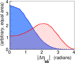
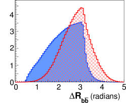
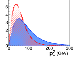
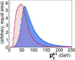
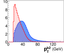
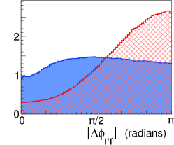
Figure 1: Some lab-frame kinematic variables for $ZH$ signal (solid blue) and $Zb\bar{b}$ background (hashed red) at the LHC. Events satisfy selection cuts and the Higgs mass window cut, $90\,\mathrm{GeV}<{m_{b\bar{b}}}<124\,\mathrm{GeV}$. Horizontal axes are in radians or GeV as appropriate, and vertical axes are in arbitrary units with signal and background normalized to the same area.

Some other variables inspired by previous Higgs boson searches include:

• acoplanarity = $\left|\pi-|\Delta\phi_{b\bar{b}}|\right|+\left|\pi-\Sigma\theta_{b\bar{b}}\right|$. Also for $\ell^{+}\ell^{-}$.

• $m_{T}^{b\bar{b}}={m_{b\bar{b}}}^{2}+p_{x}^{2}+p_{y}^{2}$: transverse mass of ${b\bar{b}}$ system. Also for $\ell^{+}\ell^{-}$.

• $m_{\ell\ell b}$: invariant mass of the $Z$ combined with a $b$-jet. The max or min over the two $b$’s can also be used.

• $p_{T}^{\mathrm{imbalance}}=|\vec{p}_{T}^{b1}+\vec{p}_{T}^{b2}+\vec{p}_{T}^{\ell}-\vec{p}_{T}^{\nu}$—, for the $WH$ search.

3.2 Twist

\psfrag{qqHZbbll}{\!\!\!\!\!\!\!Higgs Boson Signal}\psfrag{ggZbbll}{Background Initiated by $gg$}\psfrag{b/bbar dEta}{$\Delta\eta_{b\bar{b}}$}\psfrag{b/bbar dPhi}{$\Delta\phi_{b\bar{b}}$}\includegraphics[height=144.54pt]{b_bbar_dPhi_vs_b_bbar_dEta_50_new}

Figure 2: $\Delta\eta_{b\bar{b}}$ vs $\Delta\phi_{b\bar{b}}$ for the Higgs boson signal (left) and the $gg$ initiated $Zb\bar{b}$ background dominant at the LHC (right). This is at the hard parton level, and for $p_{T}^{H}>50$ GeV. The difference is less dramatic for lower $p_{T}$ or for the Tevatron, where the $q\bar{q}$-initiated background dominates. Absolute values could also be taken for $b$ indistinguishable from $\bar{b}$.

Signal-Like Twist $\tau=\pi/2$	Background-Like Twist $\tau=0$

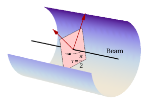
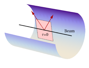
Figure 3: Twist angle $\tau$ in 3D with the $b$ and $\bar{b}$ emerging from the interaction point. The twist angle is defined to be boost invariant and does not exactly correspond to the physical rotation angle of a plane. The case shown, however, has no longitudinal boost.

The strength of the ${b\bar{b}}$ angle discriminants $\Delta\eta$, $\Delta\phi$ and $\Delta R$, motivates us to explore the ${b\bar{b}}$ system more carefully. Figure 2 shows the two-dimensional distribution of parton-level events in the $(\Delta\eta,\Delta\phi)$ plane for the signal and background. It is clear from these plots that the polar angle, which we call twist, would be a good discriminant. If we think of $(\Delta\eta,\Delta\phi)$ as 2D Cartesian coordinates, then polar coordinate combinations are the familiar $\Delta R=\sqrt{\Delta\eta^{2}+\Delta\phi^{2}}$, and the twist angle:

$$\tau\equiv\tan^{-1}\frac{\Delta\phi}{\Delta\eta}\,.$$ (4)

Twist is a longitudinal-boost-invariant version of the rotation of the $H/b/\bar{b}$ plane with respect to the $beam/H$ plane. This is illustrated in Figure 3. The twist angle is zero when the particles are separated along the cylinder in $\eta$, and $\pi/2$ when separated around the cylinder in $\phi$.

The shape of the signal and background twist distributions in Figure 2 can be understood as follows. For low Higgs $p_{T}$, $p_{T}^{H}\ll m_{H}$, the signal lives in bands clustered along $|\Delta\phi|\sim\pi$, and hence $\tau\sim\pi/2$. For $p_{T}\mathrel{\hbox to0.0pt{\lower 4.0pt\hbox{\hskip 1.0pt$\sim$}\hss}\raise 1.0pt\hbox{$>$}}m_{H}$, the signal lives in a ring of $\Delta R\sim 2m_{H}/p_{T}$, and twist is a powerful variable orthogonal to the radial direction. For higher $p_{T}$, the signal becomes somewhat more uniformly distributed in twist, but still retains its $\tau=\pi/2$ preference. This is all purely a consequence of the spherically-symmetric Higgs boson decay boosted transverse to the beam. In contrast, for the background, in particular the $gg$-initiated background, there is a bias for one of the $b$’s to have large rapidity, which leads to low twist. This stems from $t$-channel type singularities in the $Zb\bar{b}$ production matrix elements (in the limit of massless $b$’s.) At higher $p_{T}$, the background retains much of its $\tau=0$ preference. The distributions in Figure 2 reflect an admixture of the high and low $p_{T}$ twist behaviors, biased towards the low $p_{T}$ behavior, which is where most of the events lie.

We show in Figure 4 the twist distributions for signal and background for the ${b\bar{b}}$ system and the $\ell^{+}\ell^{-}$ system. The top panels show the twist distributions at the madgraph level before showering and cuts, and the bottom panels after jets are reconstructed and detector level cuts have been been applied. We can see that the discriminating power of twist for the ${b\bar{b}}$ system is reduced by requiring relatively central jets with a minimal $p_{T}$. However, the background’s bias towards the beam is still evident, and twist still provides a useful discriminant which we will incorporate into our multivariate analysis. Because of its physical motivation, we also suspect the twist angle could have much wider applicability than to the $ZH$ and $WH$ searches we consider here.

Madgraph hard parton level with no cuts
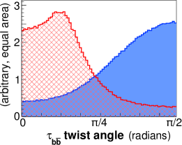
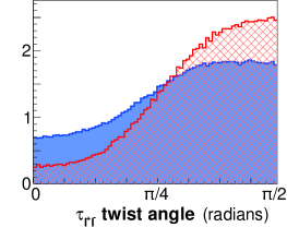
Showered and jetted, with detector cuts

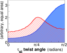
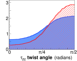
Figure 4: Twist angle distributions for $ZH$ signal (solid blue) and $Z{b\bar{b}}$ background (hashed red), for the LHC with no $p_{T}^{Z}$ cut. Madgraph hard parton-level with no cuts (top) and showered jet-level with detector cuts (bottom). Both are shown only in the Higgs mass-window, $90\,\mathrm{GeV}<{m_{b\bar{b}}}<124\,\mathrm{GeV}$. Vertical axes are in arbitrary units with signal and background normalized to the same area.

3.3 Helicity and Azilicity Angles

Next, we begin to consider variables motivated by the on-shell decays of the Higgs and the $Z$. In their rest frames, each decay is parametrized only by two angles $\theta$ and $\phi$. Since the Higgs boson is a scalar, its decay products are spherically symmetric and therefore distributed uniformly in $\phi$ and $\cos\theta$. Specifically, in the rest frame of the scalar Higgs, the $b$ and $\bar{b}$ quarks travel in opposite directions with a fixed energy ($m_{H}/2$, up to $b$ mass corrections). The rest frame of any fake Higgs boson formed by two $b$-jets will also have two oppositely-going $b$’s in the ${b\bar{b}}$ center-of-mass frame. If we impose that ${m_{b\bar{b}}}$ be close to the Higgs mass, in this frame, the background $b$’s will have energies close to $m_{H}/2$ just like the signal, but they will not be distributed in a spherically symmetric way.

Parameterizing the $H$ decay with two polar angles requires a convention for the axes. Our convention is motivated by the helicity angle used in $W$ and top studies [19]. The angles are constructed in the rest frame of the Higgs boson, and refer to directions defined by the $Z$ and beam 3-momenta observed in this frame. We choose “latitude” to be measured by the helicity angle, $\theta$, with the south pole ($\theta=\pi$) defined to be the direction aligned with the $Z$ (equivalently, the direction along which the $ZH$ parent CM system moves). Given this angle, we still have the freedom to chose any direction perpendicular to the axis as the $\phi=0$ direction. We chose $\phi=0$ to be pointing toward the beam which was moving along $+\hat{z}$ in lab frame coordinates. The QCD background will favor $\phi=0$ and $\phi=\pi$. With this convention, we call longitude the azilicity angle, since it is the azimuthal $\phi$ angle on the sphere whose north pole is defined when the helicity angle vanishes. Azilicity is equivalently the angle between the Higgs boson decay plane and the $ZH$ production plane (constructed with reference to the beams) as viewed in the event’s center of momentum frame. Since $b$ and $\bar{b}$ are indistinguishable, this angle can be chosen to go between $0$ and $\pi/2$. A cartoon of these angles is shown in Figure 5.

\psfrag{b}{$b$}\psfrag{bb}{$\bar{b}$}\psfrag{e}{$\ell$}\psfrag{H}{$H$ boost direction}\psfrag{Z}{$Z$ direction}\psfrag{BM}{beam}\psfrag{AZ}{$\phi_{a}$}\psfrag{TH}{$\theta_{h}$}\includegraphics[height=144.54pt]{angles_higgs_new}

Figure 5: Helicity angle $\theta_{h}$ and azilicity angle $\phi_{a}$ for $H\rightarrow b\bar{b}$. Angles can also be defined for the leptons on the $Z\rightarrow\ell^{+}\ell^{-}$ side of the event.

The helicity and azilicity angles offer the promise of very strong discrimination power, because they are directly tied to physical features of the signal. Indeed, in the top row of Figure 6, we can see that, at the parton-level with no cuts, there are strong singularities at both $\theta=0$ and $\phi=0$ for the background, while the signal distributions are flat, as expected. Detector observability cuts remove the most singular background contributions, but still lead to distributions that show some remaining discriminating power.

Madgraph hard partons with no cuts:
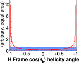
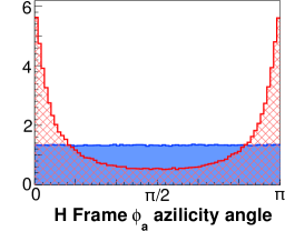
Showered and reconstructed, with detector cuts:

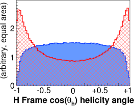
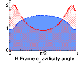
Figure 6: Helicity angle $\theta$ and azilicity angle $\phi$ for the $b$ in the Higgs boson rest frame, for $ZH$ signal (solid blue) and $Z{b\bar{b}}$ background (hashed red) at the LHC. Madgraph hard parton-level with no cuts (top) and showered jet-level with detector cuts (bottom). Both are shown only in the Higgs mass-window, $90\,\mathrm{GeV}<{m_{b\bar{b}}}<124\,\mathrm{GeV}$.

3.4 Kinematic variable construction

We have described a number of variables constructed out of the 4-momenta of the jets and leptons in various frames. There are large combination of variables which can be formed from the measurable kinematic variables. However, using physically motivated variables can help the automated process in the right direction. By searching for useful combinations up front, a neural network, for example, does not have to “discover” how to take an invariant mass or boost to the Higgs boson rest frame.

Thus, we now consider various unintuitive combinations of variables. The procedure is:

• Pick a particle: high-$p_{T}$ $b$-jet, low-$p_{T}$ $b$-jet, high-$p_{T}$ lepton, low-$p_{T}$ lepton, Higgs, $Z$.

• Optionally transform to a boosted frame: Higgs, $Z$, System Center of Mass (CM).

• Optionally rotate the polar axis to point along the initial direction of the particle whose frame you are in (as for helicity and azilicity angles).

• Pick a kinematic property: $p_{T}$, $\eta$, $\phi$, $\cos(\theta)$, etc..

• Optionally pick a second particle to form a sum or difference, sometimes with a coordinate transformation as in $\Delta R$ and twist $\tau$, and sometimes with a more complicated combination as in invariant-mass.

• For vector quantities, optionally take the magnitude of vector sums, $|\vec{p}_{1}\pm\vec{p}_{2}|$ or scalar sums, $|\vec{p}_{1}|\pm|\vec{p}_{2}|$.

Some stranger kinematic variables that prove to be useful in the multi-variable analysis include:

• $\Sigma p_{T}^{b\bar{b}}=|\vec{p}_{T}^{\,b1}|+|\vec{p}_{T}^{\,b2}|$: Sum of magnitudes of $p_{T}$’s of the two b-jets.

• $\Sigma p_{T}^{b1,\ell 2}=|\vec{p}_{T}^{\,b1}|+|\vec{p}_{T}^{\,l2}|$: Sum of magnitudes of $p_{T}$’s of the higher-$p_{T}$ $b$-jet and the lower-$p_{T}$ lepton.

• $\Delta p_{T}^{Z,\ell 1}=|\vec{p}_{T}^{\,Z}|-|\vec{p}_{T}^{\,l1}|$: Difference in magnitude of $p_{T}$ between $Z$ and higher-$p_{T}$ lepton.

• $\Delta p_{T}^{b1,\ell 2}=|\vec{p}_{T}^{\,b1}|-|\vec{p}_{T}^{\,l2}|$: Difference in magnitude of $p_{T}$ between higher-$p_{T}$ $b$-jet and lower-$p_{T}$ lepton.

• $\Delta\eta_{b1,\ell 2}$: Difference in $\eta$ between the higher-$p_{T}$ $b$-jet and the lower-$p_{T}$ lepton.

• $\Delta y_{H,b1}$ and $\Delta y_{H,b2}$: Difference in rapidity between $H$ and higher-$p_{T}$ or lower-$p_{T}$ $b$-jet.

• $\cos(\theta^{*}_{b2})$: Center of Mass frame $\cos(\theta)$ of the lower-$p_{T}$ $b$-jet. Same for higher-$p_{T}$ $b$-jet.

We show the distributions for a number of these Menu-Method variables in Figure 7.

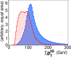
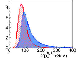
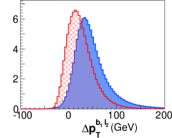
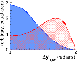
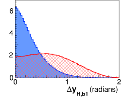
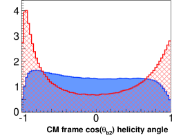
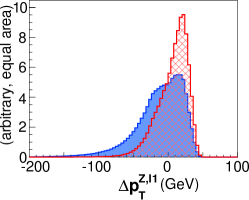
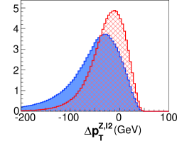
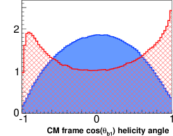
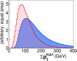
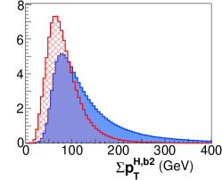
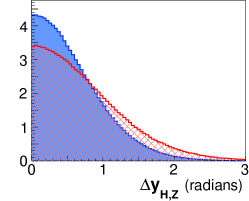
Figure 7: A selection of various variable distributions for $ZH$ signal (solid blue) and $Zb\bar{b}$ background (hashed red) at the LHC. Events satisfy selection cuts and the Higgs mass-window cut, $90\,\mathrm{GeV}<{m_{b\bar{b}}}<124\,\mathrm{GeV}$. Horizontal axes are in radians or GeV as appropriate, and vertical axes are in arbitrary units with signal and background normalized to the same area.

3.5 Radiation Variables

The above variables are constructed out of the $b$-jet momenta and the lepton momenta. These are what we have been calling the kinematic variables. In addition, there are what we call the radiation variables, which are dependent on the radiation pattern of the event. The radiation variables generally have fixed or meaningless values at the hard parton level, so they are almost entirely complementary to the hard variables. Some examples include:

• Mass of each $b$-jet and the jet mass-to-$p_{T}$ ratio, where the jet’s 4-vector is the sum of its components’ 4-vectors (the “E-Scheme”).

• Rapidity $y$ in addition to pseudorapidity $\eta$ of each massive $b$-jet.

• Subjet multiplicity for each $b$-jet, with different subjet algorithms and sizes.

• Average $p_{T}$ of the small subjets within each $b$-jet.

• The $p_{T}$ of hardest, $2^{\text{nd}}$ hardest, and $3^{\text{rd}}$ hardest subjets within each $b$-jet.

• Radial moments (“girth”) of each $b$-jet (see Section 3.6 below).

• Jet Angularities (see Section 3.6 below).

• Planar Flow of each $b$-jet. This was not found to be useful. See [20] for the definition.

• Pull of each $b$-jet (see Section 3.7 below).

• Extra jets in the event. Extra jets were not found useful. However, we have not attempted the analysis with a proper matched sample, so we cannot make a strong statement about extra jets. We suspect that this is an important issue for removing the $t\bar{t}$ contamination, but not so much for the irreducible backgrounds we consider here.

Some of the more powerful of these variables are shown in Figure 8.

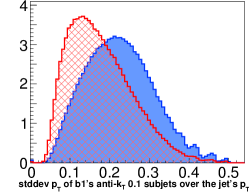
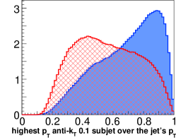
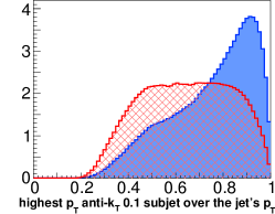
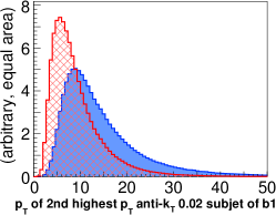
Figure 8: Some subjet variable distributions for $ZH$ signal (solid blue) and $Zb\bar{b}$ background (hashed red) athe LHC. Events satisfy selection cuts and the Higgs mass-window cut, $90\,\mathrm{GeV}<{m_{b\bar{b}}}<124\,\mathrm{GeV}$. Horizontal axes are in radians or GeV as appropriate, and vertical axes are in arbitrary units with signal and background normalized to the same area.

3.6 Radial Moments: Girth and Jet Angularities

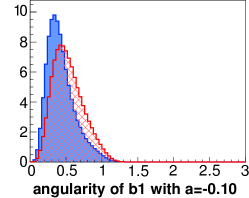
Figure 9: Girth and angularity distributions for $ZH$ signal (solid blue) and $Z{b\bar{b}}$ background (hashed red) at the LHC. Events satisfy selection cuts and the Higgs mass-window cut, $90\,\mathrm{GeV}<{m_{b\bar{b}}}<124\,\mathrm{GeV}$. Horizontal axes are in radians or GeV as appropriate, and vertical axes are in arbitrary units with signal and background normalized to the same area.

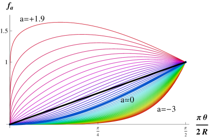
Figure 10: Profiles for different choices of the angularity $a$ parameter spaced at 0.1 intervals (in rainbow) and linear radial-moment “girth” (in black)

The distribution of particles within a jet can be can be useful for distinguishing jets initiated by different flavors of quark or by a gluon. Even in our signal and irreducible background with two $b$-tagged jets, this distribution has proven useful.

One infrared safe way of characterizing the jets is to integrate (sum) the energy or $p_{T}$ distribution against a radially symmetric profile. Different choices of profile and overall normalization lead to different observables. Distances $r_{i}$ of each particle or cell are calculated in $(y,\phi)$ space with respect the location of the jet. The jet location $(y,\phi)$ is defined by the anti-$k_{T}$ algorithm ‘E-scheme’ as the 4-vector sum of all inputs (particles or calorimeter towers.) It is important to use rapidity (rather than pseudorapidity) for the jet location because the jet is massive in this scheme. A radial moment sums these distances (or a function of these distances), weighted by a quantity like $p_{T}$, then normalized to the total $p_{T}$ of the jet. For example, the linear radial moment, girth, is defined as [9]

$$\textrm{Girth}:\qquad g=\sum_{i\in\mathrm{jet}}\frac{p_{T}^{i}\,|r_{i}|}{p_{T}^{jet}}\,.$$ (5)

The girth distribution is shown in Figure 9.

Jet Angularities are also radial moments, but their “radial distances” are rescaled into the angular coordinates appropriate for $e^{+}e^{-}$ event shapes. They are defined by [20]

$$\textrm{Jet Angularities}:~{}~{}~{}~{}A_{a}=\frac{1}{m_{jet}}\sum_{i\in\mathrm{jet}}E_{i}\ f_{a}(\frac{\pi|r_{i}|}{2R})\,,$$ (6)

with

$$f_{a}(\theta)=\sin^{a}\!\theta\,\left(1-\cos\theta\right)^{1-a}\,,$$ (7)

with $a<2$. The kernel function $f_{a}(\theta)$ is inspired by full event-shape angularities [21], but modified so that the edge of a jet at $|r_{i}|\!=\!R$ is mapped to $\pi/2$. Profiles for different choices of the $a$ parameter are shown in Figure 10. Note that the energies $E_{i}$ are used in the definition, instead of $p_{T}$’s, and the angularities are normalized by the jet mass. Radial moments like jet angularities and girth are especially interesting because it may be possible to calculate them accurately in QCD, see for example [22].

3.7 Pull

Pull tries to capture the difference in color structure between the Higgs boson signal and the QCD background. It was introduced in Ref. [9], and then immediately used in the DØ search [23] for $ZH$ with $Z\to\nu\bar{\nu}$.

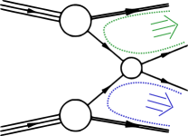
Figure 11: Color connections for a signal-like ($pp\to H\to{b\bar{b}}$) on the left and background-like ($pp\to{b\bar{b}}$) on the right. Our signal and background each have a colorless $Z$ or $W$ (not shown) radiating from of one of the hard quark lines and decaying to leptons. This doesn’t affect the color flow.

To leading order in the number of colors (up to $1/N_{\text{colors}}^{2}\sim 10\%$ corrections), quarks can be described as being “color-connected” to other quarks by a “color string” Ref. [10]. This approximation governs much of the parton shower. The color-singlet Higgs boson decays to two $b$-quarks that are color-connected to each other, while $b$’s from the background are color-connected to the proton remnants that travel down the beam pipe. This is shown schematically in Figure 11. This difference is independent of the event kinematics, and therefore, if observable, should be be complementary to kinematical variables and useful in a multi-variable search.

The pull vector is designed to measure color flow. It is a $p_{T}$ weighted moment vector that tends to point toward the color-connected partner of the jet’s initiating quark. The pull vector is defined as

$$\textrm{Pull Vector }\vec{t}=\sum_{i\in\mathrm{jet}}\frac{p_{T}^{i}\,|r_{i}|}{p_{T}^{jet}}\,\vec{r}_{i}\qquad\textrm{where }\vec{r}_{i}\equiv(y_{i}-y_{\mathrm{jet}},\phi_{i}-\phi_{\mathrm{jet}})\,.$$ (8)

Without the factor of $|r_{i}|$, this would be the jet’s $p_{T}$-weighted centroid. For fixed kinematics, pull has been shown to help separate signal from background [9]. For example, if we fix the $b$’s to have $(\Delta\eta,\Delta\phi)=(1,2)$ with $p_{T}^{H}=200$ GeV, the average $p_{T}$ measured in the calorimeter is shown for signal and background in Figure 12. The difference in $p_{T}$ distributions around the jets holds up even for individual events. The most effective way to use the pull vector is to calculate a pull angle, which is the angle between the pull vector and some other vector in the event. We will now point out some technical details that help make pull more effective, and define some example pull angles, such as the ones drawn in Figure 12 which are defined in Table 3.

Signal Accumulated $\mathbf{p_{t}}$	Background Accumulated $\mathbf{p_{t}}$
\psfrag{th}{$\theta_{p}$}\psfrag{mp}{$\left|\vec{p}\right|$}\psfrag{mpi}{\scriptsize$-\pi$}\psfrag{pi}{\scriptsize$\pi$}\psfrag{0.04}{\scriptsize$0.04$}\psfrag{0.02}{\scriptsize$0.02$}\psfrag{0}{\scriptsize$0$}\includegraphics[width=195.12767pt]{accHZ}	\psfrag{th}{$\theta_{p}$}\psfrag{mp}{$\left|\vec{p}\right|$}\psfrag{mpi}{\scriptsize$-\pi$}\psfrag{pi}{\scriptsize$\pi$}\psfrag{0.04}{\scriptsize$0.04$}\psfrag{0.02}{\scriptsize$0.02$}\psfrag{0}{\scriptsize$0$}\includegraphics[width=195.12767pt]{accZbb}

Figure 12: A single parton-level signal event showered millions of times (left) and a single parton-level background event with identical kinematics but different color connections showered millions of times (right). The color shows the average showered $p_{T}$ density in $(\eta,\phi)$ for an ensemble of events with fixed parton-level kinematics. (Contours are stepped in factors of two.) Results for $ZH\to Z{b\bar{b}}$ are displayed on the left, and $gg\to Z{b\bar{b}}$ on the right. The underlying color connections are shown with thin lines, and examples of pull vectors (which would be defined event-by-event) with arrows. The angles $\alpha_{1,2}$ and $\beta_{1,2}$ are illustrated as the angles of the pull vectors with respect to the “signal-like” and “background-like” color connection lines.

Signal xxxx pull angles	$\alpha_{1}=$ angle between the high-$p_{T}$ jet’s pull and the direction to the low $p_{T}$ jet	$\alpha_{2}=$ angle between the low-$p_{T}$ jet’s pull and the direction to the high $p_{T}$ jet	Signal xxxx pull distance x $\alpha=\sqrt{\alpha_{1}^{2}+\alpha_{2}^{2}}$
Background pull angles	$\beta_{1}=$ angle between the high-$p_{T}$ jet’s pull and the direction to nearest beam	$\beta_{2}=$ angle between the high-$p_{T}$ jet’s pull and the direction to nearest beam	Background pull distance x $\beta=\sqrt{\beta_{1}^{2}+\beta_{2}^{2}}$

Table 3: Definition of useful pull angles..

We found it important to use anti-$k_{T}$ jets because the highest energy jets in the event tend to be circular, whereas the split-merge procedure of a cone-jet algorithm can nibble away pieces and combine them with an adjacent jet. If that adjacent jet came from a perturbative QCD radiation (due to the color-connection in the dipole picture), these are exactly the pieces that should be contributing most to the pull. It’s also important that real rapidity $y$ be used, as opposed to pseudo-rapidity $\eta$. While this is less important for each calorimeter cell, the 4-momenta of a jet can be massive when constructed by adding together massless calorimeter 4-momenta (the “E-Scheme”). If anti-$k_{T}$ jets are not available, the next best option is to use a circular area in the $y/\phi$ plane around the jet’s $y/\phi$ centroid.

\psfrag{pull_toward_otherjet_b_highPt__1_Pt_4v_y}{\tiny{pull of high-$p_{T}$ $b$ jet: $\alpha_{1}$}}\psfrag{pull_toward_otherjet_b_lowPt__1_Pt_4v_y}{\tiny{pull of low-$p_{T}$ $b$ jet: $\alpha_{2}$}}\psfrag{pull_dist_between_otherjet_b_highPt__1_Pt_4v_y}{\tiny{pull signal-distance: $\alpha$}}\psfrag{pull_uncrosssed_b_highPt__1_Pt_4v_y}{\tiny{pull of high-$p_{T}$ $b$ jet: $\beta_{1}$}}\psfrag{pull_uncrosssed_b_lowPt__1_Pt_4v_y}{\tiny{pull of low-$p_{T}$ $b$ jet: $\beta_{2}$}}\psfrag{pull_dist_uncrosssed_otherjet_b_highPt__1_Pt_4v_y}{\tiny{pull backgnd-distance: $\beta$}}\includegraphics[width=130.08731pt]{rainbows/pull_toward_otherjet_b_highPt_ak05_1_Pt_4v_y}

\psfrag{pull_toward_otherjet_b_highPt__1_Pt_4v_y}{\tiny{pull of high-$p_{T}$ $b$ jet: $\alpha_{1}$}}\psfrag{pull_toward_otherjet_b_lowPt__1_Pt_4v_y}{\tiny{pull of low-$p_{T}$ $b$ jet: $\alpha_{2}$}}\psfrag{pull_dist_between_otherjet_b_highPt__1_Pt_4v_y}{\tiny{pull signal-distance: $\alpha$}}\psfrag{pull_uncrosssed_b_highPt__1_Pt_4v_y}{\tiny{pull of high-$p_{T}$ $b$ jet: $\beta_{1}$}}\psfrag{pull_uncrosssed_b_lowPt__1_Pt_4v_y}{\tiny{pull of low-$p_{T}$ $b$ jet: $\beta_{2}$}}\psfrag{pull_dist_uncrosssed_otherjet_b_highPt__1_Pt_4v_y}{\tiny{pull backgnd-distance: $\beta$}}\includegraphics[width=130.08731pt]{rainbows/pull_toward_otherjet_b_lowPt_ak05_1_Pt_4v_y}

\psfrag{pull_toward_otherjet_b_highPt__1_Pt_4v_y}{\tiny{pull of high-$p_{T}$ $b$ jet: $\alpha_{1}$}}\psfrag{pull_toward_otherjet_b_lowPt__1_Pt_4v_y}{\tiny{pull of low-$p_{T}$ $b$ jet: $\alpha_{2}$}}\psfrag{pull_dist_between_otherjet_b_highPt__1_Pt_4v_y}{\tiny{pull signal-distance: $\alpha$}}\psfrag{pull_uncrosssed_b_highPt__1_Pt_4v_y}{\tiny{pull of high-$p_{T}$ $b$ jet: $\beta_{1}$}}\psfrag{pull_uncrosssed_b_lowPt__1_Pt_4v_y}{\tiny{pull of low-$p_{T}$ $b$ jet: $\beta_{2}$}}\psfrag{pull_dist_uncrosssed_otherjet_b_highPt__1_Pt_4v_y}{\tiny{pull backgnd-distance: $\beta$}}\includegraphics[width=130.08731pt]{rainbows/pull_dist_between_otherjet_b_highPt_ak05_1_Pt_4v_y}

\psfrag{pull_toward_otherjet_b_highPt__1_Pt_4v_y}{\tiny{pull of high-$p_{T}$ $b$ jet: $\alpha_{1}$}}\psfrag{pull_toward_otherjet_b_lowPt__1_Pt_4v_y}{\tiny{pull of low-$p_{T}$ $b$ jet: $\alpha_{2}$}}\psfrag{pull_dist_between_otherjet_b_highPt__1_Pt_4v_y}{\tiny{pull signal-distance: $\alpha$}}\psfrag{pull_uncrosssed_b_highPt__1_Pt_4v_y}{\tiny{pull of high-$p_{T}$ $b$ jet: $\beta_{1}$}}\psfrag{pull_uncrosssed_b_lowPt__1_Pt_4v_y}{\tiny{pull of low-$p_{T}$ $b$ jet: $\beta_{2}$}}\psfrag{pull_dist_uncrosssed_otherjet_b_highPt__1_Pt_4v_y}{\tiny{pull backgnd-distance: $\beta$}}\includegraphics[width=130.08731pt]{rainbows/pull_uncrosssed_b_highPt_ak05_1_Pt_4v_y}

\psfrag{pull_toward_otherjet_b_highPt__1_Pt_4v_y}{\tiny{pull of high-$p_{T}$ $b$ jet: $\alpha_{1}$}}\psfrag{pull_toward_otherjet_b_lowPt__1_Pt_4v_y}{\tiny{pull of low-$p_{T}$ $b$ jet: $\alpha_{2}$}}\psfrag{pull_dist_between_otherjet_b_highPt__1_Pt_4v_y}{\tiny{pull signal-distance: $\alpha$}}\psfrag{pull_uncrosssed_b_highPt__1_Pt_4v_y}{\tiny{pull of high-$p_{T}$ $b$ jet: $\beta_{1}$}}\psfrag{pull_uncrosssed_b_lowPt__1_Pt_4v_y}{\tiny{pull of low-$p_{T}$ $b$ jet: $\beta_{2}$}}\psfrag{pull_dist_uncrosssed_otherjet_b_highPt__1_Pt_4v_y}{\tiny{pull backgnd-distance: $\beta$}}\includegraphics[width=130.08731pt]{rainbows/pull_uncrosssed_b_lowPt_ak05_1_Pt_4v_y}

\psfrag{pull_toward_otherjet_b_highPt__1_Pt_4v_y}{\tiny{pull of high-$p_{T}$ $b$ jet: $\alpha_{1}$}}\psfrag{pull_toward_otherjet_b_lowPt__1_Pt_4v_y}{\tiny{pull of low-$p_{T}$ $b$ jet: $\alpha_{2}$}}\psfrag{pull_dist_between_otherjet_b_highPt__1_Pt_4v_y}{\tiny{pull signal-distance: $\alpha$}}\psfrag{pull_uncrosssed_b_highPt__1_Pt_4v_y}{\tiny{pull of high-$p_{T}$ $b$ jet: $\beta_{1}$}}\psfrag{pull_uncrosssed_b_lowPt__1_Pt_4v_y}{\tiny{pull of low-$p_{T}$ $b$ jet: $\beta_{2}$}}\psfrag{pull_dist_uncrosssed_otherjet_b_highPt__1_Pt_4v_y}{\tiny{pull backgnd-distance: $\beta$}}\includegraphics[width=130.08731pt]{rainbows/pull_dist_uncrosssed_otherjet_b_highPt_ak05_1_Pt_4v_y}

Figure 13: Pull distributions for $ZH$ signal (solid blue) and $Zb\bar{b}$ background (hashed red) at the LHC. Events satisfy selection cuts and the Higgs mass-window cut, $90\,\mathrm{GeV}<{m_{b\bar{b}}}<124\,\mathrm{GeV}$. Horizontal axes are in radians, and vertical axes are in arbitrary units with signal and background normalized to the same area.

The 2D distribution of the $y$ and $\phi$ components of the pull vector looks like a Gaussian whose peak is shifted slightly away from the origin in the direction of the color-connected object. The magnitude of the vector does not have as much distinguishing power as its angle. The pull angle of each jet, however, does not have much power without comparing it to where it “should” point: toward the other jet for the signal, and toward one of the beams (usually the closest) for the background.

The direction toward the other $b$-jet is the twist angle, defined in Section 3.2. A version of twist that goes from 0 to $2\pi$ is defined as the direction of the lower-$p_{T}$ jet from the location of the higher-$p_{T}$ jet in the $y/\phi$ plane. The 3D distribution of the pull angles of each jet along with this twist angle contains all of the useful pull information that can be used to separate signal from background, but the individual pull angles for a given event are meaningful only with respect to the twist angle. In an attempt to expose the physics and make the job of a multivariate discriminator easier, we begin by defining four variables that more directly capture where the pulls “should” point for the signal and background, labeled in Figure 12 and defined Table 3.

Subtracting the pull vectors is not useful, since the magnitude of each vector does not carry much meaning, and the magnitudes are independent of each other. Many other attempts to combine the pull angles into a single variable also sacrifice discrimination power. The best we have achieved is the “pull distance,” the square root of the sum of squares of the difference angles. These pull angles are defined in Table 3.

3.8 Total Energy Variables

Next, we consider general purpose variables which look at the event as a whole. Examples include

• $\hat{s}$ = CM energy for hard collision, or invariant mass of the reconstructed Higgs boson and Z.

• $H_{T}$ = Scalar sum of all $E_{T}$.

• $H_{z}$ = Boost of the center-of-mass system along the beam.

• $\Sigma p_{T}$ = Scalar sum of all $p_{T}$ (which differs from $H_{T}$ for massive jets).

• $E_{vis}$ = Scalar sum of all visible energy.

• Centrality $=\Sigma p_{T}\ /\ E_{vis}$.

For each of these variables, the quantity can be constructed from the complete event, summing over all particles in the event. Particles here can mean topo-clusters or calorimeter cells or energy deposits coarse-grained into $0.1\times 0.1$ cells in $(\eta,\phi)$. In this study we use the 4-momenta of the stable particles in the event record for what we call the particle variables. The same variables can also be constructed using just the reconstructed objects (jets, leptons and photons) or even just the four primary objects (2 $b$-jets and 2 leptons). We find that using objects generally works much better than using variables constructed from energy in the complete event. A particularly useful variable is centrality constructed from the four primary objects. Some energy variables are shown in Figure 14.

3.9 Event Shape Variables

Finally, we look at some event shape variables. The ones we consider involve eigenvalues of two similar tensors composed of 3-momenta, with the sum over the same sets of particles, reconstructed objects, or four primary objects, as above:

$$\begin{array}[]{lll}\textrm{Sphericity Tensor }\equiv&&\textrm{Spherocity Tensor }\equiv\\ \dfrac{1}{\Sigma_{i}|\vec{p}_{i}|^{2}}\sum_{i}\begin{pmatrix}p_{x}p_{x}&p_{x}p_{y}&p_{x}p_{z}\\ p_{y}p_{x}&p_{y}p_{y}&p_{y}p_{z}\\ p_{z}p_{x}&p_{z}p_{y}&p_{z}p_{z}\end{pmatrix}&&\dfrac{1}{\Sigma_{i}|\vec{p}_{i}|}\sum_{i}\left[\dfrac{1}{|\vec{p}_{i}|}\begin{pmatrix}p_{x}p_{x}&p_{x}p_{y}&p_{x}p_{z}\\ p_{y}p_{x}&p_{y}p_{y}&p_{y}p_{z}\\ p_{z}p_{x}&p_{z}p_{y}&p_{z}p_{z}\end{pmatrix}\right]\\ \end{array}$$ (9)

where $i$ labels on the momentum components appearing in the matrix are implicit.

The eigenvalues of these matrices are computed, then ordered and normalized $\lambda_{1}\geq\lambda_{2}\geq\lambda_{3}$ with $\lambda_{1}+\lambda_{2}+\lambda_{3}=1$. The event shapes are then defined as [24]

• Sphericity and Spherocity: $S=\frac{3}{2}\,(\lambda_{2}+\lambda_{3})$ where $0\leq S\leq 1$. A 2-jet event has $S\approx 0$ while an isotropic one has $S\approx 1$.

• Aplanarity and Aplanority: $A=\frac{3}{2}\,\lambda_{3}$ where $0\leq A\leq 1/2$. A planar event has $A\approx 0$ while an isotropic one has $A\approx 1/2$.

• Y variable from Sphericity: $Y=\frac{\sqrt{3}}{2}\,(\lambda_{2}-\lambda_{3})$.

• DShape from Spherocity: $D=27\,\lambda_{1}\lambda_{2}\lambda_{3}$.

Sphericity, Spherocity, and DShape are all highly correlated, Aplanarity and Aplanority are too, as are the shapes derived from the four primary objects in the lab and CM frame. Aplanarity seems to be the most useful shape variables. The others seem useful only to the extent they are correlated with Aplanarity or Centrality. Some event shapes are shown in Figure 14. We also consider the Fox-Wolfram moments of particles, objects, and primary objects. These are defined by projecting against the Legendre polynomials

$$H_{\ell}=\frac{1}{E_{vis}}\Sigma_{i,j}|p_{i}||p_{j}|P_{\ell}(\cos\theta_{ij})\,.$$ (10)

The Fox-Wolfram moments were not found particularly useful.

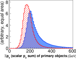
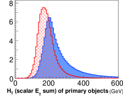
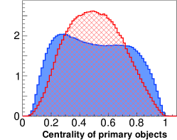
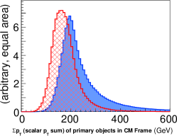
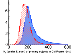
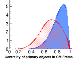
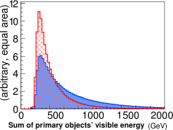
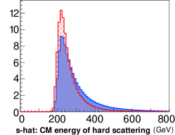
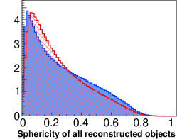
Figure 14: Total energy and event shape variables for $ZH$ signal (solid blue) and $Zb\bar{b}$ background (hashed red) at the LHC. Events satisfy selection cuts and the Higgs mass-window cut, $90\,\mathrm{GeV}<{m_{b\bar{b}}}<124\,\mathrm{GeV}$. Horizontal axes are in GeV where appropriate, and vertical axes are in arbitrary units with signal and background normalized to the same area.

3.10 Missing $E_{T}$ variables

Missing $E_{T}$ and missing $p_{T}$ are not included in this analysis, other than the neutrino used to reconstruct the $W$ in the $WH$ channel. From an experimental point of view, missing $E_{T}$ is an extremely important variable. However, its distribution is dominated strongly by experimental mis-measurements and calorimeter resolution. Without a full detector simulation, missing energy is inappropriate for our particle-level study and, in fact, causes unphysical instabilities if included in the multi-variable analysis.

4 Efficiency measures

Having cataloged our input variables, we can now explore which ones have the best distinguishing power. For single variables, we look at the effect that a simple cut or window (two-sided cut) has on the number of signal and background events in our fiducial ${m_{b\bar{b}}}$ window. To combine variables, we will use more sophisticated methods, described in the next section. But for single variables, cuts are as good as one can do.

Any given cut will keep some fraction $\varepsilon_{S}$ of signal events and some other fraction $\varepsilon_{B}$ of background events. These are the signal and background efficiencies of the cut. For the two sided cuts, there are a number of choices which give the same $\varepsilon_{S}$, so the one which minimizes $\varepsilon_{B}$ for a given $\varepsilon_{S}$ is chosen. A standard way to visualize the relationship between $\varepsilon_{S}$ and $\varepsilon_{B}$ is with a “Receiver Operating Characteristic” curve, or ROC curve. Often the background rejection $1-\varepsilon_{B}$, or the inverse rejection $\frac{1}{\varepsilon_{B}}$ is plotted against the signal efficiency $\varepsilon_{S}$. A sample ROC curve for 10 representative single variables is shown in Figure 15. Lower lines are better, since they give more background rejection for the same signal efficiency, but since some of the curves cross, the ROC curves do not lead to an immediate observation of which variables are better. One approach to ranking variables would be to arbitrarily demand a particular signal efficiency and find the variables that give the best background rejection, but we propose a more useful procedure that does not introduce an arbitrary parameter.

\psfrag{LHC HZ Signal and Background Efficiencies}{LHC ZH \qquad ROC Curve : $\varepsilon_{B}$ vs $\varepsilon_{S}$}\psfrag{LHC ZH : Significance : }{}\psfrag{Signal eff}{\!\!\!\!\!\!\!\!\!\!\!\!\!\!\!\!\!\!\!\!\!\!\!\!\!\!\!\!\!\!\!\!\!\!\!\!\!\!\!\!\!\!\!\!\!\!\! \footnotesize{Higgs Signal Efficiency $\varepsilon_{S}$}}\psfrag{Backgr eff}{\!\!\!\!\!\!\!\!\!\!\!\!\!\!\!\!\!\!\!\!\!\!\!\!\!\!\!\!\!\!\!\!\!\!\!\!\!\!\!\!\!\!\!\!\!\!\!\!\!\!\!\!\!\!\!\!\!\!\!\!\! \footnotesize{Background Efficiency $\varepsilon_{B}$}}\psfrag{b_highPt_Pt_ak05}{\scriptsize{$p_{T}^{b1}$}}\psfrag{b_lowPt_Pt_ak05}{\scriptsize{$p_{T}^{b2}$}}\psfrag{Z_Pt_ak05}{\scriptsize{$p_{T}^{Z}$}}\psfrag{bbbar_twist_ak05}{\scriptsize{$\tau_{b\bar{b}}$}}\psfrag{bbbar_dEta_ak05}{\scriptsize{$\Delta\eta_{b\bar{b}}$}}\psfrag{H_and_b_lowPt_dRap_ak05}{\scriptsize{$\Delta y_{H,b2}$}}\psfrag{H_and_b_highPt_dRap_ak05}{\scriptsize{$\Delta y_{H,b1}$}}\psfrag{ZZH_Frame_b_lowPt_costheta_ak05}{\scriptsize{CM $\cos(\theta_{b2})$}}\psfrag{bbbar_dR_ak05}{\scriptsize{$\Delta R_{b\bar{b}}$}}\psfrag{lplm_dPhi_ak05}{\scriptsize{$\Delta\phi_{\ell^{+}\ell^{-}}$}}\includegraphics[width=303.53267pt]{analHZmarg56alt_Likelihood_ak05_kinematic_ROCs_mod}

Figure 15: ROC curves for some variables, showing the background efficiency and signal efficiency as parametric functions of the cut value.

In order to quantify the usefulness of a variable, we need to consider the goal of the signal search. The signal-to-background ratio ($S/B$) and the significance ($\sigma\sim S/\sqrt{B}$) are the two quantities considered when trying to see a signal over a large background. Making a tighter cut will reduce both efficiencies, but not necessarily by the same amount, so $S/B$ may change. The factor by which $S/B$ changes is just the ratio of the efficiencies.

$$\frac{S}{B}\qquad\stackrel{{\scriptstyle\scriptscriptstyle\text{cut}}}{{\rightarrow}}\qquad\frac{\varepsilon_{S}S}{\varepsilon_{S}B}=\left(\frac{\varepsilon_{S}}{\varepsilon_{B}}\right)\frac{S}{B}\,.$$ (11)

The other quantity normally considered is the statistical significance $\sigma$ which, for large numbers of events, approaches $S/\sqrt{B}$. For a convincing discovery, the expected number of signal events must exceed the statistical fluctuations of the background:

$$\frac{S}{\sqrt{B}}\gg 1\,.$$ (12)

When we cut on our discriminant, the significance changes by

$$\sigma\equiv\frac{S}{\sqrt{B}}\qquad\stackrel{{\scriptstyle\scriptscriptstyle\text{cut}}}{{\rightarrow}}\qquad\frac{\varepsilon_{S}S}{\sqrt{\varepsilon_{B}B}}=\left(\frac{\varepsilon_{S}}{\sqrt{\varepsilon_{B}}}\right)\sigma\,.$$ (13)

It follows that the two quantities we are interested in are the signal-over-background improvement characteristic

$$\frac{\varepsilon_{S}}{\varepsilon_{B}}\,,$$ (14)

and the Significance Improvement Characteristic (SIC)

$${\text{\sc SIC}}\equiv\frac{\varepsilon_{S}}{\sqrt{\varepsilon_{B}}}\,.$$ (15)

These quantities tell us the improvement on $S/B$ and $\sigma$ that our discriminant will give. When systematics dominate, $\varepsilon_{S}/\varepsilon_{B}$ is more important, and when statistical errors dominate, SIC is the more useful measure. Given that $\varepsilon_{S}/\varepsilon_{B}$ and SIC are luminosity independent, they provide good measures of the relative discrimination power of the various variables. Moreover, plotting these measures, especially SIC as functions of $\varepsilon_{S}$ provides a wonderful visualization of a variable’s effectiveness.

\psfrag{LHC HZ Signal over Background}{~{}~{}~{}~{}\tiny{$\text{LHC ZH Signal over Background}$}}\psfrag{Signal eff}{\!\!\!\!\!\!\!\!\!\!\!\!\!\!\!\!\!\!\!\!\!\!\!\!\!\!\!\!\!\!\!\!\!\!\!\!\!\!\!\!\!\!\!\!\!\!\!\tiny{Higgs Signal Efficiency $\varepsilon_{S}$}}\psfrag{b_highPt_Pt_ak05}{\tiny{$p_{T}^{b1}$}}\psfrag{b_lowPt_Pt_ak05}{\tiny{$p_{T}^{b2}$}}\psfrag{Z_Pt_ak05}{\tiny{$p_{T}^{Z}$}}\psfrag{bbbar_twist_ak05}{\tiny{$\tau_{b\bar{b}}$}}\psfrag{bbbar_dEta_ak05}{\tiny{$\Delta\eta_{b\bar{b}}$}}\psfrag{H_and_b_lowPt_dRap_ak05}{\tiny{$\Delta y_{H,b2}$}}\psfrag{H_and_b_highPt_dRap_ak05}{\tiny{$\Delta y_{H,b1}$}}\psfrag{ZZH_Frame_b_lowPt_costheta_ak05}{\tiny{CM $\cos(\theta_{b2})$}}\psfrag{bbbar_dR_ak05}{\tiny{$\Delta R_{b\bar{b}}$}}\psfrag{lplm_dPhi_ak05}{\tiny{$\Delta\phi_{\ell^{+}\ell^{-}}$}}\includegraphics[width=216.81pt]{analHZmarg56alt_Likelihood_ak05_kinematic_ROCsSoverB_mod}

\psfrag{LHC HZ Significance}{\tiny{$S/\sqrt{B}$ Improvement}}\psfrag{Signal eff}{\!\!\!\!\!\!\!\!\!\!\!\!\!\!\!\!\!\!\!\!\!\!\!\!\!\!\!\!\!\!\!\!\!\!\!\!\!\!\!\!\!\!\!\!\!\!\!\tiny{Higgs Signal Efficiency $\varepsilon_{S}$}}\psfrag{b_highPt_Pt_ak05}{\tiny{$p_{T}^{b1}$}}\psfrag{b_lowPt_Pt_ak05}{\tiny{$p_{T}^{b2}$}}\psfrag{Z_Pt_ak05}{\tiny{$p_{T}^{Z}$}}\psfrag{bbbar_twist_ak05}{\tiny{$\tau_{b\bar{b}}$}}\psfrag{bbbar_dEta_ak05}{\tiny{$\Delta\eta_{b\bar{b}}$}}\psfrag{H_and_b_lowPt_dRap_ak05}{\tiny{$\Delta y_{H,b2}$}}\psfrag{H_and_b_highPt_dRap_ak05}{\tiny{$\Delta y_{H,b1}$}}\psfrag{ZZH_Frame_b_lowPt_costheta_ak05}{\tiny{CM $\cos(\theta_{b2})$}}\psfrag{bbbar_dR_ak05}{\tiny{$\Delta R_{b\bar{b}}$}}\psfrag{lplm_dPhi_ak05}{\tiny{$\Delta\phi_{\ell^{+}\ell^{-}}$}}\includegraphics[width=216.81pt]{analHZmarg56alt_Likelihood_ak05_kinematic_ROCsSignif_mod}

Figure 16: Improvements in $S/B$ and $\sigma=S/\sqrt{B}$ for the same variables as in the previous figure.

We show $\varepsilon_{S}/\varepsilon_{B}$ and SIC as a function of $\varepsilon_{S}$ in Figure 16 for the same 10 variables as in the ROC curve in Figure 15. There are a few salient features of these more powerful visualizations. First, consider the $S/B$ curves. There are apparently two classes of variables. For one class (including $\Delta\eta_{b\bar{b}}$ and other angle-type variables), the $S/B$ is essentially flat below $\varepsilon_{S}\sim 0.7$ or so. This means that the variable cannot distinguish signal from background beyond this point, and cutting harder on these variable is equivalent to throwing out random events. The other class (including $p_{T}^{Z}$ and other variables with long tails) seem to lead to $S/B$ enhancements which grow indefinitely towards $\varepsilon_{S}=0$. This means that if sufficiently hard cuts are placed, a very large improvement in $S/B$ can be achieved. This often happens because there is some limit of the variable in which there are zero background events. These qualitative observations notwithstanding, it is not at all clear, by looking at the $\varepsilon_{S}/\varepsilon_{B}$ curves alone, which variable does best, or where to apply the cut. For this reason, we will focus less on these curves for the multivariate analysis than on SIC.

The SIC curves provide a much better way of looking at the information than the $\varepsilon_{S}/\varepsilon_{B}$ curves. We see that there are still essentially two classes. For one class (including $\Delta\eta_{b\bar{b}}$), the efficiencies have a maximum at some intermediate value of $\varepsilon_{S}$. Thus, there is an optimal value of the cut for these variables to get the maximal enhancement in $S/\sqrt{B}$. Because of this maximum, we argue that

$$\overline{\text{\sc SIC}}\equiv\max\frac{\varepsilon_{S}}{\sqrt{\varepsilon_{B}}}$$ (16)

is a useful characterization of the effectiveness of a discrimination method. The other class of variables (including $p_{T}^{Z}$) seem to only be able to reduce $S/\sqrt{B}$ and have $\overline{\text{\sc SIC}}=1$.

The variables which can lead to $S/\sqrt{B}$ improvement are often ones which had flat $S/B$ distributions. Also, the variables which lead to arbitrarily large $S/B$ enhancements often can only reduce $S/\sqrt{B}$. Since $p_{T}^{Z}$ is one of the second class of variables, the original efficiencies from the boosted Higgs boson search [5] were $\varepsilon_{S}=1/20$ and $\varepsilon_{B}=1/320$. We see that $\varepsilon_{S}/\varepsilon_{B}=16$ while $\varepsilon_{S}/\sqrt{\varepsilon_{B}}=0.89$.

Starting from these observations, we turn to the multivariate analysis. Among other things, we will find that some variables which are useless as single variables (i.e. $\overline{\text{\sc SIC}}=1$) start to add marginal efficiency on top of the ones which are useful to begin with. Moreover, we will see that the optimal set of 10 variables is very different from the top 10 single variables. This makes perfect sense: less useful variables can become useful after cuts on more powerful variables are applied, because they have subtle correlations. However, this means we have to carefully decide on which variables to use, in order avoid throwing out some potentially useful ones which are not useful by themselves. A systematic procedure for selecting a set of variables is described in Section 6. First, we give a brief introduction to the multivariate methods.

5 Multivariate Techniques 

In order to make use of all possible discriminating features between signal and background samples, including complex non-linear correlations, we will make use of a multivariate approach. Many multivariate techniques are efficiently implemented in the Toolkit for Multivariate Data Analysis with ROOT (TMVA) in a way that makes them easy to use and compare. We refer the reader to the TMVA documentation for more details of the methods [16].

In this study, we will use mainly Boosted Decision Trees (BDTs) [25]. We briefly considered other methods, such as multilayer perceptron Artificial Neural Networks (ANNs). We found that BDTs tend to converge faster and run in shorter time than ANN while giving similar results. We suspect that ANNs may be optimal for other applications, such as artificial intelligence, but for high energy physics analyses, they are not entirely appropriate. The main feature that distinguishes the particle physics applications is that we are almost always interested in a binary classification: signal vs background. Neural networks seem better suited for multidimensional outputs, such as in pattern recognition tasks. (For a more detailed comparison in the context of a particle physics application, with similar conclusions, see [26, 27].) We also found that a traditional Bayesian likelihood analysis or optimal linear Fisher discriminant is comparable to the BDT for few variables, but does significantly worse when multiple variables are combined. Performing a thorough comparison of methods in the context of collider physics is beyond the scope of the current study. The results in this paper will all refer to discrimination using the BDT method, which we found optimal in our informal survey of different methods and different parameters.

A decision tree is a hierarchical set of one-sided cuts used to classify signal (S) versus background (B). For example, if there are two discriminants $a$ and $b$, a tree might be: if $a>2$ then $\{$if $b<4$ then S$\}$ else $\{$if $b>5$ then S$\}$ else B. One can, in principle, find the single best tree for discriminating S from B within a given Monte Carlo sample of training events, and given certain constraints on how many cuts we are allowed to apply. Once this tree is found, one can then attempt to train another tree to classify correctly the events that the first tree misclassified (i.e. background events that end up in regions designated as “signal-like” by the tree, and vice-versa). Then one can train a third tree to attempt to correct misclassifications of the second tree, and so on. Typically, this is repeated until a “forest” of $O(1000)$ trees has been constructed. Each successive tree is trained on the same Monte Carlo sample, but at each stage a boost is applied: misclassified events from the previous tree are increased in weight, so that the next tree will work harder to better classify them. After building up the forest, a weighted vote is taken between all of the trees to form the final discriminant at each point in the multivariate phase space. By varying a cut on the weighted vote, i.e. asking that at least $x\%$ of the trees classify an event as signal for it to pass, the BDT provides a nearly continuous efficiency measure parametrized by $x$. Thus, varying $x$ can generate the ROC and SIC curves for our analysis.

For a single variable, a single tree is sufficient. If the variable is monotonic in signal and background, a one-sided cut can be proven optimal. If the distributions rise and then fall, a two-sided cut is optimal. For more than one variable, the optimal solution can be calculated exactly, using a Bayesian likelihood. However, to use the Bayesian approach one needs to know the distributions essentially analytically. This is impossible when many variables are involved, and one can only sample phase space. In this case, the best one can do is to know the differential cross sections for events in the vicinity of the candidate event’s kinematics. For such large under-sampled phase space, the Bayesian likelihood approach is inefficient and multivariate techniques like BDTs are needed.

As an example, consider the signal and background distributions for the two variables $\Delta\theta_{b1,\ell 1}$ and $\Delta\eta_{b2,\ell 1}$, as shown in Figure 17. These two variables are chosen simply because they have unusual correlations. With our large event samples, we can produce an essentially smooth 2-dimensional distribution in these variables. Each axis in these figures is sampled into 50 divisions, leading to 2500 bins. From these distributions, we compute the “exact” 2D probability density, as shown in the third panel of this figure. For two variables, the phase space is sampled finely enough that this full likelihood discriminant is computable. Next, we ask how well a BDT classifier can reproduce this likelihood distribution. In Figure 18, we present the result of a BDT using 2, 8 and 256 trees trained on the same 2-dimensional data set. Even with their rectangular cuts, we see that the BDTs do a good job characterizing the correlations of the the full 2D probability density. Certainly 8 and even 256 trees require many fewer events to train than are needed to sufficiently populate the 2500 bins of the sampled likelihood. For higher dimensional phase space, we find that a reasonable number of trees continues to sample the space well, while a uniform sampling required for a likelihood approach is impossible. We use up to 3000 trees for 10 variables, although our results barely change beyond 400 trees.

\psfrag{Signal}{\tiny{\!Signal}}\psfrag{Background}{\tiny{\!Background}}\psfrag{b_highPt__l_highPt_Angle_ak05_b_lowPt__l_highPt_dEta_ak05}{\tiny{\qquad Likelihood}}\psfrag{b_highPt__l_highPt_Angle_ak05}{\tiny{$\Delta\theta_{b1,\ell 1}$}}\psfrag{b_lowPt__l_highPt_dEta_ak05}{\tiny{$\Delta\eta_{b2,\ell 1}$}}\includegraphics[width=138.76157pt]{b_highPt__l_highPt_Angle_ak05_b_lowPt__l_highPt_dEta_ak05_sig}

\psfrag{Signal}{\tiny{\!Signal}}\psfrag{Background}{\tiny{\!Background}}\psfrag{b_highPt__l_highPt_Angle_ak05_b_lowPt__l_highPt_dEta_ak05}{\tiny{\qquad Likelihood}}\psfrag{b_highPt__l_highPt_Angle_ak05}{\tiny{$\Delta\theta_{b1,\ell 1}$}}\psfrag{b_lowPt__l_highPt_dEta_ak05}{\tiny{$\Delta\eta_{b2,\ell 1}$}}\includegraphics[width=138.76157pt]{b_highPt__l_highPt_Angle_ak05_b_lowPt__l_highPt_dEta_ak05_bkg}

\psfrag{Signal}{\tiny{\!Signal}}\psfrag{Background}{\tiny{\!Background}}\psfrag{b_highPt__l_highPt_Angle_ak05_b_lowPt__l_highPt_dEta_ak05}{\tiny{\qquad Likelihood}}\psfrag{b_highPt__l_highPt_Angle_ak05}{\tiny{$\Delta\theta_{b1,\ell 1}$}}\psfrag{b_lowPt__l_highPt_dEta_ak05}{\tiny{$\Delta\eta_{b2,\ell 1}$}}\includegraphics[width=138.76157pt]{b_highPt__l_highPt_Angle_ak05_b_lowPt__l_highPt_dEta_ak05_probability}

Figure 17: 2D histograms for a particular pair of variables (event counts in each of $50\times 50$ bins). After the histograms are normalized to equal area, the counts for each corresponding bin of the signal and background histograms can be combined into a likelihood estimate where $L=s/(s+b)$. (For a different relative normalization, the shapes of constant probability contours would be identical, but the values would change in a monotonic way. However, the contour for the probability that yields a particular signal efficiency does not change, nor does the ROC curve.)

\psfrag{b_highPt__l_highPt_Angle_ak05 b_lowPt__l_highPt_dEta_ak05 BDT2}{\tiny{BDT 2}}\psfrag{b_highPt__l_highPt_Angle_ak05 b_lowPt__l_highPt_dEta_ak05 BDT8}{\tiny{BDT 8}}\psfrag{b_highPt__l_highPt_Angle_ak05 b_lowPt__l_highPt_dEta_ak05 BDT256}{\tiny{BDT 256}}\includegraphics[width=138.76157pt]{b_highPt__l_highPt_Angle_ak05_b_lowPt__l_highPt_dEta_ak05_BDT2}

\psfrag{b_highPt__l_highPt_Angle_ak05 b_lowPt__l_highPt_dEta_ak05 BDT2}{\tiny{BDT 2}}\psfrag{b_highPt__l_highPt_Angle_ak05 b_lowPt__l_highPt_dEta_ak05 BDT8}{\tiny{BDT 8}}\psfrag{b_highPt__l_highPt_Angle_ak05 b_lowPt__l_highPt_dEta_ak05 BDT256}{\tiny{BDT 256}}\includegraphics[width=138.76157pt]{b_highPt__l_highPt_Angle_ak05_b_lowPt__l_highPt_dEta_ak05_BDT8}

\psfrag{b_highPt__l_highPt_Angle_ak05 b_lowPt__l_highPt_dEta_ak05 BDT2}{\tiny{BDT 2}}\psfrag{b_highPt__l_highPt_Angle_ak05 b_lowPt__l_highPt_dEta_ak05 BDT8}{\tiny{BDT 8}}\psfrag{b_highPt__l_highPt_Angle_ak05 b_lowPt__l_highPt_dEta_ak05 BDT256}{\tiny{BDT 256}}\includegraphics[width=138.76157pt]{b_highPt__l_highPt_Angle_ak05_b_lowPt__l_highPt_dEta_ak05_BDT256}

Figure 18: Boosted Decision Tree (BDT) approximations of the above “exact” likelihood estimate for 2, 8, and 256 trees. For regions of no signal and no background events, we defined the probability as 50% whereas the BDT’s rectangles tend to take the score of the nearest event. Note that if appropriate absolute values were taken, this particular pair of variables would be linearly correlated and a suitable linear transformation could be found to decorrelate them and make the job of the BDT’s rectangular cuts easier. Taking absolute values of all symmetric distributions might hide important correlations with additional variables.

Even within the BDT method, there are many different ways to construct classifiers. For example, one can train successive trees on misclassified trees from previous runs, as described above. Alternatively, one could train trees on a random subset of events (the Random Forest approach). For each tree, one can limit the number of branches or the depth of the tree. And of course the way the subset of relevant input variables for each tree are chosen is critically important as well. We have not attempted to systematically optimize the BDT method in this paper.

6 Combining variables

\psfrag{LHC HZ Significance}{\qquad\qquad LHC ZH \qquad\qquad$S/\sqrt{B}$ Improvement}\psfrag{LHC HZ Significance : }{}\psfrag{Signal eff}{\!\!\!\!\!\!\!\!\!\!\!\!\!\!\!\!\!\!\!\!\!\!\!\!\!\!\!\!\!\!\!\!\!\!\!\!\!\!\!\!\!\!\!\!\!\!\!Higgs Signal Efficiency $\varepsilon_{S}$}\psfrag{bbbar_dEta_ak05}{\tiny{$\Delta\eta_{b\bar{b}}$}}\psfrag{bbbar_sumPt_ak05}{\tiny{$\Sigma p_{T}^{b\bar{b}}$}}\psfrag{H_and_b_lowPt_dRap_ak05}{\tiny{$\Delta y_{H,b2}$}}\psfrag{H_and_b_highPt_dRap_ak05}{\tiny{$\Delta y_{H,b1}$}}\psfrag{components_b_highPt_ak05_sub_ak020_stddev_pT}{\tiny{subjet $p_{T}$}}\psfrag{b_highPt_Pt_ak05}{\tiny{$p_{T}^{b1}$}}\psfrag{SumPt_Final4_ak05}{\tiny{$H_{T}$}}\psfrag{Ht_Final4_CM_ak05}{\tiny{$H_{T}$}}\psfrag{Centrality_Final4_CM_ak05}{\tiny{Centrality}}\psfrag{H_Frame_b_highPt_costheta_ak05}{\tiny{$\cos(\theta^{*}_{b1})$}}\psfrag{ZZH_Frame_b_highPt_costheta_ak05}{\tiny{CM Frame $\cos(\theta^{*}_{b1})$}}\psfrag{b_highPt__l_lowPt_sumPt_ak05}{\tiny{$p_{T}^{b1}+p_{T}^{\ell 2}$}}\psfrag{b_lowPt_Pt_ak05}{\tiny{$p_{T}^{b2}$}}\psfrag{b_lowPt__l_lowPt_sumPt_ak05}{\tiny{$p_{T}^{b2}+p_{T}^{\ell 2}$}}\includegraphics[width=346.89731pt]{analHZmarg56alt_Likelihood_ak05_topten_ROCsSignif_mod}

Figure 19: SIC curves for the top 10 individual variables.

Having discussed the variables and the boosted decision tree approach to classification, we can now attempt to construct strong discriminants. We start by reducing our thousands of variables to approximately 800 reasonably different ones. We then calculate the significance improvement, and sort the variables by their $\overline{\text{\sc SIC}}=\max(\varepsilon_{S}/\sqrt{\varepsilon_{B}})$ values. The top 10 single variables ranked this way are

$$\Delta\eta_{b\bar{b}},\quad\Sigma p_{T}^{b\bar{b}},\quad\Delta y_{H,b2},\quad\Delta y_{H,b1},\quad p_{T}^{b1},\quad H_{T},\quad\cos(\theta^{*}_{b1}),\quad|\vec{p}_{T}^{b1}|+|\vec{p}_{T}^{\ell 2}|,\quad|\vec{p}_{T}^{b2}|,\quad|\vec{p}_{T}^{b2}|+|\vec{p}_{T}^{\ell 2}|$$ (17)

The corresponding significance improvement curves are shown in Figure 19. This is not the most varied possible set. In particular, none of the radiation variables made the list. More unusual variables will resurface when many variables are combined.

Figure 20: Linear correlation coefficients for top 10 individual variables for both signal (left) and background (right).

\psfrag{LHC HZ Significance}{\qquad\qquad LHC ZH \qquad\qquad$S/\sqrt{B}$ Improvement}\psfrag{LHC HZ Significance : }{}\psfrag{Signal eff}{\!\!\!\!\!\!\!\!\!\!\!\!\!\!\!\!\!\!\!\!\!\!\!\!\!\!\!\!\!\!\!\!\!\!\!\!\!\!\!\!\!\!\!\!\!\!\!Higgs Signal Efficiency $\varepsilon_{S}$}\psfrag{bbbar_sumPt_ak05, H_Pt_ak05}{\tiny{$\Sigma p_{T}^{b}$, $p_{T}^{H}$}}\psfrag{bbbar_sumPt_ak05, H_and_b_highPt_sumPt_ak05}{\tiny{$\Sigma p_{T}^{b}$, $p_{T}^{H}\!+\!p_{T}^{b1}$}}\psfrag{bbbar_sumPt_ak05, H_and_b_lowPt_dPt_ak05}{\tiny{$\Sigma p_{T}^{b}$, $p_{T}^{H}\!-\!p_{T}^{b2}$}}\psfrag{components_b_highPt_ak05_ak05_sub_kt020_stddev_pT, subjet_topPt_b_lowPt_ak05_ak05_sub_ak020}{\tiny{$\sigma_{p_{T}}$, $sub$}}\psfrag{bbbar_dEta_ak05, bbbar_transverse_mass_ak05}{\tiny{$\Delta\eta_{b\bar{b}}$, $m_{T}^{b\bar{b}}$}}\psfrag{bbbar_sumPt_ak05, H_and_l_highPt_inv_mass_ak05}{\tiny{$\Sigma p_{T}^{b}$, $m_{H,\ell 1}$}}\psfrag{subjet_topPt_b_highPt_ak05_ak05_sub_ak020, subjet_topPt_b_lowPt_ak05_ak05_sub_ak020}{\tiny{Subjets}}\psfrag{bbbar_sumPt_ak05, H_and_b_lowPt_dRap_ak05}{\tiny{$\Sigma p_{T}^{b}$, $\Delta y_{H,b2}$}}\psfrag{bbbar_dEta_ak05, bbbar_sumPt_ak05}{\tiny{$\Sigma p_{T}^{b}$, $\Delta\eta_{b\bar{b}}$}}\psfrag{bbbar_dEta_ak05, H_and_Z_dEta_ak05}{\tiny{$\Delta\eta_{b\bar{b}}$, $\Delta\eta_{H,\!Z}$}}\psfrag{bbbar_sumPt_ak05, H_and_b_lowPt_dRap_ak05}{\tiny{$\Sigma p_{T}^{b\bar{b}}$, $\Delta y_{H,b2}$}}\psfrag{bbbar_sumPt_ak05, H_and_b_lowPt_dPt_ak05}{\tiny{$\Sigma p_{T}^{b\bar{b}}$, $\Delta p_{T}^{H,b2}$}}\psfrag{bbbar_sumPt_ak05, ZZH_Frame_l_highPt_Momentum_ak05}{\tiny{$\Sigma p_{T}^{b\bar{b}}$, CM $|\vec{p}|_{\ell 1}$}}\psfrag{bbbar_dEta_ak05, bbbar_sumPt_ak05}{\tiny{$\Sigma p_{T}^{b\bar{b}}$, $\Delta\eta_{b\bar{b}}$}}\psfrag{bbbar_transverse_mass_ak05, H_and_b_lowPt_dRap_ak05}{\tiny{$m_{T}^{b\bar{b}}$, $\Delta y_{H,b2}$}}\psfrag{bbbar_sumPt_ak05, H_and_b_highPt_sumPt_ak05}{\tiny{$\Sigma p_{T}^{b\bar{b}}$, $\Sigma p_{T}^{H,b1}$}}\psfrag{bbbar_dEta_ak05, bbbar_transverse_mass_ak05}{\tiny{$\Delta\eta_{b\bar{b}}$, $m_{T}^{b\bar{b}}$}}\psfrag{bbbar_sumPt_ak05, H_and_l_lowPt_dPt_ak05}{\tiny{$\Sigma p_{T}^{b\bar{b}}$, $\Delta p_{T}^{H,\ell 2}$}}\psfrag{bbbar_sumPt_ak05, ZZH_Frame_b_lowPt_costheta_ak05}{\tiny{$\Sigma p_{T}^{b\bar{b}}$, CM $\cos(\theta_{b2})$}}\psfrag{bbbar_dEta_ak05, ZH_dEta_ak05}{\tiny{$\Delta\eta_{b\bar{b}}$, $\Delta\eta_{Z,H}$}}\psfrag{components_xxx}{\tiny{subjet $p_{T}$'s}}\psfrag{b_highPt_Pt_ak05, components_b_lowPt_ak05_sub_ak030_stddev_pT}{\tiny{$p_{T}^{b1}$, subjet avg $p_{T}$}}\includegraphics[width=346.89731pt]{analHZmarg56alt_BDTthesis_bestpairs_ROCsSignif_mod}

Figure 21: SIC curves for the top 10 pairs of variables using Boosted Decision Trees

\psfrag{TwoVarImp}{\tiny{Two variable improvement percentage}}\psfrag{Improvement percentage over the better of the two variables}{\tiny{Improvement over the better variable}}\psfrag{v000000000}{\tiny{$\Delta\eta_{b\bar{b}}$\ }}\psfrag{v000000001}{\tiny{$\Sigma p_{T}^{b\bar{b}}$\ }}\psfrag{v000000002}{\tiny{$\Delta y_{H,b2}$\ }}\psfrag{v000000003}{\tiny{$\Delta y_{H,b1}$\ }}\psfrag{v000000004}{\tiny{$p_{T}^{b1}$\ }}\psfrag{v000000005}{\tiny{$H_{T}$\ }}\psfrag{v000000006}{\tiny{$\cos(\theta^{*}_{b1})$\ }}\psfrag{v000000007}{\tiny{\!\!\!\!$p_{T}^{b1}+p_{T}^{\ell 2}$\ }}\psfrag{v000000008}{\tiny{$p_{T}^{b2}$\ }}\psfrag{v000000009}{\tiny{\!\!\!\!$p_{T}^{b2}+p_{T}^{\ell 2}$\ }}\includegraphics[width=195.12767pt]{analHZmarg56alt_ak05_combo010_bhighPtllowPtsumPtak_BDT15_dscore}

\psfrag{TwoVarImp}{\tiny{Two variable improvement percentage}}\psfrag{Improvement percentage over the better of the two variables}{\tiny{Improvement over the better variable}}\psfrag{v000000000}{\tiny{$\Delta\eta_{b\bar{b}}$\ }}\psfrag{v000000001}{\tiny{$\Sigma p_{T}^{b\bar{b}}$\ }}\psfrag{v000000002}{\tiny{$\Delta y_{H,b2}$\ }}\psfrag{v000000003}{\tiny{$\Delta y_{H,b1}$\ }}\psfrag{v000000004}{\tiny{$p_{T}^{b1}$\ }}\psfrag{v000000005}{\tiny{$H_{T}$\ }}\psfrag{v000000006}{\tiny{$\cos(\theta^{*}_{b1})$\ }}\psfrag{v000000007}{\tiny{\!\!\!\!$p_{T}^{b1}+p_{T}^{\ell 2}$\ }}\psfrag{v000000008}{\tiny{$p_{T}^{b2}$\ }}\psfrag{v000000009}{\tiny{\!\!\!\!$p_{T}^{b2}+p_{T}^{\ell 2}$\ }}\includegraphics[width=195.12767pt]{analHZmarg56alt_ak05_combo010_bhighPtllowPtsumPtak_BDT15_improvement}

Figure 22: Two variable improvement percentage of the top 10 individual variables. The left shows the values of $\overline{\text{\sc SIC}}$ for the pairs (as a percentage), with the single variables’ scores on the diagonal. The right shows how much the combination improves over the better of the pair: $(R_{ij}-\max(R_{i},R_{j}))\cdot 100\%$.

To start combining variables, we first look at the linear correlations among some the top variables. These are shown for signal and background in Figure 20. These numbers should be interpreted cautiously. Sometimes variables are highly correlated non-linearly, but may have low linear correlation coefficients. Also, combining uncorrelated variables often does not help improve the $S/\sqrt{B}$ at all, whereas combining correlated variables often does. Nevertheless, we find the linear correlations a useful way to see which variables are measuring similar things. For example, this matrix shows that since $\Delta y_{H,b2}$ and $\Delta\eta_{b\bar{b}}$ are 96% correlated, they have almost exactly the same information, as expected. We will also see that the final set of variables we choose algorithmically is not nearly as correlated as the top 10 (see Figure 23). The $\overline{\text{\sc SIC}}$ for each pair among these 10 kinematic variables is shown in the matrix in Figure 22, along with how much each variable can improve $\overline{\text{\sc SIC}}$ over the better of the two.

Next, we consider the top 10 pairs from the complete set of 800 variables. To get these, we would ideally just take every possible pairing and evaluate the combined SIC. This is marginally possible with pairs, but too computationally intensive for triplets or larger combinations. Fortuitously, after trying the all possible pairs, we observed that nearly identical results follow from simply taking the top 3 single variables and combining pairwise with a reduced set of 200 of the original variables. This reduced set was selected to contain not more than 99% correlated information. We combine the pairs with the BDT method and extract the value of $\overline{\text{\sc SIC}}$ for each combination. The significance improvement curves for top 10 pairs are shown in figure 21. Note that most of the pairs involve variables not in the original top 10.

This way of building up combinations can be iterated. The algorithm is

1. Start with the top 3 sets of $n$ variables.

2. Add each of the original 200 variables to the set and compute the maximal significance improvement.

3. Take the best 3 sets of $n+1$ variables for the next iteration

Using this algorithm, we find the the top set of 10 variables for the LHC $ZH$ sample is

$$|\vec{p}_{T}^{b1}\!|+|\vec{p}_{T}^{b2}\!|,\quad|\vec{p}_{T}^{H}\!|-|\vec{p}_{T}^{b2}\!|,\quad|\vec{p}_{T}^{Z}\!|-|\vec{p}_{T}^{b2}\!|,\quad m_{H,b1},\quad E^{\text{obj.}}_{\text{vis}},\quad E^{\text{prim.}}_{\text{vis}},\quad\\ \text{pull}\alpha,\quad\text{pull}\beta,\quad A_{b1}^{-0.9},\quad\text{girth}_{b2}$$ (18)

Here “obj.” and “prim.” refer to whether these energy variables were constructed from reconstructed objects in the entire event or just from the primary objects (two leptons and two $b$-jets), as discussed in Section 3.8. $A_{b1}^{-0.9}$ is the jet angularity constructed from the hardest $b$-jet with $a=-0.9$. This set of variables is much less correlated than the top 10 individual variables. This is shown in Figure 23, which can be compared to Figure 20. Also, the set of top 10 combined variables, in contrast to the top 10 individual variables, includes a number of the showered and event shape discriminants.

\psfrag{v000000000}{\tiny{\!\!\!\!\!\!$|\vec{p}_{T}^{b1}\!|\!+\!|\vec{p}_{T}^{b2}|$\ }}\psfrag{v000000001}{\tiny{\!\!\!\!\!\!$|\vec{p}_{T}^{H}\!|\!-\!|\vec{p}_{T}^{b2}|$\ }}\psfrag{v000000002}{\tiny{\!\!\!\!\!\!$|\vec{p}_{T}^{Z}\!|\!-\!|\vec{p}_{T}^{b2}|$\ }}\psfrag{v000000003}{\tiny{$m_{H,b1}$}}\psfrag{v000000004}{\tiny{$E^{\text{obj.}}_{\text{vis}}$\ }}\psfrag{v000000005}{\tiny{$E^{\text{prim.}}_{\text{vis}}$\ }}\psfrag{v000000006}{\tiny{pull $\alpha$\ }}\psfrag{v000000007}{\tiny{pull $\beta$\ }}\psfrag{v000000008}{\tiny{$A_{b1}^{-0.9}$\ }}\psfrag{v000000009}{\tiny{girth b2 }}\includegraphics[width=208.13574pt]{analHZmarg56alt_ak05_combo010_angularitybhighPtak_Sig_correlation}

\psfrag{v000000000}{\tiny{\!\!\!\!\!\!$|\vec{p}_{T}^{b1}\!|\!+\!|\vec{p}_{T}^{b2}|$\ }}\psfrag{v000000001}{\tiny{\!\!\!\!\!\!$|\vec{p}_{T}^{H}\!|\!-\!|\vec{p}_{T}^{b2}|$\ }}\psfrag{v000000002}{\tiny{\!\!\!\!\!\!$|\vec{p}_{T}^{Z}\!|\!-\!|\vec{p}_{T}^{b2}|$\ }}\psfrag{v000000003}{\tiny{$m_{H,b1}$}}\psfrag{v000000004}{\tiny{$E^{\text{obj.}}_{\text{vis}}$\ }}\psfrag{v000000005}{\tiny{$E^{\text{prim.}}_{\text{vis}}$\ }}\psfrag{v000000006}{\tiny{pull $\alpha$\ }}\psfrag{v000000007}{\tiny{pull $\beta$\ }}\psfrag{v000000008}{\tiny{$A_{b1}^{-0.9}$\ }}\psfrag{v000000009}{\tiny{girth b2 }}\includegraphics[width=208.13574pt]{analHZmarg56alt_ak05_combo010_angularitybhighPtak_Bkg_correlation}

Figure 23: Linear correlation coefficients of signal and background (LHC $ZH$ sample) for 10 variables which are best when combined, as determined by the algorithm defined in the text.

We often see convergence towards a final significance when many variables are combined. We show in Figure 24 the significance curves for the top 3 sets of $3,4,5,\cdots,11$ variables. We see convergence at around 8 variables. The results for the $WH$ sample as compared to its irreducible background, and the Tevatron versions are also shown. The associated $\varepsilon_{S}/\varepsilon_{B}$ curves contain equivalent information. But since they all blow up at small $\varepsilon_{S}$, they are much more difficult to interpret, and therefore not shown.

\psfrag{Signal eff}{\!\!\!\!\!\!\!\!\!\!\!\!\!\!\!\!\!\!\!\!\!\!\!\!\!\!\!\!\!\!\!\!\!\!\!\!\!\!\!\!\!\!\!\!\!\!\!\footnotesize{Higgs Signal Efficiency $\varepsilon_{S}$}}\psfrag{TVT HZ Significance}{\footnotesize{\qquad TVT ZH \qquad\quad$S/\sqrt{B}$ Improvement}}\psfrag{TVT HW Significance}{\footnotesize{\qquad TVT WH \qquad\quad$S/\sqrt{B}$ Improvement}}\psfrag{LHC HZ Significance}{\footnotesize{\qquad LHC ZH \qquad\quad$S/\sqrt{B}$ Improvement}}\psfrag{LHC HW Significance}{\footnotesize{\qquad LHC WH \qquad\quad$S/\sqrt{B}$ Improvement}}\includegraphics[width=208.13574pt]{analHZmarg56alt_BDT50_best10mass_ROCsSignif_mod}

\psfrag{Signal eff}{\!\!\!\!\!\!\!\!\!\!\!\!\!\!\!\!\!\!\!\!\!\!\!\!\!\!\!\!\!\!\!\!\!\!\!\!\!\!\!\!\!\!\!\!\!\!\!\footnotesize{Higgs Signal Efficiency $\varepsilon_{S}$}}\psfrag{TVT HZ Significance}{\footnotesize{\qquad TVT ZH \qquad\quad$S/\sqrt{B}$ Improvement}}\psfrag{TVT HW Significance}{\footnotesize{\qquad TVT WH \qquad\quad$S/\sqrt{B}$ Improvement}}\psfrag{LHC HZ Significance}{\footnotesize{\qquad LHC ZH \qquad\quad$S/\sqrt{B}$ Improvement}}\psfrag{LHC HW Significance}{\footnotesize{\qquad LHC WH \qquad\quad$S/\sqrt{B}$ Improvement}}\includegraphics[width=208.13574pt]{analHZmarg7TeV_BDT50_best10mass_ROCsSignif_mod}

\psfrag{Signal eff}{\!\!\!\!\!\!\!\!\!\!\!\!\!\!\!\!\!\!\!\!\!\!\!\!\!\!\!\!\!\!\!\!\!\!\!\!\!\!\!\!\!\!\!\!\!\!\!\footnotesize{Higgs Signal Efficiency $\varepsilon_{S}$}}\psfrag{TVT HZ Significance}{\footnotesize{\qquad TVT ZH \qquad\quad$S/\sqrt{B}$ Improvement}}\psfrag{TVT HW Significance}{\footnotesize{\qquad TVT WH \qquad\quad$S/\sqrt{B}$ Improvement}}\psfrag{LHC HZ Significance}{\footnotesize{\qquad LHC ZH \qquad\quad$S/\sqrt{B}$ Improvement}}\psfrag{LHC HW Significance}{\footnotesize{\qquad LHC WH \qquad\quad$S/\sqrt{B}$ Improvement}}\includegraphics[width=208.13574pt]{analHWmarg56alt_BDT50_best10mass_ROCsSignif_mod}

\psfrag{Signal eff}{\!\!\!\!\!\!\!\!\!\!\!\!\!\!\!\!\!\!\!\!\!\!\!\!\!\!\!\!\!\!\!\!\!\!\!\!\!\!\!\!\!\!\!\!\!\!\!\footnotesize{Higgs Signal Efficiency $\varepsilon_{S}$}}\psfrag{TVT HZ Significance}{\footnotesize{\qquad TVT ZH \qquad\quad$S/\sqrt{B}$ Improvement}}\psfrag{TVT HW Significance}{\footnotesize{\qquad TVT WH \qquad\quad$S/\sqrt{B}$ Improvement}}\psfrag{LHC HZ Significance}{\footnotesize{\qquad LHC ZH \qquad\quad$S/\sqrt{B}$ Improvement}}\psfrag{LHC HW Significance}{\footnotesize{\qquad LHC WH \qquad\quad$S/\sqrt{B}$ Improvement}}\includegraphics[width=208.13574pt]{analHWmarg7TeV_BDT50_best10mass_ROCsSignif_mod}

Figure 24: Significance improvement characteristics for top combinations of $1\ldots 11$ variables for $ZH$ and $WH$ at the LHC and Tevatron. Each color corresponds to a different number of variables. For a fixed number, the solid line corresponds to the best set, dashed to the 2nd best, and dotted to the 3rd best, all of which go on to the next round. These simples all have $90\,\mathrm{GeV}<{m_{b\bar{b}}}<124\,\mathrm{GeV}$, which, with no additional discriminants, defines the reference value $\varepsilon_{B}=\varepsilon_{S}=\text{SIC}=1$.

Note that the significance curves for $ZH$ become poorly estimated at low $\varepsilon_{S}$. This is entirely due to lower statistics due to harder cuts. In fact, these low significances correspond to $\varepsilon_{S}\sim 10^{-1}$ and $\varepsilon_{B}\sim 10^{-3}$. It is natural to expect that the multivariate methods will struggle in trying to characterize an 11 dimensional space to one part in $10^{3}$. We find no such instabilities for the $WH$ sample, since the background efficiencies are in general higher for a given signal efficiency. This points to one advantage of the differential SIC visualization technique – it demonstrates when the statistics of the Monte Carlo sample is becoming a problem. Indeed, as we were generating the samples, we noted much instability with smaller statistics, which led us to increase the size of the runs. However, even with 1 million background events, $\varepsilon_{B}\sim 10^{-3}$ means that only a few thousand events are controlling the final efficiency. Efficiencies around $10^{-3}$ seem to be a practical limitation on this method. To go further, one should put more judicious cuts on the initial sample so that the tails of the distributions will be more accurately populated.

7 Optimizing Jet Reconstruction

Next, we return to the issue of optimizing the jet size and the ${m_{b\bar{b}}}$ discriminant. For the previous sections, we have fixed the jet size to anti-$k_{T}$ with $R\!=\!0.5$ and imposed a fixed window of $90\,\mathrm{GeV}<{m_{b\bar{b}}}<124\,\mathrm{GeV}$. This section justifies that choice, and describes some more sophisticated options for how to treat ${m_{b\bar{b}}}$. Ideally, one would like to see a peak in the ${m_{b\bar{b}}}$ distribution by eye to claim a really satisfying Higgs boson discovery. From a mathematical point of view, statistical significance is much more important than the aesthetic shape of a curve. Thus, a more powerful approach is, rather than imposing a fixed ${m_{b\bar{b}}}$ window, to include ${m_{b\bar{b}}}$ as a discriminant in the multivariate analysis. This will draw out correlations between ${m_{b\bar{b}}}$ and the other variables. Moreover, as we will see, including even multiple ${m_{b\bar{b}}}$ measures does much better.

\psfrag{bbbar_inv_mass}{${m_{b\bar{b}}}$}\psfrag{bbbar_inv_mass_ak05_signif_in}{\tiny{SIC for different ${m_{b\bar{b}}}$ windows}}\psfrag{bbbar_inv_mass r}{\tiny{${m_{b\bar{b}}}$ for anti-$k_{T}$ $R\!=\!0.5$ jets}}\psfrag{ = +2.57\%}{}\includegraphics[width=195.12767pt]{bbbar_inv_mass_ak05}

\psfrag{bbbar_inv_mass}{${m_{b\bar{b}}}$}\psfrag{bbbar_inv_mass_ak05_signif_in}{\tiny{SIC for different ${m_{b\bar{b}}}$ windows}}\psfrag{bbbar_inv_mass r}{\tiny{${m_{b\bar{b}}}$ for anti-$k_{T}$ $R\!=\!0.5$ jets}}\psfrag{ = +2.57\%}{}\includegraphics[width=195.12767pt]{bbbar_inv_mass_ak05_signif_in_2D}

Figure 25: On the left is a representative Higgs Invariant Mass ${m_{b\bar{b}}}$ distribution for anti-$k_{T}$ $R\!=\!0.5$ jets for $ZH$ signal (solid blue) and $Zb\bar{b}$ background (hashed red) at the LHC with selection cuts. On the right, the significance improvement can be directly calculated for any two-sided cut. The maximum here gives our Higgs mass-widow constraint of $90\,\mathrm{GeV}<{m_{b\bar{b}}}<124\,\mathrm{GeV}$.

To begin, we return to our generator-level sample, still requiring two $b$-tagged jets, but not imposing an ${m_{b\bar{b}}}$ mass constraint. We first explain how an optimal window is calculated. Figure 25 shows, on the left, the ${m_{b\bar{b}}}$ distribution for signal and background. For each possible upper and lower edge of the mass window, one can calculate $\varepsilon_{S}$ and $\varepsilon_{B}$ for that window. The distribution of ${\text{\sc SIC}}=\varepsilon_{S}/\sqrt{\varepsilon_{B}}$ is shown on the right. The optimal window is defined to be the one that maximizes SIC, which for this figure, anti-$k_{T}$ $R\!=\!0.5$ jets for $ZH$ at the LHC, is $90\,\mathrm{GeV}<{m_{b\bar{b}}}<124\,\mathrm{GeV}$. This is the window we have been using in previous sections, and the window that defined the reference efficiencies (${\text{\sc SIC}}=1$).

Figure 26 shows the SIC curves for three jet algorithms: $k_{T}$ [28], anti-$k_{T}$ [15] and Cambridge/Aachen (C/A) [29] and for jet sizes from 0.4 to 0.7. The best anti-$k_{T}$ jets (solid lines) beat out the best Cambridge/Aachen (dotted) and $k_{T}$ (dashed), but they are all quite close. The optimal seems is anti-$k_{T}$ $R\!=\!0.5$ for the LHC and anti-$k_{T}$ $R\!=\!0.7$ for the Tevatron, but the response of real calorimeters might change this. The SIC curves are very similar for $ZH$ and $WH$ at both machines.

\psfrag{LHC HZ Significance}{\tiny{$S/\sqrt{B}$ Improvement}}\psfrag{Higgs boson : Significance : }{}\psfrag{Signal eff}{\!\!\!\!\!\!\!\!\!\!\!\!\!\!\!\!\!\!\!\!\!\!\!\!\!\!\!\!\!\!\!\!\!\!\!\!\!\!\!\!\!\!\!\!\!\!\!\tiny{Higgs Signal Efficiency $\varepsilon_{S}$}}\psfrag{bbbar_inv_mass_ak04}{\tiny{0.4 anti-$k_{T}$}}\psfrag{bbbar_inv_mass_ca04}{\tiny{0.4 C/A}}\psfrag{bbbar_inv_mass_kt04}{\tiny{0.4 $k_{T}$}}\psfrag{bbbar_inv_mass_ak05}{\tiny{0.5 anti-$k_{T}$}}\psfrag{bbbar_inv_mass_ca05}{\tiny{0.5 C/A}}\psfrag{bbbar_inv_mass_kt05}{\tiny{0.5 $k_{T}$}}\psfrag{bbbar_inv_mass_ak06}{\tiny{0.6 anti-$k_{T}$}}\psfrag{bbbar_inv_mass_ca06}{\tiny{0.6 C/A}}\psfrag{bbbar_inv_mass_kt06}{\tiny{0.6 $k_{T}$}}\psfrag{bbbar_inv_mass_ak07}{\tiny{0.7 anti-$k_{T}$}}\psfrag{bbbar_inv_mass_ca07}{\tiny{0.7 C/A}}\psfrag{bbbar_inv_mass_kt07}{\tiny{0.7 $k_{T}$}}\includegraphics[width=216.81pt]{analHshoweredMass_Likelihood_mbb_full_optimal_ROCsSignif_mod}

\psfrag{LHC HZ Significance}{\tiny{$S/\sqrt{B}$ Improvement}}\psfrag{Higgs boson : Significance : }{}\psfrag{Signal eff}{\!\!\!\!\!\!\!\!\!\!\!\!\!\!\!\!\!\!\!\!\!\!\!\!\!\!\!\!\!\!\!\!\!\!\!\!\!\!\!\!\!\!\!\!\!\!\!\tiny{Higgs Signal Efficiency $\varepsilon_{S}$}}\psfrag{bbbar_inv_mass_ak04}{\tiny{0.4 anti-$k_{T}$}}\psfrag{bbbar_inv_mass_ca04}{\tiny{0.4 C/A}}\psfrag{bbbar_inv_mass_kt04}{\tiny{0.4 $k_{T}$}}\psfrag{bbbar_inv_mass_ak05}{\tiny{0.5 anti-$k_{T}$}}\psfrag{bbbar_inv_mass_ca05}{\tiny{0.5 C/A}}\psfrag{bbbar_inv_mass_kt05}{\tiny{0.5 $k_{T}$}}\psfrag{bbbar_inv_mass_ak06}{\tiny{0.6 anti-$k_{T}$}}\psfrag{bbbar_inv_mass_ca06}{\tiny{0.6 C/A}}\psfrag{bbbar_inv_mass_kt06}{\tiny{0.6 $k_{T}$}}\psfrag{bbbar_inv_mass_ak07}{\tiny{0.7 anti-$k_{T}$}}\psfrag{bbbar_inv_mass_ca07}{\tiny{0.7 C/A}}\psfrag{bbbar_inv_mass_kt07}{\tiny{0.7 $k_{T}$}}\psfrag{LHC HZ Significance}{\tiny{$S/\sqrt{B}$ Improvement \qquad(zoom)}}\includegraphics[width=216.81pt]{analHshoweredMass_Likelihood_mbb_zoom_optimal_ROCsSignif_mod}

Figure 26: Significance improvement characteristics varying only the ${m_{b\bar{b}}}$ window for different jet types. SICs are less than 1 because the reference value is defined using the optimal jet algorithm: anti-$k_{T}$ with $R\!=\!0.5$ with optimal mass cut $90\,\mathrm{GeV}<{m_{b\bar{b}}}<124\,\mathrm{GeV}$. The right panel shows a zoom-in of the peak region in the left panel.

Next, we consider multiple mass measures. This idea was inspired by the work of Soper and Spannowski in Ref. [30]. They considered the effect of combining pruning and trimming for the highly boosted $ZH$ events, and found that the two were somewhat complimentary. Pruning [31] attempts to find evidence for a heavy particle decaying to boosted collimated hadronic jets, while trimming [8] is designed to remove contamination from initial-state radiation and the underlying event. Both trimming and pruning were modifications of the filtering procedure used for boosted $ZH$ search [32] and for top-tagging [33]. For a review, see [34] or [32]. Since our $b$’s do not appear in a single fat jet, we restricted our consideration to the trimming algorithm. We wanted to see whether combing mass measures with different amounts of trimming could improve over a single jet type.

\psfrag{bbbar_inv_mass_ak06_sub_ak020_trimmed_50}{\tiny{${m_{b\bar{b}}}$ for Aggressive Trimming (GeV)}}\psfrag{bbbar_inv_mass_ak06_sub_ak020_trimmed_20}{\tiny{${m_{b\bar{b}}}$ for Aggressive Trimming (GeV)}}\psfrag{bbbar_inv_mass_ak06_sub_kt005_trimmed_01}{\tiny{${m_{b\bar{b}}}$ for Mild Trimming (GeV)}}\psfrag{bbbar_inv_mass_ak06, bbbar_inv_mass_ak06_sub_kt005_trimmed_01}{\tiny{${m_{b\bar{b}}}$ for No+Mild Trimming (GeV)}}\includegraphics[width=216.81pt]{bbbar_inv_mass_ak06_sub_ak020_trimmed_20_vs_bbbar_inv_mass_ak06_sub_kt005_trimmed_01_Signal}

\psfrag{bbbar_inv_mass_ak06_sub_ak020_trimmed_50}{\tiny{${m_{b\bar{b}}}$ for Aggressive Trimming (GeV)}}\psfrag{bbbar_inv_mass_ak06_sub_ak020_trimmed_20}{\tiny{${m_{b\bar{b}}}$ for Aggressive Trimming (GeV)}}\psfrag{bbbar_inv_mass_ak06_sub_kt005_trimmed_01}{\tiny{${m_{b\bar{b}}}$ for Mild Trimming (GeV)}}\psfrag{bbbar_inv_mass_ak06, bbbar_inv_mass_ak06_sub_kt005_trimmed_01}{\tiny{${m_{b\bar{b}}}$ for No+Mild Trimming (GeV)}}\includegraphics[width=216.81pt]{bbbar_inv_mass_ak06_sub_ak020_trimmed_20_vs_bbbar_inv_mass_ak06_sub_kt005_trimmed_01_Background}

Figure 27: 2D histograms of ${m_{b\bar{b}}}$ for mild and aggressively trimmed jets show their correlation. Starting with anti-$k_{T}$ $R\!=\!0.5$ jets, aggressive trimming means keeping only 0.2 anti-$k_{T}$ subjets whose $p_{T}$ is more than 50% of the original jet $p_{T}$; mild trimming means keeping 0.05 $k_{T}$ subjets with more than 1% of the original jet’s $p_{T}$. After the each jet is trimmed, the invariant mass of the pair is calculated.

\psfrag{Higgs Significance}{\small{${\text{\sc SIC}}$ with Trimming}}\psfrag{LHC ZH : Significance : }{}\psfrag{bbbar_inv_mass_ak06}{\tiny{No Trimming $R=0.6$}}\psfrag{bbbar_inv_mass_ak05}{\tiny{No Trimming $R=0.5$}}\psfrag{bbbar_inv_mass_ak06_sub_ak020_trimmed_50}{\tiny{Aggressive Trimming}}\psfrag{bbbar_inv_mass_ak06_sub_ak020_trimmed_20}{\tiny{Aggressive Trimming}}\psfrag{bbbar_inv_mass_ak06_sub_kt005_trimmed_01}{\tiny{Mild Trimming}}\psfrag{bbbar_inv_mass_ak06, bbbar_inv_mass_ak06_sub_kt005_trimmed_01}{\tiny{No+Mild Trimming}}\psfrag{bbbar_inv_mass_ak06, bbbar_inv_mass_ak06_sub_ak020_trimmed_50}{\tiny{No+Agressive Trimming}}\psfrag{bbbar_inv_mass_ak06_sub_ak020_trimmed_50, bbbar_inv_mass_ak06_sub_kt005_trimmed_01}{\tiny{Mild+Aggressive Trimming}}\psfrag{bbbar_inv_mass_ak06, bbbar_inv_mass_ak06_sub_ak020_trimmed_50, bbbar_inv_mass_ak06_sub_kt005_trimmed_01}{\tiny{No+Mild+Aggressive Trimming}}\includegraphics[width=346.89731pt]{analHshowered56_masscombos_ROCsSignif_mod2}

Figure 28: Significance improvement $\varepsilon_{S}/\sqrt{\varepsilon_{B}}$ with various combinations of ${m_{b\bar{b}}}$ constructed from trimmed and untrimmed jets.

The jet trimming starts with a jet, say one of our original anti-$k_{T}$ $R\!=\!0.5$ $b$-jets. Then one reclusters the jet with a smaller jet size $r$, say $r\!=\!0.1$. If the energy of any of the smaller jets is less than a fraction $f$ of the original jets energy, the subjet is tossed. Then the remaining subjets are recombined into a trimmed jet by adding their 4-momenta. This procedure naturally removes soft radiation, representative of underlying event contamination or soft ISR, while keeping the hard collinear radiation from the final state shower. Trimming has two parameters $r$ and $f$, along with the jet algorithm used to form the subjets.

First, we looked at a single ${m_{b\bar{b}}}$ measure with trimming on both of the $b$-jets. We did not find that any values of the parameters were significantly better than no trimming. On the other hand, we found that significant improvement did result from combining different trimmed masses. We define two extreme trimmings: mild trimming, with $r\!=\!0.05$ and $f\!=\!1\%$ and aggressive trimming, with $r\!=\!0.2$ and $f=50\%$. The two dimensional distribution of ${m_{b\bar{b}}}$ with mild and aggressive trimming of both $b$-jets is shown in Figure 27. One can see that ${m_{b\bar{b}}}$ for the the mild and aggressive trimmed jets are strongly correlated for the background, as evidenced by the long flat direction, but much less correlated in the signal. By eye, one can see that drawing a contour to separate signal from background will do better than any single line or rectangular window.

Figure 28 shows the significance improvement for various combinations of mild, aggressive, and no trimming. Note that while mild trimming by itself is almost identical to no trimming, when combined with aggressive trimming, mild does better than not trimming at all. Combining all three does not improve over mild + aggressive alone.

After concluding that multiple mass measures can improve the significance, we then included the mass measures with the other discriminants in the multivariate analysis. We found that for just kinematic variables, having multiple trimmed masses does help a little. However, when the radiation variables are included, the multiple mass measures have no effect on the SIC curves. This seems to hold for the $ZH$ and $WH$ samples at the Tevatron or the LHC. We saw no effect either by adding the mass measures from mild and aggressively trimmed jets on top of the top 10 variables or by incorporating about 100 ${m_{b\bar{b}}}$ measures directly into the multivariate mix. Thus, it seems that while multiple trimmings by themselves are useful, they share much information with many of the showered variables.

LHC ZH	LHC WH	TVT ZH	TVT WH
1-10 $|\vec{p}_{T}^{\,b1}|+|\vec{p}_{T}^{\,b2}|$ 1-3 $\Delta\eta_{b\bar{b}}$ 1-2 $\Delta y_{H,b2}$ 2-4 $|\vec{p}_{T}^{\,H}|-|\vec{p}_{T}^{\,b2}|$ 3-5 $\Delta y_{H,\ell 1}$ 3-4 $\Delta y_{ZH}$ 4-10 $|\vec{p}_{T}^{\,Z}|+|\vec{p}_{T}^{\,b2}|$ 4-10 $m_{H,\ell 1}$ 4-9 Sphericity${}^{\text{prim.}}$ 5-9 $\Sigma y_{Z,b1}$ 5-9 $\Sigma y_{Z,b1}$ 5-9 $\Sigma y_{Z,b1}$ 5-10 $E^{\text{obj.}}_{\mathrm{vis}}$ 5-10 pull $\alpha$ 6-10 girth $g_{b2}$ 6-10 pull $\beta_{2}$ 8-10 angul. $A^{-0.90}_{b1}$ 9-10 pull $\beta$ 9-10 $|\vec{p}_{T}^{\,H}|+|\vec{p}_{T}^{\,l2}|$	1-10 $\Delta y_{WH}$ 2-10 $|\vec{p}_{T}^{\,b1}|+|\vec{p}_{T}^{\,b2}|$ 1-2 CM $\cos\theta_{H}$ 2-4 $\Delta\phi_{\ell^{+}\ell^{-}}$ 2-7 Twist $\tau_{b\bar{b}}$ 3-10 Twist $\tau_{\ell^{+}\ell^{-}}$ 3-10 $E^{\text{prim.}}_{\mathrm{vis}}$ 4-10 pull $\beta$ 4-6 $\Delta\phi_{W,l2}$ 5-10 $m_{W,b1}$ 9-10 $m_{W,b2}$ 6-10 $\Delta R_{H,b2}$ 5-10 angul. $A^{-0.1}_{b2}$ 5-10 $|\vec{p}_{T}^{\,W}|-|\vec{p}_{T}^{\,\ell 1}|$ 8-9 pull $\alpha$	1-10 $|\vec{p}_{T}^{\,b1}|+|\vec{p}_{T}^{\,b2}|$ 1-10 $\Delta\eta_{b\bar{b}}$ 1-7 $\Delta y_{Z,H}$ 1-10 twist $\tau_{\ell^{+}\ell^{-}}$ 2-10 Centrality${}^{\text{prim.}}$ 2-3 $|\vec{p}_{T}^{\,b1}|$ 3-10 pull $\beta$ 3-10 pull $\alpha$ 3-10 $m_{H,\ell 2}$ 3-5 $\cos\theta_{\ell 2}$ ($Z$ Frame) 5-8 girth $g_{b2}$ 6-10 angul. $A^{-0.01}_{b2}$ 7-9 $m_{b2}/P_{T}^{b2}$ 9-10 angul. $A^{+0.01}_{b1}$ 9-10 $\Delta\phi_{b\bar{b}}$	1-10 $\Delta y_{WH}$ 1-2 CM $\cos\theta_{H}$ 2-10 $\Delta y_{\ell^{+}\ell^{-}}$ 3-10 $H_{T}^{\text{prim.}}$ 4-10 $\Delta\eta_{b\bar{b}}$ 4-10 $\Delta p_{T}^{\ell^{+}\ell^{-}}$ 4-10 pull $\alpha$ 4-10 pull $\beta$ 7-10 avg. subj. $p_{T}$      $(R^{k_{T}}_{\mathrm{sub}}\!\!=\!0.2)$ 7-10 $m_{b2}/p_{T}^{b2}$ 8-9 $m_{T}^{b\bar{b}}$ 8-10 $m_{W,b1}$

Table 4: Top variables that showed up at the stages indicated. First number is the is first stage they appeared, second number is the last stage they appeared. Variables that ended up in the top 10 are indicated with a 10. “obj.” and “prim.” refer to whether reconstructed objects or the primary four objects (2 b-jets and 2 leptons) were used. “angul.” are the angularities.

CDF ZH	DØ ZH	CDF WH	DØ  WH
${m_{b\bar{b}}}$ $p_{T}^{b1}$ $p_{T}^{b2}$ $\hat{s}$ $p_{T}^{Z}$ $H_{T}$ Sphericity${}^{\text{obj.}}$	${m_{b\bar{b}}}$ $p_{T}^{b1}$ $p_{T}^{b2}$ $\Delta R_{b\bar{b}}$ $\Delta R_{\ell^{+}\ell^{-}}$ $\Delta R_{ZH}$ CM $\cos\theta_{H}$ $P_{T}^{H}$ $H_{T}$	${m_{b\bar{b}}}$ $p_{T}^{\mathrm{imbalance}}$ $m_{W,b1}$ $m_{W,b2}$ $\eta_{\ell}$ $\Sigma p_{T}^{b\bar{b}}$ $p_{T}^{W}$ $H_{T}$	${m_{b\bar{b}}}$ $p_{T}^{b1}$ $p_{T}^{b2}$ $E_{b2}$ $\Delta R_{b\bar{b}}$ $\Delta\phi_{b\bar{b}}$ $\Delta\phi_{b1,\ell}$ $p_{T}^{H}$ $p_{T}^{W}$ $\hat{s}$ $\Delta R_{W,H}$ $H_{z}$ CM $\cos\theta_{H}$

Table 5: Subsets of variables used in recent CDF [1] and DØ [2] analyses which we use to compare our efficiencies.

8 Final results

Our final results are shown in Figure 29. The top two panels show the significance improvement characteristics for the Tevatron, and the bottom two panels for the LHC. Our variables are listed in Table 4, and combined using BDT with 3000 trees. For the Tevatron results, we can get a sense of how much better we do by comparing to sets of variables used by CDF and DØ. The SIC curves for our implementation of a subset of their variables, as listed in Table 5, are also shown in Figure 29. We see that around a 10-20% improvement against irreducible backgrounds is possible. There are a few important caveats associated with this conclusion: we are only considering irreducible backgrounds, we base our study entirely on particle-level Monte Carlo, we have not considered experimental or theoretical systematic uncertainties, and we do not know if all of these variables can even be measured. Nevertheless, our results do imply that future study is warranted with potentially significant gains.

\psfrag{TVT HZ Significance}{\footnotesize{\qquad TVT ZH \qquad\quad$S/\sqrt{B}$ Improvement}}\psfrag{11 TVT HZ best}{\tiny{11 TVT HZ best}}\psfrag{9 D0 HZ}{\tiny{ 9 D0 HZ}}\psfrag{7 CDF HZ}{\tiny{ 7 CDF HZ}}\includegraphics[width=216.81pt]{analHZmarg7TeV_BDT3000_CDFD0x3000_ROCsSignif_mod}

\psfrag{TVT HW Significance}{\footnotesize{\qquad TVT WH \qquad\quad$S/\sqrt{B}$ Improvement}}\psfrag{ 11 TVT HW best}{\tiny{ 11 : TVT HW best}}\psfrag{ 8 CDF HW}{\tiny{ 8 : CDF HW}}\psfrag{ 13 D0 HW}{\tiny{ 13 : D0 HW}}\includegraphics[width=216.81pt]{analHWmarg7TeV_BDT3000_CDFD0x3000_ROCsSignif_mod}

\psfrag{LHC HZ Significance}{\footnotesize{\qquad LHC ZH \qquad\quad$S/\sqrt{B}$ Improvement}}\psfrag{ 11 LHC HZ best kinematic and jet}{\tiny{ 11 : LHC HZ best kinematic and jet}}\psfrag{ 7 LHC HZ best kinematic only}{\tiny{ 7 : LHC HZ best kinematic only}}\psfrag{ 2 LHC HZ Z_Pt}{\tiny{ 2 : LHC HZ $P_{T}^{Z}$}}\includegraphics[width=216.81pt]{analHZmarg56alt_BDT3000_CDFD0x3000_ROCsSignif_mod}

\psfrag{LHC HW Significance}{\footnotesize{\qquad LHC WH \qquad\quad$S/\sqrt{B}$ Improvement}}\psfrag{ 11 LHC HW best kinematic and jet}{\tiny{ 11 : LHC HW best kinematic and jet}}\psfrag{ 10 LHC HW best mass kinematic only}{\tiny{ 10 : LHC HW best mass kinematic only}}\psfrag{ 2 Z_Pt}{\tiny{ 2 : LHC HW $P_{T}^{W}$}}\includegraphics[width=216.81pt]{analHWmarg56alt_BDT3000_CDFD0x3000_ROCsSignif_mod}

Figure 29: SIC curves for sets of variables discussed in the text, along with the appropriate subset of the variables used by CDF and DØ, as listed in Table 5. All curves include ${m_{b\bar{b}}}$ as one of the variables, as opposed to previous Figures which were with a fixed ${m_{b\bar{b}}}$ window. The reference SIC of 1 is still with respect to the hard cut $90\,\mathrm{GeV}<{m_{b\bar{b}}}<124\,\mathrm{GeV}$. Numbers refer to number of variables going into the BDT (e.g. 11= top 10 + 1 for ${m_{b\bar{b}}}$). Curves labeled kinematic have the radiation variables (pull, girth, angularities) removed.

In the bottom two panels, we present our results for the LHC. While we are not aware of any published multivariate approach to this channel by either ATLAS or CMS, as a reference, we take the ATLAS search which used the high $p_{T}$ sample [6]. Comparing the effectiveness of the $p_{T}$ to the multivariate approach, we can see that the multivariate approach is clearly superior. Again, although one cannot translate this directly an improvement in sensitivity, it is reasonable to expect that since the boosted searches with $p_{T}^{H}>200$ GeV has greater than $3\sigma$ discovery potential with 30 fb^-1, a multivariate approach including the lower $p_{T}$ events would be at least as strong. Part of the motivation of the hard $p_{T}$ cut was to kill $WH$’s $t\bar{t}$ background, an issue we have not addressed. Nevertheless, one can conclude from our analysis that a proper more complete multivariate study of the light Higgs boson discovery potential in $W/Z+H$ is worth pursuing.

The list of top variables is given in Table 4. The first few variables tend to be $p_{T}$ and rapidity differences, then other angular variables like twist or global variables like centrality or $H_{T}$. Starting around the 4th variable, pull consistently proves useful, followed by other jet properties like girth, angularities, or subjet average $p_{T}$’s. Since our particle-level analysis does not take into account detector effects, experimental jet calibration, or missing energy, the best variables to be used experimentally will likely differ from those in this list.

9 Conclusions

We explored Higgs boson production in association with a $Z$ or $W$ boson, with $H\to{b\bar{b}}$. This served as a case study in optimizing multivariate discriminants. We attempted to systematically consider an enormous number of discriminants, including kinematic variables natural from an experimental point of view (e.g. azimuthal angle differences), variables natural from a physical point of view (e.g. helicity angle of the Higgs boson decay products), variables dependent on final state radiation (e.g. pull), and even unmotivated kinematic variables (e.g. scalar sum of the $p_{T}$ of the harder $b$-jet and the softer lepton from the $W/Z$ decay). Some of the variables we introduced, such as azilicity and twist should be more generally useful.

We employed a simple algorithm to combine the variables systematically: take the top single variables, and combine pairwise with every other variable. Then take the top pairs and combine them with every other variable, and so on. We found convergence at around 8 or 9 variables, with the 5th or 6th variable still adding substantial significance improvement. Interestingly, we found that many ‘naive’ choices of 8 good variables differ substantially from the optimal choice. Some variables, such as pull, are not very useful by themselves, but make a strong appearance as the $4^{\textrm{th}}$ or $5^{\textrm{th}}$ variable, leading to a relative 20% or so $S/\sqrt{B}$ improvement. It is hard to develop intuition for some of the more obscure variables, so the use of this algorithmic procedure provides a great advantage. If one of many obscure variables proves powerful, it can become a focal point for new theoretical understanding and experimental study.

In order to see the marginal significance enhancements, we observed that the significance improvement ${\text{\sc SIC}}=\varepsilon_{S}/\sqrt{\varepsilon_{B}}$ viewed as a function of the signal efficiency $\varepsilon_{S}$ provides a very powerful visualization technique. The significance improvement curves consistently demonstrate at least three things:

1. They show how the improvements converge when more variables are added. We found stability at around 8 or 9.

2. They manifest instabilities when the Monte Carlo samples are inadequate. For example, with around one million input events, the instabilities begin when $\varepsilon_{S}$ or $\varepsilon_{B}$ are of order $10^{-3}$ or less.

3. The curves have maxima at finite values of $\varepsilon_{S}$ (in contrast to $\varepsilon_{S}/\varepsilon_{B}$, which generally diverges at small $\varepsilon_{S}$). The SIC at this value, $\overline{\text{\sc SIC}}$, provides a quantitative measure of the improvement of $S/\sqrt{B}$ when the corresponding discriminant is used.

In contrast, the ROC curves, which show $\varepsilon_{B}$ as a function of $\varepsilon_{S}$, and $\varepsilon_{S}/\varepsilon_{B}$ curves, are harder to interpret in terms of search optimization, even though they contain the same numerical information as the SIC curves. Nevertheless, since $S/B$ is in fact relevant to the final analysis, one might not want to choose $\varepsilon_{S}$ exactly to optimize SIC, but rather to choose a somewhat lower value, which increases $S/B$ at a small cost to SIC. This allows for the actual significance measure, with systematic efficiencies included, to be maximized.

We also considered various ways to measure the ${b\bar{b}}$ invariant mass, which should have a peak near $m_{H}$ for the signal sample. We found that the best choice of jet algorithm and size, out of $k_{T}$, anti-$k_{T}$ and Cambridge/Aachen is anti-$k_{T}$ with $R\!=\!0.5$ at the LHC and anti-$k_{T}$ with $R\!=\!0.7$ at the Tevatron, although the algorithm and jet size dependence is not very strong. We also found that using trimmed jets to construct a single ${m_{b\bar{b}}}$ does not seem to help much. It seems that optimizing the jet size can compensate for the effect of trimming. On the other hand, we found that trimming gives us an important new handle when multiple jet measures can be combined. We found that combining ${m_{b\bar{b}}}$ from aggressively trimmed jets and ${m_{b\bar{b}}}$ from mildly trimmed jets does uniformly better than a single trimming or no trimming at all. This was understood qualitatively from the 2D ${m_{b\bar{b}}}$ distribution. Nevertheless, even multiple trimmings seem not to provide marginal improvement when combined with other variables sensitive to radiation in the event. This is important observation because, at this point, trimming has never been attempted experimentally. If it turns out the same information is contained in, say, pull, which has already been shown to be measurable, one may be able to avoid dealing with trimmed jets. On the other hand, if it turns out that the theoretical uncertainties on trimmed jet masses are unusually small, or trimmed jets are less sensitive to pileup, then it may be worth using trimming instead of variables like angularities, which are expected to degrade faster in busy events. In any case, understanding the relationship between these many new discriminants should be a fruitful area for further investigation.

We only considered the irreducible $W/Z+{b\bar{b}}$ backgrounds to $W/Z+H$ production. This is the main reason we cannot translate our results into a final significance estimate. Indeed, the reducible $t\bar{t}$ background is particularly important for $WH$, and the $W/Z+jj$ background with false positive $b$-tags is important for both. We believe that the $t\bar{t}$ background can be easily tamed with a jet veto or a more sophisticated top anti-tag, and the $jj$ background can be studied in the same way that the we have studied the ${b\bar{b}}$ background here. The $b$-tagging quality could also be input as an additional variable to be optimized, rather than being fixed at 60% efficiency.

Combining multiple discriminants, we compared the significance enhancement characteristic to that coming from the set of variables used by CDF and DØ. We found around a 10-20% enhancement was in principle possible. Most of the variables used by CDF and DØ are kinematical, taking advantage of distinctions which are apparent in the distribution of the initial hard partons. Since we include many variables, such as pull, which are absent at the hard parton level, it is understandable that some improvement should result. However, our conclusion is only that enhancement may be possible. The same qualitative conclusion holds for the LHC light Higgs boson search. We find that our variables work even better for $ZH$ at the LHC, partially because initial states for the background are dominantly $gg$ in a $pp$ collider while the signal is $q\bar{q}$ initiated at either machine. We believe that while putting a hard cut on $p_{T}^{Z}$ reduces the problem to something more manageable, the Higgs boson can be found without a fixed restriction on $p_{T}$, with potentially much larger significance. Moreover, at the LHC, since the detectors have better resolution, the variables related to radiation patterns and jet substructure may be more accurately measured. Both the conclusions about the Tevatron and the LHC come with a few caveats: we have only compared to irreducible backgrounds; we have not considered experimental or theoretical systematic uncertainty; and we have not considered the accuracy to which all our variables can actually be measured.

In this paper, we have demonstrated that it is possible to perform comprehensive multivariate analysis using Monte Carlo simulations. We have argued that SIC curves provide a useful visualization, and that there is room for additional discovery potential for a light Higgs boson at both the Tevatron and the LHC. Despite this intensive effort, there remain a number of important questions which we were forced to defer to future work. It is important to verify that many of the useful discriminants are stable with regard to different models of the parton shower as was done for pull in [9], and that the set of important variables is roughly generator independent. It is also generally useful to have a better sense of how the Boosted Decision Tree parameters should be chosen, and in which situations other methods would be preferable. From the physics side, we believe that the dominant reducible $t\bar{t}$ background can be removed using either a jet veto or, more importantly, a multi-variable discriminant similar to the ones we have developed here. If that and the $W/Z+jj$ sample can be characterized, we could produce a more realistic significance estimate for the Higgs boson discovery reach. Such a study should properly be done with fully reconstructed events. However, there is still work which can be done on the theoretical side.

In summary, we have constructed a framework for evaluation and optimization of multivariate searches. This can form the basis for future studies in important but difficult searches at the LHC and Tevatron.

References

- [1] http://www-cdf.fnal.gov/physics/new/hdg//Results_files/results/whlnubb_jul10/ http://www-cdf.fnal.gov/physics/new/hdg//Results_files/results/zhllbb_jul10/comb/zhllbb_comb_web/
- [2] http://www-d0.fnal.gov/Run2Physics/WWW/results/prelim/Higgs/H95/ http://www-d0.fnal.gov/Run2Physics/WWW/results/prelim/Higgs/H92/
- [3] V. M. Abazov et al. [D0 Collaboration], arXiv:1008.3564 [hep-ex].
- [4] Atlas Technical Design Report “Higgs Searches” 1999 http://www.cern.ch/Atlas/GROUPS/PHYSICS/TDR/physics_tdr/printout/Volume_II/letter/Higgs_searches_letter.ps.gz
- [5] J. M. Butterworth, A. R. Davison, M. Rubin and G. P. Salam, Phys. Rev. Lett. 100, 242001 (2008) [arXiv:0802.2470 [hep-ph]].
- [6] ATL-PHYS-PUB-2009-088. ATL-COM-PHYS-2009-345.
- [7] CDF note 10235 “A Search for the Standard Model Higgs Boson in the Process Usnig 5.7 fb of CDF II Data” (July 16, 2010)
- [8] D. Krohn, J. Thaler and L. T. Wang, JHEP 1002, 084 (2010) [arXiv:0912.1342 [hep-ph]].
- [9] J. Gallicchio and M. D. Schwartz, Phys. Rev. Lett. 105, 022001 (2010) [arXiv:1001.5027 [hep-ph]].
- [10] R. K. Ellis, W. J. Stirling, B. R. Webber, “QCD and collider physics,” Camb. Monogr. Part. Phys. Nucl. Phys. Cosmol. 8, 1-435 (1996).
- [11] J. Alwall et al., JHEP 0709, 028 (2007) [arXiv:0706.2334 [hep-ph]].
- [12] T. Sjostrand, S. Mrenna and P. Z. Skands, Comput. Phys. Commun. 178, 852 (2008) [arXiv:0710.3820 [hep-ph]].
- [13] M. Cacciari and G. P. Salam, Phys. Lett. B 641, 57 (2006) [arXiv:hep-ph/0512210].
- [14] A. Djouadi, Phys. Rept. 457, 1-216 (2008). [hep-ph/0503172].
- [15] M. Cacciari, G. P. Salam and G. Soyez, JHEP 0804, 063 (2008) [arXiv:0802.1189 [hep-ph]].
- [16] A. Hoecker et al, TMVA Toolkit for Multivariate Data Analysis with ROOT, http://tmva.sourceforge.net/.
- [17] R. Brun and F. Rademakers, ROOT - An Object Oriented Data Analysis Framework, Proceedings AIHENP’96 Workshop, Lausanne, Sep. 1996, Nucl. Inst. & Meth. in Phys. Res. A 389 (1997) 81-86. See also http://root.cern.ch/.
- [18] M. Bahr et al., Eur. Phys. J. C 58, 639 (2008) [arXiv:0803.0883 [hep-ph]].
- [19] T. Chwalek [CDF and D0 Collaboration], arXiv:0705.2966 [hep-ex].
- [20] L. G. Almeida, S. J. Lee, G. Perez, G. F. Sterman, I. Sung and J. Virzi, Phys. Rev. D 79, 074017 (2009) [arXiv:0807.0234 [hep-ph]].
- [21] C. F. Berger, T. Kucs and G. F. Sterman, Phys. Rev. D 68, 014012 (2003) [arXiv:hep-ph/0303051].
- [22] S. D. Ellis, C. K. Vermilion, J. R. Walsh, A. Hornig and C. Lee, arXiv:1001.0014 [hep-ph].
- [23] [D0 Collaboration], D0Note 6087-CONF, ”Search for the standard model Higgs boson in the ZH–¿bbvv channel in 6.4 fb-1 of ppbar collisions at sqrt(s)=1.96 TeV”, Preliminary Results for Summer 2010 Conferences, http://www-d0.fnal.gov/Run2Physics/WWW/results/prelim/Higgs/H90/ , August 2010.
- [24] J.D. Bjorken and S.J. Brodsky, Phys. Rev. D1 (1970) 1416
- [25] Y. Freund and R. E. Schapire, Experiments with a new boosting algorithm, Proc COLT, 209–217. ACM Press, New York (1996).
- [26] B. P. Roe, H. J. Yang, J. Zhu, Y. Liu, I. Stancu and G. McGregor, Nucl. Instrum. Meth. A 543, 577 (2005) [arXiv:physics/0408124].
- [27] B. P. Roe, H. J. Yang and J. Zhu, Prepared for PHYSTATO5: Statistical Problems in Particle Physics, Astrophysics and Cosmology, Oxford, England, United Kingdom, 12-15 Sep 2005
- [28] S. Catani, Y. L. Dokshitzer, M. H. Seymour and B. R. Webber, Nucl. Phys. B 406, 187 (1993).
- [29] G. P. Salam and G. Soyez, JHEP 0705, 086 (2007) [arXiv:0704.0292 [hep-ph]].
- [30] D. E. Soper and M. Spannowsky, JHEP 1008, 029 (2010) [arXiv:1005.0417 [hep-ph]].
- [31] S. D. Ellis, C. K. Vermilion and J. R. Walsh, Phys. Rev. D 81, 094023 (2010) [arXiv:0912.0033 [hep-ph]].
- [32] J. M. Butterworth et al., arXiv:1003.1643 [hep-ph].
- [33] D. E. Kaplan, K. Rehermann, M. D. Schwartz and B. Tweedie, Phys. Rev. Lett. 101, 142001 (2008) [arXiv:0806.0848 [hep-ph]].
- [34] G. P. Salam, Eur. Phys. J. C 67, 637 (2010) [arXiv:0906.1833 [hep-ph]].