New Probabilistic Inequalities from Monotone Likelihood Ratio Property

Abstract

In this paper, we propose a new approach for deriving probabilistic inequalities. Our main idea is to exploit the information of underlying distributions by virtue of the monotone likelihood ratio property and Berry-Essen inequality. Unprecedentedly sharp bounds for the tail probabilities of some common distributions are established. The applications of the probabilistic inequalities in parameter estimation are discussed.

1 Introduction

Probabilistic inequalities are important ingredients of fundamental probabilisty theory. A classical approach for deriving probabilistic inequalities is based on the moment or moment generating functions of relevant random variables. In view of the fact that the moment generating function is actually a moment function in a general sense, we call this approach as Method of Moments. Many well-known inequalities such as Markov inequality, Chebyshev inequality, Chernoff bounds [6], Hoeffding [8] inequalities are developed in this framework. In order to use the method of moments to derive probabilistic inequalities, a critical step is to obtain a closed-form expression for the moment or moment generating function. However, for some common distributions, the moment or moment generating function may be either unavailable or too complicated for analytical treatment. Familiar examples are Student’s $t$-distribution, Snedecor’s $F$-distribution, hypergeometric distribution, hypergeometric waiting-time distribution, for which the method of moments is not useful for deriving sharp bounds for tail probabilities. In addition to this limitation, another drawback of the method of moments is that the information of the underlying distribution may not be fully exploited. This is especially true when the relevant distribution is analytical and known.

In this paper, we take a new path to derive probabilistic inequalities. In order to overcome the limitations of the method of moments, we exploit the information of underlying distribution by virtue of the statistical concept of Monotone Likelihood Ratio Property (MLRP). We discovered that, the MLRP is extremely powerful for deriving sharp bounds for the tail probabilities of a large class of distributions. Specially, in combination of the Berry-Essen inequality, the MLRP can be employed to improve upon the Chernoff-Hoeffding bounds for the tail probabilities of the exponential family by a factor about two. For common distributions such as Student’s $t$-distribution, Snedecor’s $F$-distribution, hypergeometric distribution, hypergeometric waiting-time distribution, we also obtained unprecedentedly sharp bounds for the tail probabilities. We demonstrate that the MRLP can be used to illuminate probabilistic phenomenons with very elementary knowledge.

The remainder of the paper is organized as follows. In Section 2, we present our most general results, especially the Likelihood Ratio Bounds (LRB). Section 3 gives bounds on the distribution of likelihood ratio. In Section 4, we develop a unified theory for bounding the tail probabilities of the exponential family. In Section 5, we apply our general theory to obtain tight bounds for the tail probabilities of common distributions. In Section 6, we explore the general applications of the probabilistic inequalities for parameter estimation. Section 7 is the conclusion. Throughout this paper, we shall use the following notations. The set of real numbers is denoted by $\mathbb{R}$. The set of integers is denoted by $\mathbb{Z}$. We use the notation $\Pr\{.\mid\theta\}$ to indicate that the associated random samples $X_{1},X_{2},\cdots$ are parameterized by $\theta$. The parameter $\theta$ in $\Pr\{.\mid\theta\}$ may be dropped whenever this can be done without introducing confusion. The expectation of a random variable is denoted by $\mathbb{E}[.]$. The notation $I_{Z}$ denotes the support of $Z$. The other notations will be made clear as we proceed.

2 Likelihood Ratio Bounds

The statistical concept of monotone likelihood ratio plays a central role in our development of new probabilistic inequalities. Before presenting our new results, we shall describe the MLRP as follows. Let $X_{1},X_{2},\cdots,X_{n}$ be a sequence of random variables defined in probability space $(\Omega,\mathscr{F},\Pr)$ such that the joint distribution of $X_{1},\cdots,X_{n}$ is determined by parameter $\theta$ in $\Theta$. Let $f_{n}(x_{1},\cdots,x_{n};\theta)$ be the joint probability density function for the continuous case or the probability mass function for the discrete case, where $(x_{1},\cdots,x_{n})$ denotes a realization of $(X_{1},\cdots,X_{n})$. The family of joint probability density or mass functions is said to posses MLRP if there exist a nonnegative multivariate function $\Lambda(z,\vartheta_{0},\vartheta_{1})$ of $z\in\mathscr{Z},\;\vartheta_{0}\in\Theta,\;\vartheta_{1}\in\Theta$ and a multivariate function $\varphi=\varphi(x_{1},\cdots,x_{n})$ of $x_{1},\cdots,x_{n}$ such that the following requirements are satisfied.

(I) $\varphi=\varphi(x_{1},\cdots,x_{n})$ takes values in $\mathscr{Z}$ for arbitrary realization, $(x_{1},\cdots,x_{n})$, of $(X_{1},\cdots,X_{n})$.

(II) For arbitrary parametric values $\theta_{0},\theta_{1}\in\Theta$, the function $\Lambda(z,\theta_{0},\theta_{1})$ is non-decreasing with respect to $z\in\mathscr{Z}$ provided that $\theta_{0}\leq\theta_{1}$.

(III) For arbitrary parametric values $\theta_{0},\theta_{1}\in\Theta$, the likelihood ratio $\frac{f_{n}(x_{1},\cdots,x_{n};\theta_{1})}{f_{n}(x_{1},\cdots,x_{n};\theta_{0})}$ can be expressed as $\Lambda(\varphi,\theta_{0},\theta_{1})$.

Now we are ready to state our general results as Theorem 1 in the following.

Theorem 1

Let $\boldsymbol{\varphi}=\varphi(X_{1},\cdots,X_{n})$. Let $\vartheta(z)$ be a function of $z\in\mathscr{Z}$ taking values in $\Theta$. Suppose the monotone likelihood ratio property holds. Define $\mathscr{M}(z,\theta)=\Lambda(z,\vartheta(z),\theta)$ for $z\in\mathscr{Z}$ and $\theta\in\Theta$. Then,

$$\Pr\{\boldsymbol{\varphi}\geq z\mid\theta\}\leq\mathscr{M}(z,\theta)\times\Pr\{\boldsymbol{\varphi}\geq z\mid\vartheta(z)\}\leq\mathscr{M}(z,\theta)$$ (1)

for $z\in\mathscr{Z}$ such that $\vartheta(z)$ is no less than $\theta\in\Theta$. Similarly,

$$\Pr\{\boldsymbol{\varphi}\leq z\mid\theta\}\leq\mathscr{M}(z,\theta)\times\Pr\{\boldsymbol{\varphi}\leq z\mid\vartheta(z)\}\leq\mathscr{M}(z,\theta)$$ (2)

for $z\in\mathscr{Z}$ such that $\vartheta(z)$ is no greater than $\theta\in\Theta$.

Assume that the following additional assumptions are satisfied:

(a) $\vartheta(z)=z$ for any $z\in\Theta$;

(b) $f_{n}(x_{1},\cdots,x_{n};\theta)$ can be expressed as a function $g(\varphi,\theta)$ of $\varphi=\varphi(x_{1},\cdots,x_{n})$ and $\theta$;

(c) $g(z,\theta)$ is non-decreasing with respect to $\theta\in\Theta$ no greater than $z\in\Theta$ and is non-increasing with respect to $\theta\in\Theta$ no less than $z\in\Theta$.

Then, the following statements hold true:

(i) $\mathscr{M}(z,\theta)=\Lambda(z,z,\theta)=\frac{g(z,\theta)}{g(z,z)}$ for $z,\theta\in\Theta$.

(ii) $\mathscr{M}(z,\theta)$ is non-decreasing with respect to $\theta\in\Theta$ no greater than $z\in\Theta$ and is non-increasing with respect to $\theta\in\Theta$ no less than $z\in\Theta$.

(iii) $\mathscr{M}(z,\theta)$ is non-decreasing with respect to $z\in\Theta$ no greater than $\theta\in\Theta$ and is non-increasing with respect to $z\in\Theta$ no less than $\theta\in\Theta$.

The proof of Theorem 1 is provided in Appendix A. Since inequalities (1) and (2) are derived from the MLRP, these inequalities are referred to as the Likelihood Ratio Bounds in this paper and its previous version [5].

An immediate application of Theorem 1 can be found in the area of statistical hypothesis testing. It is a frequent problem to test hypothesis $\mathscr{H}_{0}:\theta\leq\theta_{0}$ versus $\mathscr{H}_{1}:\theta\geq\theta_{1}$, where $\theta_{0}<\theta_{1}$ are two parametric values in $\Theta$. Assume that there is a statistic $\widehat{\theta}$ defined in terms of $X_{1},\cdots,X_{n}$ such that the probability ratio $\frac{f_{n}(X_{1},\cdots,X_{n};\theta_{1})}{f_{n}(X_{1},\cdots,X_{n};\theta_{0})}$ can be expressed as $\Lambda(\widehat{\theta},\theta_{0},\theta_{1})$, which is increasing with respect to $\widehat{\theta}$. To test the hypotheses, a classical method is to choose a number $\gamma\in\Theta$ such that $\theta_{0}\leq\gamma\leq\theta_{1}$ and make the decision: Accept $\mathscr{H}_{0}$ if $\widehat{\theta}\leq\gamma$ and otherwise reject $\mathscr{H}_{0}$. To offer simple bounds for the risks of making an erroneous decision, we have obtained the following new result:

$$\Pr\{\text{Reject}\;\mathscr{H}_{0}\mid\mathscr{H}_{0}\}\leq\Lambda(\gamma,\gamma,\theta_{0}),\qquad\Pr\{\text{Reject}\;\mathscr{H}_{1}\mid\mathscr{H}_{1}\}\leq\Lambda(\gamma,\gamma,\theta_{1}).$$ (3)

To prove (3), note that

$$\Pr\{\text{Reject}\;\mathscr{H}_{0}\mid\mathscr{H}_{0}\}=\Pr\{\widehat{\theta}>\gamma\mid\mathscr{H}_{0}\}\leq\Pr\{\widehat{\theta}>\gamma\mid\theta_{0}\}\leq\Lambda(\gamma,\gamma,\theta_{0}),$$

where the first inequality is due to the monotonicity of the likelihood ratio, and the second inequality is a consequence of Theorem 1. Similarly,

$$\Pr\{\text{Reject}\;\mathscr{H}_{1}\mid\mathscr{H}_{1}\}=\Pr\{\widehat{\theta}\leq\gamma\mid\mathscr{H}_{1}\}\leq\Pr\{\widehat{\theta}\leq\gamma\mid\theta_{1}\}\leq\Lambda(\gamma,\gamma,\theta_{1}).$$

It can be checked that such bounds apply to the exponential family and hypergeometric distribution.

3 Bounds on the Distribution of Likelihood Ratio

Let $f_{X}(x;\theta)$ denote the probability density (or mass) function of $X$ parameterized by $\theta\in\Theta$. Let $X_{1},X_{2},\cdots$ be i.i.d. samples of $X$. Consider hypothesis $\mathscr{H}:\theta=\theta_{0}$. Assume that for a sample of size $n$, there exists a maximum likelihood estimator (MLE) $\widehat{\theta}_{n}$ for $\theta_{0}$ such that the sequence of estimators $\widehat{\theta}_{n},\;n=1,2,\cdots$ converges in probability to $\theta_{0}$. Define likelihood ratio

$$\lambda_{\mathscr{H}}=\frac{\prod_{i=1}^{n}f_{X}(X_{i};\theta_{0})}{\prod_{i=1}^{n}f_{X}(X_{i};\widehat{\theta}_{n})},\qquad n=1,2,\cdots.$$

Assume that $\widehat{\theta}_{n}$ is asymptotically normally distributed with mean $\theta_{0}$. In this setting, Wilks proved that

$$\lim_{n\to\infty}\Pr\{-2\ln\lambda_{\mathscr{H}}<\chi^{2}\mid\theta_{0}\}=\frac{1}{\sqrt{2\pi}}\int_{0}^{\chi^{2}}u^{-\frac{1}{2}}e^{-\frac{u}{2}}du$$

that is, if $\mathscr{H}$ is true, $-2\ln\lambda_{\mathscr{H}},\;n=1,2,\cdots$ converges in distribution to the chi-square distribution of degree one. The proof of this result can be found in pages 410–411 of Wilks’ text book Mathematical Statistics. This result has important application for testing hypothesis $\mathscr{H}:\theta=\theta_{0}$. Suppose the decision rule is that $\mathscr{H}$ is rejected if $-2\ln\lambda_{\mathscr{H}}>\chi_{\alpha}^{2}$, where $\chi_{\alpha}^{2}$ is the number for which $\Pr\{\chi^{2}>\chi_{\alpha}^{2}\}=\alpha$. Then, $\lim_{n\to\infty}\Pr\{\text{Reject}\;\mathscr{H}\mid\mathscr{H}\}=\alpha$.

The drawback of the asymptotic result is that it is not clear how large the sample size $n$ is sufficient for the asymptotic distribution to be applicable. To address this issue, it is desirable to obtain tight bounds for the distribution of $-2\ln\lambda_{\mathscr{H}}$. For this purpose, we can apply Theorem 1 to derive the following results.

Theorem 2

Let $\alpha$ be a positive number and $n$ be a positive integer. Let $f_{n}(x_{1},\cdots,x_{n};\theta)$ denote the joint probability density or mass function of random variables $X_{1},\cdots,X_{n}$ parameterized by $\theta\in\Theta$. Assume that $\frac{f_{n}(X_{1},\cdots,X_{n};\theta_{1})}{f_{n}(X_{1},\cdots,X_{n};\theta_{0})}$ can be expressed as a function, $\Lambda(\varphi_{n},\theta_{0},\theta_{1})$, of $\theta_{0},\theta_{1}$ and $\varphi_{n}=\varphi(X_{1},\cdots,X_{n})$ such that $\Lambda(\varphi_{n},\theta_{0},\theta_{1})$ is increasing with respect to $\varphi_{n}$. Let $\widehat{\theta}_{n}$ be a function of $\varphi_{n}$ such that $\widehat{\theta}_{n}$ takes values in $\Theta$. Then,

$$\Pr\left\{\frac{f_{n}(X_{1},\cdots,X_{n};\theta)}{f_{n}(X_{1},\cdots,X_{n};\widehat{\theta}_{n})}\leq\frac{\alpha}{2},\;\widehat{\theta}_{n}\leq\theta\mid\theta\right\}\leq\frac{\alpha}{2},$$ (4)

$$\Pr\left\{\frac{f_{n}(X_{1},\cdots,X_{n};\theta)}{f_{n}(X_{1},\cdots,X_{n};\widehat{\theta}_{n})}\leq\frac{\alpha}{2},\;\widehat{\theta}_{n}\geq\theta\mid\theta\right\}\leq\frac{\alpha}{2},$$ (5)

$$\Pr\left\{\frac{f_{n}(X_{1},\cdots,X_{n};\theta)}{f_{n}(X_{1},\cdots,X_{n};\widehat{\theta}_{n})}\leq\frac{\alpha}{2}\mid\theta\right\}\leq\alpha$$ (6)

for $\theta\in\Theta$. Moreover, under additional assumption that $\widehat{\theta}_{n}$ is a MLE for $\theta$, the following inequalities

$$\Pr\left\{\frac{\sup_{\vartheta\in\mathscr{S}}f_{n}(X_{1},\cdots,X_{n};\vartheta)}{\sup_{\vartheta\in\Theta}f_{n}(X_{1},\cdots,X_{n};\vartheta)}\leq\frac{\alpha}{2},\;\widehat{\theta}_{n}\leq\inf\mathscr{S}\mid\theta\right\}\leq\frac{\alpha}{2},$$ (7)

$$\Pr\left\{\frac{\sup_{\vartheta\in\mathscr{S}}f_{n}(X_{1},\cdots,X_{n};\vartheta)}{\sup_{\vartheta\in\Theta}f_{n}(X_{1},\cdots,X_{n};\vartheta)}\leq\frac{\alpha}{2},\;\widehat{\theta}_{n}\geq\sup\mathscr{S}\mid\theta\right\}\leq\frac{\alpha}{2},$$ (8)

$$\Pr\left\{\frac{\sup_{\vartheta\in\mathscr{S}}f_{n}(X_{1},\cdots,X_{n};\vartheta)}{\sup_{\vartheta\in\Theta}f_{n}(X_{1},\cdots,X_{n};\vartheta)}\leq\frac{\alpha}{2}\mid\theta\right\}\leq\alpha$$ (9)

hold true for arbitrary nonempty subset $\mathscr{S}$ of $\Theta$ and all $\theta\in\mathscr{S}$.

See Appendix B for a proof. To apply inequalities (4)–(6), there is no necessity for $X_{1},\cdots,X_{n}$ to be i.i.d. and $\widehat{\theta}_{n}$ to be a MLE for $\theta$. Applying Theorem 2 to the likelihood ratio

$$\lambda_{\mathscr{H}}=\frac{f_{n}(X_{1},\cdots,X_{n};\theta_{0})}{f_{n}(X_{1},\cdots,X_{n};\widehat{\theta}_{n})}$$

yields

$$\Pr\{-2\ln\lambda_{\mathscr{H}}\geq\chi^{2}\mid\theta_{0}\}\leq 2\exp\left(-\frac{\chi^{2}}{2}\right).$$

As a by product, we have proved the inequality

$$\frac{1}{\sqrt{2\pi}}\int_{z}^{\infty}u^{-\frac{1}{2}}e^{-\frac{u}{2}}du<2\exp\left(-\frac{z}{2}\right),\qquad z>0.$$

With regard to testing hypothesis $\mathscr{H}:\theta=\theta_{0}$, if the decision rule is to reject $\mathscr{H}$ when $\lambda_{\mathscr{H}}\leq\frac{\alpha}{2}$, then

$$\Pr\{\text{Reject}\;\mathscr{H}\mid\mathscr{H}\}=\Pr\left\{\lambda_{\mathscr{H}}\leq\frac{\alpha}{2}\mid\theta_{0}\right\}\leq\alpha.$$

Since the acceptance region is

$$\left\{(x_{1},\cdots,x_{n}):\frac{f_{n}(x_{1},\cdots,x_{n};\theta_{0})}{f_{n}(x_{1},\cdots,x_{n};\widehat{\theta}_{n})}>\frac{\alpha}{2}\right\},$$

it follows that inverting the acceptance region leads to a confidence region for $\theta$ with coverage probability no less than $1-\alpha$. Specially, if we define random region

$$\mathscr{R}=\left\{\theta_{0}\in\Theta:\frac{f_{n}(X_{1},\cdots,X_{n};\theta_{0})}{f_{n}(X_{1},\cdots,X_{n};\widehat{\theta}_{n})}>\frac{\alpha}{2}\right\},$$

then $\Pr\{\theta\in\mathscr{R}\mid\theta\}\geq 1-\alpha$ for all $\theta\in\Theta$. It can be shown that $\mathscr{R}$ is actually an interval if $\widehat{\theta}_{n}$ is a MLE for $\theta$. We will return to the problem of interval estimation later.

4 Probabilistic Inequalities for Exponential Family

Our main objective for this section is to develop a unified theory for bounding the tail probabilities of the exponential family. A single-parameter exponential family is a set of probability distributions whose probability density function (or probability mass function, for the case of a discrete distribution) can be expressed in the form

$$f_{X}(x,\theta)=h(x)\exp(\eta(\theta)T(x)-A(\theta)),\qquad\theta\in\Theta$$ (10)

where $T(x),\;h(x),\eta(\theta)$, and $A(\theta)$ are known functions.

For the exponential family described above, we have the following results.

Theorem 3

Let $X$ be a random variable with probability density function or probability mass function defined by (10). Let $X_{1},\cdots,X_{n}$ be i.i.d. samples of $X$. Define $\widehat{\boldsymbol{\theta}}=\frac{\sum_{i=1}^{n}T(X_{i})}{n}$ and $\mathscr{M}(z,\theta)=\left[\frac{\exp(\eta(\theta)z-A(\theta))}{\exp(\eta(z)z-A(z))}\right]^{n}$ for $z,\theta\in\Theta$. Suppose that $\frac{d\eta(\theta)}{d\theta}$ is positive for $\theta\in\Theta$. Then,

$$\Pr\left\{\widehat{\boldsymbol{\theta}}\geq z\mid\theta\right\}\leq\mathscr{M}(z,\theta)\times\Pr\left\{\widehat{\boldsymbol{\theta}}\geq z\mid z\right\}\qquad\text{for $z\in\Theta$ no less than $\theta\in\Theta$}$$

and

$$\Pr\left\{\widehat{\boldsymbol{\theta}}\leq z\mid\theta\right\}\leq\mathscr{M}(z,\theta)\times\Pr\left\{\widehat{\boldsymbol{\theta}}\leq z\mid z\right\}\qquad\text{for $z\in\Theta$ no greater than $\theta\in\Theta$}.$$

Moreover, under the additional assumption that $\frac{dA(\theta)}{d\theta}=\theta\frac{d\eta(\theta)}{d\theta}$, the following statements hold true:

(i) $\widehat{\boldsymbol{\theta}}$ is a maximum-likelihood and unbiased estimator of $\theta$.

(ii) $\mathscr{M}(z,\theta)=\inf_{t\in\mathbb{R}}\mathbb{E}\left[\exp\left(nt(\widehat{\boldsymbol{\theta}}-z)\right)\right]$, where the infimum is attained at $t=\eta(z)-\eta(\theta)$.

(iii) $\mathscr{M}(z,\theta)$ is increasing with respect to $\theta\in\Theta$ no greater than $z\in\Theta$ and is decreasing with respect to $\theta\in\Theta$ no less than $z\in\Theta$.

(iv) $\mathscr{M}(z,\theta)$ is increasing with respect to $z\in\Theta$ no greater than $\theta\in\Theta$ and is decreasing with respect to $z\in\Theta$ no less than $\theta\in\Theta$.

(v)

$$\Pr\left\{\widehat{\boldsymbol{\theta}}\geq z\mid z\right\}\leq\frac{1}{2}+\frac{C_{\mathrm{BE}}}{\sqrt{n}}\frac{\mathbb{E}[|T(X)-z|^{3}]}{\mathbb{E}^{\frac{3}{2}}[|T(X)-z|^{2}]}\leq\frac{1}{2}+\frac{C_{\mathrm{BE}}}{\sqrt{n}}\frac{\mathbb{E}^{\frac{3}{4}}[|T(X)-z|^{4}]}{\mathbb{E}^{\frac{3}{2}}[|T(X)-z|^{2}]},$$ (11)

$$\Pr\left\{\widehat{\boldsymbol{\theta}}\leq z\mid z\right\}\leq\frac{1}{2}+\frac{C_{\mathrm{BE}}}{\sqrt{n}}\frac{\mathbb{E}[|T(X)-z|^{3}]}{\mathbb{E}^{\frac{3}{2}}[|T(X)-z|^{2}]}\leq\frac{1}{2}+\frac{C_{\mathrm{BE}}}{\sqrt{n}}\frac{\mathbb{E}^{\frac{3}{4}}[|T(X)-z|^{4}]}{\mathbb{E}^{\frac{3}{2}}[|T(X)-z|^{2}]},$$ (12)

where the expectation is taken with $\theta=z$ and $C_{\mathrm{BE}}$ is the absolute constant in the Berry-Essen inequality.

The proof of Theorem 3 is given in Appendix C. By the assumption that $\eta(\theta)$ is increasing with respect to $\theta$, it follows from statement (ii) that

$$\mathscr{M}(z,\theta)=\begin{cases}\inf_{t<0}\mathbb{E}\left[\exp\left(nt(\widehat{\boldsymbol{\theta}}-z)\right)\right]&\text{for}\;z\leq\theta,\\ \inf_{t>0}\mathbb{E}\left[\exp\left(nt(\widehat{\boldsymbol{\theta}}-z)\right)\right]&\text{for}\;z\geq\theta\end{cases}$$

This implies that the likelihood ratio bound coincides with Chernoff bound for the exponential family.

Theorem 3 involves the famous Berry-Essen inequality [2, 7], which asserts the following:

Let $Y_{1},Y_{2},...$ be i.i.d. samples of random variable $Y$ such that $\mathbb{E}[Y]=0,\;\mathbb{E}[Y^{2}]>0$, and $\mathbb{E}[|Y|^{3}]<\infty$. Also, let $F_{n}$ be the cdf of ${\sum_{i=1}^{n}Y_{i}\over{\sqrt{n\mathbb{E}[Y^{2}]}}}$, and $\Phi$ the cdf of the standard normal distribution. Then, there exists a positive constant $C_{\mathrm{BE}}$ such that for all $y$ and $n$,

$$\left|F_{n}(y)-\Phi(y)\right|\leq\frac{C_{\mathrm{BE}}}{\sqrt{n}}{\mathbb{E}[|Y|^{3}]\over\mathbb{E}^{3/2}[Y^{2}]}.$$

A few years ago, Shevtsova [9] proved that the constant $C_{\mathrm{BE}}<0.7056<\frac{1}{\sqrt{2}}$. More recently, Tyurin [10] has shown that $C_{\mathrm{BE}}<0.4785<\frac{1}{2}$.

5 Bounds of Tail Probabilities

In this section, we shall apply our general results to derive sharp bounds for the tail probabilities of some common distributions.

5.1 Binomial Distribution

The probability mass function of a Bernoulli random variable, $X$, of mean value $p\in(0,1)$ is given by

$$f(x,p)\equiv\Pr\{X=x\mid p\}=p^{x}(1-p)^{1-x}=h(x)\exp\left(\eta(p)T(x)-A(p)\right),\qquad x\in\{0,1\}$$

where

$$T(x)=x,\qquad h(x)=1,\qquad\eta(p)=\ln{p\over 1-p},\qquad A(p)=\ln\frac{1}{1-p}.$$

Since $\frac{dA(p)}{dp}=\lambda\frac{d\eta(p)}{dp}$ holds, making use of Theorem 3, we have the following results.

Corollary 1

Let $X_{1},\cdots,X_{n}$ be i.i.d. samples of Bernoulli random variable $X$ of mean value $p\in(0,1)$. Define $\mathscr{M}(z,p)=z\ln\frac{p}{z}+(1-z)\ln\frac{1-p}{1-z}$ for $z\in(0,1)$ and $p\in(0,1)$. Then,

$$\Pr\left\{\sum_{i=1}^{n}X_{i}\geq nz\right\}\leq\left(\frac{1}{2}+\varDelta\right)\exp(n\mathscr{M}(z,p))\qquad\text{for $z\in(p,1)$},$$

$$\Pr\left\{\sum_{i=1}^{n}X_{i}\leq nz\right\}\leq\left(\frac{1}{2}+\varDelta\right)\exp(n\mathscr{M}(z,p))\qquad\text{for $z\in(0,p)$},$$

where

$$\varDelta=\min\left\{\frac{1}{2},\frac{C_{\mathrm{BE}}[z^{2}+(1-z)^{2}]}{\sqrt{nz(1-z)}}\right\}.$$

An important application of Corollary 1 can be found in the determination of sample size for estimating binomial parameters. Let $X_{1},X_{2},\cdots$ be i.i.d. samples of Bernoulli random $X$ such that $\Pr\{X=1\}=1-\Pr\{X=0\}=p\in(0,1)$. Define $\widehat{\boldsymbol{p}}_{n}=\frac{\sum_{i=1}^{n}X_{i}}{n}$. A classical problem in probability and statistics theory is as follows:

Let $\varepsilon\in(0,1)$ and $\delta\in(0,1)$ be the margin of absolute error and the confidence parameter respectively. How large $n$ is sufficient to ensue

$$\Pr\{|\widehat{\boldsymbol{p}}_{n}-p|<\varepsilon\}>1-\delta$$ (13)

for any $p\in(0,1)$? The best explicit bound so far is the well-known Chernoff-Hoeffding bound which asserts that (13) is guaranteed for any $p\in(0,1)$ provided that

$$n>\frac{1}{2\varepsilon^{2}}\ln\frac{2}{\delta}.$$ (14)

By virtue of Corollary 1, we have obtained better explicit sample size bound as follows.

Theorem 4

Let $0<\varepsilon<\frac{3}{4}$ and $0<\delta<2\exp\left(-\frac{9\ln 2}{(3-4\varepsilon)^{2}}\right)$. Then, $\Pr\{|\widehat{\boldsymbol{p}}-p|<\varepsilon\mid p\}>1-\delta$ for any $p\in(0,1)$ provided that

$$n>\frac{1}{2\varepsilon^{2}}\ln\frac{1+\zeta}{\delta},$$ (15)

where

$$\zeta=\frac{4C_{\mathrm{BE}}}{\sqrt{\left[1-\left(\frac{4\varepsilon}{3}+\sqrt{\frac{\ln 2}{\ln\frac{2}{\delta}}}\right)^{2}\right]\frac{\ln\frac{1}{\delta}}{2\varepsilon^{2}}}}.$$

The domain of $(\varepsilon,\delta)$ for which our sample size bound (15) can be used is shown by Figure 1. Clearly, a sufficient but not necessary condition to use our formula (15) is $0<\varepsilon<\frac{1}{4},\;0<\delta<\frac{1}{4}$.

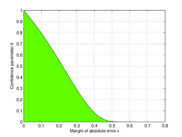
Figure 1: Region of $(\varepsilon,\delta)$

The improvement of our sample size bound (15) upon Chernoff-Hoeffding bound (13) is shown by Figure 2. It can be seen that for a typical requirement of confidence level $100(1-\delta)\%$ (e.g., $95\%$), the improvement can be $20\%$ to $30\%$.

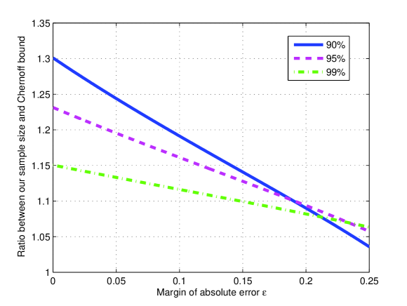
Figure 2: Comparison with Chernoff bound

Corollary 1 is also useful for the study of inverse binomial sampling. Let $\gamma$ be a positive integer. Define random number $\mathbf{n}$ as the minimum integer such that the summation of $\mathbf{n}$ consecutive Bernoulli random variables of common mean $p\in(0,1)$ is equal to $\gamma$. In other words, $\mathbf{n}$ is a random variable satisfying $\sum_{i=1}^{\mathbf{n}-1}X_{i}<\gamma=\sum_{i=1}^{\mathbf{n}}X_{i}$, where $X_{1},X_{2},\cdots$ are i.i.d. samples of Bernoulli random $X$ such that $\Pr\{X=1\}=1-\Pr\{X=0\}=p\in(0,1)$ as mentioned earlier. This means that $\mathbf{n}$ is the least number of Bernoulli trials of success rate $p\in(0,1)$ to come up with $\gamma$ successes. By virtue of Corollary 1, we have obtained the following results.

Corollary 2

$$\Pr\left\{\frac{\gamma}{\mathbf{n}}\leq z\right\}\leq\left(\frac{1}{2}+\varDelta\right)\exp\left(\frac{\gamma}{z}\mathscr{M}(z,p)\right)\qquad\text{for $z\in(0,p)$ such that $\frac{\gamma}{z}$ is an integer},$$

$$\Pr\left\{\frac{\gamma}{\mathbf{n}}\geq z\right\}\leq\left(\frac{1}{2}+\varDelta\right)\exp\left(\frac{\gamma}{z}\mathscr{M}(z,p)\right)\qquad\text{for $z\in(p,1)$ such that $\frac{\gamma}{z}$ is an integer},$$

where

$$\varDelta=\min\left\{\frac{1}{2},\frac{C_{\mathrm{BE}}[z^{2}+(1-z)^{2}]}{\sqrt{\gamma(1-z)}}\right\}.$$

Similar to the sample size problem associated with (13), it is an important problem to estimate the binomial parameter $p$ with a relative precision. Specifically, consider an inverse binomial sampling scheme as described above. Define $\widehat{\boldsymbol{p}}_{\gamma}=\frac{\gamma}{\mathbf{n}}$ as an estimator for $p$. A fundamental problem of practical importance is stated as follows:

Let $\varepsilon\in(0,1)$ and $\delta\in(0,1)$ be the margin of relative error and the confidence parameter respectively. How large $\gamma$ is sufficient to ensue

$$\Pr\left\{\left|\frac{\widehat{\boldsymbol{p}}_{\gamma}-p}{p}\right|<\varepsilon\right\}>1-\delta$$ (16)

for any $p\in(0,1)$?

By virtue of Corollary 2, we have established the following results regarding the above question.

Theorem 5

The following statements (I) and (II) hold true.

(I) $\Pr\left\{\left|\frac{\widehat{\boldsymbol{p}}_{\gamma}-p}{p}\right|<\varepsilon\right\}>1-\delta$ for any $p\in(0,1)$ provided that $\varepsilon>0,\;0<\delta<1$ and

$$\gamma>\frac{(1+\varepsilon)}{(1+\varepsilon)\ln(1+\varepsilon)-\varepsilon}\ln\frac{2}{\delta}.$$ (17)

(II) $\Pr\left\{\left|\frac{\widehat{\boldsymbol{p}}_{\gamma}-p}{p}\right|<\varepsilon\right\}>1-\delta$ for any $p\in(0,1)$ provided that $0<\varepsilon<1$,

$$0<\delta<\exp\left(-\frac{3\varepsilon^{3}(4+\varepsilon)+4\varepsilon(3+\varepsilon)\ln 2}{4(9-6\varepsilon-2\varepsilon^{2})}-\varepsilon\sqrt{\left[\frac{3\varepsilon^{2}(4+\varepsilon)+4(3+\varepsilon)\ln 2}{4(9-6\varepsilon-2\varepsilon^{2})}\right]^{2}+\frac{3(1+\varepsilon)(3+\varepsilon)\ln 2}{2(9-6\varepsilon-2\varepsilon^{2})}}\right)$$

and

$$\gamma>\frac{(1+\varepsilon)}{(1+\varepsilon)\ln(1+\varepsilon)-\varepsilon}\ln\frac{1+\zeta}{\delta},$$ (18)

where $\zeta=2C_{\mathrm{BE}}\sqrt{\frac{1}{m}+\frac{z}{m-z-mz}}$ with $m=\frac{2}{\varepsilon^{2}}\ln\frac{1}{\delta}$ and $z=1+\frac{2\varepsilon}{3+\varepsilon}-\frac{9}{(3+\varepsilon)^{2}}\frac{\ln\frac{1}{\delta}}{\ln\frac{2}{\delta}}$.

The domain of $(\varepsilon,\delta)$ for which our sample size bound (18) can be used is shown by Figure 3. Clearly, a sufficient but not necessary condition to use our formula (18) is $0<\varepsilon<\frac{3}{5},\;0<\delta<\frac{1}{4}$.

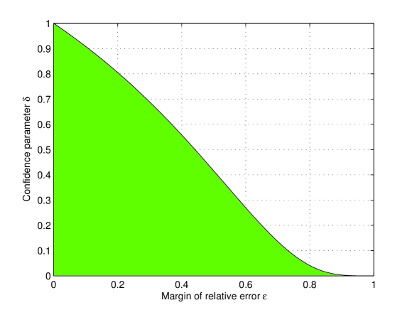
Figure 3: Region of $(\varepsilon,\delta)$

5.2 Negative Binomial Distribution

The probability mass function of a negative binomial random variable, $X$, is given by

$$f(x,\theta)\equiv\Pr\{X=x\mid p\}=\frac{\Gamma(x+r)}{\Gamma(x+1)\;\Gamma(r)}(1-p)^{x}p^{r}=h(x)\exp\left(\eta(\theta)T(x)-A(\theta)\right)\quad\text{for }x=0,1,2,\dots$$

where $r$ is a real, positive number,

$$T(x)=\frac{r+x}{r},\qquad h(x)=\frac{\Gamma(x+r)}{\Gamma(x+1)\;\Gamma(r)},\qquad\theta=\frac{1}{p},\qquad\eta(\theta)=r\ln\left(1-\frac{1}{\theta}\right),\qquad A(\theta)=r\ln(\theta-1).$$

Since $\frac{dA(\theta)}{d\theta}=\theta\frac{d\eta(\theta)}{d\theta}$ holds, by Theorem 3, we have the following result.

Corollary 3

Let $X_{1},\cdots,X_{n}$ be i.i.d. samples of negative binomial random variable $X$ parameterized by $\theta=\frac{1}{p}$. Then,

$$\Pr\left\{\sum_{i=1}^{n}T(X_{i})\geq nz\right\}\leq\left[\frac{pz-p}{1-p}\left(\frac{z-zp}{z-1}\right)^{z}\right]^{nr}\qquad\text{for $1>z\geq\theta=\frac{1}{p}$},$$

$$\Pr\left\{\sum_{i=1}^{n}T(X_{i})\leq nz\right\}\leq\left[\frac{pz-p}{1-p}\left(\frac{z-zp}{z-1}\right)^{z}\right]^{nr}\qquad\text{for $0<z\leq\theta=\frac{1}{p}$}.$$

5.3 Poisson Distribution

The probability mass function of a Poisson random variable, $X$, of mean value $\lambda$ is given by

$$f(x,\lambda)\equiv\Pr\{X=x\mid\lambda\}=\frac{\lambda^{x}e^{-\lambda}}{x!}=h(x)\exp\left(\eta(\lambda)T(x)-A(\lambda)\right),\qquad x\in\{0,1,2,\cdots\}$$

where

$$T(x)=x,\qquad h(x)=\frac{1}{x!},\qquad\eta(\lambda)=\ln\lambda,\qquad A(\lambda)=\lambda.$$

The moment generating function is $M(t)=\mathbb{E}[e^{tX}]=e^{-\lambda}\exp(\lambda e^{t})$. Clearly, $M^{\prime}(t)=\lambda e^{t}M(t)$ and $\mathbb{E}[X]=M^{\prime}(0)=\lambda$. It can be shown by induction that

$$\frac{d^{\ell+1}M(t)}{dt^{\ell+1}}=\left(1+2^{\ell-1}\lambda e^{t}\right)\frac{d^{\ell}M(t)}{dt^{\ell}},\qquad\mathbb{E}[X^{\ell+1}]=\left(1+2^{\ell-1}\lambda\right)\left.\frac{d^{\ell}M(t)}{dt^{\ell}}\right|_{t=0}=\lambda\prod_{i=1}^{\ell}\left(1+2^{i-1}\lambda\right)$$

for $\ell=1,2,\cdots$. Hence,

$$\mathbb{E}[|X-\lambda|^{2}]=\lambda,\qquad\mathbb{E}[|X-\lambda|^{4}]=\sum_{i=0}^{4}\binom{4}{i}(-\lambda)^{i}\mathbb{E}[X^{4-i}]=\lambda(3\lambda^{3}+8\lambda^{2}+3\lambda+1)$$

and

$$\frac{\mathbb{E}^{\frac{3}{4}}[|X-\lambda|^{4}]}{\mathbb{E}^{\frac{3}{2}}[|X-\lambda|^{2}]}=\left(3\lambda^{2}+8\lambda+3+\frac{1}{\lambda}\right)^{3/4}.$$ (19)

Since $\frac{dA(\lambda)}{d\lambda}=\lambda\frac{d\eta(\lambda)}{d\lambda}$ holds, making use of (19) and Theorem 2, we have the following results.

Corollary 4

Let $X_{1},\cdots,X_{n}$ be i.i.d. samples of Poisson random variable $X$ of mean value $\lambda$. Then,

$$\Pr\left\{\frac{\sum_{i=1}^{n}X_{i}}{n}\geq z\mid\lambda\right\}\leq\left(\frac{1}{2}+\varDelta\right)\left(\frac{\lambda^{z}e^{z}}{z^{z}e^{\lambda}}\right)^{n}\qquad\text{for $z\geq\lambda$},$$

$$\Pr\left\{\frac{\sum_{i=1}^{n}X_{i}}{n}\leq z\mid\lambda\right\}\leq\left(\frac{1}{2}+\varDelta\right)\left(\frac{\lambda^{z}e^{z}}{z^{z}e^{\lambda}}\right)^{n}\qquad\text{for $0<z\leq\lambda$},$$

where

$$\varDelta=\min\left\{\frac{1}{2},\frac{C_{\mathrm{BE}}}{\sqrt{n}}\left(3z^{2}+8z+3+\frac{1}{z}\right)^{\frac{3}{4}}\right\}.$$

5.4 Hypergeometric Distribution

The hypergeometric distribution can be described by the following model. Consider a finite population of $N$ units, of which there are $M$ units having a certain attribute. Draw $n$ units from the whole population by sampling without replacement. Let $K$ denote the number of units having the attribute found in the $n$ draws. Then, $K$ is a random variable possessing a hypergeometric distribution such that

$$\Pr\{K=k\}=\frac{\binom{M}{k}\binom{N-M}{n-k}}{\binom{N}{n}},\qquad k=0,1,\cdots,n.$$

It can be verified that

$$\frac{\Pr\{K=k+1\mid M_{1}\}}{\Pr\{K=k+1\mid M_{0}\}}\left[\frac{\Pr\{K=k\mid M_{1}\}}{\Pr\{K=k\mid M_{0}\}}\right]^{-1}=\frac{(M_{1}-k)(N-M_{0}-n+k+1)}{(M_{0}-k)(N-M_{1}-n+k+1)}\geq 1$$

for $M_{1}\geq M_{0}$, which implies that the hypergeometric distribution possesses the MLRP. Consequently, applying Theorem 1, we have the following results.

Corollary 5

Let $\widehat{M}=\widehat{M}(k)$ be a function of $k\in I_{K}$, which takes values in $\{m\in\mathbb{Z}:k\leq m\leq N\}$. Then,

$$\Pr\{K\leq k\mid M\}\leq\frac{\binom{M}{k}\binom{N-M}{n-k}}{\binom{\widehat{M}}{k}\binom{N-\widehat{M}}{n-k}}\quad\text{for $k\in I_{K}$ such that $\widehat{M}(k)\leq M$},$$

$$\Pr\{K\geq k\mid M\}\leq\frac{\binom{M}{k}\binom{N-M}{n-k}}{\binom{\widehat{M}}{k}\binom{N-\widehat{M}}{n-k}}\quad\text{for $k\in I_{K}$ such that $\widehat{M}(k)\geq M$}.$$

Actually, a specialized version of the inequalities in Corollary 5 had been used in the $15$-th version of our paper [3] published in arXiv on August 6, 2010 for developing multistage sampling schemes for estimating population proportion $p$. Moreover, the specialized inequalities had been used in the $20$-th version of our paper [4] published in arXiv on August 7, 2010 for developing multistage testing plans for hypotheses regarding $p$.

5.5 Hypergeometric Waiting-Time Distribution

The hypergeometric waiting-time distribution can be described by the following model. Consider a finite population of $N$ units, of which there are $M$ units having a certain attribute. Continue sampling until $r$ units of certain attribute is observed or the whole population is checked. Let $\boldsymbol{n}$ be the number of units checked when the sampling is stopped. Clearly, in the case of $r>M$, it must be true that $\Pr\{\boldsymbol{n}=N\}=1$, since the whole population is checked. In the case of $r\leq M$, the random variable $\boldsymbol{n}$ has a hypergeometric waiting-time distribution such that

$$\Pr\{\boldsymbol{n}=n\mid M\}=\frac{\binom{n-1}{r-1}\binom{N-n}{M-r}}{\binom{N}{M}}$$

for $r\leq M$ and $r\leq n\leq N$. It can be shown that

$$\frac{\Pr\{\boldsymbol{n}=n+1\mid M_{1}\}}{\Pr\{\boldsymbol{n}=n+1\mid M_{0}\}}\left[\frac{\Pr\{\boldsymbol{n}=n\mid M_{1}\}}{\Pr\{\boldsymbol{n}=n\mid M_{0}\}}\right]^{-1}=\frac{N-n-M_{1}+r}{N-n-M_{0}+r}\geq 1$$

for $M_{0}\leq M_{1}$, which implies that the hypergeometric waiting-time distribution possesses the MLRP. Hence, by virtue of Theorem 1, we have the following results.

Corollary 6

Let $\widehat{M}=\widehat{M}(n)$ be a function of $n\in I_{\boldsymbol{n}}$, which takes values in $\{m\in\mathbb{Z}:r\leq m\leq N\}$. Then,

$$\Pr\{\boldsymbol{n}\leq n\mid M\}\leq\frac{\binom{N}{\widehat{M}}\binom{N-n}{M-r}}{\binom{N}{M}\binom{N-n}{\widehat{M}-r}}=\frac{\binom{M}{r}\binom{N-M}{n-r}}{\binom{\widehat{M}}{r}\binom{N-\widehat{M}}{n-r}}\quad\text{for $n\in I_{\boldsymbol{n}}$ such that $\widehat{M}(n)\geq M$},$$

$$\Pr\{\boldsymbol{n}\geq n\mid M\}\leq\frac{\binom{N}{\widehat{M}}\binom{N-n}{M-r}}{\binom{N}{M}\binom{N-n}{\widehat{M}-r}}=\frac{\binom{M}{r}\binom{N-M}{n-r}}{\binom{\widehat{M}}{r}\binom{N-\widehat{M}}{n-r}}\quad\text{for $n\in I_{\boldsymbol{n}}$ such that $\widehat{M}(n)\leq M$}.$$

5.6 Normal Distribution

The probability density function of a Gaussian random variable, $X$, with mean $\mu$ and variance $\sigma^{2}$ is given by

$$f(x;\mu)=\frac{1}{\sqrt{2\pi}\sigma}\exp\left(-\frac{|x-\mu|^{2}}{2\sigma^{2}}\right)=h(x)\exp\left(\eta(\theta)T(x)-A(\theta)\right).$$

where

$$T(x)=\frac{x}{\sigma},\quad h(x)=\frac{1}{\sqrt{2\pi}\sigma}\exp\left(-\frac{x^{2}}{2\sigma^{2}}\right),\quad\theta=\frac{\mu}{\sigma},\quad A(\theta)=\frac{\theta^{2}}{2},\quad\eta(\theta)=\theta.$$

Since $\frac{dA(\theta)}{d\theta}=\theta\frac{d\eta(\theta)}{d\theta}$ holds, by Theorem 2, we have the following results.

Corollary 7

Let $X_{1},\cdots,X_{n}$ be i.i.d. samples of Gaussian random variable $X$ of mean $\mu$ and variance $\sigma^{2}$. Then,

$$\Pr\left\{\frac{\sum_{i=1}^{n}X_{i}}{n}\leq z\right\}<\frac{1}{2}\exp\left(-\frac{(z-\mu)^{2}}{2\sigma^{2}}\right)\qquad\text{for $z\leq\mu$},$$

$$\Pr\left\{\frac{\sum_{i=1}^{n}X_{i}}{n}\geq z\right\}<\frac{1}{2}\exp\left(-\frac{(z-\mu)^{2}}{2\sigma^{2}}\right)\qquad\text{for $z\geq\mu$}.$$

It should be noted that the inequalities in Corollary 7 may be shown by using other methods. However, the factor $\frac{1}{2}$ cannot be obtained by using Chernoff bounds.

5.7 Gamma Distribution

In probability theory and statistics, a random variable $X$ is said to have a gamma distribution if its density function is of the form

$$f(x)=\frac{x^{k-1}}{\Gamma(k)\theta^{k}}\exp\left(-\frac{x}{\theta}\right)=h(x)\exp\left(\eta(\theta)T(x)-A(\theta)\right)\;\;\;{\rm for}\;\;\;0<x<\infty$$

where $\theta>0,\;k>0$ are referred to as the scale parameter and shape parameter respectively, and

$$h(x)=\frac{x^{k-1}}{\Gamma(k)},\qquad T(x)=\frac{x}{k},\qquad\eta(\theta)=-\frac{k}{\theta},\qquad A(\theta)=k\ln\theta.$$

The moment generating function of $X$ is $M(t)=\mathbb{E}[e^{tX}]=(1-\theta t)^{-k}$ for $t<\frac{1}{\theta}$. It can be shown by induction that

$$\frac{d^{\ell+1}M(t)}{dt^{\ell+1}}=\frac{(k+\ell)\theta}{1-\theta t}\frac{d^{\ell}M(t)}{dt^{\ell}},\qquad\mathbb{E}[X^{\ell+1}]=(k+\ell)\theta\left.\frac{d^{\ell}M(t)}{dt^{\ell}}\right|_{t=0}=\theta^{\ell+1}\prod_{i=0}^{\ell}(k+i)$$

for $\ell=0,1,2,\cdots$. Therefore,

$$\mathbb{E}[|X-k\theta|^{2}]=k\theta^{2},\qquad\mathbb{E}[|X-k\theta|^{4}]=\sum_{i=0}^{4}\binom{4}{i}(-k\theta)^{i}\mathbb{E}[X^{4-i}]=3k(k+2)\theta^{4},$$

and

$$\frac{\mathbb{E}^{\frac{3}{4}}[|X-k\theta|^{4}]}{\mathbb{E}^{\frac{3}{2}}[|X-k\theta|^{2}]}=\left(3+\frac{6}{k}\right)^{\frac{3}{4}}.$$ (20)

Since $\frac{dA(\theta)}{d\theta}=\theta\frac{d\eta(\theta)}{d\theta}$ holds, making use of (20) and Theorem 2, we have

Corollary 8

Let $X_{1},\cdots,X_{n}$ be i.i.d. samples of Gamma random variable $X$ of shape parameter $k$ and scale parameter $\theta$. Then,

$$\Pr\left\{\frac{1}{n}\sum_{i=1}^{n}X_{i}\geq\rho k\theta\right\}\leq\left(\frac{1}{2}+\varDelta\right)\left[\rho\exp\left(1-\rho\right)\right]^{kn}\qquad\text{for $\rho\geq 1$},$$

$$\Pr\left\{\frac{1}{n}\sum_{i=1}^{n}X_{i}\leq\rho k\theta\right\}\leq\left(\frac{1}{2}+\varDelta\right)\left[\rho\exp\left(1-\rho\right)\right]^{kn}\qquad\text{for $0<\rho\leq 1$},$$

where

$$\varDelta=\min\left\{\frac{1}{2},\left(3+\frac{6}{k}\right)^{\frac{3}{4}}\frac{C_{\mathrm{BE}}}{\sqrt{n}}\right\}.$$

It should noted that the chi-square distribution of $k$ degrees of freedom is a special case of the Gamma distribution with shape parameter $\frac{k}{2}$ and scale parameter $2$. The exponential distribution of mean $\theta$ is also a special case of the Gamma distribution with shape parameter $1$ and scale parameter $\theta$. If the shape parameter $k$ is an integer, then the Gamma distribution represents an Erlang distribution. Therefore, the bounds in Corollary 8 can be used for those distributions.

Let $\widehat{\boldsymbol{\theta}}=\frac{\sum_{i=1}^{n}X_{i}}{kn}$. In order to find the sample size $n$ such that $\Pr\left\{\left|\widehat{\boldsymbol{\theta}}-\theta\right|<\varepsilon\theta\right\}>1-\delta$, we have established the following result.

Theorem 6

Let $\varepsilon>0$ and $0<\delta<1$. Then, $\Pr\left\{\left|\widehat{\boldsymbol{\theta}}-\theta\right|<\varepsilon\theta\right\}>1-\delta$ if $n>\frac{\ln\frac{1+\zeta}{\delta}}{k[\varepsilon+\ln(1+\varepsilon)]}$, where

$$\zeta=2C_{\mathrm{BE}}\left(3+\frac{6}{k}\right)^{\frac{3}{4}}\sqrt{\frac{k[\varepsilon+\ln(1+\varepsilon)]}{\ln\frac{1}{\delta}}}.$$

5.8 Student’s $t$-Distribution

If the random variable $X$ has a density function of the form

$$f(x)=\frac{\Gamma(\frac{n+1}{2})}{\sqrt{n\pi}\Gamma(\frac{n}{2})(1+\frac{x^{2}}{n})^{(n+1)/2}},\qquad\text{for}\quad-\infty<x<\infty,$$

then the variable $X$ is said to posses a Student’s $t$-distribution with $n$ degrees of freedom.

Now, we want to bound the tail probabilities of the distribution of $X$. Define $Y=\theta|X|$, where $\theta$ is a positive number. Then, $Y$ is a random variable parameterized by $\theta$. For any real number $t$,

$$\Pr\{Y\leq t\}=\Pr\left\{|X|\leq\frac{t}{\theta}\right\}=2\int_{0}^{\frac{t}{\theta}}f(x)dx-1.$$

By differentiation, we obtain the probability density function of $Y$ as $f_{Y}(t,\theta)=\frac{2}{\theta}f\left(\frac{t}{\theta}\right)$. Note that, for $\theta_{0}<\theta_{1}$,

$$\frac{f_{Y}(t,\theta_{1})}{f_{Y}(t,\theta_{0})}=\frac{\theta_{0}}{\theta_{1}}\frac{f\left(\frac{t}{\theta_{1}}\right)}{f\left(\frac{t}{\theta_{0}}\right)}=\frac{\theta_{0}}{\theta_{1}}\left(1+\frac{\frac{1}{\theta_{0}^{2}}-\frac{1}{\theta_{1}^{2}}}{\frac{n}{t^{2}}+\frac{1}{\theta_{1}^{2}}}\right)^{(n+1)/2},$$

which is monotonically increasing with respect to $t\in I_{Y}$. This implies that the likelihood ratio $\frac{f_{Y}(t,\theta_{1})}{f_{Y}(t,\theta_{0})}$ is monotonically increasing with respect to $Y$. Therefore, by Theorem 1,

$$\Pr\{|X|\geq x\}=\Pr\{Y\geq x\theta\}\leq\frac{\frac{2}{\theta}f\left(\frac{x\theta}{\theta}\right)}{\frac{2}{x\theta}f\left(\frac{x\theta}{x\theta}\right)}=\frac{xf(x)}{f(1)}=x\left(\frac{n+1}{n+x^{2}}\right)^{(n+1)/2}$$

for $x\geq 1$. Similarly,

$$\Pr\{|X|\leq x\}=\Pr\{Y\leq x\theta\}\leq\frac{\frac{2}{\theta}f\left(\frac{x\theta}{\theta}\right)}{\frac{2}{x\theta}f\left(\frac{x\theta}{x\theta}\right)}=\frac{xf(x)}{f(1)}=x\left(\frac{n+1}{n+x^{2}}\right)^{(n+1)/2}$$

for $0<x\leq 1$. By differentiation, we can show that the upper bound of the tail probabilities is unimodal with respect to $x$. In summary, we have the following results.

Corollary 9

Suppose $X$ possesses a Student’s $t$-distribution with $n$ degrees of freedom. Then,

$$\Pr\{|X|\geq x\}\leq x\left(\frac{n+1}{n+x^{2}}\right)^{(n+1)/2}\qquad\text{for $x\geq 1$},$$

$$\Pr\{|X|\leq x\}\leq x\left(\frac{n+1}{n+x^{2}}\right)^{(n+1)/2}\qquad\text{for $0\leq x\leq 1$},$$

where the upper bound of the tail probabilities is monotonically increasing with respect to $x\in(0,1)$ and monotonically decreasing with respect to $x\in(1,\infty)$.

5.9 Snedecor’s $F$-Distribution

If the random variable $X$ has a density function of the form

$$f(x)=\frac{\Gamma(\frac{n+m}{2})(\frac{m}{n})^{m/2}x^{(m-2)/2}}{\Gamma(\frac{m}{2})\Gamma(\frac{n}{2})(1+\frac{m}{n}x)^{(n+m)/2}},\qquad\text{for}\quad 0<x<\infty,$$

then the variable $X$ is said to posses an $F$-distribution with $m$ and $n$ degrees of freedom.

Now, we want to bound the tail probabilities of the distribution of $X$. Define $Y=\theta X$, where $\theta$ is a positive number. Then, $Y$ is a random variable parameterized by $\theta$. For any real number $t$,

$$\Pr\{Y\leq t\}=\Pr\left\{X\leq\frac{t}{\theta}\right\}=\int_{0}^{\frac{t}{\theta}}f(x)dx.$$

By differentiation, we obtain the probability density function of $Y$ as $f_{Y}(t,\theta)=\frac{1}{\theta}f\left(\frac{t}{\theta}\right)$. Note that, for $\theta_{0}<\theta_{1}$,

$$\frac{f_{Y}(t,\theta_{1})}{f_{Y}(t,\theta_{0})}=\frac{\theta_{0}}{\theta_{1}}\frac{f\left(\frac{t}{\theta_{1}}\right)}{f\left(\frac{t}{\theta_{0}}\right)}=\left(\frac{\theta_{0}}{\theta_{1}}\right)^{m/2}\left(1+\frac{\frac{1}{\theta_{0}}-\frac{1}{\theta_{1}}}{\frac{n}{mt}+\frac{1}{\theta_{1}}}\right)^{(n+m)/2},$$

which is monotonically increasing with respect to $t\in I_{Y}$. This implies that the likelihood ratio $\frac{f_{Y}(t,\theta_{1})}{f_{Y}(t,\theta_{0})}$ is monotonically increasing with respect to $Y$. Therefore, by Theorem 1,

$$\Pr\{X\geq x\}=\Pr\{Y\geq x\theta\}\leq\frac{\frac{1}{\theta}f\left(\frac{x\theta}{\theta}\right)}{\frac{1}{x\theta}f\left(\frac{x\theta}{x\theta}\right)}=\frac{xf(x)}{f(1)}=x^{m/2}\left(\frac{n+m}{n+mx}\right)^{(m+n)/2}$$

for $x\geq 1$. Similarly,

$$\Pr\{X\leq x\}=\Pr\{Y\leq x\theta\}\leq\frac{\frac{1}{\theta}f\left(\frac{x\theta}{\theta}\right)}{\frac{1}{x\theta}f\left(\frac{x\theta}{x\theta}\right)}=\frac{xf(x)}{f(1)}=x^{m/2}\left(\frac{n+m}{n+mx}\right)^{(m+n)/2}$$

for $0<x\leq 1$. By differentiation, we can show that the upper bound of the tail probabilities is unimodal with respect to $x$. Formally, we state the results as follows.

Corollary 10

Suppose $X$ possesses an $F$-distribution with $m$ and $n$ degrees of freedom. Then,

$$\Pr\{X\geq x\}\leq x^{m/2}\left(\frac{n+m}{n+mx}\right)^{(m+n)/2}\qquad\text{for $x\geq 1$},$$

$$\Pr\{X\leq x\}\leq x^{m/2}\left(\frac{n+m}{n+mx}\right)^{(m+n)/2}\qquad\text{for $0<x\leq 1$},$$

where the upper bound of the tail probabilities is monotonically increasing with respect to $x\in(0,1)$ and monotonically decreasing with respect to $x\in(1,\infty)$.

6 Using Probabilistic Inequalities for Parameter Estimation

In this section, we shall explore the general applications of the probabilistic inequalities for parameter estimation.

6.1 Interval Estimation

From Theorem 1, it can be seen that, for a large class of distributions, the likelihood ratio bounds of the cumulative distribution function and complementary cumulative distribution of random variable $\boldsymbol{\varphi}$ are partially monotone. Such monotonicity can be explored for the interval estimation of the underlying parameter $\theta$. In this direction, we have developed a method for constructing a confidence interval for $\theta$ as follows.

Theorem 7

Let $\boldsymbol{\varphi}$ be a random variable possessing a distribution determined by parameter $\theta\in\Theta$. Let $I_{\boldsymbol{\varphi}}$ denote the support of $\boldsymbol{\varphi}$. Let $\mathbb{F}(.,.)$ and $\mathbb{G}(.,.)$ be bivariate functions possessing the following properties:

(i) $\mathbb{F}(z,\vartheta)$ is non-increasing with respect to $\vartheta$ no less than $z\in I_{\boldsymbol{\varphi}}$;

(ii) $\mathbb{G}(z,\vartheta)$ is non-decreasing with respect to $\vartheta$ no greater than $z\in I_{\boldsymbol{\varphi}}$;

(iii)

$$\Pr\{\boldsymbol{\varphi}\leq z\mid\theta\}\leq\mathbb{F}(z,\theta)\quad\text{for $z$ no greater than }\;\theta\in\Theta,$$

$$\Pr\{\boldsymbol{\varphi}\geq z\mid\theta\}\leq\mathbb{G}(z,\theta)\quad\text{for $z$ no less than}\;\theta\in\Theta.$$

Let $\delta\in(0,1)$. Define confidence limits $L(\boldsymbol{\varphi},\delta)$ and $U(\boldsymbol{\varphi},\delta)$ as functions of $\boldsymbol{\varphi}$ and $\delta$ such that $\{\mathbb{F}(\boldsymbol{\varphi},U(\boldsymbol{\varphi},\delta))\leq\frac{\delta}{2},\;\mathbb{G}(\boldsymbol{\varphi},L(\boldsymbol{\varphi},\delta))\leq\frac{\delta}{2},\;L(\boldsymbol{\varphi},\delta)\leq\boldsymbol{\varphi}\leq U(\boldsymbol{\varphi},\delta)\}$ is a sure event. Then, $\Pr\{L(\boldsymbol{\varphi},\delta)\leq\theta\leq U(\boldsymbol{\varphi},\delta)\mid\theta\}\geq 1-\delta$ for any $\theta\in\Theta$.

See Appendix D for a proof. By the monotonicity of $\mathbb{F}(z,\theta)$ and $\mathbb{G}(z,\theta)$ with respect to $\theta$, we can obtain the lower and upper confidence limits $L(\boldsymbol{\varphi},\delta)$ and $U(\boldsymbol{\varphi},\delta)$ by a bisection approach. In the context of Theorem 1, $\mathbb{F}(z,\theta)$ and $\mathbb{G}(z,\theta)$ have the same expression $\mathscr{M}(z,\theta)$.

6.2 Asymptotically Tight Bound of Sample Size

Clearly, the likelihood ratio bound may be applied to the determination of sample size for parameter estimation. Since the likelihood ratio bound coincides with Chernoff bound for the exponential family, it is interesting to investigate the sample size issue in connection with Chernoff bound.

Let a population be denoted by a random variable $X$. Let $\mu$ be the mean of $X$. Suppose that the distribution of $X$ is parameterized by $\mu$. Suppose that the moment generating function $\mathbb{E}[e^{tX}]$ exists for any real number $t$. Let $\overline{X}_{n}=\frac{\sum_{i=1}^{n}X_{i}}{n}$, where $X_{1},\cdots,X_{n}$ are i.i.d. samples of random variable $X$. Chernoff bound asserts that

$$\Pr\{\overline{X}_{n}\leq\mu-\varepsilon\}\leq[\mathcal{F}(\mu-\varepsilon,\mu)]^{n},$$

$$\Pr\{\overline{X}_{n}\geq\mu+\varepsilon\}\leq[\mathcal{G}(\mu+\varepsilon,\mu)]^{n}$$

where

$$\mathcal{F}(\mu-\varepsilon,\mu)=\inf_{t<0}\mathbb{E}[e^{t(X-\mu+\varepsilon)}],\qquad\mathcal{G}(\mu+\varepsilon,\mu)=\inf_{t>0}\mathbb{E}[e^{t(X-\mu-\varepsilon)}].$$

Let $\varepsilon>0$ be a pre-specified margin of absolute error. Let $\delta>0$ be a pre-specified confidence parameter. It is a ubiquitous problem to estimate $\mu$ by its empirical mean $\overline{X}_{n}$ such that

$$\Pr\{|\overline{X}_{n}-\mu|<\varepsilon\}>1-\delta.$$

To guarantee the above requirement, it suffices to choose the sample size $n$ greater than

$$N_{c}(\delta)\stackrel{{\scriptstyle\mathrm{def}}}{{=}}\max\left\{\frac{\ln\frac{\delta}{2}}{\ln\mathcal{F}(\mu-\varepsilon,\mu)},\;\frac{\ln\frac{\delta}{2}}{\ln\mathcal{G}(\mu+\varepsilon,\mu)}\right\}.$$

It is of theoretical and practical importance to know tightness of such sample size bound. Let $N_{\mathrm{a}}(\delta)$ be the minimum sample size $n$ to guarantee $\Pr\{|\overline{X}-\mu|<\varepsilon\}>1-\delta$. We discover the following interesting result.

Theorem 8

$$\lim_{\delta\to 0}\frac{N_{\mathrm{c}}(\delta)}{N_{\mathrm{a}}(\delta)}=1.$$

See Appendix E for a proof. This theorem implies that, for high confidence estimation (i.e., small $\delta$), the sample size bound $N_{c}(\delta)$ can be quite tight.

7 Conclusion

In this paper, we have opened a new avenue for deriving probabilistic inequalities. Especially, we have established a fundamental connection between monotone likelihood ratio and tail probabilities. A unified theory has been developed for bounding the tail probabilities of the exponential family of distributions. Simple and sharp bounds are obtained for some other important distributions.

Appendix A Proof of Theorem 1

To prove inequalities (1) and (2), we shall focus on the case that $X_{1},\cdots,X_{n}$ are discrete random variables. First, we need to establish (1). For $z\in\mathscr{Z}$ such that $\vartheta(z)$ is no less than $\theta$, the inequality (1) is trivially true if $\mathscr{M}(z,\theta)$ is not bounded. It remains to consider the case that $\mathscr{M}(z,\theta)$ is bounded. By the MLRP assumption, for $z\in\mathscr{Z}$ such that $\vartheta(z)$ is no less than $\theta$, the likelihood ratio $\Lambda(y,\theta,\vartheta(z))$ is non-decreasing with respect to $y\in\mathscr{Z}$. In other words, the likelihood ratio $\Lambda(y,\vartheta(z),\theta)$ is non-increasing with respect to $y\in\mathscr{Z}$ provided that $\vartheta(z)\geq\theta$. Hence, for $z\in\mathscr{Z}$ such that $\vartheta(z)\geq\theta$, it must be true that $\Lambda(\varphi(x_{1},\cdots,x_{n}),\vartheta(z),\theta)\leq\Lambda(z,\vartheta(z),\theta)$ for all observation $(x_{1},\cdots,x_{n})$ of random tuple $(X_{1},\cdots,X_{n})$ such that $\varphi(x_{1},\cdots,x_{n})\geq z$. Moreover, since $\mathscr{M}(z,\theta)$ is bounded, it must be true that $f_{n}(x_{1},\cdots,x_{n};\vartheta(z))>0$ for all observation $(x_{1},\cdots,x_{n})$ of random tuple $(X_{1},\cdots,X_{n})$ such that $\varphi(x_{1},\cdots,x_{n})\geq z$ and $f_{n}(x_{1},\cdots,x_{n};\theta)>0$. It follows that

$$\Pr\{\boldsymbol{\varphi}\geq z\mid\theta\} = \sum_{\varphi(x_{1},\cdots,x_{n})\geq z\atop{f_{n}(x_{1},\cdots,x_{n};\theta)>0}}f_{n}(x_{1},\cdots,x_{n};\theta)$$

$$= \sum_{\varphi(x_{1},\cdots,x_{n})\geq z\atop{f_{n}(x_{1},\cdots,x_{n};\theta)>0}}\frac{f_{n}(x_{1},\cdots,x_{n};\theta)}{f_{n}(x_{1},\cdots,x_{n};\vartheta(z))}\times f_{n}(x_{1},\cdots,x_{n};\vartheta(z))$$

$$= \sum_{\varphi(x_{1},\cdots,x_{n})\geq z\atop{f_{n}(x_{1},\cdots,x_{n};\theta)>0}}\Lambda(\varphi(x_{1},\cdots,x_{n}),\vartheta(z),\theta)\times f_{n}(x_{1},\cdots,x_{n};\vartheta(z))$$

$$\leq \sum_{\varphi(x_{1},\cdots,x_{n})\geq z}\Lambda(\varphi(x_{1},\cdots,x_{n}),\vartheta(z),\theta)\times f_{n}(x_{1},\cdots,x_{n};\vartheta(z))$$

$$\leq \sum_{\varphi(x_{1},\cdots,x_{n})\geq z}\Lambda(z,\vartheta(z),\theta)\times f_{n}(x_{1},\cdots,x_{n};\vartheta(z))$$

$$= \Lambda(z,\vartheta(z),\theta)\sum_{\varphi(x_{1},\cdots,x_{n})\geq z}f_{n}(x_{1},\cdots,x_{n};\vartheta(z))$$

$$= \mathscr{M}(z,\theta)\times\Pr\{\boldsymbol{\varphi}\geq z\mid\vartheta(z)\}\leq\mathscr{M}(z,\theta)$$

for $z\in\mathscr{Z}$ such that $\vartheta(z)$ is no less than $\theta$. This establishes (1).

In order to show (2), it suffices to consider the case that $\mathscr{M}(z,\theta)$ is bounded, since the inequality (2) is trivially true if $\mathscr{M}(z,\theta)$ is not bounded. By the MLRP assumption, for $z\in\mathscr{Z}$ such that $\vartheta(z)$ is no greater than $\theta$, the likelihood ratio $\Lambda(y,\vartheta(z),\theta)$ is non-decreasing with respect to $y\in\mathscr{Z}$. Hence, for $z\in\mathscr{Z}$ such that $\vartheta(z)\leq\theta$, it must be true that $\Lambda(\varphi(x_{1},\cdots,x_{n}),\vartheta(z),\theta)\leq\Lambda(z,\vartheta(z),\theta)$ for all observation $(x_{1},\cdots,x_{n})$ of random tuple $(X_{1},\cdots,X_{n})$ such that $\varphi(x_{1},\cdots,x_{n})\leq z$. Moreover, since $\mathscr{M}(z,\theta)$ is bounded, it must be true that $f_{n}(x_{1},\cdots,x_{n};\vartheta(z))>0$ for all observation $(x_{1},\cdots,x_{n})$ of random tuple $(X_{1},\cdots,X_{n})$ such that $\varphi(x_{1},\cdots,x_{n})\leq z$ and $f_{n}(x_{1},\cdots,x_{n};\theta)>0$. It follows that

$$\Pr\{\boldsymbol{\varphi}\leq z\mid\theta\} = \sum_{\varphi(x_{1},\cdots,x_{n})\leq z\atop{f_{n}(x_{1},\cdots,x_{n};\theta)>0}}f_{n}(x_{1},\cdots,x_{n};\theta)$$

$$= \sum_{\varphi(x_{1},\cdots,x_{n})\leq z\atop{f_{n}(x_{1},\cdots,x_{n};\theta)>0}}\frac{f_{n}(x_{1},\cdots,x_{n};\theta)}{f_{n}(x_{1},\cdots,x_{n};\vartheta(z))}\times f_{n}(x_{1},\cdots,x_{n};\vartheta(z))$$

$$= \sum_{\varphi(x_{1},\cdots,x_{n})\leq z\atop{f_{n}(x_{1},\cdots,x_{n};\theta)>0}}\Lambda(\varphi(x_{1},\cdots,x_{n}),\vartheta(z),\theta)\times f_{n}(x_{1},\cdots,x_{n};\vartheta(z))$$

$$\leq \sum_{\varphi(x_{1},\cdots,x_{n})\leq z}\Lambda(\varphi(x_{1},\cdots,x_{n}),\vartheta(z),\theta)\times f_{n}(x_{1},\cdots,x_{n};\vartheta(z))$$

$$\leq \sum_{\varphi(x_{1},\cdots,x_{n})\leq z}\Lambda(z,\vartheta(z),\theta)\times f_{n}(x_{1},\cdots,x_{n};\vartheta(z))$$

$$= \Lambda(z,\vartheta(z),\theta)\sum_{\varphi(x_{1},\cdots,x_{n})\leq z}f_{n}(x_{1},\cdots,x_{n};\vartheta(z))$$

$$= \mathscr{M}(z,\theta)\times\Pr\{\boldsymbol{\varphi}\leq z\mid\vartheta(z)\}\leq\mathscr{M}(z,\theta)$$

for $z\in\mathscr{Z}$ such that $\vartheta(z)$ is no greater than $\theta$. This proves (2).

The proof of inequalities (1) and (2) for the case that $X_{1},\cdots,X_{n}$ are continuous variables can be completed by replacing the summation of probability mass functions with integration of probability density functions. It remains to show statements (i), (ii) and (iii).

Clearly, statement (i) is a direct consequence of assumptions (a), (b) and the definition of $\varphi(.)$. The monotonicity of $\mathscr{M}(z,\theta)$ with respect to $\theta$ as described by statement (ii) of the theorem can be established as follows. To show $\mathscr{M}(z,\theta_{2})\leq\mathscr{M}(z,\theta_{1})$ for $\theta_{2}>\theta_{1}\geq z$, note that

$$\mathscr{M}(z,\theta_{2})=\frac{g(z,\theta_{2})}{g(z,z)}\leq\frac{g(z,\theta_{1})}{g(z,z)}=\mathscr{M}(z,\theta_{1}),$$

where the inequality is due to the assumption that $g(z,\theta)$ is non-increasing with respect to $\theta$ no less than $z$. On the other hand, to show $\mathscr{M}(z,\theta_{1})\leq\mathscr{M}(z,\theta_{2})$ for $\theta_{1}<\theta_{2}\leq z$, note that

$$\mathscr{M}(z,\theta_{1})=\frac{g(z,\theta_{1})}{g(z,z)}\leq\frac{g(z,\theta_{2})}{g(z,z)}=\mathscr{M}(z,\theta_{2}),$$

where the inequality is due to the assumption that $g(z,\theta)$ is non-decreasing with respect to $\theta$ no greater than $z$. This justifies statement (ii) of the theorem.

Finally, consider the monotonicity of $\mathscr{M}(z,\theta)$ with respect to $z$ as described by statement (iii) of the theorem. To show $\mathscr{M}(z_{2},\theta)\leq\mathscr{M}(z_{1},\theta)$ for $z_{2}>z_{1}\geq\theta$, notice that

$$\mathscr{M}(z_{2},\theta)=\frac{g(z_{2},\theta)}{g(z_{2},z_{2})}\leq\frac{g(z_{2},\theta)}{g(z_{2},z_{1})}\leq\frac{g(z_{1},\theta)}{g(z_{1},z_{1})}=\mathscr{M}(z_{1},\theta),$$

where the first inequality is due to the assumption that $g(z,\theta)$ is non-decreasing with respect to $\theta$ no greater than $z$ and the second one is due to the assumption that $\Lambda(z,\theta_{0},\theta_{1})=\frac{g(z,\theta_{1})}{g(z,\theta_{0})}$ is non-decreasing with respect to $z$ provided that $\theta_{0}\leq\theta_{1}$. On the other side, to show $\mathscr{M}(z_{2},\theta)\geq\mathscr{M}(z_{1},\theta)$ for $z_{1}<z_{2}\leq\theta$, it suffices to observe that

$$\mathscr{M}(z_{1},\theta)=\frac{g(z_{1},\theta)}{g(z_{1},z_{1})}\leq\frac{g(z_{1},\theta)}{g(z_{1},z_{2})}\leq\frac{g(z_{2},\theta)}{g(z_{2},z_{2})}=\mathscr{M}(z_{2},\theta),$$

where the first inequality is due to the assumption that $g(z,\theta)$ is non-increasing with respect to $\theta$ no less than $z$ and the second one is due to the assumption that $\Lambda(z,\theta_{0},\theta_{1})=\frac{g(z,\theta_{1})}{g(z,\theta_{0})}$ is non-decreasing with respect to $z$ provided that $\theta_{0}\leq\theta_{1}$. Statement (iii) of the theorem is thus proved.

Appendix B Proof of Theorem 2

For simplicity of notations, define $F(z,\theta)=\Pr\{\varphi_{n}\leq z\mid\theta\}$ and $G(z,\theta)=\Pr\{\varphi_{n}\geq z\mid\theta\}$. By the assumption of the theorem, $\frac{f_{n}(X_{1},\cdots,X_{n};\theta)}{f_{n}(X_{1},\cdots,X_{n};\widehat{\theta}_{n})}=\Lambda(\varphi_{n},\widehat{\theta}_{n},\theta)$. By virtue of Theorem 1, we have

$$\Pr\left\{\frac{f_{n}(X_{1},\cdots,X_{n};\theta)}{f_{n}(X_{1},\cdots,X_{n};\widehat{\theta}_{n})}\leq\frac{\alpha}{2},\;\widehat{\theta}_{n}\leq\theta,\;\mid\theta\right\}=\Pr\left\{\Lambda(\varphi_{n},\widehat{\theta}_{n},\theta)\leq\frac{\alpha}{2},\;\widehat{\theta}_{n}\leq\theta\mid\theta\right\}$$

$$=\Pr\left\{\Lambda(\varphi_{n},\widehat{\theta}_{n},\theta)\leq\frac{\alpha}{2},\;\widehat{\theta}_{n}\leq\theta\mid\theta\right\}\leq\Pr\left\{F(\varphi_{n},\theta)\leq\frac{\alpha}{2},\;\widehat{\theta}_{n}\leq\theta\mid\theta\right\}$$

$$\leq\Pr\left\{F(\varphi_{n},\theta)\leq\frac{\alpha}{2}\mid\theta\right\}\leq\frac{\alpha}{2}$$

for any $\theta\in\Theta$. This proves (4). Similarly, for any $\theta\in\Theta$,

$$\Pr\left\{\frac{f_{n}(X_{1},\cdots,X_{n};\theta)}{f_{n}(X_{1},\cdots,X_{n};\widehat{\theta}_{n})}\leq\frac{\alpha}{2},\;\widehat{\theta}_{n}\geq\theta\mid\theta\right\}=\Pr\left\{\Lambda(\varphi_{n},\widehat{\theta}_{n},\theta)\leq\frac{\alpha}{2},\;\widehat{\theta}_{n}\geq\theta\mid\theta\right\}$$

$$=\Pr\left\{\Lambda(\varphi_{n},\widehat{\theta}_{n},\theta)\leq\frac{\alpha}{2},\;\widehat{\theta}_{n}\geq\theta\mid\theta\right\}\leq\Pr\left\{G(\varphi_{n},\theta)\leq\frac{\alpha}{2},\;\widehat{\theta}_{n}\geq\theta\mid\theta\right\}$$

$$\leq\Pr\left\{G(\varphi_{n},\theta)\leq\frac{\alpha}{2}\mid\theta\right\}\leq\frac{\alpha}{2},$$

which establishes (5). To show (6), making use of (4) and (5), we have

$$\Pr\left\{\frac{f_{n}(X_{1},\cdots,X_{n};\theta)}{f_{n}(X_{1},\cdots,X_{n};\widehat{\theta}_{n})}\leq\frac{\alpha}{2}\mid\theta\right\}$$

$$=\Pr\left\{\frac{f_{n}(X_{1},\cdots,X_{n};\theta)}{f_{n}(X_{1},\cdots,X_{n};\widehat{\theta}_{n})}\leq\frac{\alpha}{2},\;\widehat{\theta}_{n}\leq\theta\mid\theta\right\}+\Pr\left\{\frac{f_{n}(X_{1},\cdots,X_{n};\theta)}{f_{n}(X_{1},\cdots,X_{n};\widehat{\theta}_{n})}\leq\frac{\alpha}{2},\;\widehat{\theta}_{n}\geq\theta\mid\theta\right\}$$

$$\leq\frac{\alpha}{2}+\frac{\alpha}{2}=\alpha$$

for any $\theta\in\Theta$. To show (7), making use of (4), we have that

$$\Pr\left\{\frac{\sup_{\vartheta\in\mathscr{S}}f_{n}(X_{1},\cdots,X_{n};\vartheta)}{\sup_{\vartheta\in\Theta}f_{n}(X_{1},\cdots,X_{n};\vartheta)}\leq\frac{\alpha}{2},\;\widehat{\theta}_{n}\leq\inf\mathscr{S}\mid\theta\right\}$$

$$\leq\Pr\left\{\frac{\sup_{\vartheta\in\mathscr{S}}f_{n}(X_{1},\cdots,X_{n};\vartheta)}{\sup_{\vartheta\in\Theta}f_{n}(X_{1},\cdots,X_{n};\vartheta)}\leq\frac{\alpha}{2},\;\widehat{\theta}_{n}\leq\theta\mid\theta\right\}$$

$$\leq\Pr\left\{\frac{f_{n}(X_{1},\cdots,X_{n};\theta)}{\sup_{\vartheta\in\Theta}f_{n}(X_{1},\cdots,X_{n};\vartheta)}\leq\frac{\alpha}{2},\;\widehat{\theta}_{n}\leq\theta\mid\theta\right\}$$

$$=\Pr\left\{\frac{f_{n}(X_{1},\cdots,X_{n};\theta)}{f_{n}(X_{1},\cdots,X_{n};\widehat{\theta}_{n})}\leq\frac{\alpha}{2},\;\widehat{\theta}_{n}\leq\theta\mid\theta\right\}\leq\frac{\alpha}{2}$$

for any $\theta\in\mathscr{S}$. To show (8), making use of (5), we have that

$$\Pr\left\{\frac{\sup_{\vartheta\in\mathscr{S}}f_{n}(X_{1},\cdots,X_{n};\vartheta)}{\sup_{\vartheta\in\Theta}f_{n}(X_{1},\cdots,X_{n};\vartheta)}\leq\frac{\alpha}{2},\;\widehat{\theta}_{n}\geq\sup\mathscr{S}\mid\theta\right\}$$

$$\leq\Pr\left\{\frac{\sup_{\vartheta\in\mathscr{S}}f_{n}(X_{1},\cdots,X_{n};\vartheta)}{\sup_{\vartheta\in\Theta}f_{n}(X_{1},\cdots,X_{n};\vartheta)}\leq\frac{\alpha}{2},\;\widehat{\theta}_{n}\geq\theta\mid\theta\right\}$$

$$\leq\Pr\left\{\frac{f_{n}(X_{1},\cdots,X_{n};\theta)}{\sup_{\vartheta\in\Theta}f_{n}(X_{1},\cdots,X_{n};\vartheta)}\leq\frac{\alpha}{2},\;\widehat{\theta}_{n}\geq\theta\mid\theta\right\}$$

$$=\Pr\left\{\frac{f_{n}(X_{1},\cdots,X_{n};\theta)}{f_{n}(X_{1},\cdots,X_{n};\widehat{\theta}_{n})}\leq\frac{\alpha}{2},\;\widehat{\theta}_{n}\geq\theta\mid\theta\right\}\leq\frac{\alpha}{2}$$

for any $\theta\in\mathscr{S}$. To show (9), we use (6) to conclude that

$$\Pr\left\{\frac{\sup_{\vartheta\in\mathscr{S}}f_{n}(X_{1},\cdots,X_{n};\vartheta)}{\sup_{\vartheta\in\Theta}f_{n}(X_{1},\cdots,X_{n};\vartheta)}\leq\frac{\alpha}{2}\mid\theta\right\} \leq \Pr\left\{\frac{f_{n}(X_{1},\cdots,X_{n};\theta)}{\sup_{\vartheta\in\Theta}f_{n}(X_{1},\cdots,X_{n};\vartheta)}\leq\frac{\alpha}{2}\mid\theta\right\}$$

$$= \Pr\left\{\frac{f_{n}(X_{1},\cdots,X_{n};\theta)}{f_{n}(X_{1},\cdots,X_{n};\widehat{\theta}_{n})}\leq\frac{\alpha}{2}\mid\theta\right\}\leq\alpha$$

for any $\theta\in\mathscr{S}$. This completes the proof of the theorem.

Appendix C Proof of Theorem 3

Note that $\prod_{i=1}^{n}f_{X}(x_{i},\theta)=\left[\prod_{i=1}^{n}h(x_{i})\right]\times\exp\left(\eta(\theta)\sum_{i=1}^{n}T(x_{i})-nA(\theta)\right)$. By the assumption that $\frac{d\eta(\theta)}{d\theta}$ is positive for $\theta\in\Theta$, we have that the likelihood ratio

$$\Lambda(z,\theta_{0},\theta_{1})=\left[\frac{\exp\left(\eta(\theta_{1})z-A(\theta_{1})\right)}{\exp\left(\eta(\theta_{0})z-A(\theta_{0})\right)}\right]^{n}$$

is an increasing function of $z\in\Theta$ provided that $\theta_{0}<\theta_{1}$. Applying Theorem 1 with $\vartheta(z)=z$, we have

$$\Pr\{\widehat{\boldsymbol{\theta}}\geq z\mid\theta\}\leq\left[\frac{\exp\left(\eta(\theta)z-A(\theta)\right)}{\exp\left(\eta(z)z-A(z)\right)}\right]^{n}\times\Pr\{\widehat{\boldsymbol{\theta}}\geq z\mid z\}=\mathscr{M}(z,\theta)\times\Pr\{\widehat{\boldsymbol{\theta}}\geq z\mid z\}$$

for $z\in\Theta$ no less than $\theta\in\Theta$. Similarly, $\Pr\{\widehat{\boldsymbol{\theta}}\leq z\mid\theta\}\leq\mathscr{M}(z,\theta)\times\Pr\{\widehat{\boldsymbol{\theta}}\leq z\mid z\}$ for $z\in\Theta$ no greater than $\theta\in\Theta$. It remains to show statements (i)–(v) under the additional assumption that $\frac{A^{\prime}(\theta)}{\eta^{\prime}(\theta)}=\theta$. For simplicity of notations, define $w(z,\theta)=\exp\left(\eta(\theta)z-A(\theta)\right)$. Since $\frac{d\eta(\theta)}{d\theta}>0$ and $\frac{A^{\prime}(\theta)}{\eta^{\prime}(\theta)}=\theta$ for $\theta\in\Theta$, we have that

$$\frac{dw(z,\theta)}{d\theta}=(z-\theta)w(z,\theta)\frac{d\eta(\theta)}{d\theta},$$

which is positive for $\theta<z$ and negative for $\theta>z$. This implies that $w(z,\theta)$ is monotonically increasing with respect to $\theta$ less than $z$ and monotonically decreasing with respect to $\theta$ greater than $z$. Therefore, $\widehat{\boldsymbol{\theta}}$ must be a maximum-likelihood estimator of $\theta$.

Let $\psi(.)$ be the inverse function of $\eta(.)$ such that

$$\eta(\psi(\zeta))=\zeta$$ (21)

for $\zeta\in\{\eta(\theta):\theta\in\Theta\}$. Define compound function $B(.)$ such that $B(\zeta)=A(\psi(\zeta))$ for $\zeta\in\{\eta(\theta):\theta\in\Theta\}$. For simplicity of notations, we abbreviate $\psi(\zeta)$ as $\psi$ when this can be done without causing confusion. By the assumption that $\frac{dA(\theta)}{d\theta}=\theta\frac{d\eta(\theta)}{d\theta}$, we have

$$\frac{\frac{dA(\psi)}{d\psi}}{\frac{d\eta(\psi)}{d\psi}}=\psi.$$ (22)

Using (21), (22) and the chain rule of differentiation, we have

$$\frac{dB(\zeta)}{d\zeta}=\frac{dA(\psi)}{d\psi}\frac{d\psi}{d\zeta}=\frac{\frac{dA(\psi)}{d\psi}}{\frac{d\eta(\psi)}{d\psi}}\frac{d\eta(\psi)}{d\psi}\frac{d\psi}{d\zeta}=\frac{\frac{dA(\psi)}{d\psi}}{\frac{d\eta(\psi)}{d\psi}}\frac{d\eta(\psi)}{d\zeta}=\psi\frac{d\zeta}{d\zeta}=\psi(\zeta).$$ (23)

Putting $\zeta=\eta(\theta)$, we have

$$\mathbb{E}\left[\exp\left(nt(\widehat{\boldsymbol{\theta}})\right)\right]=\mathbb{E}\left[\exp\left(t\sum_{i=1}^{n}T(X_{i})\right)\right]=\int\cdots\int\prod_{i=1}^{n}\left[h(x_{i})\exp\left((\zeta+t)T(x_{i})-B(\zeta)\right)\right]dx_{1}\cdots dx_{n}$$

$$= \exp\left(nB(\zeta+t)-nB(\zeta)\right)\int\cdots\int\prod_{i=1}^{n}\left[h(x_{i})\exp\left((\zeta+t)T(x_{i})-B(\zeta+t)\right)\right]dx_{1}\cdots dx_{n}$$

$$= \exp\left(nB(\zeta+t)-nB(\zeta)\right).$$

By virtue of (23), the derivative of $nB(\zeta+t)-nB(\zeta)$ with respect to $t$ is

$$n\frac{dB(\zeta+t)}{dt}=n\psi(\zeta+t),$$

which is equal to $n\psi(\zeta)=n\theta$ for $t=0$. Thus, $\mathbb{E}[\widehat{\boldsymbol{\theta}}]=\theta$, which implies that $\widehat{\boldsymbol{\theta}}$ is also an unbiased estimator of $\theta$. This proves statement (i).

Again by virtue of (23), the derivative of $-tnz+nB(\zeta+t)-nB(\zeta)$ with respect to $t$ is

$$-nz+n\frac{dB(\zeta+t)}{dt}=-nz+n\psi(\zeta+t),$$

which is equal to $0$ for $t$ such that $\psi(\zeta+t)=z$ or equivalently, $\zeta+t=\eta(z)$, which implies $t=\eta(z)-\eta(\theta)$. Since $\mathbb{E}\left[\exp\left(nt(\widehat{\boldsymbol{\theta}}-z)\right)\right]$ is a convex function of $t$, its infimum with respect to $t\in\mathbb{R}$ is attained at $t=\eta(z)-\eta(\theta)$. It follows that

$$\inf_{t\in\mathbb{R}}\mathbb{E}\left[\exp\left(nt(\widehat{\boldsymbol{\theta}}-z)\right)\right]=\inf_{t\in\mathbb{R}}\exp\left(-tnz+nB(\zeta+t)-nB(\zeta)\right)$$

$$= \exp\left(-[\eta(z)-\eta(\theta)]nz+nB(\eta(z))-nB(\zeta)\right)=\exp\left(-[\eta(z)-\eta(\theta)]nz+nA(z)-nA(\theta)\right)$$

$$= \left[\frac{\exp\left(\eta(\theta)z-A(\theta)\right)}{\exp\left(\eta(z)z-A(z)\right)}\right]^{n}=\mathscr{M}(z,\theta).$$

Now, consider the monotonicity of $\mathscr{M}(z,\theta)$ with respect to $\theta$ as described by statement (iii) of the theorem. To show $\mathscr{M}(z,\theta_{2})\leq\mathscr{M}(z,\theta_{1})$ for $\theta_{2}>\theta_{1}\geq z$, note that

$$\mathscr{M}(z,\theta_{2})=\left[\frac{w(z,\theta_{2})}{w(z,z)}\right]^{n}\leq\left[\frac{w(z,\theta_{1})}{w(z,z)}\right]^{n}=\mathscr{M}(z,\theta_{1}),$$

where the inequality is due to the fact that $w(z,\theta)$ is non-increasing with respect to $\theta$ no less than $z$. On the other hand, to show $\mathscr{M}(z,\theta_{1})\leq\mathscr{M}(z,\theta_{2})$ for $\theta_{1}<\theta_{2}\leq z$, note that

$$\mathscr{M}(z,\theta_{1})=\left[\frac{w(z,\theta_{1})}{w(z,z)}\right]^{n}\leq\left[\frac{w(z,\theta_{2})}{w(z,z)}\right]^{n}=\mathscr{M}(z,\theta_{2}),$$

where the inequality is due to the fact that $w(z,\theta)$ is non-decreasing with respect to $\theta$ no greater than $z$. This justifies statement (iii) of the theorem.

Next, consider the monotonicity of $\mathscr{M}(z,\theta)$ with respect $z$ as described by statement (iv) of the theorem. To show $\mathscr{M}(z_{2},\theta)\leq\mathscr{M}(z_{1},\theta)$ for $z_{2}>z_{1}\geq\theta$, it is sufficient to note that

$$\mathscr{M}(z_{2},\theta)=\left[\frac{w(z_{2},\theta)}{w(z_{2},z_{2})}\right]^{n}\leq\left[\frac{w(z_{2},\theta)}{w(z_{2},z_{1})}\right]^{n}\leq\left[\frac{w(z_{1},\theta)}{w(z_{1},z_{1})}\right]^{n}=\mathscr{M}(z_{1},\theta),$$

where the first inequality is due to the fact that $w(z,\theta)$ is non-decreasing with respect to $\theta$ no greater than $z$ and the second one is due to the assumption that the likelihood ratio $\Lambda(z,\theta_{0},\theta_{1})=\left[\frac{w(z,\theta_{1})}{w(z,\theta_{0})}\right]^{n}$ is non-decreasing with respect to $z$. On the other side, to show $\mathscr{M}(z_{2},\theta)\geq\mathscr{M}(z_{1},\theta)$ for $z_{1}<z_{2}\leq\theta$, it suffices to observe that

$$\mathscr{M}(z_{1},\theta)=\left[\frac{w(z_{1},\theta)}{w(z_{1},z_{1})}\right]^{n}\leq\left[\frac{w(z_{1},\theta)}{w(z_{1},z_{2})}\right]^{n}\leq\left[\frac{w(z_{2},\theta)}{w(z_{2},z_{2})}\right]^{n}=\mathscr{M}(z_{2},\theta),$$

where the first inequality is due to the fact that $w(z,\theta)$ is non-increasing with respect to $\theta$ no less than $z$ and the second one is due to the assumption that the likelihood ratio $\Lambda(z,\theta_{0},\theta_{1})=\left[\frac{w(z,\theta_{1})}{w(z,\theta_{0})}\right]^{n}$ is non-decreasing with respect to $z$. Statement (iv) of the theorem is thus proved.

Finally, in order to show statement (v), notice that, in the course of proving that $\widehat{\boldsymbol{\theta}}$ is an unbiased estimator of $\theta$, we have shown that $\mathbb{E}[T(X)-\theta]=0$. Hence, applying the Berry-Essen inequality and Lyapounov’s inequality, we have that both (11) and (12) are true.

Appendix D Proof of Theorem 7

For simplicity of notations, define $F_{\boldsymbol{\varphi}}(z,\theta)=\Pr\{\boldsymbol{\varphi}\leq z\mid\theta\}$ and $G_{\boldsymbol{\varphi}}(z,\theta)=\Pr\{\boldsymbol{\varphi}\geq z\mid\theta\}$. By the assumption of the theorem, we have

$$F_{\boldsymbol{\varphi}}(z,\theta)\leq\mathbb{F}(z,\theta)\quad\text{for}\;z\leq\theta,$$ (24)

$$G_{\boldsymbol{\varphi}}(z,\theta)\leq\mathbb{G}(z,\theta)\quad\text{for}\;z\geq\theta.$$ (25)

Making use of (24), the assumption that $\mathbb{F}(z,\theta)$ is non-increasing with respect to $\theta\geq z$, and the assumption that $\{\mathbb{F}(\boldsymbol{\varphi},U(\boldsymbol{\varphi},\delta))\leq\frac{\delta}{2},\;\boldsymbol{\varphi}\leq U(\boldsymbol{\varphi},\delta)\}$ is a sure event, we have

$$\{U(\boldsymbol{\varphi},\delta)\leq\theta\}=\{\boldsymbol{\varphi}\leq U(\boldsymbol{\varphi},\delta)\leq\theta,\;\mathbb{F}(\boldsymbol{\varphi},U(\boldsymbol{\varphi},\delta))\leq\frac{\delta}{2}\}$$

$$\subseteq\{\boldsymbol{\varphi}\leq U(\boldsymbol{\varphi},\delta)\leq\theta,\;\mathbb{F}(\boldsymbol{\varphi},\theta)\leq\frac{\delta}{2}\}$$

$$\subseteq\{\boldsymbol{\varphi}\leq U(\boldsymbol{\varphi},\delta)\leq\theta,\;F_{\boldsymbol{\varphi}}(\boldsymbol{\varphi},\theta)\leq\frac{\delta}{2}\}\subseteq\{F_{\boldsymbol{\varphi}}(\boldsymbol{\varphi},\theta)\leq\frac{\delta}{2}\},$$

which implies that $\Pr\{U(\boldsymbol{\varphi},\delta)\leq\theta\}\leq\Pr\{F_{\boldsymbol{\varphi}}(\boldsymbol{\varphi},\theta)\leq\frac{\delta}{2}\}\leq\frac{\delta}{2}$. On the other hand, Making use of (25), the assumption that $\mathbb{G}(z,\theta)$ is non-decreasing with respect to $\theta\leq z$, and the assumption that $\{\mathbb{G}(\boldsymbol{\varphi},L(\boldsymbol{\varphi},\delta))\leq\frac{\delta}{2},\;\boldsymbol{\varphi}\geq L(\boldsymbol{\varphi},\delta)\}$ is a sure event, we have

$$\{L(\boldsymbol{\varphi},\delta)\geq\theta\}=\{\boldsymbol{\varphi}\geq L(\boldsymbol{\varphi},\delta)\geq\theta,\;\mathbb{G}(\boldsymbol{\varphi},L(\boldsymbol{\varphi},\delta))\leq\frac{\delta}{2}\}$$

$$\subseteq\{\boldsymbol{\varphi}\geq L(\boldsymbol{\varphi},\delta)\geq\theta,\;\mathbb{G}(\boldsymbol{\varphi},\theta)\leq\frac{\delta}{2}\}$$

$$\subseteq\{\boldsymbol{\varphi}\geq L(\boldsymbol{\varphi},\delta)\geq\theta,\;G_{\boldsymbol{\varphi}}(\boldsymbol{\varphi},\theta)\leq\frac{\delta}{2}\}\subseteq\{G_{\boldsymbol{\varphi}}(\boldsymbol{\varphi},\theta)\leq\frac{\delta}{2}\},$$

which implies that $\Pr\{L(\boldsymbol{\varphi},\delta)\geq\theta\}\leq\Pr\{G_{\boldsymbol{\varphi}}(\boldsymbol{\varphi},\theta)\leq\frac{\delta}{2}\}\leq\frac{\delta}{2}$. Finally, by virtue of the established fact that $\Pr\{U(\boldsymbol{\varphi},\delta)\leq\theta\}\leq\frac{\delta}{2}$ and $\Pr\{L(\boldsymbol{\varphi},\delta)\geq\theta\}\leq\frac{\delta}{2}$, we have $\Pr\{L(\boldsymbol{\varphi},\delta)<\theta<U(\boldsymbol{\varphi},\delta)\mid\theta\}\geq 1-\Pr\{U(\boldsymbol{\varphi},\delta)\leq\theta\}-\Pr\{L(\boldsymbol{\varphi},\delta)\geq\theta\}\geq 1-\frac{\delta}{2}-\frac{\delta}{2}=1-\delta$. This completes the proof of the theorem.

Appendix E Proof of Theorem 8

Let $N_{\mathrm{b}}(\delta)$ be the minimum sample size to ensure that

$$\Pr\{\overline{X}_{n}\geq\mu+\varepsilon\}\leq\frac{\delta}{2},\qquad\Pr\{\overline{X}_{n}\leq\mu-\varepsilon\}\leq\frac{\delta}{2}.$$

Since $\Pr\{|\overline{X}_{n}-\mu|\geq\varepsilon\}$ equals the summation of $\Pr\{\overline{X}_{n}\geq\mu+\varepsilon\}$ and $\Pr\{\overline{X}_{n}\leq\mu-\varepsilon\}$, we have that $\Pr\{|\overline{X}_{n}-\mu|\geq\varepsilon\}\leq\delta$ implies $\Pr\{\overline{X}_{n}\geq\mu+\varepsilon\}\leq\delta$ and $\Pr\{\overline{X}_{n}\leq\mu-\varepsilon\}\leq\delta$. Consequently,

$$N_{\mathrm{a}}(\delta)>N_{\mathrm{b}}(2\delta).$$

Since $\Pr\{\overline{X}_{n}\geq\mu+\varepsilon\}\leq\frac{\delta}{2}$ and $\Pr\{\overline{X}_{n}\leq\mu-\varepsilon\}\leq\frac{\delta}{2}$ together imply $\Pr\{|\overline{X}_{n}-\mu|\geq\varepsilon\}\leq\delta$, we have

$$N_{\mathrm{a}}(\delta)<N_{\mathrm{b}}(\delta).$$

Therefore, $N_{\mathrm{b}}(2\delta)<N_{\mathrm{a}}(\delta)<N_{\mathrm{b}}(\delta)$. We claim that $\lim_{\delta\to 0}\frac{N_{\mathrm{c}}(\delta)}{N_{\mathrm{b}}(\delta)}=1$. To show this claim, we define

$$Q^{+}=\frac{\ln\Pr\{\overline{X}_{n}\geq\mu+\varepsilon\}}{n}$$

and

$$Q^{-}=\frac{\ln\Pr\{\overline{X}_{n}\leq\mu-\varepsilon\}}{n}.$$

Then,

$$Q^{+}<0,\quad Q^{-}<0,\quad\ln\mathcal{F}(\mu-\varepsilon,\mu)<0,\quad\ln\mathcal{G}(\mu+\varepsilon,\mu)<0$$

and

$$N_{\mathrm{b}}(\delta)=\max\left\{\frac{\ln\frac{\delta}{2}}{Q^{+}},\;\frac{\ln\frac{\delta}{2}}{Q^{-}}\right\}.$$

It follows that

$$\lim_{\delta\to 0}\frac{N_{\mathrm{c}}(\delta)}{N_{\mathrm{b}}(\delta)}=\lim_{\delta\to 0}\frac{1}{N_{\mathrm{b}}(\delta)}\times\max\left\{\frac{\ln\frac{\delta}{2}}{\ln\mathcal{F}(\mu-\varepsilon,\mu)},\frac{\ln\frac{\delta}{2}}{\ln\mathcal{G}(\mu+\varepsilon,\mu)}\right\}$$

$$=\lim_{\delta\to 0}\frac{\max\{Q^{+},Q^{-}\}}{\max\{\ln\mathcal{F}(\mu-\varepsilon,\mu),\ln\mathcal{G}(\mu+\varepsilon,\mu)\}}.$$

By Chernoff’s theorem,

$$\lim_{\delta\to 0}Q^{+}=\ln\mathcal{G}(\mu+\varepsilon,\mu),\qquad\lim_{\delta\to 0}Q^{-}=\ln\mathcal{F}(\mu-\varepsilon,\mu)$$

and consequently,

$$\lim_{\delta\to 0}\max\{Q^{+},Q^{-}\}=\max\{\ln\mathcal{F}(\mu-\varepsilon,\mu),\;\ln\mathcal{G}(\mu+\varepsilon,\mu)\}$$

and the claim follows. Using the established claim, we have

$$\lim_{\delta\to 0}\frac{N_{\mathrm{b}}(\delta)}{N_{\mathrm{b}}(2\delta)}=\lim_{\delta\to 0}\left[\frac{N_{\mathrm{b}}(\delta)}{N_{\mathrm{c}}(\delta)}\times\frac{\max\left\{\frac{\ln\frac{\delta}{2}}{\ln\mathcal{F}(\mu+\varepsilon,\mu)},\frac{\ln\frac{\delta}{2}}{\ln\mathcal{G}(\mu-\varepsilon,\mu)}\right\}}{\max\left\{\frac{\ln\delta}{\ln\mathcal{F}(\mu+\varepsilon,\mu)},\frac{\ln\delta}{\ln\mathcal{G}(\mu-\varepsilon,\mu)}\right\}}\times\frac{N_{\mathrm{c}}(2\delta)}{N_{\mathrm{b}}(2\delta)}\right]=\lim_{\delta\to 0}\frac{\ln\frac{\delta}{2}}{\ln\delta}=1.$$

Recalling $N_{\mathrm{b}}(2\delta)<N_{\mathrm{a}}(\delta)<N_{\mathrm{b}}(\delta)$, we can conclude that $\lim_{\delta\to 0}\frac{N_{\mathrm{b}}(\delta)}{N_{\mathrm{a}}(\delta)}=1$. Finally, recalling the established claim that $\lim_{\delta\to 0}\frac{N_{\mathrm{c}}(\delta)}{N_{\mathrm{b}}(\delta)}=1$, the proof of the theorem is thus completed.

References

- [1]
- [2] A. C. Berry, “The accuracy of the Gaussian approximation to the sum of independent variates,” Trans. Amer. Math. Soc., vol. 49, no. 1, pp. 122–139, 1941.
- [3] X. Chen, “A new framework of multistage hypothesis tests,” arXiv.0809.3170[math.ST], multiple versions, first submitted in September 2008.
- [4] X. Chen, “A new framework of multistage estimation,” arXiv.0809.1241[math.ST], multiple versions, first submitted in September 2008.
- [5] X. Chen, “Likelihhod ratios and proabbility inequalities,” submitted for publication.
- [6] H. Chernoff, “A measure of asymptotic efficiency for tests of a hypothesis based on the sum of observations,” Ann. Math. Statist., vol. 23, pp. 493–507, 1952.
- [7] C.-G. Esseen, “On the Liapunoff limit of error in the theory of probability,” Ark. Mat. Astron. Fys., vol. A28, no. 9, pp. 1-19, 1942.
- [8] W. Hoeffding, “Probability inequalities for sums of bounded variables,” J. Amer. Statist. Assoc., vol. 58, pp. 13–29, 1963.
- [9] I. G. Shevtsova, “Sharpening of the upper bound of the absolute constant in the Berry-Esseen inequality,” Theor. Probab. Appl., vol. 51, no. 3, pp. 549–553, 2007.
- [10] Ilya Tyurin, “New estimates of the convergence rate in the Lyapunov theorem,” arXiv.0912.0726v1[math.PR], December, 2009.