Surface convection and red giants radii measurements

The phenomenological models of convection use characteristic length scales they do not determine but that are chosen to fit solar or stellar observations. We investigate if changes of these length scales are required between the Sun and low mass stars on the red giant branch (RGB). The question is addressed jointly in the frameworks of the mixing length theory and of the full spectrum of turbulence model. For both models, the convective length scale is assumed to be a fixed fraction of the local pressure scale height.

We use constraints coming from the observed effective temperatures and linear radii independently. We rely on a sample of 38 nearby giants and subgiants for which surface temperatures and luminosities are known accurately and the radii are determined through interferometry to better than 10%. For the few cases where the stellar masses were determined by asteroseismological measurements, we computed dedicated models. First we calibrate the solar models. Then, with the same physics, we compute RGB models for masses between $\rm 0.9M_{\odot}$ and $\rm 2.5M_{\odot}$ and metallicities ranging from $\rm[Fe/H]=-0.34$ to solar. The evolution is followed up to $\rm 10^{3}\,L_{\odot}$. A special attention is given to the opacities and to the non grey atmosphere models used as boundary conditions for which the model of convection is the same as in the interior.

We find that for both the mixing length theory and the full spectrum of turbulence model the characteristic solar length scale for convection has to be slightly reduced to fit the lower edge of the observed RGB. The corresponding models also better match the expected mass distribution on the RGB and are in better agreement to the seismic constraints. These results are robust whether effective temperatures determined spectroscopically or radii determined interferometrically are used.

1 Introduction

The modelling of solar and stellar surface convection requires hydrodynamical radiative transfer computations (Nordlund et al. aake09 (2009)). These tridimensional calculations are extremely time consuming because convection zones motions are characterized by short time scales and enormous turbulence. Therefore, in spite of the current computational power, the direct modelling of convection does not rely on first principles only but still necessitates simplifying assumptions.

Direct observations can constrain the properties of outer convection in stars. The Sun’s radius is routinely used to calibrate the main free parameter of the mixing length theory, $\rm\alpha_{mlt}$, the characteristic length scale of convection in this model being generaly $\rm\alpha_{mlt}H_{p}$ where $\rm H_{p}$ denotes the local pressure scale heigth. It is customary to consider that the solar $\rm\alpha_{mlt}$ applies all the way through stellar evolution and some recent studies have suggested this to be a valid hypothesis for low-mass red giant stars (Ferraro et al. ferraro06 (2006); VandenBerg et al. vdb08 (2008)). However hydrodynamical convection calculations (Ludwig et al. ludwig99 (1999)) show that slightly different $\rm\alpha_{mlt}$ should be used depending on the effective temperature (hereafter $\rm T_{eff}$) and the surface gravity (hereafter log g). Furthermore, the solar $\rm\alpha_{mlt}$ appears inappropriate to describe outer convection in red giants in the $\rm 3-20\,M_{\odot}$ mass range (Stothers & Chin stothers97 (1997)) and during the final stages of stellar evolution (D’Antona & Mazzitelli dantona96 (1996)). This is one reason why it is interesting to check what the nearby Galactic red giants can tell us about the mixing length theory (hereafter MLT). Besides the MLT there is another local treatment of convection that is increasingly used: the full spectrum of turbulence model (hereafter FST, Canuto, Goldman & Mazzitelli cgm96 (1996)). This approach is more physically consistent than the MLT and shows better agreement to numerous sets of observations (Mazzitelli mazzitelli99 (1999) and references therein, Samadi et al. sam06 (2006)).

As red giants and solar surface conditions ($\rm T_{eff}$, log g) strongly differ, they offer an adequate opportunity to check the MLT and the FST empirically. Such analyses were made in the recent years. However in the case of the nearby red giants, the usual observational constraints, absolute luminosity and $\rm T_{eff}$ are now supplemented by direct interferometric radii measurements and the new asterosesimic constraints. In this work we aim at using these new data to estimate $\rm\alpha_{mlt}$ and $\rm\alpha_{cgm}$ and their possible variation from the Sun to Galactic red giants. The analysis is made for both convection models using constraints on effective temperatures and radii independently. In section 7 we give the physical inputs to our stellar evolution code. We describe in detail the treatment of convection and the atmosphere modelling. In section 3 we present and discuss the observation sample. The calibration of the convective length scales relying on the Sun is made in section 4. Section 5 examines the MLT and the FST model of convection under the constraints coming from the red giant branch stars. We discuss our results and conclude in section 6.

2 The evolution code and the models

We use the CESAM code (Morel morel97 (1997)), an hydrostatic one dimensional stellar evolution code. However the standard version of CESAM is significantly modified here: to allow the computation of the stellar structure in the late stages of evolution we changed the usual integration variables of CESAM (see appendix 1). The evolution is computed from the zero age main sequence up to a luminosity of $\rm 10^{3}L_{\odot}$ on the red giant branch (hereafter RGB) for stars less massive than $\rm 2M_{\odot}$. For more massive stars, the models are evolved to the end of helium core burning on the early asymptotic giant branch (hereafter eAGB). The nuclear reaction rates are based on the NACRE compilation (Angulo et al. angulo99 (1999)). The network includes the proton-proton chains, the CNO cycle, and 3$\alpha$ and $\rm{}^{12}C(\alpha,\gamma)^{16}O$ reactions. The neutrino losses are computed according to the analytical fits of Itoh et al. (itoh96 (1996)). Microscopic diffusion is taken into account in the solar calibration models (§4) and more generally for all the models down to an effective temperature of 5000 K. This temperature roughly corresponds to the maximum extent in mass of the outer convection zone near the base of the RGB, the so-called first dredge up. Then because of the deep convective mixing, the subsequent evolution of diffusive and non diffusive models become undistinguishable (see Salaris et al. (salaris02 (2002)) and references herein) and diffusion is not taken into account below $\rm T_{eff}=5000K$.

The calculation of solar radius or RGB/eAGB radii models critically depends on the physical assumptions and inputs used in the outer layers. There are four of them.

i) The opacities: The low temperature opacities dominated by metallicity effects are critical in determining the effective temperature of giant stars at a given luminosity (Salaris et al. salaris02 (2002)). Below log T = 3.75 we use the data from Ferguson et al. (ferguson05 (2005)) (publicly available at http://webs.wichita.edu/physics/opacity/). In the higher temperature regime we use the OPAL opacities computed from the Lawrence Livermore National Laboratory web interface (http://physci.llnl.gov/Research/OPAL/new.html). Both opacity sets correspond to the solar metal repartition advocated by Asplund et al. (aspl05 (2005)). The electron conductive opacities that are only significant in the degenerate helium cores of red giants follow the Itoh et al. (itoh83 (1983)) prescription. We model stars well below the RGB tip and using the newer prescription of conductive opacities by Cassisi et al. (cassisi07 (2007)) would likely leave the evolution tracks unchanged as noticed by these authors.

ii) The convection: Two simplified local treatments of convection are investigated: the mixing length theory and the full spectrum of turbulence model. We chose a prescription of the MLT very similar to that of Böhm-Vitense (bohm58 (1958)) and whose exact description is given in the appendix of Piau et al. (piau05 (2005)). The formulation of the FST is that of Canuto, Goldman & Mazzitelli (cgm96 (1996)) and referred as CGM hereafter. The detailed equations are provided in the second appendix to this article. For the CGM approach, we adopt a characteristic length scale $\rm\Lambda=\alpha_{cgm}H_{p}$ in the equations -where $\rm H_{p}$ is the pressure scale height-. The CGM version we use is a simplified version rather than the true version of the CGM where $\rm\Lambda$ is the distance to the convection/radiation regime boundary. Finally we have two length scale parameters for the two treatments of convection: $\rm\alpha_{mlt}$ and $\rm\alpha_{cgm}$. In the occurence of convective cores, i.e. for stars more massive than $\rm 1.2M_{\odot}$, we assume convective overshooting ranging from $\rm 0.1H_{p}$ to $\rm 0.2H_{p}$ (Claret claret07 (2007)).

iii) The atmosphere modelling: We define the atmosphere as the region where the Rosseland optical depth is less than $\rm\tau_{b}=20$. The outer boundary conditions to the internal structure are taken at this depth where the diffusion equation becomes valid (Morel et al. morel94 (1994)). In late type stars, the convection straddles such an atmosphere/interior boundary and because the MLT and the CGM model predict different temperature gradients, it is important to use the same treatment of convection above and below this limit (Montalban et al. montal01 (2001), Montalban et al. montal04 (2004)). Besides this, molecular lines have a significant impact on atmosphere structures when $\rm T_{eff}<5000\leavevmode\nobreak\ K$. For these reasons we introduce two series of non grey atmosphere models as outer boundary conditions. The first series of temperature-optical depth relations ($\rm T(\tau)^{4}=T_{eff}^{4}f_{grid}(\tau)$) is computed with the PHOENIX/1D atmosphere code where the convection is handled using the MLT. The second series of temperature-optical depth relations is computed with the ATLAS12 atmosphere code (Castelli castelli05 (2005)). We modified ATLAS12 in order to use the CGM version of the FST model of convection instead of the MLT. The change is directly inspired from the implementation of the FST to the Atlas9 code by Kupka (kupka96 (1996)). The characteristic length scales adopted for the convection in both atmospheric sets is $\rm 0.5H_{p}$ as suggested by the solar and the cool dwarfs Balmer lines (Samadi et al. sam06 (2006); Gardiner et al. gardiner99 (1999)). Using the same convection model in the atmosphere and interior is necessary for consistency. In the proper treatment of the CGM, the convection length scale $\rm\Lambda$ is the distance to the convection/radiation regime boundary. This mimics the increase of the convective efficiency with depth (Heiter et al. hei02 (2002)) and the smooth change of the thermal gradient associated. However this treatment is not handled by our code where $\rm\Lambda=\alpha_{cgm}H_{p}$. In this framework, it is impossible to fit the solar radius when using in the interior the (small) atmosphere $\rm\alpha_{cgm}$ required by the Balmer lines. The sudden change in $\rm\alpha_{cgm}$ (or $\rm\alpha_{mlt}$) from the atmosphere to the interior should induce a discontinuity in the thermal gradient at the limit between the interior and the atmosphere. In order to smooth it out we perform a linear interpolation with optical depth on the temperature gradients: provided $\rm\nabla_{a}$ and $\rm\nabla_{i}$ are the temperature gradients ($\nabla=\frac{dlnT}{dlnP}$) computed using respectively the atmosphere and interior formalisms, we compute the gradient $\rm\nabla$ at the the optical depth $\rm\tau<\tau_{b}$ following:

$$\rm\nabla=(1-x(\tau))\nabla_{a}+x(\tau)\nabla_{i}$$

where $\rm x(\tau)=max(0,(\tau-1)/(\tau_{b}-1))$. Thus the atmospheric gradient is taken where $\rm\tau<1$, the interior gradient where $\rm\tau>\tau_{b}$ and and linear combination of them where $\rm 1<\tau<\tau_{b}$.

Both atmosphere grids were computed with the solar Asplund et al. (aspl05 (2005)) composition. In both of them there is a model every 100 K on the [4000,6400]K effective temperature range and every 0.5 on the [0.5,5.5] range of decimal logarithm of surface gravity (log g). For every stellar model we perform a linear interpolation in $\rm T_{eff}$ and log g using the four closest neighbours on the grid in order to get the $\rm f(\tau)$ theoretical relations. Together with $\rm T_{eff}$ this relation provides the temperature atmosphere profile: $\rm T(\tau)^{4}=T_{eff}^{4}f(\tau)$. For the most massive stars modelled, $\rm T_{eff}>6400\leavevmode\nobreak\ K$ on the main sequence and the $\rm f_{grid}(\tau)$ function is not available. In this case we use the $\rm f_{grid}(\tau)$ at 6400 K and for the closest log g.

iv) The equation of state (hereafter EOS): We use the OPAL 2005 EOS tables for Population I stars. Although the effect of the EOS is somewhat less important than the effects of opacities or atmosphere boundary conditions (Salaris et al. salaris02 (2002)) it still determines the temperature gradient in the convection zone and therefore affects the radius.

Let us make a final comment on the composition of the models before moving to the next section. The atmosphere $\rm T(\tau)$ relations are especially computed for the Asplund et al. (aspl05 (2005)) composition and metal repartition. The EOS and opacities both in low and high temperature regimes assume the same metal repartition. However we do not only consider the solar composition. The spectroscopic analyses of the red giants of our sample suggest them to have on average a slightly lower metallicity than the Sun and small but non negligible composition differences (§5.2). The total metal mass fraction Z and helium mass fraction Y are changed to explore the impact of composition.

3 The observations

The selection of our sample of stars was done in two steps. We first queried the CHARM2 catalogue (Richichi et al. richichi05 (2005)) to obtain all direct measurements of giant and subgiant angular diameters up to 2004, with effective temperatures in the range 5000 to 5500 K. The giants from Hutter et al.’s (hutter89 (1989)) Mark III survey were removed from the sample, as most of these measurements present strong biases due to calibration uncertainties (see their Sect. IV for details). We then searched the literature for more recent observations, and added the measurement of $\gamma$ Sge by Wittkowski et al. (wittkowski06 (2006)), $\delta$ Eri and $\xi$ Hya by Thévenin et al. (thevenin05 (2005)) and the recent high accuracy CHARA/FLUOR measurements of $\epsilon$ Oph (Mazumdar et al. mazumdar09 (2009)) and $\eta$ Ser (Mérand et al. merand09 (2009)). When several independent angular diameter measurements were available for the same star, we combined them into a single value taking into account their original error bars and the consistency of the different measurements. The conversion of uniform disk angular diameters to limb darkened values was done using linear limb darkening coefficients by Claret (claret95 (1995)), that are based on stellar atmosphere models by Kurucz (Kurucz kur93 (1993)). We are aware that the plane parallel ATLAS9 limb darkening coefficients by Claret (claret95 (1995)) are not optimal for cool, giant stars with low effective gravities, but the difference with PHOENIX models is very small for the selected sample. This difference amounts typically to a few per mille of the stellar size. Choosing the Claret (claret95 (1995)) values has the advantage of preserving the internal consistency of the sample, as the ATLAS9 models are the standard for the quoted interferometric measurements. A comparison of the measured angular diameters with predictions from the $F_{K}(V-K)$ surface brightness-color relations calibrated by Kervella et al. (2004a ) on Cepheid supergiants is presented in Fig. 1. The agreement is satisfactory within the uncertainties, with no systematic bias at a level of 2%. It is interesting to remark that these relations, established for supergiants, are mostly identical to the relations calibrated by Kervella et al. (2004b ) using dwarf and subgiants. This is an indication that the infrared surface brightness-color relations are universal for all classes of F-K stars.

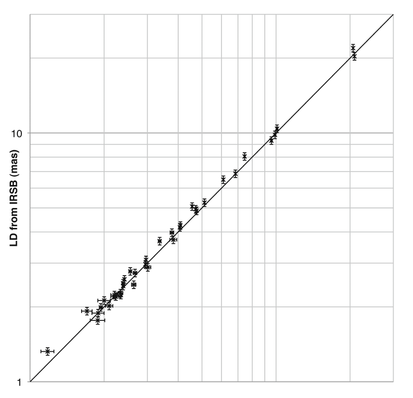
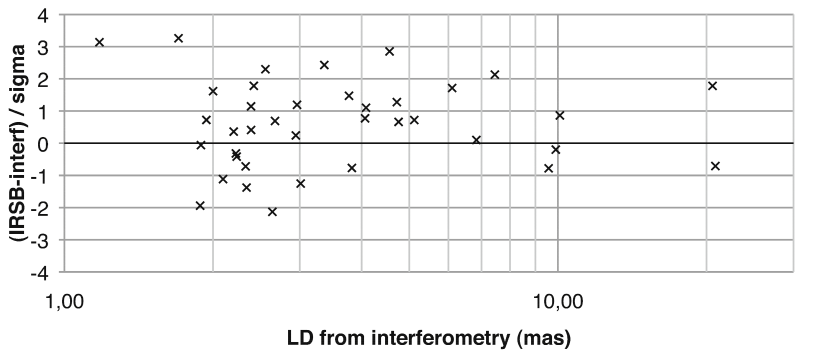
Figure 1: Comparison of the limb darkened angular diameters of the stars of our sample from direct interferometric measurements (horizontal axis) and photometric estimates based on the $F_{K}(V-K)$ infrared surface brightness-color relation (IRSB) from Kervella et al. (2004a ). The lower plot shows the residuals as a function of the measured angular diameter.

The spectroscopic effective temperature $\rm T_{eff}$, effective gravity $\log g$ and metallicity [Fe/H] of each star of our sample were taken from Cayrel de Strobel et al.’s (cayrel01 (2001)) catalogue, except for $\gamma$ Sge and $\xi$ Hya for which we used the $\rm T_{eff}$ values determined in the articles reporting their interferometric angular diameters. These estimates were originally obtained by McWilliam (mcwilliam90 (1990)), Thévenin & Idiart (thevenin99 (1999)) and Mallik (mallik98 (1998)). Similarly the $\rm T_{eff}$, metallicity and luminosity of $\epsilon$ Oph are adapted from De Ridder et al. (der06 (2006)) (also in agreement with Mazumdar et al. (mazumdar09 (2009))). The bolometric luminosity was estimated using the $K$ band photometry and the corresponding bolometric corrections $BC(K)$ by Houdashelt et al. (houdashelt00 (2000)). For $\gamma$ Sge, we extrapolated the $BC(K)$ value for $T_{\rm eff}=3805$ K (Wittkowski et al. wittkowski06 (2006)). For $\epsilon$ Oph and $\delta$ Eri, we adopted the $\rm T_{eff}$ metallicity and luminosity from De Ridder et al. (der06 (2006)) and Thevenin et al. (thevenin05 (2005)) respectively. To derive the linear radius, we used the parallaxes from the Hipparcos catalogue (esa97 (1997)). We kept only the stars for which the relative uncertainty on the linear radius is lower than 10%. The distances to the selected stars range from 11 to 110 pc. Thanks to this proximity, we neglected the interstellar reddening for the computation of the bolometric luminosity.

Our final sample contains 38 giant and subgiant stars with spectral types G5 to M0. It is interesting to remark that three stars of our sample have known asteroseismic oscillation frequencies: $\delta$ Eri, $\xi$ Hya, $\epsilon$ Oph. This allowed an accurate determination of their masses through a combination of their radius and the large frequency spacing (Thévenin et al. thevenin05 (2005); Mazumdar et al. mazumdar09 (2009)), that are estimated respectively to 1.215, 2.65 (no error bars mentioned by the authors) and $\rm 1.85\pm 0.05\,M_{\odot}$.

Table 1: Observational and physical parameters of our selected sample of giant and subgiant stars with interferometrically measured angular diameters.

Star	HD	Sp. Type	LD	$\pi$	Radius	$T_{\rm eff}$	$\log g$	[Fe/H]	$m_{V}$	$m_{K}$	BC($K$)	$M_{\rm bol}$	$L_{\rm bol}$
			(mas)	(mas)	($R_{\odot}$)	(K)							($L_{\odot}$)
$\mu$ Her	HD 161797	G5IV	$1.94\pm 0.03$	$119.05\pm 0.62$	$1.75\pm 0.03$	$5520$	$3.70$	$0.04$	$3.41$	$1.74$	$1.56$	$3.68\pm 0.05$	$2.7\pm 0.1$
$\delta$ Eri	HD 23249	K0IV	$2.39\pm 0.03$	$110.58\pm 0.88$	$2.32\pm 0.03$	$5055$	$3.79$	$0.13$	$3.51$	$1.40$	$1.84$	$3.46\pm 0.05$	$3.3\pm 0.2$
$\beta$ Aql	HD 188512	G8IV	$2.23\pm 0.10$	$72.95\pm 0.83$	$3.28\pm 0.15$	$5100$	$3.60$	$-0.30$	$3.71$	$1.65$	$1.84$	$2.81\pm 0.06$	$6.0\pm 0.3$
$\eta$ Cep	HD 198149	K0IV	$2.67\pm 0.04$	$69.73\pm 0.49$	$4.12\pm 0.07$	$4950$	$3.41$	$-0.32$	$3.41$	$1.22$	$1.84$	$2.28\pm 0.05$	$9.7\pm 0.5$
$\eta$ Ser	HD 168723	K0III-IV	$2.94\pm 0.01$	$53.93\pm 0.18$	$5.87\pm 0.03$	$4890$	$3.21$	$-0.42$	$3.26$	$1.05$	$1.84$	$1.55\pm 0.05$	$19\pm 1$
46 Lmi	HD 94264	K0III	$2.56\pm 0.03$	$33.40\pm 0.78$	$8.22\pm 0.22$	$4670$	$2.96$	$-0.20$	$3.83$	$1.30$	$2.00$	$0.91\pm 0.07$	$34\pm 2$
$\sigma$ Gem	HD 62044	K1III	$2.33\pm 0.05$	$26.68\pm 0.79$	$9.38\pm 0.35$	$4500$	$2.40$	$-0.02$	$4.28$	$1.74$	$2.16$	$1.03\pm 0.08$	$31\pm 2$
$\epsilon$ Aql	HD 176411	K1III	$2.00\pm 0.12$	$21.22\pm 0.77$	$10.14\pm 0.70$	$4760$	$2.91$	$0.00$	$4.03$	$1.79$	$2.00$	$0.42\pm 0.09$	$54\pm 5$
37 Tau	HD 25604	K0III	$1.70\pm 0.09$	$18.04\pm 0.84$	$10.15\pm 0.69$	$4700$	$2.77$	$0.01$	$4.35$	$2.03$	$2.00$	$0.31\pm 0.11$	$60\pm 6$
$\xi$ Hya	HD 100407	G7III	$2.39\pm 0.02$	$25.23\pm 0.83$	$10.18\pm 0.35$	$5037$	$2.83$	$-0.04$	$3.54$	$1.45$	$1.84$	$0.30\pm 0.09$	$60\pm 5$
$\epsilon$ Oph	HD 146791	G9.5IIIb	$2.96\pm 0.01$	$30.62\pm 0.20$	$10.39\pm 0.07$	$4955$	$2.89$	$-0.27$	$3.24$	$0.98$	$1.84$	$0.25\pm 0.05$	$63\pm 3$
$\delta$ Ari	HD 19787	K2III	$1.88\pm 0.13$	$19.44\pm 1.23$	$10.42\pm 0.97$	$4810$	$2.93$	$-0.03$	$4.35$	$2.17$	$2.00$	$0.61\pm 0.14$	$45\pm 6$
$\o$ CrB	HD 136512	K0III	$1.18\pm 0.07$	$11.90\pm 0.74$	$10.64\pm 0.93$	$4730$	$2.75$	$-0.44$	$5.52$	$2.93$	$2.00$	$0.30\pm 0.14$	$60\pm 8$
$\epsilon$ Cyg	HD 197989	K0III	$4.56\pm 0.02$	$45.26\pm 0.53$	$10.82\pm 0.14$	$4730$	$2.89$	$-0.27$	$2.50$	$-0.01$	$2.00$	$0.26\pm 0.06$	$62\pm 3$
$\delta$ Tau	HD 27697	K0III	$2.20\pm 0.07$	$21.29\pm 0.93$	$11.12\pm 0.61$	$4810$	$2.93$	$-0.03$	$3.76$	$1.64$	$2.00$	$0.28\pm 0.11$	$62\pm 6$
39 ari	HD 17361	K1.5III	$1.89\pm 0.11$	$18.06\pm 0.84$	$11.26\pm 0.82$	$4600$	$2.85$	$-0.02$	$4.51$	$2.10$	$2.16$	$0.54\pm 0.11$	$48\pm 5$
$\delta^{1}$ Tau	HD 27697	K0III	$2.34\pm 0.02$	$21.29\pm 0.93$	$11.81\pm 0.53$	$4030$	$1.83$	$-0.29$	$3.76$	$1.64$	$2.51$	$0.79\pm 0.11$	$39\pm 4$
12 Aql	HD 176678	K1III	$2.42\pm 0.01$	$21.95\pm 0.92$	$11.85\pm 0.50$	$4600$	$2.75$	$-0.19$	$4.03$	$1.47$	$2.16$	$0.34\pm 0.10$	$58\pm 6$
$\delta$ And	HD 3627	K3III	$4.09\pm 0.02$	$32.19\pm 0.68$	$13.64\pm 0.30$	$4360$	$2.37$	$0.04$	$3.28$	$0.47$	$2.16$	$0.17\pm 0.07$	$68\pm 4$
$\alpha$ Ari	HD 12929	K2III	$6.84\pm 0.02$	$49.48\pm 0.99$	$14.85\pm 0.30$	$4480$	$2.57$	$-0.25$	$2.00$	$-0.63$	$2.16$	$-0.15\pm 0.07$	$91\pm 6$
$\rho$ Boo	HD 127665	K3III	$3.82\pm 0.12$	$21.92\pm 0.81$	$18.75\pm 0.92$	$4260$	$2.22$	$-0.17$	$3.58$	$0.76$	$2.33$	$-0.21\pm 0.09$	$96\pm 9$
$\psi$ Uma	HD 96833	K1III	$4.07\pm 0.03$	$22.21\pm 0.68$	$19.68\pm 0.62$	$4550$	$2.53$	$-0.13$	$3.01$	$0.43$	$2.16$	$-0.68\pm 0.08$	$148\pm 12$
$\upsilon$ Per	HD 9927	K3III	$3.77\pm 0.06$	$18.76\pm 0.74$	$21.61\pm 0.93$	$4380$	$2.34$	$0.00$	$3.57$	$0.65$	$2.16$	$-0.83\pm 0.10$	$170\pm 16$
24 Per	HD 18449	K2III	$2.10\pm 0.07$	$9.31\pm 0.78$	$24.21\pm 2.19$	$4340$	$2.37$	$-0.19$	$4.95$	$2.10$	$2.33$	$-0.73\pm 0.18$	$155\pm 28$
$\alpha$ Boo	HD 124897	K1.5III	$20.84\pm 0.03$	$88.85\pm 0.74$	$25.21\pm 0.21$	$4345$	$2.05$	$-0.37$	$-0.04$	$-2.91$	$2.16$	$-1.01\pm 0.05$	$201\pm 10$
91 Psc	HD 8126	K5III	$2.23\pm 0.06$	$9.49\pm 0.82$	$25.30\pm 2.29$	$4090$	$1.93$	$-0.17$	$5.24$	$2.03$	$2.51$	$-0.58\pm 0.19$	$135\pm 25$
39 Cyg	HD 194317	K3III	$3.01\pm 0.08$	$12.77\pm 0.62$	$25.35\pm 1.41$	$4230$	$2.16$	$-0.17$	$4.44$	$1.39$	$2.33$	$-0.75\pm 0.11$	$159\pm 18$
11 Lac	HD 214868	K2III	$2.64\pm 0.05$	$10.81\pm 0.56$	$26.24\pm 1.46$	$4440$	$2.32$	$-0.25$	$4.51$	$1.67$	$2.16$	$-1.00\pm 0.12$	$200\pm 23$
31 Leo	HD 87837	K4III	$3.36\pm 0.04$	$11.89\pm 0.72$	$30.40\pm 1.88$	$4040$	$1.81$	$-0.02$	$4.38$	$0.98$	$2.51$	$-1.14\pm 0.14$	$227\pm 31$
$\upsilon$ Boo	HD 120477	K5.5III	$4.75\pm 0.04$	$13.29\pm 0.81$	$38.44\pm 2.37$	$3890$	$1.55$	$-0.23$	$4.05$	$0.44$	$2.51$	$-1.44\pm 0.14$	$299\pm 40$
$\beta$ Umi	HD 131873	K4III	$10.09\pm 0.08$	$25.79\pm 0.52$	$42.06\pm 0.91$	$4030$	$1.83$	$-0.29$	$2.08$	$-1.29$	$2.51$	$-1.73\pm 0.07$	$390\pm 25$
$\alpha$ Tau	HD 29139	K5III	$20.57\pm 0.02$	$50.09\pm 0.95$	$44.13\pm 0.84$	$3910$	$1.59$	$-0.34$	$0.86$	$-2.81$	$2.51$	$-2.04\pm 0.06$	$518\pm 32$
$\gamma$ Dra	HD 164058	K5III	$9.90\pm 0.09$	$22.10\pm 0.46$	$48.15\pm 1.09$	$3930$	$1.55$	$-0.14$	$2.23$	$-1.16$	$2.51$	$-1.93\pm 0.07$	$471\pm 30$
$\beta$ Cnc	HD 69267	K4III	$5.12\pm 0.02$	$11.23\pm 0.97$	$48.96\pm 4.23$	$4010$	$1.71$	$-0.24$	$3.54$	$0.19$	$2.51$	$-2.05\pm 0.19$	$526\pm 99$
$\alpha$ Lyn	HD 80493	K7III	$7.45\pm 0.04$	$14.69\pm 0.81$	$54.50\pm 3.02$	$3880$	$1.51$	$-0.26$	$3.13$	$-0.61$	$2.51$	$-2.32\pm 0.13$	$673\pm 83$
$\gamma$ Sge	HD 189319	M0III	$6.10\pm 0.02$	$11.90\pm 0.71$	$55.13\pm 3.29$	$3805$	$1.55$	$-0.14$	$3.53$	$-0.16$	$2.66$	$-2.13\pm 0.14$	$562\pm 75$
$\alpha$ Hya	HD 81797	K3II-III	$9.58\pm 0.08$	$18.40\pm 0.78$	$55.93\pm 2.41$	$4120$	$1.77$	$-0.12$	$2.00$	$-1.13$	$2.33$	$-2.48\pm 0.10$	$780\pm 78$
$\nu$ UMa	HD 98262	K3III	$4.72\pm 0.03$	$8.88\pm 0.64$	$57.07\pm 4.13$	$4070$	$1.89$	$-0.04$	$3.50$	$0.28$	$2.51$	$-2.47\pm 0.16$	$775\pm 122$

• $\theta_{\rm LD}$ is the limb darkened angular diameter measured by interferometry, taken from the CHARM2 catalogue compiled by Richichi et al. (richichi05 (2005)), except for $\gamma$ Sge (Wittkowski et al. wittkowski06 (2006)), $\delta$ Eri and $\xi$ Hya (Thévenin et al. thevenin05 (2005)), $\epsilon$ Oph (Mazumdar et al. mazumdar09 (2009)) and $\eta$ Ser (Mérand et al. merand09 (2009)).

• The parallax $\pi$ is taken from the original Hipparcos catalogue (ESA esa97 (1997)).

• $T_{\rm eff}$, $\log g$ and [Fe/H] are taken from Cayrel de Strobel et al. (cayrel01 (2001)), except for $\gamma$ Sge, $\delta$ Eri, $\epsilon$ Oph and $\xi$ Hya (see text).

• $m_{V}$ and $m_{K}$ were taken from SIMBAD.

• The uncertainty on the $K$ band bolometric correction $BC(K)$ (taken from Houdashelt et al. houdashelt00 (2000), except for $\gamma$ Sge) is taken uniformly equal to 0.05.

• The absolute bolometric magnitude of the Sun is $M_{\rm bol}(\odot)=4.75$.

4 Convection length scales from the Sun

The convection length scales can be calibrated using the Sun, as is customarily done. We assume $\rm L_{\odot}=3.846\,10^{33}erg.s^{-1}$ and $\rm R_{\odot}=6.9599\,10^{10}cm$ and start the solar evolution on the zero age main sequence. The calibration in luminosity, radius and metal to hydrogen ratio $\rm\frac{Z_{surf}}{X_{surf}}$ are achieved to better than $10^{-4}$ at the age of 4.6 Gyr for both MLT and CGM convection prescriptions. We consider the solar abundances and metal repartition of Asplund et al. (2005) therefore $\rm\frac{Z_{surf}}{X_{surf}}=1.65\,10^{-2}$. The microscopic diffusion is accounted for following Proffitt and Michaud (proffitt93 (1993)) It induces a decrease in helium and metal surface fractions in the course of the solar main sequence.

In the MLT framework we obtain $\rm\alpha_{mlt\odot}$=1.98. The initial composition of the calibrated solar model is $\rm X_{o}=0.7284$, $\rm Y_{o}=0.2578$ and $\rm Z_{o}=1.38\,10^{-2}$ and its solar age surface composition is $\rm X_{surf}=0.7592$ and $\rm Y_{surf}=0.2282$. The $\rm\alpha_{mlt\odot}$ is compatible with the recent estimate of VandenBerg et al. (vdb08 (2008)) also using non grey atmospheres as boundary conditions. Using the MARCS atmosphere models (Gustafsson et al. gus03 (2003)) the latter authors find $\rm\alpha_{mlt\odot}$=2.01. Samadi et al. (sam06 (2006)) using the Kurucz atmosphere models (Kurucz kur93 (1993), see also Heiter et al. hei02 (2002)) find $\rm\alpha_{mlt\odot}$=2.53. This larger value is likely due to the fact that Samadi et al. start interpolating between the atmosphere and interior gradients at the optical depth $\rm\tau=4$ whereas we start at $\rm\tau=1$ (see section 7). The overadiabaticity induced by the atmosphere $\rm\alpha=0.5$ extends over a larger region in their models and has to be compensated by a more efficient convection deeper. We recall that $\rm\alpha_{mlt\odot}$ depends on the assumed solar composition. For the Grevesse & Sauval (gs98 (1998)) composition ($\rm\frac{Z_{surf}}{X_{surf}}=2.3\,10^{-2}$) calibrated Sun, we find $\rm\alpha_{mlt\odot}$=1.67.

In the CGM model framework we obtain $\rm\alpha_{cgm\odot}$=0.77. The initial composition of the calibrated CGM solar model is nearly the same as for the calibrated MLT solar model. $\rm Z_{o}=1.38\,10^{-2}$ is identical while the hydrogen and helium fractions very slightly differ from the MLT case: $\rm X_{o}=0.7280$ and $\rm Y_{o}=0.2582$. So is the current surface composition with $\rm X_{surf}=0.7587$ and $\rm Y_{surf}=0.22865$. Our $\rm\alpha_{cgm\odot}$ is in close agreement with the values of authors who used the same formulation of the CGM. Bernkopf (bernkopf98 (1998)) finds $\rm\alpha_{cgm\odot}=0.82$ and Samadi et al. (sam06 (2006)) find $\rm\alpha_{cgm\odot}=0.78$.

Theoretical atmosphere models probably account properly for the differential changes in the outer stellar regions with $\rm T_{eff}$ and surface gravity. Yet, in the solar case, empirical atmosphere relations seem to reproduce the limb darkening better than theoretical ones (Blackwell et al. blckwl95 (1995)). Following VandenBerg et al. (vdb08 (2008)) we combined the advantages of theoretical and empirical $\rm T(\tau)$ relations. To that extent the $\rm T(\tau)$ we used is the interpolated theoretical ATLAS12 relations $\rm T_{theory}(\tau)$ rescaled by the empirical $\rm T_{HM74}(\tau)$ relation for the solar atmosphere from Holweger & Mueller (hm74 (1974)) as suggested by VandenBerg et al. (vdb08 (2008)):

$$\rm T(\tau)=T_{theory}(\tau)+\frac{T_{eff}}{T_{eff,\odot}}[T_{HM74}(\tau)-T_{theory,\odot}(\tau)]$$ (1)

If we introduce such semi empirical atmosphere models the solar calibration leads to a slightly larger $\rm\alpha_{cgm\odot}$=0.80 for the CGM prescription. The initial and final solar surface composition change negligibly. We will discuss the influence of such a semi empirical atmosphere model in section 5.3 below.

It is worth giving a word of caution on solar calibrations of convective length scales. They are as reliable as are the solar models. The dynamics of the Sun radiation zone is largely uncertain as suggested by helioseismology (Turck-Chièze et al. turck04 (2004)). It probably involves angular momentum transport through internal waves (Charbonnel & Talon charb05 (2005); Mathis et al. mathis08 (2008)). Moreover the mixing of the radiative interior associated with rotation (as in the tachocline) interacts with diffusion along the evolution (Brun, Turck-Chièze & Zahn brun99 (1999)). This changes the actual surface composition. In this respect, it is interesting to remark that the calibration of the solar models using its recent composition determinations have led to helium content of the convection zone that systematically underestimate the measurement made thanks to seismology (Basu & Antia basu95 (1995)).

5 Red Giant branch calibrations

5.1 The cool edge of the RGB

Figure 2: Distribution of the current stellar sample in the HR diagram. Triangles: lower envelope of the RGB, see text for the names of the six corresponding objects. Diamonds: the other giants. Star: $\delta^{1}$Tau.

Figure 3: Distribution of the current stellar sample in the log luminosity vs log squared radius diagram. The solid line is a linear fit to the sample by minimization of $\chi^{2}$. Triangles: group II, the nine giants having the largest radius with respect to the corresponding fitted radius of the sample. Diamonds: the other giants. Star: $\delta^{1}$Tau.

Depending on its mass, a red giant will not be at the same effective temperature for a given luminosity. In the case of open or globular clusters all the objects on the RGB approximately have the same mass and the RGB is well defined. This is because clusters gather stars of the same age. No such assumption can be made for a sample that is representative of field stars in the solar neighbourhood: stars of different ages (and thus masses) are presumably on the RGB we consider.

It is however possible to set a lower limit on these masses. The limit is given by the age of the local Galactic disk and the evolutionary time scale of its low mass stars:

Age: For objects in the slightly subsolar metallicity range ($\rm-0.25<[Fe/H]<-0.14$) Liu & Chaboyer (liu00 (2000)) suggest a maximum age of $\rm 11.7\pm 1.9$ Gyr. In this study we mainly consider models that have reached $\rm 10^{3}L_{\odot}$ on the RGB by that age as our RGB stars exhibits $\rm[Fe/H]=-0.17$ on average. We can further set upper limits to the local Galactic disk age: it is probably younger than the oldest Galaxy globular clusters whose current age estimate is 12.6 Gyr (Krauss & Chaboyer kra03 (2003)) and certainly younger than the Universe $\rm 13.7\pm 0.1$ Gyr (Komatsu et al. komatsu09 (2009)).

Initial composition: The average metallicity of the 34 giants and 4 subgiants in Table1 is $\rm[Fe/H]\sim-0.17$. As is well known the first dredge-up occuring near the base of the RGB erases most of earlier diffusion effects so that the actual surface metal fraction is also the initial one. We set the initial helium content at $\rm Y=0.2582$ i.e. the amount of our solar calibrated models. This choice could be criticized as the stellar nucleosynthesis simultaneously increases the metal and helium fractions and both of them appear (loosely) correlated (Fernandes et al. fern98 (1998)). Furthermore the estimate of the initial solar content helium is still a matter of debate as it is affected by the dynamical phenomena in the solar interior (cf final caveat of §4). However a discussion on helium would be irrelevant here because even a substantial change in its initial fraction has a negligible impact on the position of the RGB as we will see shortly. Metals on the opposite have a very strong influence on the effective temperatures and radii of RGB stars. Thus in the following we repeat most of the calculations for the metallicities $\rm[Fe/H]=-0.17$ and $\rm[Fe/H]=0$. The fraction $\rm Z=1.20\,10^{-2}$ of the solar metallicity models very slightly differs from our solar calibrated models $\rm Z=1.26\,10^{-2}$ because of the helium fraction difference between both sets. In 5.4 we performed additional calculations for $\rm[Fe/H]=-0.34$ and built models with compositions dedicated to the few stars of the sample having seismic data. The main compositions investigated are given in details in Table 2.

Table 2: The three main different metallicity models.

$$\begin{array}[]{lcccccc}\hline\cr\vskip 3.0pt plus 1.0pt minus 1.0pt\cr\rm[Fe/H]&\rm Metals&\rm Hydrogen\\ \rm&\rm mass\,fraction&\rm mass\,fraction\\ \vskip 3.0pt plus 1.0pt minus 1.0pt\cr\hline\cr\vskip 3.0pt plus 1.0pt minus 1.0pt\cr 0.0&1.20\,10^{-2}&0.7297\\ -0.17&8.18\,10^{-3}&0.7336\\ -0.34&5.55\,10^{-3}&0.7362\\ \vskip 3.0pt plus 1.0pt minus 1.0pt\cr\hline\cr\end{array}$$

Between $\sim$30 and $\sim$300 $\rm L_{\odot}$, six stars clearly define the lower envelope of the local Galactic RGB in the classical HR diagram: $\sigma$ Gem, $\delta$ And, $\rho$ Boo, 91 Psc, 31 Leo and $\upsilon$ Boo. Hereafter we refer to them as ’group I’. Fig. 3 displays them and also shows an object that is far off the general trend. This is $\delta^{1}$Tau and it will not be considered in the following analysis. In the bolometric luminosity vs. stellar squared radius diagram the lower envelope of the RGB is harder to see: Fig. 3. We selected the giants having the largest radii at a given luminosity in the following manner: first we performed a linear fit to the whole set of data. Then we kept only the stars with the ten largest differences in radius to the fitted radius at similar luminosities: $\sigma$ Gem, 39 Ari, $\rho$Boo, 24 Per, 91 Psc, 39 Cyg, 31 Leo, $\upsilon$Boo, $\beta$UMi and $\gamma$ Dra. As in the case of the classical HR diagram $\delta^{1}$Tau was excluded from the sample. $\beta$UMi was also excluded for its metallicity is very low ($\rm[Fe/H]=-0.29$) and we refer to the nine remaining stars as ’group II’. Out of six stars making the lower envelope of the RGB in the classical HR diagram five also belong to the group of the nine most expanded objects. One could suggest that for simplicity we rely on the coolest stars also in the subsequent analysis using the radii. We keep groups I and II instead. One purpose of this work is to use data on effective temperatures and radii independently: the radii are determined through interferometry while the effective temperatures are determined through spectroscopy. Within the groups, the stars can be further classified depending on the metallicity . $\sigma$ Gem, $\delta$ And, 31 Leo, 39 Ari all are within 0.04 dex of the solar metallicity. All the other members of groups I and II are within 0.06 dex of $\rm[Fe/H]=-0.17$ (and within 0.03 dex of this value if $\upsilon$ Boo is not considered). Let us now compare the data on these objects to the evolutionary tracks of models having different compositions, masses and convection treatment length scales, first in the case of the MLT and then in the case of the CGM model.

5.2 The cool edge of the RGB and the MLT

Figure 4: RGBs in the HR diagram for models mlt1 to mlt6 of Table 3. The solid line is model mlt1, the dotted line is model mlt2, the dashed line is model mlt3, the dot-dashed line is model mlt4, the three-dot dashed line is model mlt5 and the long dashed line is model mlt6. Models mlt2 and mlt3 show mass and helium fraction change with respect to model mlt1. They are hardly discernable from this model. Model mlt4 shows the metallicity effect with respect to model mlt1. Only models mlt5 and mlt6 with lower $\rm\alpha_{mlt}$ than the previous models fit the data satisfactorily. The data are the six giants of ’group I’ defined in the text and Fig. 3. Square symbols are for objects within 0.04 dex of solar metallicity while triangles are for objects within 0.06 dex of $\rm[Fe/H]=-0.17$. The error bars in $\rm log(T_{eff})$ are taken from McWilliam (mcwilliam90 (1990)), the error bars in log luminosity are adapted from Table 1.

Figure 5: RGBs in a bolometric luminosity vs. stellar squared radius diagram for models mlt1, mlt4, mlt5 and mlt6 of Table 3. The lines conventions are similar as in Fig. 4. Models mlt2 and mlt3 are not shown as they could hardly be distinguished from the track of model mlt1. The data are the nine giants of group II defined in text. Like in Fig. 4 square symbols are for objects within 0.04 dex of solar metallicity, triangles for objects within 0.06 dex of $\rm[Fe/H]=-0.17$. The best fits are obtained for the models mlt5 and mlt6.

Table 3 sums up the properties of the different models built using the MLT while Fig. 4 and 5 display their RGB evolutionary tracks. In the Table, column 1 is the models mass, column 2 the metallicity, column 3 the helium mass fraction, column 4 the age in Gyr at $\rm 10^{3}L_{\odot}$, column 5 the $\rm\alpha_{mlt}$. Columns 6 and 7 are the $\rm\chi^{2}$ goodness of fit between models and data respectively in the HR diagram and the radius luminosity diagram. $\rm\chi_{1}^{2}$ in column 6 is based on effective temperatures of stars of group I. It is defined by $\rm\chi_{1}^{2}=\sum_{i=1}^{N}\frac{1}{N}[\frac{T_{eff}^{mod}-T_{eff}^{obs}}{\Delta T_{eff}^{obs}}]^{2}$ where $\rm T_{eff}^{obs}$ and $\rm T_{eff}^{mod}$ are respectively the observed effective temperature of an object and that of the model corresponding to the same luminosity as the object. Cayrel de Strobel et al. (cayrel01 (2001)) catalog mostly considers the $\rm T_{eff}$ from McWilliam (mcwilliam90 (1990)). Accordingly our $\rm\Delta T_{eff}^{obs}$ are adapted from this author to $\rm\Delta T_{eff}^{obs}=$130 K. $\rm\chi_{2}^{2}$ in column 7 is computed from radii of the nine stars of group II according to $\rm\chi_{2}^{2}=\sum_{i=1}^{N}\frac{1}{N}[\frac{R_{mod}^{2}-R_{obs}^{2}}{\Delta R_{obs}^{2}}]^{2}$. We do not consider the traditional $\chi^{2}$ formula but the reduced $\chi^{2}$ to allow a comparison of the fit when the number of stars is changed. We can see that changing the sample of stars from group I to group II hardly changes the goodness of the fit. Columns 6 and 7 are based on the the stars within 0.06 dex of the metallicity given in column 2 for consistency between the composition of the models and the observations (the nearly solar metallicity objects over groups I and II are $\sigma$ Gem, $\delta$ And, 31 Leo, 39 Ari). However the $\rm\chi^{2}$ in parentheses in column 6 and 7 relate the models to all the members of group I and II respectively. Finally column 8 is the model name and bold fonts indicate modelling inputs changes with respect to the (reference) model mlt1.

Table 3: Characteristics of the RGB models using the MLT.

$$\begin{array}[]{lccccccc}\hline\cr\vskip 3.0pt plus 1.0pt minus 1.0pt\cr$$\rm M/M_{\odot}$$&\rm[Fe/H]&\rm Y&\rm Age\,at\,10^{3}L_{\odot}&\rm\alpha_{mlt}&\chi_{1}^{2}&\chi_{2}^{2}&{\rm Model\,name}\\ \vskip 3.0pt plus 1.0pt minus 1.0pt\cr\hline\cr\vskip 3.0pt plus 1.0pt minus 1.0pt\cr 0.95&-0.17&0.2582&11.5&1.98&3.8\,(3.2)&4.0\,(3.8)&\rm mlt1\\ {\bf 0.90}&-0.17&0.2582&13.9&1.98&3.0\,(2.5)&3.2\,(3.1)&\rm mlt2\\ 0.95&-0.17&{\bf 0.2482}&12.3&1.98&3.4\,(2.8)&3.6\,(3.4)&\rm mlt3\\ {\bf 0.95}&{\bf 0.00}&0.2582&13.7&1.98&0.72\,(0.95)&1.5\,(1.4)&\rm mlt4\\ 0.95&-0.17&0.2582&11.5&{\bf 1.68}&0.16\,(0.11)&1.1\,(0.91)&\rm mlt5\\ 1.13&{\bf 0.00}&0.2582&7.5&{\bf 1.68}&0.078\,(0.070)&0.54\,(1.3)&\rm mlt6\\ \vskip 3.0pt plus 1.0pt minus 1.0pt\cr\hline\cr\end{array}$$

The following remarks can be done:

i) The model mlt1 uses the solar calibrated $\rm\alpha_{mlt}$ and reaches $\rm 10^{3}L_{\odot}$ at $\rm\approx$11.5 Gyr i.e. nearly at the age estimated for the local Galactic disk. Its RGB track does not fit the six coolest objects within their observational error bars. The models mlt2 and mlt3 are respectively less massive and helium poorer than the model mlt1. Model mlt2 is extreme in the sense that it reaches $\rm 10^{3}L_{\odot}$ at $\approx$13.9 Gyr (or $\rm 10^{2}L_{\odot}$ at $\approx$13.88 Gyr) which is older than the current age estimate of the Universe of $13.7\pm 0.12$ Gyr (Komatsu et al. komatsu09 (2009)). Model mlt3 is also extreme in the sense that its helium fraction is the Big Bang Nucleosynthesis one (Coc et al. coc04 (2004)) and evidently cannot be lowered any further. Both models mlt2 and mlt3 are in slightly better agreement to the data than model mlt1 and are almost undiscernable from it in Fig. 4. They demonstrate that acceptable changes in mass or helium fraction can hardly improve the poor fit of model mlt1.

ii) Even though group I exhibits $\rm[Fe/H]\approx-0.1$ on average, one can distinguish two metallicity subgroups as $\sigma$ Gem, $\delta$ And and 31 Leo are nearly of solar metallicity while $\rho$ Boo, 91 Psc and $\upsilon$ Boo are within 0.06 dex of $\rm[Fe/H]=-0.17$ (see Table1). It is necessary to investigate the metallicity effects. The solar metallicity $\rm 0.95M_{\odot}$ model mlt4 provides a better fit to the observations than the previous ones: its $\rm\chi_{1}^{2}$ fit to the whole group I is 0.95 and it is 0.72 to the subsample of the three solar metallicity stars. Together with models mlt2 & mlt3, this model should also be considered as extreme because of its age at $\rm 10^{3}L_{\odot}$: 13.7 Gyr. The increase in metal fraction lowers the luminosity and thus slows down the evolution with respect to the same mass model mlt1.

iii) Models with lower $\rm\alpha_{mlt}$ than the solar value provide much better fits to the data. The model mlt5 ($\rm\alpha_{mlt}=1.68$, 0.95$\rm M_{\odot}$ and $\rm[Fe/H]=-0.17$) exhibits $\chi_{1}^{2}$=0.16. It reaches $\rm 10^{3}L_{\odot}$ at 11.5 Gyr. The model mlt6 ($\rm\alpha_{mlt}=1.68$, 1.13$\rm M_{\odot}$ and $\rm[Fe/H]=0$) exhibits $\chi_{1}^{2}$=0.078. It reaches $\rm 10^{3}L_{\odot}$ at 7.5 Gyr. The pattern of the goodness of the fit is similar if one considers the luminosity vs. square radius instead of the HR diagram. The $\chi_{2}^{2}$ and $\chi_{1}^{2}$ have the same orders of magnitudes and variations for models mlt1 to mlt4. The two best fits in $\chi_{2}^{2}$ are also obtained for models mlt6 and mlt5 with 0.54 and 1.1 respectively. In these cases however the $\chi_{2}^{2}$s remain larger than the $\chi_{1}^{2}$s. This is mostly due to the small errorbars in square radius as compared to the errorbars in effective temperatures (See Fig. 4 and 5).

iv) Recent studies have suggested that the models with a solar calibrated $\rm\alpha_{mlt}$ can properly describe the RGB (Alonso et al. alonso00 (2000); Ferraro et al. ferraro06 (2006); VandenBerg et al. vdb08 (2008)). It is likely that our different conclusion stems from the systematic use of non-grey atmospheres with a low $\rm\alpha_{mlt}=0.5$ parameter. Actually, VandenBerg et al. (vdb08 (2008)) rely on the MARCS atmosphere models where they assume the high value $\rm\alpha_{mlt}=1.80$ of the interior. Alonso et al. (alonso00 (2000)) and Ferraro et al. (ferraro06 (2006)) both rely on the Krishna Swamy (krisnaswamy66 (1966)) $\rm T-\tau$ atmosphere relation but they do not mention the optical depth $\rm\tau_{b}$ at which they connect the atmosphere to the interior. In anycase the absence of a low efficiency surface convection region is criticable. $\rm\tau_{b}\approx 1$ would mean that the outermost convective regions are handled with the interior $\rm\alpha_{mlt}$ parameter which is not supported by the Balmer lines profiles (see §7). On the other hand $\rm\tau_{b}\geq 10$ would imply that the Krishna-Swamy $\rm T-\tau$ relation is extended down in the convective regime, which is uncorrect as mentioned by Krishna Swamy (krisnaswamy66 (1966)).

5.3 The cool edge of the RGB and the CGM model

Table 4: Characteristics of the RGB models using the CGM.

$$\begin{array}[]{lccccccc}\hline\cr\vskip 3.0pt plus 1.0pt minus 1.0pt\cr$$\rm M/M_{\odot}$$&\rm[Fe/H]&\rm Y&\rm Age\,at\,10^{3}L_{\odot}&\rm\alpha_{cgm}&\chi_{1}^{2}&\chi_{2}^{2}&{\rm Model\,name}\\ \vskip 3.0pt plus 1.0pt minus 1.0pt\cr\hline\cr\vskip 3.0pt plus 1.0pt minus 1.0pt\cr 0.95&-0.17&0.2582&11.6&0.77&6.1\,(5.1)&\,7.1(6.2)&\rm cgm1\\ {\bf 0.95}&{\bf 0.00}&0.2582&13.8&0.77&1.1\,(1.6)&\,1.8(2.3)&\rm cgm2\\ 0.95&-0.17&0.2582&11.8&{\bf 0.62}&0.21\,(0.11)&\,0.70(0.57)&\rm cgm3\\ 1.17&{\bf 0.00}&0.2582&6.9&{\bf 0.62}&0.057\,(0.077)&\,0.40(0.76)&\rm cgm4\\ 0.95{\bf\dagger}&-0.17&0.2582&11.5&{\bf 0.80}&7.4\,(6.1)&\,9.1(7.8)&\rm cgm5\\ \vskip 3.0pt plus 1.0pt minus 1.0pt\cr\hline\cr\end{array}$$

• Bold fonts indicate inputs changes with respect to the (reference) model cgm1. The model cgm5 mentioned by $\dagger$ is built with the semi empirical atmosphere described in section 4.

Figure 6: RGBs in the HR diagram for models cgm1 to cgm5 of Table 4. The track of model mlt1 of Table 3 is also given for comparison. The solid line is model cgm1, the dashed line is model mlt1, the dot-dashed line is model cgm2, the three-dot-dashed line is model cgm3 and the long dashed line is model cgm4. The dotted line is model cgm5. The data are the six giants of group I defined in the text and Fig. 3. Following Fig. 4 the squares and triangles respectively stand for solar and subsolar metallicity objects. Only models cgm3 and cgm4 with lower $\rm\alpha_{cgm}$ than the other models fit the data satisfactorily.

Figure 7: RGBs in a bolometric luminosity vs. stellar squared radius for models cgm1 to cgm4 of Table 4. The lines conventions are similar as in Fig. 7. The data are the nine giants of group II defined in the text (see also Fig. 3). The data symbols are the same as in Fig. 5: Triangle symbols are for objects within 0.04 dex of solar metallicity, triangles for objects within 0.06 dex of $\rm[Fe/H]=-0.17$.

The MLT is widely used in stellar modelling. However the FST approach initialy developped by Canuto & Mazzitelli (canuto91 (1991)) is physically more consistent (Mazzitelli mazzitelli99 (1999)). When compared to observations it seems to provide a better description of stellar convection as supported by many recent studies in seismology (Basu & Antia basu94 (1994); Monteiro, Christensen-Dalsgaard & Thompson monteiro96 (1996); Samadi et al. sam06 (2006)) and stellar evolution (Stothers & Chin stothers97 (1997); Montalban et al. montal01 (2001)). For this reason we find it important to check possible changes of the characteristic length scale of the FST model. In a more appropriate version of this model, the characteristic length scale is the distance to the convectively stable region and therefore is not a free parameter. This approach is not implemented in our stellar evolution code. It requires substantial changes to compute in the same iterations both the convection efficiency and distance to the convectively stable region. Instead we use the Canuto, Goldman & Mazzitelli (cgm96 (1996)) version (CGM) of the FST with a characteristic length scale $\rm\alpha_{cgm}H_{p}$ as mentioned in § above. The precise description of the version of the model including the parameters is given in appendix 2.

Table 4 sums up the properties of the models built using the CGM model while Fig. 7 and 7 display their RGB evolutionary tracks. Columns conventions are the same in Tables 4 and 3. We did not report here on the models exploring the effects of a change in mass or helium fraction (corresponding to models mlt2 & mlt3 in 5.2). Similar changes of these parameters change the location of the RGB as little as in the case of the MLT.

The following remarks can be done:

i) Models cgm1 and mlt1 are identical except for their atmosphere boundary conditions and convection prescriptions. They both suffer the same drawback as the RGB they define are too warm with respect to the observations. Model cgm1 RGB is even warmer than that of model mlt1. This is a consequence of the higher efficiency of adiabatic convection in the CGM prescription than in the MLT. In the case of deep convective envelopes this produces higher effective temperature objects (Mazzitelli, D’Antona & Caloi mazzitelli95 (1995)). As can be seen in Fig. 7, for larger luminosities (i.e. for larger convective envelope) the difference in effective temperatures between models mlt1 and cgm1 becomes larger.

ii) Having a solar metallicity, the model cgm2 is 0.17 dex more metal rich than the model cgm1. However in spite of its lower effective temperature and larger radius it also fails to fit the corresponding observations. As for the mlt models, the $\chi^{2}$ fits in Table 4 are related to the subgroups of stars exhibiting the same metallicity as the models. For the $\rm[Fe/H]=0$ models, only $\sigma$ Gem, $\delta$ And and 31 Leo are considered within group I while only $\sigma$ Gem, 31 Leo and 39 Ari are considered within group II. Models with masses lower than cgm2 and the same metallicity could in principle fit the data. However with an age over 13.8 Gyr at $\rm 10^{3}L_{\odot}$, model cgm2 sets a lower limit in mass.

iii) Both models cgm1 and cgm2 have the solar calibrated $\rm\alpha_{cgm}$ value. The sub solar $\rm\alpha_{cgm}$ models cgm3 and cgm4 produce a better agreement to the selected samples of stars in the two considered diagrams (Fig. 7 and 7) as can be also seen in Table 4. The model cgm3 has $\rm[Fe/H]=-0.17$ and 0.95 $\rm M_{\odot}$ while cgm4 has $\rm[Fe/H]=0$ and 1.17 $\rm M_{\odot}$. Thus models cgm3 and cgm4 correspond respectively to models mlt5 and mlt6 in terms of masses and metallicities.

iv) In an attempt to investigate the atmosphere modelling effects, the model cgm5 was built with the semi empirical approach for the atmosphere calculation described in section 4. Accordingly its $\rm\alpha_{cgm}$ is 0.80 which is the solar convective scale when the semi empirical atmosphere are used. The cgm5 RGB lies very close to the cgm1 RGB and is therefore too warm to fit the lower envelope of the observations. Models cgm1 and cgm5 illustrate that a change to semi empirical atmospheres does not reduce the gap between calculations and observations.

5.4 The global RGB and the seismic targets

Table 5: Mass repartition for the MLT and CGM models of convection.

$$\begin{array}[]{lccccccc}\hline\cr\vskip 3.0pt plus 1.0pt minus 1.0pt\cr\rm Mass\,range&\rm\alpha_{mlt}&\rm\alpha_{mlt}&\rm\alpha_{cgm}&\rm\alpha_{cgm}&\rm Truncated\\ &\rm 1.98&\rm 1.68&\rm 0.77&\rm 0.62&\rm PDMF\\ \vskip 3.0pt plus 1.0pt minus 1.0pt\cr\hline\cr\vskip 3.0pt plus 1.0pt minus 1.0pt\cr\rm M<1.5M_{\odot}&76\pm 4\%&54\pm 13\%&84\pm 15\%&49\pm 11\%&54\%\\ \rm 1.5M_{\odot}\leq M\leq 2.5M_{\odot}&24\pm 8\%&41\pm 11\%&16\pm 7\%&40\pm 10\%&27\%\\ \rm M>2.5M_{\odot}&0\%&5\pm 4\%&0\%&11\pm 5\%&19\%\\ \vskip 3.0pt plus 1.0pt minus 1.0pt\cr\hline\cr\end{array}$$

We now intend to use the rest of the data we have about the sample of 38 stars. First, we check how the stars are distributed between the evolutionary tracks of different masses. We consider the two surface convection prescriptions with convective length scales calibrated on the Sun or on the lower envelope of the current RGB in the preceding section.

Assuming that the stellar mass distribution of our sample is the present day Galactic field stellar mass function (hereafter PDMF), the question we can investigate is whether the distribution of the sample between the evolution tracks of different masses agrees with the PDMF. The use of the PDMF here relies on two assumptions. First, it assumes that the mass loss of the preceding main sequence and giant branch evolution is negligible. There is no indication of significant mass loss before the RGB tip. When using the recent formula advocated in Catelan (cat00 (2000)) we find that the $\rm 1.5M_{\odot}$ model looses less than $\rm 0.005M_{\odot}$ before reaching $\rm 8\,10^{2}L_{\odot}$. For larger masses, the mass loss is lower. Second, it assumes that the stars of our sample are a well mixed Galactic field population that formed in a variety of star forming regions and environments. Should a substantial fraction of the stars in our sample be formed in a single protocluster star forming region, deviations, both in the slope and in the characteristic mass, between the PDMF and that of our sample could be expected (Dib et al. dib10 (2010)). The observed PDMF of stars in the local Galactic field is well fitted by a multi-exponent power law functional form (Kroupa kroupa02 (2002) and kroupa07 (2007)):

$$\rm\frac{dN}{dM}=k(0.5/0.08)^{-1.3}(M/0.5)^{-2.3}\,if\,0.5<M/M_{\odot}<1.0$$ (2)

$$\rm\frac{dN}{dM}=k(0.5/0.08)^{-1.3}(1.0/0.5)^{-2.3}(M)^{-2.7}\,if\,M/M_{\odot}>1.$$ (3)

In Eq. 2 and 3, k=0.877 and N is the density of stars of mass M (in solar mass units). The corresponding repartition below between and above 1.5 and 2.5 $\rm M_{\odot}$ is given in the last column of Table 5. We name it ’truncated’ PDMF as we derive the distribution using the previous power laws and making the hypothesis that no star has a mass lower than $\rm 0.95M_{\odot}$ which we found to be the mass of the objects making the lower envelope of the RGB (§5.2). If we had considered a lower truncature mass such as $\rm 0.90M_{\odot}$ (corresponding to an unrealistic age for the oldest stars of the sample) the distribution would hardly have been affected. As is well known, the position of the RGB strongly depends on the metallicity. For instance, for the $\rm 1.5M_{\odot}$ CGM models at $\rm 10^{2}L_{\odot}$, a change from $\rm[Fe/H]=-0.34$ to $\rm[Fe/H]=0$ lowers the $\rm T_{eff}$ by 240 K (and respectively increases the radius from 15.8 to 17.7 $\rm R_{\odot}$). Thus the distribution of stars in regards to evolutionary tracks is made with models nearly having the same metallicity as the observed stars. We compare data and models for three metallicities. The $\rm[Fe/H]=-0.34$ tracks are used for objects exhibiting $\rm[Fe/H]<-0.25$. The $\rm[Fe/H]=-0.17$ tracks are used to estimate the distribution of objects having $\rm-0.25\leq[Fe/H]\leq-0.08$. Finaly the $\rm[Fe/H]=0$ tracks are used when the observation gives $\rm[Fe/H]>-0.08$.

The repartition between the tracks has been drawn from the luminosity vs. stellar squared radius diagram (see Fig. 8). It is reported in Table 5 for the different assumptions on the convective length scales. Column 2 shows the distribution for stars with $\rm\alpha_{mlt}=1.98$, column 3 for stars with $\rm\alpha_{mlt}=1.68$, column 4 for stars with $\rm\alpha_{cgm}=0.77$ and column 5 for stars with $\rm\alpha_{cgm}=0.62$. For a given mass, composition and luminosity, the larger the characteristic convective length scale the warmer the model. Being warmer, the solar calibrated models ($\rm\alpha_{mlt}=1.98$ or $\rm\alpha_{cgm}=0.77$) suggest a local RGB strongly biased toward lower mass stars. The models calibrated on the lower envelope of the RGB ($\rm\alpha_{mlt}=1.68$ or $\rm\alpha_{cgm}=0.62$) are in better agreement with the PDMF. This confirms the slightly less efficient CGM convection in the RGB regime found in section 5.3. However this trend is merely indicative. The small sample of stars in each mass bins induces large statistical uncertainties. Moreover the RGB tracks of stars with convective cores on the main sequence depend on the amount of overshooting during this phase. This amount of core overshooting is not a well established quantity. The larger the overshoot the more massive the helium cores and the smaller the radius at a given luminosity. According to the mass dependence of core overshooting of Claret claret07 (2007) (see Fig. 13 of this author), we have taken $\rm\alpha_{ov}=0.1H_{p}$ and $\rm\alpha_{ov}=0.2H_{p}$ in $\rm 1.5M_{\odot}$ and $\rm 2.5M_{\odot}$ models respectively.

We dedicated a special attention to $\delta$ Eri, $\xi$ Hya and $\epsilon$ Oph as asteroseismology has allowed an accurate determination of their masses. Our $\delta$ Eri models have a mass of 1.215 $\rm M_{\odot}$ (Thévenin et al. thevenin05 (2005)) and X=0.7256 to account for the star’s metallicity $\rm[Fe/H]=0.13$. The $\epsilon$ Oph models have a mass of 1.85 $\rm M_{\odot}$ (Mazumdar et al. mazumdar09 (2009)) and X=0.7326 ($\rm[Fe/H]=-0.12$). Finaly the $\xi$ Hya models have a mass of 2.65 $\rm M_{\odot}$ (Thévenin et al. thevenin05 (2005)) and a hydrogen mass fraction X=0.7308 ($\rm[Fe/H]=-0.04$). All those models have the same helium mass fraction Y=0.2582. We assume a convective core overshooting of 0.1 $\rm H_{p}$ in $\delta$ Eri and 0.2 $\rm H_{p}$ in $\xi$ Hya and $\epsilon$ Oph. Fig.9 shows that the position of the $\delta$ Eri models weakly depends on the chosen convection length scale. The $\rm\alpha_{cgm}=0.77$ and $\rm\alpha_{mlt}=1.98$ (solar calibrated) models cannot be ruled out as they fit the data in the errorbars. However the $\rm\alpha_{cgm}=0.62$ and $\rm\alpha_{mlt}=1.68$ models converge right to the observed radius at the observed luminosity! For $\xi$ Hya only the $\rm\alpha_{cgm}=0.62$ and $\rm\alpha_{mlt}=1.68$ models fit the observations within the errorbars: Fig.10. On the contrary, the $\epsilon$ Oph tracks with the low $\rm\alpha_{cgm}=0.62$ does not fit them. It is a very interesting point. The explanation might be that $\epsilon$ Oph is not on its first ascent of the RGB but a ’red clump’ star i. e. in the helium core burning phase. There are several clues of this. First $\epsilon$ Oph belongs to the tight group of six stars that can be seen at $\rm log(L/L_{\odot})\approx 1.7$ on Fig.3 and that strongly suggest the red clump. The second clue comes from Mazumdar et al. (mazumdar09 (2009)) models. They spend 20 times more time in $\epsilon$ Oph errobox in the HR diagram while on the helium core burning stage than while on the the first ascent of the RGB which means it is much more likely that we observe an helium burning $\epsilon$ Oph . Finaly, except for its mass, $\epsilon$ Oph seems identical to $\xi$ Hya which is likely on its first ascent of the RGB. Their metallicities only differ by 0.08 dex. Their luminosities ($\rm 5\%$ difference), radii ($\rm 2\%$ difference) and effective temperatures ($\rm 80K$ difference) are the same within errorbars but the masses strongly differ. Such a difference induces a difference in models radii of $\rm\approx 15\%$ at $\rm\approx 60L_{\odot}$ if both stars are on the RGB and if the same convective length scale is taken. Contrary to $\epsilon$ Oph, $\xi$ Hya is probably not in the helium burning stage. We found the minimum luminosity of the 2.65 $\rm M_{\odot}$ models during the core helium burning (eAGB) around 80 $\rm L_{\odot}$. This value, in agreement with stellar grid calculations (Schaller et al.schaller92 (1992)), stands well outside the luminosity errorbar for $\xi$ Hya. Finaly, leaving apart the case of $\epsilon$ Oph, the seismic data combined to radii measurements suggest a drop in the convective length scale confirming the previous results. The seismic targets are in small number at the moment and Fig.9 and 10 mostly illustrate that combining seismologically determined masses to interferometric radii offers very sensitive tests of the surface convection efficiency. In the near future seismology should allow many more accurate mass and radius determinations (Basu, Chaplin & Elseworth basu10 (2010)).

Figure 8: Exemple of RGBs in the bolometric luminosity vs. stellar squared radius diagram for models using the CGM convection model and having $\rm[Fe/H]=0$: 1.5 $\rm M_{\odot}$ solid line and 2.5 $\rm M_{\odot}$ dashed line. The evolutionary paths are shown from the zero age main sequence. For the sake of clarity only the stars with $\rm[Fe/H]>-0.08$ are displayed.

Figure 9: $\delta$  Eri evolution tracks for $\rm\alpha_{cgm}=0.62$ (solid line) $\rm\alpha_{cgm}=0.77$ (dotted line), $\rm\alpha_{mlt}=1.68$ (dot-dashed line) and $\rm\alpha_{mlt}=1.98$ (dotted line). All models match the observed radius at the observed luminosity within the errorbars. However the lower convective length scales models $\rm\alpha_{cgm}=0.62$ and $\rm\alpha_{mlt}=1.68$ better fit the data.

Figure 10: Solid lines show the evolution tracks for $\rm\alpha_{cgm}=0.62$ and $\rm\alpha_{mlt}=1.68$ and a mass of $\rm 2.65M_{\odot}$. The dotted lines correspond to the same mass but $\rm\alpha_{cgm}=0.77$ and $\rm\alpha_{mlt}=1.98$. The solar calibrated models for convection do not fit the observations. Dashed line and dot-dashed lines are $\rm 1.85M_{\odot}$ models respectively for $\rm\alpha_{cgm}=0.77$ and $\rm\alpha_{cgm}=0.62$. The lower radius object is $\xi$ Hya and the larger $\epsilon$ Oph.

6 Discussion

This work aims at constraining the outer convection prescriptions in low mass red giants and subgiants by using their absolute luminosities, effective temperatures, interferometric measurements of their radii and seismic data. The observational sample is made out of 38 Galactic disk nearby stars. It was selected on the basis of interferometric radii measured with a better than 10 percent accuracy. The average metallicity of the sample is $\rm[Fe/H]=-0.17$. There are small but significant metallicity differences between the stars. Age and mass differences are expected as well. From the modelling point of view, we used a modified version of the secular stellar evolution code CESAM. A special care was devoted to the atmosphere boundary conditions. We computed two grids of non grey atmospheres surrounding the expected surface gravities and effective temperatures. The first grid, based on the PHOENIX/1D calculations, relies on the mixing length theory for the treatment of convection while the second grid, based on the ATLAS12 calculations, relies on a modified version of the full spectrum of turbulence model (see appendix 2). We considered the boundary conditions to the interior model at the Rosseland optical depth 20. In the regime of surface conditions encountered in red giants, superadiabatic convection extends above and below this limit. The same model of convection was used for the atmosphere and the interior but different convection length scales were adopted in the two regions. A procedure of linear interpolation of the thermal gradient with the optical depth allows a smooth transition of it between them. Other important changes to CESAM were made to enable modeling of late stages of stellar evolution (see appendix 1). We chose the Asplund et al. (aspl05 (2005)) solar repartition for metals in the opacity tables. The total metallicity was varied to account for solar or slightly sub solar metal content in the sample and the variations between the stars in dedicated cases.

We proceeded in three steps. First we built calibrated solar models for the two prescriptions of convection: the MLT and the CGM version of the full spectrum of turbulence. Then we built RGB models for different masses, metallicities and initial helium fractions. The comparison between models and data was made in the classical HR diagram and in the squared radius vs. luminosity diagram. In the third step we investigated the mass distribution on the red giant branch. To that extent we made the assumption that the mass distribution of the data set follows the present day Galactic field stellar mass function. Finaly we use of the asteroseismically determined masses in the few cases where they are available.

Our conclusions are the following:

i) Lower envelope of the RGB

When the mixing length theory is used with the solar convective length scale ($\rm\Lambda=\alpha_{mlt}H_{p}$ and $\rm\alpha_{mlt}=1.98$), the model with $\rm 0.95M_{\odot}$ & $\rm[Fe/H]=-0.17$ ascends the RGB at $\approx$ 11.5 Gyr i.e. the estimated age of the local Galaxy disk. This model poorly fits the lower envelope of the RGB in effective temperatures or radii. The situation is not improved by lowering of the mass or the helium fraction unless we consider models older than the Universe or having an helium fraction below the Big Bang Nucleosynthesis value. Considering a solar metallicity model of $\rm 0.95M_{\odot}$ improves the fit but at the expense of an age (13.7 Gyr) hardly compatible with current constraints on the age of the Galaxy. Models with lower convective length scale ($\rm\alpha_{mlt}=1.68$) much better fit the observations both in effective temperatures and radii. Those models suggest two age and mass components for the lower envelope of the local RGB. The $\rm 0.95M_{\odot}$ & $\rm[Fe/H]=-0.17$ model reaches $\rm 10^{3}L_{\odot}$ at 11.5 Gyr and the $\rm 1.13M_{\odot}$ & $\rm[Fe/H]=0$ model reaches this luminosity at 7.5 Gyr. Interestingly this result is in agreement with the work of Liu & Chaboyer (liu00 (2000)) who estimate that the age of field stars showing $\rm[Fe/H]=-0.18$ is $\rm 11.7\pm 1.9$ Gyr and the age of field stars with $\rm[Fe/H]=0$ is $\rm 7.5\pm 1.7$ Gyr (see the Table 5 of these authors).

When the full spectrum of turbulence model is used with the solar convective length scale ($\rm\Lambda=\alpha_{cgm}H_{p}$ and $\rm\alpha_{cgm}=0.77$), the $\rm 0.95M_{\odot}$ & $\rm[Fe/H]=-0.17$ model is also too warm with respect to the lower envelope of the red giant branch. Correspondingly it gives too small radii when compared to the observed ones. This feature is expected as when the convection is efficient (e.g. in giant stars envelopes), the CGM model convective flux is roughly ten times larger than with the MLT one (Canuto, Goldman & Mazzitelli cgm96 (1996)). Eventually this produces higher effective temperatures. One needs a convectively less efficient model $\rm\alpha_{cgm}=0.62$, with $\rm 0.95M_{\odot}$ & $\rm[Fe/H]=-0.17$ to provide a good fit whether the surface temperature or the radius is used. Like in the MLT case the CGM models suggest two ages for the cool edge of the local RGB, the low metallicity component ($\rm[Fe/H]=-0.17$) being 11.8 Gyr and the high metallicity one ($\rm[Fe/H]=0$) being 6.9 Gyr. We did not test the more appropriate version of the full spectrum of turbulence with the convective length scale $\rm\Lambda$ equal to the distance z to the convective boundary.

ii) Global RGB and seismic targets

We studied the mass repartition on the local RGB using 1.5 and 2.5 $\rm M_{\odot}$ models. We found that models having the solar calibrated convective lengths predict a mass distribution on the RGB that seems incompatible with the local stellar mass distribution function. The lower $\rm\alpha_{mlt}=1.68$ and $\rm\alpha_{cgm}=0.62$ are in better but not complete agreement with the expected mass distribution. Stars with seismic mass determination offer a final way of probing surface convection efficiency. Only two stars of the sample could be used that way. The models dedicated to them are in excellent agreement with the constraints on luminosities and radii. Confirming the previous results, they support a slightly lower than solar surface convection efficiency on the RGB.

To describe the RGB the convective length scale needs to be slightly decreased with respect to the Sun in the versions of the MLT and the CGM we used. This result is suggested independently by effective temperatures, radii measurements and the few constraints from asteroseismology. The drop is in disagreement with previous analyses on the red giant branch. We interpret this point as a consequence of our systematic use of atmosphere models with low efficiency convection. In surface layers, the specific entropy increases inwards from the point where the convection sets on until the region where the convection becomes adiabatic. In a solar model 35% of this increase occurs above the optical depth $\rm\tau=20$. But on the RGB typically 15% of the increase occurs above $\rm\tau=20$ (estimate from model cgm4 at 100 $\rm L_{\odot}$). Going from solar to RGB surface conditions means that the superadiabatic convection -and therefore the radius of the star- depends less and less on the atmosphere.

Appendix 1: new CESAM integration variables

It is worth mentioning an important change in the integration scheme of the stellar evolution code we use. The hydrostatic equilibrium equation ($\frac{dp}{dm}=-\frac{Gm\rho}{r^{2}}$) and the radius-mass equation ($\frac{dr}{dm}=\frac{1}{4\pi\rho r^{2}}$) have singularities at the center of a star. For this reason and also because the CESAM code uses piecewise polynomials to describe the stellar structure (Morel morel97 (1997)), the integration variables chosen initialy are $\rm m^{2/3}$, $\rm\xi=r^{2}$ and $\rm\lambda=\ell^{2/3}$ where m, r and $\ell$ are respectively the local lagrangian mass coordinate, radius and luminosity. This choice avoids the singularities and makes the calculations stable. However it prevents the calculation of the stellar structure in case the luminosity becomes negative.

Such a situation arises in the helium cores of low mass stars when they ascend the red giant branch. Then the core is devoid of any energy source (but its own slow contraction) but efficiently looses energy because of the neutrinos. At some point the hottest region in the star becomes a spherical shell which generates an inward radiative energy flux below i.e. a negative luminosity. We changed the integration variables of the CESAM code to $\rm m^{1/4}$, $\rm\xi=r^{2}$ and $\rm\lambda=\ell$. This choice leaves no singularities is stable and allows the calculation of the structure even though the luminosity becomes negative. To our knowledge this choice of integration variables has not been made with the CESAM code in previous calculations.

Appendix 2: the current FST convection treatment

There are several versions of the MLT as well as of the FST model. Whenever such treatments of convection are used it is important to describe them and to provide their parameters in order to make precise comparisons to other works possible. The current MLT convection treatment is described in detail in Piau et al. (piau05 (2005)) whereas the current FST version relies on the Canuto, Goldman & Mazzitelli (cgm96 (1996)) equations. The same equations are used both for the atmosphere and the interior convection. The atmosphere models were computed with the ATLAS12 code (Castelli castelli05 (2005)) and especially for the actual solar surface composition i.e. X=0.7392, Z=0.0122 and the metal repartition advocated by Asplund et al. (aspl05 (2005)). The convective flux $\rm F_{conv}$ is given according to:

$$\rm F_{conv}=K_{rad}TH_{p}^{-1}(\nabla-\nabla_{ad})\Phi(S)$$

where $\rm K_{rad}=\frac{4acT^{3}}{3\kappa\rho}$ is the radiative conductivity and S is the convective efficiency: $\rm S=Ra\times Pr\propto\Lambda^{4}$. Ra and Pr are respectively the Rayleigh and Prandtl numbers of the convective flow while $\rm\Lambda$ is its characteristic length scale. All other symbols keep their traditional meanings.

The $\rm\Phi(S)$ function is the ratio of convective to radiative conductivity and is given by:

$$\rm\Phi(S)=F_{1}(S)F_{2}(S)$$

where

$$\rm F_{1}(S)=(K_{o}/1.5)^{3}aS^{k}((1+bS)^{m}-1)^{n}$$

and

$$\rm F_{2}(S)=1+\frac{cS^{p}}{1+dS^{q}}+\frac{eS^{r}}{1+fS^{t}}$$

with $\rm K_{o}$=1.7, the Kolmogorov constant, a=10.8654, b=0.00489073, k=0.149888, m=0.189238, n=1.85011, c=0.0108071, p=0.72, d=0.00301208, q=0.92, e=0.000334441, r=1.2, f=0.000125, t=1.5.

The equations used here are similar to those of Heiter et al. (hei02 (2002)). However unlike those authors we do not adopt $\rm\Lambda=z$ where z is the distance to the boundary between radiatively stable and unstable regions. It would require substantial changes of our code to solve the stellar structure equations with $\rm\Lambda=z$. The reason is that this distance z is not known before the equations have been solved and makes the problem non local. Instead $\rm\Lambda=\alpha_{cgm}H_{p}$ is a local quantity which leads to a simpler integration scheme.

References

- (1) Alonso, A., Salaris, M., Arribas, S., Martínez-Roger, C., Asensio Ramos, A., 2000, A&A, 355, 1060
- (2) Anders, E., Grevesse, N., 1989, Geochimica et Cosmochimica Acta, 53, 197
- (3) Angulo, C., et al., Nucl. Phys. A656 (1999)3-187
- (4) Asplund, M., Grevesse, N., Sauval, J., 2005, ASP Conference Series, Vol XXX.
- (5) Barban, C., Matthews, J. M., de Ridder, J., Baudin, F., Kuschnig, R., Mazumdar, A., Samadi, R., Guenther, D. B., Moffat, A. F. J., Rucinski, S. M., et al., 2007, A&A, 468, 1033
- (6) Basu, S., Antia, H. M., 1994, JApA, 15, 143
- (7) Basu, S., Antia, H. M., 1995, MNRAS, 276, 1402
- (8) Basu, S. Chaplin, W. J., Elsworth, Y., 2010, ApJ, 710, 1596
- (9) Bernkopf, J., 1998, A&A, 332, 127
- (10) Blackwell, D. E., Smith, G., Lynas-Gray, A. E., 1995, A&A, 303, 575
- (11) Böhm-Vitense, E., 1958, Zs. f. Ap., 46, 108
- (12) Brun, A. S., Turck-Chièze, S., Zahn, J. P., ApJ, 525, 1032
- (13) Canuto, V. M., Mazzitelli, I., 1991, ApJ, 370, 295
- (14) Canuto, V. M., Goldman, I., Mazzitelli, I., 1996, ApJ, 473, 550
- (15) Cassisi, S., Potekhin, A. Y., Pietrinferni, A., Catelan, M., Salaris, M., 2007, ApJ, 661, 1094
- (16) Castelli, F., Mem. S.A.It. Suppl., 2005, 8, 25
- (17) Catelan, M, 2000, ApJ, 531, 826
- (18) Cayrel de Strobel, R., Soubiran, C., Ralite, N. 2001, A&A, 373, 159
- (19) Charbonnel, C., Talon, S., 2005, Science, 309, 2189
- (20) Christensen-Dalsgaard, J., Berthomieu, G., 1991, Solar Interior and atmosphere (University of Arizona Press), 401
- (21) Claret, A., Diaz-Cordoves, J., Gimenez, A. 1995, A&A Suppl. Ser., 114, 247
- (22) Claret, A., 2007, A&A, 475, 1019
- (23) Coc, A., Vangioni-Flam, E., Descouvemont, P., Adahchour, A., Angulo, C., 2004, ApJ, 600, 544
- (24) D’Antona, F., Mazzitelli, I., 1996, ApJ, 470, 1093
- (25) De Ridder, J., Barban, C., Carrier, F., Mazumdar, A., Eggenberger, P., Aerts, C., Deruyter, S., Vanautgaerden, J., 2006, A&A, 448, 689
- (26) De Ridder, J., Barban, C. Baudin, F. Carrier, F. Hatzes, A. P., Hekker, S. Kallinger, T. Weiss, W. W., Baglin, A., Auvergne, M., 2009, Nature, 459, 398
- (27) Dib, S., Shadmehri, M., Padoan, P., Maheswar, G., Ojha, D., Khajenabi, F. 2010, MNRAS, 405, 401
- (28) ESA 1997, The Hipparcos and Tycho Catalogues, ESA SP-1200
- (29) Fernandes, J., Lebreton, Y., Baglin, A., Morel, P., 1998, A&A, 338, 455
- (30) Ferguson, J. W., Alexander, D. R., Allard, F., Barman, T., Bodnarik, J. G., Hauschildt, P. H., Heffner-Wong, A., Tamanai, A., 2005, ApJ, 623, 585
- (31) Ferraro, F., R., Valenti, E., Straniero, O., Origlia, L., 2006, ApJ, 642, 225
- (32) Frandsen, S., Carrier, F., Aerts, C., Stello, D., Maas, T., Burnet, M., Bruntt, H., Teixeira, T. C., de Medeiros, J. R., Bouchy, F., 2002, A&A 394, L5
- (33) Gardiner, R. B., Kupka, F., Smalley, B., 1999, A&A, 347, 876
- (34) Grevesse, N., Sauval, A. J., 1998, SSRv, 85, 161
- (35) Gustafsson, B., Edvardsson, B., Eriksson, K., Mizuno-Wiedner, M., Jørgensen, U. G., Plez, B., 2003, ASPC, 288, 331
- (36) Heiter, U., Kupka, F., van’t Veer-Menneret, C., Barban, C., Weiss, W. W., Goupil, M.-J., Schmidt, W., Katz, D., Garrido, R., 2002, A&A, 392, 619
- (37) Holweger, H., Mueller, E. A., 1974, SoPh, 39, 19
- (38) Houdashelt M. L., Bell, R. A., Sweigart, A. V. 2000, AJ, 119, 1448
- (39) Hutter, D. J., Johnston, K. J., Mozurkewich, D., et al. 1989, ApJ, 340, 1103
- (40) Itoh, N., Hayashi, H., Nishikawa, A., Kohyama, Y., 1996, APJS, 102, 411.
- (41) Itoh, N., Mitake, S., Iyetomi, H., Ichimaru, S, 1983, ApJ, 273, 774
- (42) Kervella, P., Bersier, D., Mourard, D., et al. 2004a, A&A, 428, 587
- (43) Kervella, P., Thévenin, F., Di Folco, E., & Ségransan, D. 2004b, A&A, 426, 297
- (44) Komatsu, E., Dunkley, J., Nolta, M. R., Bennett, C. L., Gold, B., Hinshaw, G., Jarosik, N., Larson, D., Limon, M., Page, L., and 9 coauthors, 2009, ApJS, 180, 330
- (45) Krauss, L. M., Chaboyer, B., Science, 299, 65
- (46) Krishna Swamy, K. S., 1966, ApJ, 145, 174
- (47) Kroupa, P., 2002, Science, 295, 82
- (48) Kroupa, P., 2007, arXiv: astro-Ph/0703124
- (49) Kupka, F., 1996, A.S.P. Conf. Proc., 108, 73
- (50) Kurucz, R. L., 1993, CD-ROM 13, Cambridge, SAO
- (51) Liu, W. M., Chaboyer, B., ApJ, 2000, 544, 818
- (52) Ludwig, H. G., Freytag, B., Steffen, M., 1999, A&A, 346, 111
- (53) Mallik, S. V. 1998, A&A, 338, 623
- (54) Mathis, S., Talon, S., Pantillon, F.-P., Zahn, J.-P., 2008 Solar Physics, 251, 101
- (55) Mazumdar, A., Mérand, A., Demarque, P., et al. 2009, A&A, 503, 521
- (56) Mazzitelli, I., 1999, ASPC, 173, 77
- (57) Mazzitelli, I., D’Antona, F., Caloi, V., 1995, A&A, 302, 382
- (58) McWilliam, A. 1990, ApJ Suppl. Ser., 74, 1075
- (59) Mérand, A., Kervella, P., Barban, C., et al. 2009, A&A, submitted
- (60) Montalban, J., Kupka, F., D’Antona, F., Schmidt, W., 2001, A&A, 370, 982
- (61) Montalban, J., D’Antona, F., Kupka, F., Heiter, U., 2004, A&A, 416, 1081
- (62) Monteiro, M. J. P. F. G., Christensen-Dalsgaard, J., Thompson, M. J., 1996, A&A, 307, 624
- (63) Morel, P., van’t Veer, C., Provost, J., Berthomieu, G., Castelli, F., Cayrel, R., Goupil, M. J., Lebreton, Y., 1994, A&A, 286, 91
- (64) Morel, P., 1997, A&AS, 124, 597
- (65) Nordlund, Åke, Stein, Robert F., Asplund, Martin, 2009, LRSP, 6, 2
- (66) Piau, L., Ballot, J., & , Turck-Chièze, S., 2005, A&A, 430, 571
- (67) Proffitt, C. R., Michaud, G., 1993, ASP Conference Series, Vol. 40, 246
- (68) Richichi, A., Percheron, I., Khristoforova, M. 2005, A&A, 431, 773
- (69) Salaris, M., Cassisi, S., Weiss, A., 2002, PASP, 114, 375
- (70) Samadi, R., Kupka, F., Goupil, M. J., Lebreton, Y., van’t Veer-Menneret, C., 2006, A&A, 445, 233
- (71) Schaller, G., Schaerer, D., Meynet, G., Maeder, A., 1992, A&AS, 96, 269
- (72) Stothers, R. B., Chin, C.W., 1997, ApJ, 478, L103
- (73) Thévenin, F., & Idiart, T. P. 1999, ApJ, 521, 753
- (74) Thévenin, F., Kervella, P., Pichon, B., et al. 2005, A&A, 436, 262
- (75) Turck-Chièze, S., Couvidat, S., Piau, L., Ferguson, J., Lambert, P., Ballot, J., García, R. A., Nghiem, P., 2004, PhRvwL, 93, 1102
- (76) VandenBerg, D. A., Edvardsson, B., Eriksson, K., Gustafsson, B., 2008, ApJ, 675, 763
- (77) Wittkowski, M., Hummel, C. A., Aufdenberg, J. P., & Roccatagliata, V. 2006, A&A, 460, 843