Warm pasta phase in the Thomas-Fermi approximation

Abstract

In the present paper, the pasta phase is studied at finite temperatures within a Thomas-Fermi (TF) approach. Relativistic mean field models, both with constant and density-dependent couplings, are used to describe this frustrated system. We compare the present results with previous ones obtained within a phase-coexistence description and conclude that the TF approximation gives rise to a richer inner pasta phase structure and the homogeneous matter appears at higher densities. Finally, the transition density calculated within TF is compared with the results for this quantity obtained with other methods.

PACS number(s): 21.65.-f, 24.10.Jv, 26.60.-c, 95.30.Tg

I Introduction

A complete theoretical description of the processes involved in supernova explosion and stellar evolution depends on the construction of an adequate equation of state, able to describe matter ranging from very low densities to few times saturation density and from zero temperature to around 100 MeV. Protoneutron stars are believed to be the initial phase of the remnants of a supernova explosion. They cool down to become a cold neutrino-free neutron star by emitting neutrinos, which means that the neutrino mean free path inside the star is an important quantity in the understanding of the stellar evolution. The neutrino mean free path depends on the reactions that may take place inside the star. Hence, the composition of the star plays a definite role in its fate.

Protoneutron stars are believed to have a crust where a special matter known as pasta phase is expected to be present. The pasta phase is a frustrated system that arises in the competition between the strong and the electromagnetic interactions pethick ; horo ; maruyama ; watanabe05 ; watanabe08 . The pasta phase appears at densities of the order of 0.001 - 0.1 fm^-3 pasta1 ; watanabe08 in neutral nuclear matter and in a smaller density range bao ; pasta2 in $\beta$-equilibrium stellar matter. The basic shapes of these structures were named pethick as droplets (bubbles), rods (tubes) and slabs for three, two and one dimensions respectively. The ground-state configuration is the one that minimizes the free energy, i.e., the pasta phase is the ground-state configuration if its free energy per particle is lower than the one corresponding to the homogeneous phase at the same density.

In previous works pasta1 ; pasta2 we have studied the existence of the pasta phase at zero and finite temperature within different parametrizations of the relativistic non-linear Walecka model (NLWM) and of the density-dependent hadronic model. In the present work we will consider the NLWM parametrization NL3 nl3 and the density-dependent hadronic model TW tw . These two models do not satisfy some of the constraints on the high density behaviour of the equation of state (EOS) discussed in klaehn06 . However, both models describe reasonably well the groundstate properties of stable and unstable nuclei, and, therefore, are adequate to study the EOS at subsaturation densities. Moreover, we are interested in studying the effect of the density dependence of the symmetry energy on the pasta phase. Therefore, we have chosen a model (NL3) with a very large symmetry energy slope at saturation, above the limit imposed by isospin diffusion chen05 , and another one with a slope close to the lower limit defined by the same experiments. In both works pasta1 ; pasta2 two different methods were used: the coexisting phases (CP), both at zero and finite temperature, and the Thomas-Fermi (TF) approximation at zero temperature only. It was found that if $\beta$-equilibrium is imposed the pasta phase does not appear in a CP calculation for the same surface energy parametrization used for fixed proton fractions. This indicates the necessity to use a good parametrization for the surface energy which is temperature, proton fraction and geometry dependent, as also stressed in gogelein ; dalen . The specific problem of an appropriate parametrization for the surface energy was tackled in pasta_alpha .

In opacity it is found that the diffusion coefficients, related to neutrino opacities in dense matter, are significantly altered by the presence of the nuclear pasta in stellar matter. These differences in neutrino opacities certainly influence the Kelvin-Helmholtz phase of protoneutron stars as well as supernova explosion simulations.

In the present paper we use the Thomas-Fermi approximation to obtain the pasta phase for two parametrizations, namely NL3 and TW, and compare the results with the ones obtained with the more naive coexisting-phases method at finite temperature. The CP method used here is improved with respect to references pasta1 ; pasta2 because it takes into account a better description of the surface energy, as in pasta_alpha . We check the differences in phase transition from pasta to homogeneous matter and see how different the internal structures of the pasta are. Some preliminary results for the pasta phase obtained at finite temperature within the Thomas Fermi approximation have been published in avancini10 ; maruyama10 .

It was shown in link that the pressure and density at the inner boundary of the crust (transition pressure and transition density) define the mass and moment of inertia of the crust. This establishes a relation between the equation of state (EoS) and compact-stars observables. Several methods have been used to calculate this density for $\beta$-equilibrium cold matter: a local equilibrium approximation pethick95 ; xu09 , the thermodynamical spinodal method oyamatsu07 ; pasta1 ; pasta2 ; xu09 , and the dynamical spinodal method used in ducoin08 ; pasta1 ; pasta2 which predicts a transition density very close to the Thomas-Fermi result. It is expected that the transition density lies in the metastable region between the binodal surface and the dynamical spinodal surface. We will compare the different predictions for the transition density at several temperatures and isospin asymmetries obtained from the thermodynamical spinodal, the dynamical spinodal, the binodal surface and the TF and CP calculations. This will allow us to make an estimation of the error done within each method.

In section II the basic expressions for the non-linear Walecka model are outlined. In section III.1 we briefly describe the TF approximation at finite temperature and in section III.2 the CP method is reproduced. In section IV the results are shown and discussed and in section V the final conclusions are drawn.

II The Formalism

We consider a system of protons and neutrons with mass $M$ interacting with and through an isoscalar-scalar field $\phi$ with mass $m_{s}$, an isoscalar-vector field $V^{\mu}$ with mass $m_{v}$, an isovector-vector field $\mathbf{b}^{\mu}$ with mass $m_{\rho}$. We also include a system of electrons with mass $m_{e}$. The Lagrangian density reads:

$$\mathcal{L}=\sum_{i=p,n}\mathcal{L}_{i}+\mathcal{L}_{e}\mathcal{\,+L}_{{\sigma}}\mathcal{+L}_{{\omega}}\mathcal{+L}_{{\rho}}\mathcal{+L}_{{\gamma}},$$ (1)

where the nucleon Lagrangian reads

$$\mathcal{L}_{i}=\bar{\psi}_{i}\left[\gamma_{\mu}iD^{\mu}-M^{*}\right]\psi_{i},$$ (2)

with

$$iD^{\mu} = i\partial^{\mu}-\Gamma_{v}V^{\mu}-\frac{\Gamma_{\rho}}{2}{\boldsymbol{\tau}}\cdot\mathbf{b}^{\mu}-e\frac{1+\tau_{3}}{2}A^{\mu},$$ (3)

$$M^{*} = M-\Gamma_{s}\phi.$$ (4)

The electron Lagrangian density is given by

$$\mathcal{L}_{e}=\bar{\psi}_{e}\left[\gamma_{\mu}\left(i\partial^{\mu}+eA^{\mu}\right)-m_{e}\right]\psi_{e},$$ (5)

and the meson Lagrangian densities are

$$\mathcal{L}_{{\sigma}} = +\frac{1}{2}\left(\partial_{\mu}\phi\partial^{\mu}\phi-m_{s}^{2}\phi^{2}-\frac{1}{3}\kappa\phi^{3}-\frac{1}{12}\lambda\phi^{4}\right)$$

$$\mathcal{L}_{{\omega}} = \frac{1}{2}\left(-\frac{1}{2}\Omega_{\mu\nu}\Omega^{\mu\nu}+m_{v}^{2}V_{\mu}V^{\mu}\right)$$

$$\mathcal{L}_{{\rho}} = \frac{1}{2}\left(-\frac{1}{2}\mathbf{B}_{\mu\nu}\cdot\mathbf{B}^{\mu\nu}+m_{\rho}^{2}\mathbf{b}_{\mu}\cdot\mathbf{b}^{\mu}\right)$$

$$\mathcal{L}_{{\gamma}} = -\frac{1}{4}F_{\mu\nu}F^{\mu\nu},$$

where $\Omega_{\mu\nu}=\partial_{\mu}V_{\nu}-\partial_{\nu}V_{\mu}$ , $\mathbf{B}_{\mu\nu}=\partial_{\mu}\mathbf{b}_{\nu}-\partial_{\nu}\mathbf{b}_{\mu}-\Gamma_{\rho}(\mathbf{b}_{\mu}\times\mathbf{b}_{\nu})$ and $F_{\mu\nu}=\partial_{\mu}A_{\nu}-\partial_{\nu}A_{\mu}$. The parameters of the models are: the nucleon mass $M=939$ MeV, the coupling parameters $\Gamma_{s}$, $\Gamma_{v}$, $\Gamma_{\rho}$ of the mesons to the nucleons, the electron mass $m_{e}$ and the electromagnetic coupling constant $e=\sqrt{4\pi/137}$. In the above Lagrangian density $\boldsymbol{\tau}$ is the isospin operator. When the TW density dependent model tw is used, the non-linear terms are not present and hence $\kappa=\lambda=0$ and the density dependent parameters are chosen as in tw ; gaitanos ; inst04 . When the NL3 parametrization is used, $\Gamma_{i}$ is replaced by $g_{i}$, where $i=s,v,\rho$ as in nl3 . The bulk nuclear matter properties of the models we use in the present paper are given in Table 1.We also include in the table some properties at the thermodynamical spinodal surface: $\rho_{s}$ is the upper border density at the spinodal surface for symmetric matter (it defines the density for which the incompressibility is zero), $\rho_{t}$ and $P_{t}$ are, respectively, the density and the pressure at the crossing between the cold $\beta$-equilibrium equation of state and the spinodal surface. They give a rough estimate of the density and pressure at the crust-core transition pasta1 ; pasta2 . The surface-tension coefficient $\sigma$ (see section III.2) is also given for $T=0$ and two proton fractions, $Y_{p}=0.5$ and $Y_{p}=0.3$.

Table 1: Symmetric nuclear matter properties at the saturation density and at the spinodal surface. The surface tension $\sigma$, the saturation density $\rho_{0}$ and the corresponding binding energy $B/A$ are also given for the proton fraction $Y_{p}=0.3$.

	NL3	TW
	nl3	tw
$\rho_{0}$ (fm-3)	0.148	0.153
$B/A$ (MeV)	16.3	16.3
$\rho_{0}$ ($Y_{p}=0.3$) (fm-3)	0.118	0.135
$B/A(Y_{p}=0.3)$ (MeV)	10.9	11.2
$K$ (MeV)	272	240
${\cal E}_{sym.}$ (MeV)	37.4	32.8
$M^{*}/M$	0.60	0.55
$L$ (MeV)	118.3	55.3
$K_{sym}$ (MeV)	100.5	-124.7
$Q_{0}$ (MeV)	203	-540
$K_{\tau}$ (MeV)	-698	-332
$\rho_{s}$ (fm-3)	0.096	0.096
$\rho_{t}$ (fm-3)	0.065	0.085
$P_{t}$ (MeV/fm3)	0.396	0.455
$\sigma(Y_{p}=0.5)$ (MeV/fm2)	1.123	1.217
$\sigma(Y_{p}=0.3)$ (MeV/fm2)	0.254	0.613

We next give the basic expressions for the construction of the pasta phase within the Thomas-Fermi calculation at finite temperature and of the coexisting-phases method.

III The pasta phase

III.1 Thomas-Fermi approximation

In the present work we repeat the same numerical prescription given in pasta1 where, within the Thomas-Fermi approximation of the non-uniform npe matter, the fields are assumed to vary slowly so that the baryons can be treated as moving in locally constant fields at each point.

From a formal point of view the Thomas-Fermi approximation can be considered as the zeroth order term of a semiclassical expansion in the relativistic mean field theory derived within the framework of the relativistic Wigner transform of operators ring2 ; cente . Here, we take a more straightforward way to obtain the finite temperature semiclassical TF approximation based on the density functional formalism. We begin with the grand canonical potential density:

$${\omega}=\omega(\{f_{i+}\},\{f_{i-}\},\phi_{0},V_{0},b_{0})={\cal E}_{t}-T{\cal S}_{t}-\sum_{i=p,n,e}\mu_{i}\rho_{i}~{},~{}$$ (6)

above $\{f_{i+}\}$($\{f_{i-}\}$), i=p,n,e stands for the protons, neutrons and electrons positive(negative) energy distribution functions and ${\cal S}_{t}={\cal S}+{\cal S}_{e}$ , ${\cal E}_{t}={\cal E}+{\cal E}_{e}$ are the total energy and entropy densities respectively. The total energy has been defined in pasta1 and for the entropy we take the one-body entropy:

$$S_{t} = -\sum_{i=n,p,e}\int d^{3}r\int\frac{d^{3}p}{4\pi^{3}}~{}\left\{f_{i+}(\mathbf{r},\mathbf{p})\ln f_{i+}(\mathbf{r},\mathbf{p})\right.$$

$$\left.+\left[1-f_{i+}(\mathbf{r},\mathbf{p})\right]\ln\left[1-f_{i+}(\mathbf{r},\mathbf{p})\right]+(f_{i+}\leftrightarrow f_{i-})\right\}.$$

where the ground-state (equilibrium) distribution functions are

$$f_{i\pm}(\mathbf{r},\mathbf{p}) = \frac{1}{1+\exp\left[{(\epsilon^{\star}(\mathbf{r},\mathbf{p})\mp\nu_{i}(\mathbf{r}))/T}\right]}~{},\,i=p,n$$

$$f_{e\pm}({\mathbf{r}},{\mathbf{p}})\, = \,\frac{1}{1+\exp[(\epsilon_{e}\mp\nu_{e}(\mathbf{r}))/T]},$$ (9)

with $\epsilon^{\star}(\mathbf{r},\mathbf{p})=\sqrt{p^{2}+M^{\star}(\mathbf{r})^{2}}$, $M^{\star}(\mathbf{r})=M-\Gamma_{s}\phi_{0}(\mathbf{r})$, and $\epsilon_{e}=\sqrt{p^{2}+m_{e}^{2}}$. $\nu_{e}(\mathbf{r})=\mu_{e}+eA_{0}(\mathbf{r})$ is the electron effective chemical potential and the nucleon effective chemical potential, $\nu_{i},\,i=p,n$, is given by:

$$\nu_{i}=\mu_{i}-\Gamma_{v}V_{0}-\frac{\Gamma_{\rho}}{2}~{}\tau_{3i}~{}b_{0}-\frac{e}{2}(1+\tau_{3i})A_{0}-{\Sigma^{R}_{0}},$$ (10)

where the rearrangement term is given by gaitanos :

$$\Sigma^{R}_{0}(\mathbf{r})=\frac{\partial\Gamma_{v}}{\partial\rho}\rho(\mathbf{r})V_{0}(\mathbf{r})+\frac{\partial\Gamma_{\rho}}{\partial\rho}\rho_{3}(\mathbf{r})~{}\frac{b_{0}(\mathbf{r})}{2}-\frac{\partial\Gamma_{s}}{\partial\rho}\rho_{s}(\mathbf{r})\phi_{0}(\mathbf{r}).$$ (11)

The equations of motion for the meson fields (see pasta1 ) follow from the variational conditions:

$$\frac{\delta}{\delta\phi_{0}(\mathbf{r})}\Omega=\frac{\delta}{\delta V_{0}(\mathbf{r})}\Omega=\frac{\delta}{\delta b_{0}(\mathbf{r})}\Omega=0~{},$$

where

$$\Omega=\int d^{3}r\omega(\{f_{i+}\},\{f_{i-}\},\phi_{0},V_{0},b_{0})~{}.$$ (12)

The numerical algorithm for the description of the neutral $npe$ matter at finite temperature is a generalization of the zero temperature case which was discussed in detail in pasta1 . The Poisson equation is always solved by using the appropriate Green function according to the spatial dimension of interest and the Klein-Gordon equations are solved by expanding the meson fields in a harmonic oscillator basis with one, two or three dimensions based on the method proposed in ring . The most important source of numerical problems are the Fermi integrals, hence, we have used an accurate and fast algorithm given in ref.aparicio for their calculations.

III.2 Coexisting phases

In pasta1 a complete description of the coexisting-phases method applied to different parametrizations of the NLWM is given. In the description of the equations of state of a system, the required quantities are the baryonic density $\rho$, the energy density $\cal{E}$, the pressure $P$ and the free energy density $\cal F$, explicitly written in pasta1 ; pasta2 .

Two possibilities are discussed in the following: nuclear matter with fixed proton fraction and $\beta$-equilibrium stellar matter. In the first case, electrons are related to the nuclear matter by the imposition of charge neutrality in such a way that the electron density is equal to the proton density. The equations

$$Y_{p}=\frac{\rho_{p}}{\rho},\quad\rho_{e}=\rho_{p}$$ (13)

hold. In the second case, the fractions of nucleons and electrons are defined by the conditions of chemical equilibrium and charge neutrality. In this case, the enforced conditions are:

$$\mu_{p}=\mu_{n}-\mu_{e},\quad\rho_{e}=\rho_{p}~{},$$ (14)

for neutrino-free matter and

$$\mu_{p}=\mu_{n}-\mu_{e}+\mu_{\nu},\quad Y_{l}=\frac{\rho_{e}+\rho_{\nu}}{\rho},\quad\rho_{e}=\rho_{p}~{},$$ (15)

if trapped neutrinos are considered.

As in pasta1 ; maruyama , for a given total density $\rho$, the pasta structures are built with different geometrical forms in a background nucleon gas. This is achieved by calculating from the Gibbs conditions the density and the proton fraction of the pasta and of the background gas.

In building the pasta phase, the density of electrons is uniform. The total pressure is given by $P=P^{I}+P_{e}+P_{\nu}$ and the total energy density of the system is given by

$${\cal E}=f{\cal E}^{I}+(1-f){\cal E}^{II}+{\cal E}_{e}+{\cal E}_{\nu}+{\cal E}_{surf}+{\cal E}_{Coul},$$ (16)

where I and II label the high and low density phase respectively and $f$ is the volume fraction of phase I. Notice that matter with fixed proton fraction is neutrino-free and hence the neutrino pressure and energy density are zero. By minimizing the sum ${\cal E}_{surf}+{\cal E}_{Coul}$ with respect to the size of the droplet/bubble, rod/tube or slab we get maruyama ${\cal E}_{surf}=2{\cal E}_{Coul},$ and

$${\cal E}_{Coul}=\frac{2F}{4^{2/3}}(e^{2}\pi\Phi)^{1/3}\left(\sigma D(\rho_{p}^{I}-\rho_{p}^{II})\right)^{2/3},$$ (17)

where $F=f$ for droplets and $F=1-f$ for bubbles, $\sigma$ is the surface energy coefficient, $D$ is the dimension of the system and the geometric factor $\Phi=\left(\frac{2-DF^{1-2/D}}{D-2}+F\right)\frac{1}{D+2},\,D=1,2,3.$ The surface coefficient $\sigma$, necessary in the above expressions, is given by marina ; cpsig ; dmcp :

$$\sigma=\int_{-\infty}^{\infty}dz\left(\left(\frac{d\phi_{0}}{dz}\right)^{2}-\left(\frac{dV_{0}}{dz}\right)^{2}-\left(\frac{db_{0}}{dz}\right)^{2}\right)~{},$$ (18)

which is adequate for the parametrization of the dependence of $\sigma$ on the temperature. In the Appendix we show how to obtain this expression and the equivalence between this expression and eq. (3.14) of reference centel .

According to the calculations performed in pasta_alpha the surface energy in terms of the proton fraction varies considerably from the NL3 to the TW parametrization. In the first case it is always smaller. This quantity plays an important role on the size and structures of the pasta phase discussed in the present paper.

At this point it is worthy pointing out that the dependence of the energy density on the electromagnetic and surface contributions is commonly known as finite size effects. In maruyama07 ; vos2 ; yatsutake ; maru2010 it was shown that for a weak surface tension the EoS obtained in a mixed phase resembles the one obtained with a Gibbs construction while, for a strong surface tension, the Maxwell construction is reproduced.

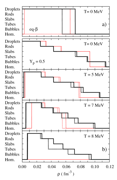
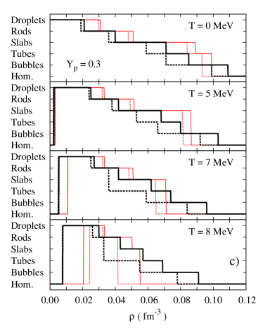
Figure 1: Pasta phases: comparison between NL3 (dashed line) and TW (full line) and the methods CP and TF for a) $\beta$-equilibrium cold stellar matter; b) $Y_{p}=0.5$, c) $Y_{p}=0.3$. The thick lines refer to the Thomas-Fermi (TF) calculation and the thin red lines to the coexisting-phases (CP) calculation.

IV Results and discussions

In the present section we discuss the properties of the pasta phase obtained within the two methods described above. We consider several temperatures, $T=0,5,7,8$ MeV and two proton fractions $Y_{p}=0.5$ and $0.3$. We only show results up to 8 MeV because it is not clear whether our framework model is realistic above this temperature , since thermal fluctuations are not taken into account. The problem of the effect of thermal fluctuations on the pasta structures has been studied by thermal1 ; thermal2 and it was shown that thermally induced displacements of the rod-like and slab-like nuclei can melt the lattice structure when these displacement are larger than the space available between the cluster and the boundary of the Wigner-Seitz cell. While for the rod like clusters $T=8$ MeV would still be acceptable, for the slabs $T=8$ MeV could already be too large.

We perform most of our calculations for a fixed proton fraction, although matter in $\beta$-equilibrium with trapped neutrinos is known to be important. In fact during the first seconds of the protoneutron star, neutrinos are trapped. They start to diffuse out 10-15 s after the supernova explosion burrows86 ; prakash97 , when the fraction of leptons decreases from a maximum value, $\sim$ 0.4, constant through out the star, to smaller values. Neutrino emission is essential to understand neutron star cooling yakovlev01 ; migdal90 . However, neutrinos couple weakly to nuclear matter, therefore for the pasta calculation their presence mainly defines the proton fraction of the warm stellar matter. In ducoin08 , we have shown for a wide set of models, including NL3 and TW, that for the density range of interest for the pasta phase, the proton fraction for the largest trapped fraction of neutrinos, which corresponds to a lepton fraction $Y_{l}\sim 0.4$, is approximately 0.3. Moreover, in a recent paper pasta_alpha we have studied the pasta phase in $\beta$-equilibrium stellar matter with trapped neutrinos ($Y_{l}=0.4$) within the more schematic coexisting phases approach and we have seen that the pasta phase structure and its extension is very similar to the one obtained for a fixed proton fraction of about 0.3.

Since the inclusion of trapped neutrinos in the calculation does not bring much more information about the pasta phase itself (the main point of the present work), we have only included neutrinos in the present calculation for two cases (NL3 and TW, $T=5$ MeV and $Y_{l}=0.4$) in order to show the similarity with the $Y_{p}=0.3$ results.

In Tables 2 and 3 we display the onset densities for each of the pasta structures and the homogeneous phase for the parametrizations NL3 and TW respectively. The pressures identifying the starting ($P^{1}$) and ending ($P^{2}$) points of the pasta phase are also given. We investigate all possible structures for $T=0,5,\,7$ and 8 MeV and proton fraction equal to 0.5 (symmetric matter) and $Y_{p}=0.3$. Both CP and TF approximations were used.

From Table 2 one can observe that TF always presents a richer inner pasta phase structure as compared with the CP method. For $T=8$ MeV and symmetric matter, the pasta phase no longer exists if the CP method is used, but almost all internal structures are present within the TF calculation. Generally, the homogeneous phase becomes the ground-state matter for densities much higher within the TF approach than within the CP method. Just some exceptions were found for a complete structure (3D, 2D, 1D, 2D, 3D) with the TF calculation: $T=7$ MeV for $Y_{p}=0.3$ and $T=8$ MeV for $Y_{p}=0.3$ and $Y_{p}=0.5$, which lack the slab configuration. In all other cases, all possible configurations were found. This is not true within a CP method, where many structures were missing, giving rise to a much simpler pasta phase.

From Table 3 one sees that most of the conclusions drawn for the NL3 parametrization hold true also for TW, as a richer inner pasta phase structure obtained within the TF approach than within the CP method. Once more the homogeneous phase becomes the ground-state matter for densities higher within the TF approach than within the CP method. When the TW density dependent model is used, one can see that all possible internal pasta configurations are always found with the TF approximation. This is not the case with the NL3 parametrization. Different pasta phase internal structures lead to different diffusion coefficients causing different neutrino mean free paths, as seen in opacity . These differences in neutrino opacities may have consequences in calculations of protoneutron star evolution. However, although the internal structures are different as compared with the NL3 parametrization, the densities at which the pasta structure appears and ends are quite similar.

In tables 2 and 3 we have also included the results for $\beta$-equilibrium matter with trapped neutrinos and a lepton fraction $Y_{l}=0.4$ at $T=5$ MeV. It is seen that these results are very similar to the ones obtained for $Y_{p}=0.3$. This is understandable because, for the pasta phase densities, the proton fraction changes from $\sim$ 0.29 for the lowest densities to $\sim 0.32$ for the largest ones. A proton fraction smaller than 0.3 at the onset of the pasta phase explains the onset of the pasta at slightly larger densities. On the other hand a proton fraction $Y_{p}>0.3$ at the upper limit of the pasta phase corresponds in the TF calculation to a slightly larger transition density than the $Y_{p}=0.3$ value, and lies between the value obtained for $Y_{p}=0.5$ and $Y_{p}=0.3$. In the CP calculation the result also lies between $Y_{p}=0.5$ and $Y_{p}=0.3$ but is instead smaller than the $Y_{p}=0.3$ value because CP does not allow for the rearrangement of the proton distribution.

The comparison between Tables 2 and 3 is more easily done analysing Fig. 2. In Fig. 2 we compare the density range for which each pasta configuration exists within NL3 and TW. The thick lines stand for the Thomas-Fermi calculation, the thin ones for the CP method. Full lines represent TW and dahsed ones NL3.

For symmetric matter the main difference is the the appearance of the different phases at slightly smaller densities within NL3. The largest differences occur for $Y_{p}=0.3$: NL3 has no slab phase at T=7 and 8 MeV and quite large tube and bubble phases.

It has been discussed in oyamatsu07 ; watanabe08 that the characteristics of the pasta phase are strongly related with the density dependence of the symmetry energy. In particular, in watanabe08 the pasta phases have been calculated using quantum molecular dynamics. The authors have considered two models, and have obtained a quite different structure for the pasta phase of both models. The slab phase is very small in one of the models and although larger in the other, it is one of the phases that first disappears when the temperature is raised.

A large value of the slope of the symmetry energy $L$ means a smaller symmetry energy at sub-saturation densities. Therefore, since TW has a much smaller symmetry energy slope, $L=55$ MeV for TW and $L=118$ MeV for NL3, at sub-saturation densities its symmetry energy is larger and the neutron gas equation of state has a larger energy. As a consequence, neutrons do not drip so easily, the surface tension is larger and the surface is less diffuse. In Table 1 we have included the value of the surface tension $\sigma$ of TW and NL3 for the proton fractions 0.5 and 0.3. It is seen that TW has a much larger $\sigma$ for $Y_{p}=0.3$ than NL3 which is in accordance with its symmetry energy slope. We may now understand the different properties of the TW pasta: the larger surface energy explains the fact that all the pasta phases extend to larger densities. For non-symmetric matter as for $Y_{p}=0.3$ this effect is even stronger. This explains some of the largest differences between NL3 and TW as pointed out before, namely the fact that NL3 has no slab phase above T=7 MeV. As already noticed in pasta1 ; maru2010 the extension of the pasta phase decreases with the increase of the temperature. This is expected because the surface tension decreases with temperature.

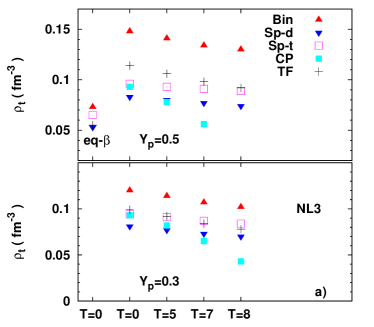
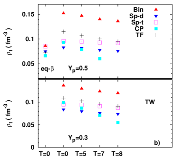
Figure 2: Transition density, for several temperatures $T=0,$ 5, 7 and 8 MeV and proton fractions $Y_{p}=0.5$ (upper plots), $0.3$ (lower plots) and $\beta$-equilibrium (eq-$\beta$) at T=0 (left part of upper plots), obtained using different methods within the models a) NL3 and b) TW. The methods used are: estimation from binodal (Bin), estimation from dynamical spinodal (Sp-d) estimation from thermodynamical spinodal (Sp-th), calculation using the coexisting-phases method (CP) and calculation using a Thomas-Fermi method (TF).

Fig. 2 also allows for a clear comparison between the CP and TF methods: the phases droplets, rods and slabs are stable until larger densities with CP. On the other hand, the phases tubes and bubbles do not appear as the ground-state configuration since they have a higher free energy than the homogeneous matter. Other important differences are the smaller extension of the pasta phase within CP (it starts at larger densities and finishes at smaller densities), and the disappearance of the pasta phase at smaller temperatures. A smaller extension of the pasta phase within the CP method is partially due to non-selfconsistent treatment of the Coulomb interaction maruyama , which prevents the rearrangement of the proton distributions (see also pasta_alpha ). This is more strongly seen for the $Y_{p}=0.5$ when Debye screening effects are stronger. We have calculated the critical temperatures within the CP calculation, above which the pasta phase does not exist. For NL3 we have $T_{c}^{CP}=7.73,\,(8.09)$ MeV for $Y_{p}=0.5,\,(0.3)$, for TW $T_{c}^{CP}=7.95,\,(8.42)$ MeV for $Y_{p}=0.5,\,(0.3)$. The CP critical temperature occurs when the free energy of the homogeneous phase is smaller than the free energy of the pasta phase, and is not defined by a zero surface tension, as in TF. At and above the critical temperature, pasta clusters still exist within CP calculation but with a larger free energy than homogeneous matter.

Finally, it is interesting to compare the prediction of different methods for the crust-core (non-homogeneous–homogeneous) transition density. The thermodynamical binodal and spinodal of proton-neutron $(pn)$ matter give a good estimation of the extension of the pasta phase in nuclear matter. The binodal surface is defined in the $\rho,\,Y_{p},\,T$ space as the surface where the gas and liquid phases coexist and it defines an upper limit for the extension of the pasta phase since it does not take into account neither Coulomb nor finite size effects. The thermodynamical spinodal defines the surface in the $\rho,\,Y_{p},\,T$ space where the curvature of the free-energy of $pn$ matter becomes negative, and gives a rough estimation of the lower limit of the pasta phase extension. Also in this case nor electron effects neither finite range effects are taken into account. The transition density is obtained from the intersection between the $\beta$-equilibrium EoS and the spinodal or binodal surfaces. It is possible to get a better estimation of the lower limit of the pasta phase extension if, instead of the thermodynamical spinodal, the dynamical spinodal is calculated. This surface is defined by the density, proton fraction and temperature for which matter becomes unstable to small density fluctuations and is calculated including electrons, the Coulomb interaction and finite range effects. It has been shown in oyamatsu07 ; pasta1 ; pasta2 ; xu09 that the thermodynamical method gives a good estimation of the transition density for cold $\beta$-equilibrium matter, although a bit too large. For a fixed temperature, the binodal, thermodynamical and dynamical spinodals touch each other (or almost touch) at the critical point muller95 : this corresponds to a quite small proton fraction and is close to the crust-core transition density. However, for less asymmetric matter as the one that occurs in stellar matter with trapped neutrinos, the binodal occurs at quite larger densities than the spinodals. This is clearly seen in Fig. 1 comparing the beta-equilibrium results for cold stellar matter with the results for $Y_{p}=0.5$ or 0.3.

For densities above the binodal surface, matter is homogeneous. For densities below the dynamical spinodal matter is non-homogeneous. Between this two surfaces we may find matter in a metastable configuration. The most probable configuration is the one with the smallest free energy density. The results given in Tables 2 and 3 refer to the energetically favoured configurations. However, we may argue that at finite temperature there may be a coexistence of several configurations with larger or smaller probability according to the corresponding free energy density. This partially justifies the large differences between the TF and CP results: although the ground-state configurations are different, there is not a large energy difference between the configurations and, taking into account an average over all the possible configurations with a correct probability factor would give similar predictions.

In Fig. 1 we compare the transition density from a non-homogeneous phase to a homogeneous phase obtained from the binodal surface muller95 , the dynamical spinodal surface pethick95 ; douchin00 ; providencia06 ; ducoin08 ; ducoin08a ; xu09 , the thermodynamic spinodal surface baoli02 ; avancini06 ; xu09 and from the two methods we have used for the calculation of the pasta phase. As expected the TF result lies always between the results obtained from the dynamical spinodal and the binodal surfaces. This is a self-consistent method that should satisfy these two constraints. This is no longer true for the CP calculation, which, for larger temperatures, fails with predictions that lie below the dynamical spinodal result. It is impressive that the thermodynamical-spinodal result gives so good results when it does not take into account neither the surface nor the Coulomb effects. These are good news because it allows a quite safe prediction from a simple calculation. Finally, it should also be pointed out that for $\beta$-equilibrium matter all methods except CP give similar results. This is due to the occurrence of the transition density close the critical point where the spinodal and binodal surfaces touch and the pressure on these surfaces is maximum.

Table 2: Pasta phases within NL3 for several temperatures and isospin asymmetries. The onset densities of the various phases (droplets, rods, slabs, tubes and bubbles) are shown together with the pressure of the homogeneous phase at the lower ($P^{1}$) and upper ($P^{2}$) border of the pasta phase. The results have been obtained within the coexisting phases method (CP) and the Thomas Fermi approximation (TF).

		onset density (fm-3)						$P^{1}~{}/~{}P^{2}$
	EOS	droplet	rod	slab	tube	bubble	hom	(MeV fm-3)
$T=0$ MeV
$Y_{p}=0.5$
	TF	0.000	0.025	0.043	0.073	0.089	0.114	- / 2.75
	CP	0.000	0.032	0.053	-	-	0.093	- / 1.88
$Y_{p}=0.3$
	TF	0.000	0.019	0.036	0.059	0.071	0.099	- / 1.11
	CP	0.000	0.030	0.048	0.084	-	0.093	- / 0.96
$\beta$-equilibrium
	TF	0.000	-	-	-	-	0.055	- /0.26
	CP	-	-	-	-	-	-	-/-
$T=5$ MeV
$Y_{p}=0.5$
	TF	0.0020	0.026	0.043	0.067	0.081	0.106	0.024$~{}/~{}$2.55
	CP	0.0035	0.031	0.051	-	-	0.078	0.046$~{}/~{}$1.53
$Y_{p}=0.3$
	TF	0.0022	0.024	0.038	0.053	0.066	0.092	0.018$~{}/~{}$1.08
	CP	0.0029	0.032	0.049	0.081	-	0.082	0.025$~{}/~{}$0.85
$Y_{l}=0.4$
	TF	0.0024	0.023	0.036	0.054	0.065	0.093	0.023$~{}/~{}$5.24
	CP	0.0033	0.031	0.049	-	-	0.080	0.024 / 1.43
$T=7$ MeV
$Y_{p}=0.5$
	TF	0.0048	0.026	0.042	0.054	0.072	0.098	0.076$~{}/~{}$2.37
	CP	0.013	0.030	0.049	-	-	0.056	0.22$~{}/~{}$1.06
$Y_{p}=0.3$
	TF	0.0052	0.025	-	0.036	0.059	0.084	0.056$~{}/~{}$1.02
	CP	0.0107	0.032	0.048	-	-	0.065	0.112$~{}/~{}$0.67
$T=8$ MeV
$Y_{p}=0.5$
	TF	0.0069	0.025	-	0.036	0.063	0.092	0.121$~{}/~{}$2.23
	CP	-	-	-	-	-	-	-$~{}/~{}$-
$Y_{p}=0.3$
	TF	0.0076	0.026	-	0.033	0.055	0.078	0.090$~{}/~{}$0.96
	CP	0.0239	0.032	-	-	-	0.043	0.253$~{}/~{}$0.44

Table 3: Pasta phases within TW for several temperatures and isospin asymmetries. The onset densities of the various phases (droplets, rods, slabs, tubes and bubbles) are shown together with the pressure of the homogeneous phase at the lower ($P^{1}$) and upper ($P^{2}$) border of the pasta phase. The results have been obtained within the coexisting phases method (CP) and the Thomas Fermi approximation (TF).

		onset density (fm-3)						$P^{1}~{}/~{}P^{2}$
	EOS	droplet	rod	slab	tube	bubble	hom	(MeV fm-3)
$T=0$ MeV
$Y_{p}=0.5$
	TF	0.000	0.025	0.043	0.075	0.090	0.115	- /2.77
	CP	0.000	0.033	0.054	-	-	0.093	- /1.85
$Y_{p}=0.3$
	TF	0.000	0.021	0.040	0.071	0.085	0.109	-/ 1.22
	CP	0.000	0.031	0.051	0.89	-	0.099	-/ 0.96
$\beta$-equilibrium
	TF	0.000	-	-	-	-	0.073	- / 0.36
	CP	0.003	-	-	-	-	0.066	0.007/ 0.29
$T=5$ MeV
$Y_{p}=0.5$
	TF	0.0022	0.026	0.043	0.071	0.084	0.107	0.027$~{}/~{}$2.53
	CP	0.0038	0.032	0.052	-	-	0.079	0.050$~{}/~{}$1.55
$Y_{p}=0.3$
	TF	0.0024	0.025	0.042	0.068	0.080	0.103	0.020$~{}/~{}$1.20
	CP	0.0032	0.033	0.052	-	-	0.087	0.028$~{}/~{}$0.86
$Y_{l}=0.4$
	TF	0.0026	0.025	0.042	0.068	0.081	0.104	0.026$~{}/~{}$1.64
	CP	0.0035	0.033	0.051	-	-	0.085	0.036$~{}/~{}$1.13
$T=7$ MeV
$Y_{p}=0.5$
	TF	0.0051	0.027	0.043	0.063	0.077	0.100	0.082$~{}/~{}$2.41
	CP	0.0130	0.031	0.051	-	-	0.060	0.225$~{}/~{}$1.16
$Y_{p}=0.3$
	TF	0.0055	0.027	0.042	0.062	0.074	0.096	0.061$~{}/~{}$1.16
	CP	0.0110	0.033	0.051	-	-	0.071	0.120$~{}/~{}$0.72
$T=8$ MeV
$Y_{p}=0.5$
	TF	0.0073	0.027	0.043	0.056	0.072	0.095	0.130$~{}/~{}$2.32
	CP	-	-	-	-	-	-	-$~{}/~{}$-
$Y_{p}=0.3$
	TF	0.0079	0.030	0.043	0.057	0.069	0.091	0.096$~{}/~{}$1.13
	CP	0.0207	0.033	0.050	-	-	0.055	0.234$~{}/~{}$0.57

V Conclusions

In the present work we have calculated the pasta phase at zero and finite temperature applying two different methods already used in previous works: the more naive coexisting-phases method based on the Gibbs construction and the self-consistent Thomas Fermi method. For the first method we need to know the surface tension of the models as a function of temperature and proton fraction. This quantity was parametrized from a Thomas Fermi calculation for semi-infinite nuclear matter pasta_alpha . We had already compared the two models at zero temperature pasta1 ; pasta2 but for the CP calculation we had used a parametrization for the surface tension obtained from Skyrme forces. Since the appearance of the pasta phases has a strong dependence on this quantity the comparison between the models at zero temperature was not conclusive.

We have considered two different relativistic nuclear models: NL3, a parametrization of the NLWM, and TW, a parametrization of the density dependent hadronic model. These two models have quite different behaviors both in the isoscalar and isovector channels. In particular, TW has a quite small slope of the symmetry energy at saturation, $L=$ 55 MeV, while this value is 118 MeV for NL3. The properties of the models are clearly reflected in the pasta phase structure as discussed in watanabe08 .

We conclude that while the CP method allows the determination of the overall trends of both models, it fails at a more detailed and quantitative level. The main trends observed are: the model having a larger surface tension predicts larger density ranges for the pasta phases; the pasta phase extension decreases with temperature; some of the less stable pasta structures may disappear for larger temperatures and/or isospin asymmetries. We have also shown that the overall conclusions obtained within the Thomas Fermi calculation at finite temperature agree with the conclusions obtained from a quantum molecular dynamics calculation watanabe08 . In fact, it was shown that the structure of the pasta is sensitive to the model, namely the density dependence of the symmetry energy. A model with a large symmetry energy slope such as NL3, has a quite small symmetry energy at sub-saturation densities and this favours neutron drip. As a consequence the background neutron gas is larger for NL3 at a given density and therefore, the favoured pasta structures change shape at smaller densities.

We have also compared the crust-core transition density, from a non-homogeneous phase to a homogeneous phase, obtained from the above two methods as well as using other methods often referred to in the literature. It was also shown that the dynamical spinodal defines a lower limit while the binodal a higher limit and the TF result lies between the two limits. The CP methods fails these constraints both for large temperatures, above T=5 MeV, and very asymmetric matter. We have obtained the interesting result that the estimates obtained from a thermodynamical calculation are very close to the prediction of the TF calculation.

Appendix

In this appendix we calculate Eq. (18) for the surface tension $\sigma$, following very closely reference dmcp . The system is composed by $np$ matter and the density depends only upon the $z$ coordinate. Notice that no Coulomb field is included in the calculation of $\sigma$. We start from the grand-canonical potential, Eq. (12), where

$$\Omega=\int\mbox{d}V\left\{\frac{1}{2}\left[(\nabla\phi_{0})^{2}-(\nabla V_{0})^{2}-(\nabla b_{0})^{2}\right]-V_{ef}\right\}$$ (19)

with

$$V_{ef} = -\frac{1}{2}\left[m_{s}^{2}\phi_{0}^{2}+\frac{2}{3!}\kappa\phi_{0}^{3}+\frac{2}{4!}\lambda\phi_{0}^{4}\right.$$ (20)

$$\phantom{mmm}\left.-m_{v}^{2}V_{0}^{2}-m_{\rho}^{2}b_{0}^{2}+2\Sigma_{0}^{R}\rho\right]$$

$$+ 2T\sum_{i=p,n}\int\frac{\mbox{d}^{3}p}{(2\pi)^{3}}\left[\ln(1+e^{-(\epsilon^{*}-\nu_{i})/T})\right.$$

$$+ \left.\ln(1+e^{-(\epsilon^{*}+\nu_{i})/T})\right].$$

The equations of motion for the the meson fields are obtained by minimizing $\Omega$ with respect to each field,

$$\nabla^{2}\phi_{0} = \frac{\mbox{d}^{2}\phi_{0}}{\mbox{d}z^{2}}=-\frac{\partial V_{ef}}{\partial\phi_{0}},$$ (21)

$$\nabla^{2}V_{0} = \frac{\mbox{d}^{2}V_{0}}{\mbox{d}z^{2}}=\frac{\partial V_{ef}}{\partial V_{0}},$$ (22)

$$\nabla^{2}b_{0} = \frac{\mbox{d}^{2}b_{0}}{\mbox{d}z^{2}}=\frac{\partial V_{ef}}{\partial b_{0}}.$$ (23)

Using the relation

$$\frac{\mbox{d}^{2}\,W}{\mbox{d}z^{2}}=\frac{d}{dz}\left(\frac{d\,W}{dz}\right)=\frac{1}{2}\frac{d}{dW}\left(\frac{d\,W}{dz}\right)^{2},$$

where $W=\phi_{0},V_{0},b_{0}$, we obtain

$$\frac{\partial}{\partial\phi_{0}}\left[\frac{1}{2}\left(\frac{d\,\phi_{0}}{dz}\right)^{2}+V_{ef}\right] = 0$$

$$\frac{\partial}{\partial V_{0}}\left[\frac{1}{2}\left(\frac{d\,V_{0}}{dz}\right)^{2}-V_{ef}\right] = 0$$

$$\frac{\partial}{\partial b_{0}}\left[\frac{1}{2}\left(\frac{d\,b_{0}}{dz}\right)^{2}-V_{ef}\right] = 0~{}.$$ (24)

Summing adequately the three equations (the second and third equations multiplied by -1), we get

$$\delta\left[\frac{1}{2}\left(\frac{d\,\phi_{0}}{dz}\right)^{2}-\left(\frac{d\,V_{0}}{dz}\right)^{2}-\left(\frac{d\,b_{0}}{dz}\right)^{2}+V_{ef}\right]=0.$$ (25)

This is equivalent to saying that

$$\frac{1}{2}\left[\left(\frac{d\,\phi_{0}}{dz}\right)^{2}-\left(\frac{d\,V_{0}}{dz}\right)^{2}-\left(\frac{d\,b_{0}}{dz}\right)^{2}\right]+V_{ef}={\cal{C}},$$ (26)

where ${\cal{C}}$ is a constant which corresponds to the bulk contribution to the grand canonical potential density and can be identified with the pressure $P$. Replacing Eq. (26) into (19) we obtain

$$\Omega=\int\mbox{d}V\left[\left(\frac{d\,\phi_{0}}{dz}\right)^{2}-\left(\frac{d\,V_{0}}{dz}\right)^{2}-\left(\frac{d\,b_{0}}{dz}\right)^{2}\right]-{\cal{C}}V.$$ (27)

The surface energy is obtained from the free energy of a system with a fixed number of particles $N=N_{p}+N_{n}$, in which a cluster of arbitrary size exists in the background of the vapor phase. The free energy reads

$$F = \Omega+\mu_{p}N_{p}+\mu_{n}N_{n},$$ (28)

$$= S\int_{-\infty}^{\infty}\mbox{d}z\left[\left(\frac{\mbox{d}\phi_{0}}{\mbox{d}z}\right)^{2}-\left(\frac{\mbox{d}V_{0}}{\mbox{d}z}\right)^{2}-\left(\frac{\mbox{d}b_{0}}{\mbox{d}z}\right)^{2}\right]$$

$$-{\cal{C}}V+\mu_{p}N_{p}+\mu_{n}N_{n}.$$

For a cluster of volume $V$ and surface $S$, we have

$$F=S\sigma-{\cal{C}}V+\mu_{p}N_{p}+\mu_{n}N_{n}.$$ (29)

The surface energy per unit area of this cluster is

$$\sigma=\int_{-\infty}^{\infty}\mbox{d}z\left[\left(\frac{\mbox{d}\phi_{0}}{\mbox{d}z}\right)^{2}-\left(\frac{\mbox{d}V_{0}}{\mbox{d}z}\right)^{2}-\left(\frac{\mbox{d}b_{0}}{\mbox{d}z}\right)^{2}\right].$$ (30)

Eq. (29) can be rewritten in the form of Eq. (3.14) of reference centel

$$\sigma=\int_{-\infty}^{\infty}dz\left[{\cal F}(z)-{\cal F}_{g}-\mu_{p}(\rho_{p}(z)-\rho_{p,g})\right.$$

$$\phantom{mmmmmm}\left.-\mu_{n}(\rho_{n}(z)-\rho_{n,g})\right].$$ (31)

where ${\cal F}_{g}=-P+\mu_{p}\rho_{p,g}+\mu_{n}\rho_{n,g}$, $\rho_{p,g}$ and $\rho_{n,g}$ are the free energy density, the proton density and the neutron density of the gas. We have checked numerically the equivalence between eqs. (30) and (31).

Erratum: Warm pasta phase in the Thomas-Fermi approximation [Phys. Rev. C 82, 055807 (2010)]

Sidney S. Avancini Silvia Chiacchiera Débora P. Menezes Constança Providência

PACS number(s): 21.65.-f, 24.10.Jv, 26.60.-c, 95.30.Tg

There was an error in the numerical code for the CP method that resulted in using the zero temperature surface tension for all the cases, instead of the temperature dependent one. Also, applying the CP method, we found that in the surface energy parametrization given in Ref. pasta_alpha2 the global proton fraction should be used. As a result, the agreement between the more “naïve” CP and the TF calculations has improved. The figures and the table including the correct values for CP are shown below.

In the following, some specific comments we made are corrected. In the CP approximation, the “pasta” phase is found in all the cases considered: the critical temperature for its existence is therefore higher than $8$ MeV. The region in which the “pasta” phase exists is still generally smaller in the CP approach than in the TF one, but some exceptions are found (see Fig. 1). Concerning the transition density (see Fig. 2), the CP results are now much closer to the TF ones. Moreover, for temperatures lower than 7 MeV, they satisfy the constraints imposed by the two spinodals.

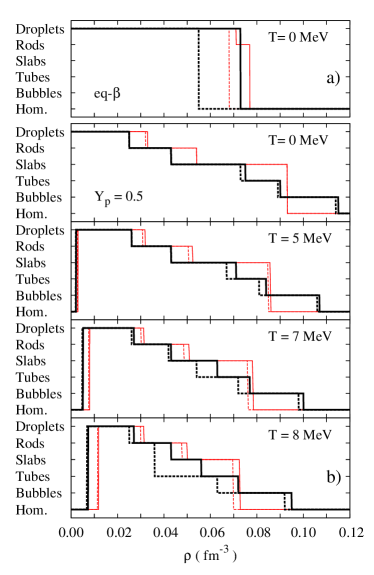
Figure 1: Pasta phases: comparison between NL3 (dashed line) and TW (full line) and the methods CP and TF for a) $\beta$-equilibrium cold stellar matter; b) $Y_{p}=0.5$, c) $Y_{p}=0.3$. The thick lines refer to the Thomas-Fermi (TF) calculation and the thin red lines to the coexisting-phases (CP) calculation.

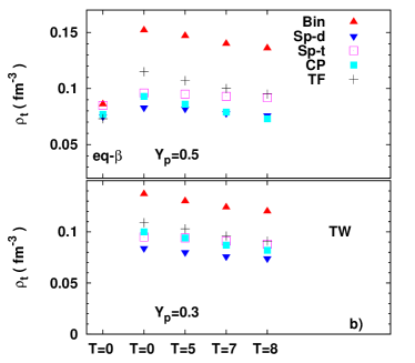
Figure 2: Transition density, for several temperatures $T=0,$ 5, 7 and 8 MeV and proton fractions $Y_{p}=0.5$ (upper plots), $0.3$ (lower plots) and $\beta$-equilibrium (eq-$\beta$) at T=0 (left part of upper plots), obtained using different methods within the models a) NL3 and b) TW. The methods used are: estimation from binodal (Bin), estimation from dynamical spinodal (Sp-d) estimation from thermodynamical spinodal (Sp-th), calculation using the coexisting-phases method (CP) and calculation using a Thomas-Fermi method (TF).

Table 1: Pasta phases within NL3 and TW for several temperatures and isospin asymmetries. The onset densities of the various phases (droplets, rods, slabs, tubes and bubbles) are shown together with the pressure of the homogeneous phase at the lower ($P^{1}$) and upper ($P^{2}$) border of the pasta phase. The results have been obtained within the coexisting-phases method (CP), corrected according to the text explanation, and the Thomas-Fermi approximation (TF), coincident with results in Phys. Rev. C 82, 055807 (except for two misprints for $P^{2}$ at $T=5$ MeV and with $Y_{l}=0.4$).

	EOS	NL3								TW
		Onset density (fm-3)						$P^{1}~{}/~{}P^{2}$		Onset density (fm-3)						$P^{1}~{}/~{}P^{2}$
		droplet	rod	slab	tube	bubble	hom	(MeV/fm3)		droplet	rod	slab	tube	bubble	hom	(MeV/fm3)
$T=0$ MeV
$Y_{p}=0.5$	TF	0.000	0.025	0.043	0.073	0.089	0.114	- / 2.75		0.000	0.025	0.043	0.075	0.090	0.115	- / 2.77
$Y_{p}=0.5$	CP	0.000	0.032	0.054	-	-	0.093	- / 1.88		0.000	0.033	0.054	-	-	0.093	- / 1.85
$Y_{p}=0.3$	TF	0.000	0.019	0.036	0.059	0.071	0.099	- / 1.11		0.000	0.021	0.040	0.071	0.085	0.109	- / 1.22
$Y_{p}=0.3$	CP	0.000	0.030	0.048	0.085	-	0.097	- / 0.96		0.000	0.031	0.051	0.089	-	0.100	- / 0.96
$\beta$-equil.	TF	0.000	-	-	-	-	0.055	- / 0.26		0.000	-	-	-	-	0.073	- / 0.36
$\beta$-equil.	CP	0.000	-	-	-	-	0.068	- / 0.49		0.000	0.071	-	-	-	0.077	- / 0.41
$T=5$ MeV
$Y_{p}=0.5$	TF	0.0020	0.026	0.043	0.067	0.081	0.106	0.024 / 2.55		0.0022	0.026	0.043	0.071	0.084	0.107	0.027 / 2.53
$Y_{p}=0.5$	CP	0.0028	0.031	0.051	-	-	0.085	0.035 / 1.76		0.0030	0.032	0.052	-	-	0.086	0.039 / 1.76
$Y_{p}=0.3$	TF	0.0022	0.024	0.038	0.053	0.066	0.092	0.018 / 1.08		0.0024	0.025	0.042	0.068	0.080	0.103	0.020 / 1.20
$Y_{p}=0.3$	CP	0.0009	0.032	0.049	0.081	-	0.091	0.007 / 1.06		0.0015	0.033	0.052	0.088	-	0.094	0.012 / 1.01
$Y_{l}=0.4$	TF	0.0024	0.023	0.036	0.054	0.065	0.093	0.023 / 1.38		0.0026	0.025	0.042	0.068	0.081	0.104	0.026 / 1.64
$Y_{l}=0.4$	CP	0.0011	0.031	0.049	0.082	-	0.090	0.009 / 1.36		0.0019	0.033	0.052	0.089	-	0.092	0.018 / 1.30
$T=7$ MeV
$Y_{p}=0.5$	TF	0.0048	0.026	0.042	0.054	0.072	0.098	0.076 / 2.37		0.0051	0.027	0.043	0.063	0.077	0.100	0.082 / 2.41
$Y_{p}=0.5$	CP	0.0076	0.030	0.049	-	-	0.076	0.124 / 1.62		0.0081	0.031	0.051	-	-	0.079	0.135 / 1.65
$Y_{p}=0.3$	TF	0.0052	0.025	-	0.036	0.059	0.084	0.056 / 1.02		0.0055	0.027	0.042	0.062	0.074	0.096	0.061 / 1.16
$Y_{p}=0.3$	CP	0.0030	0.032	0.048	0.078	-	0.084	0.032 / 1.02		0.0046	0.033	0.051	0.085	-	0.087	0.051 / 0.99
$T=8$ MeV
$Y_{p}=0.5$	TF	0.0069	0.025	-	0.036	0.063	0.092	0.121 / 2.23		0.0073	0.027	0.043	0.056	0.072	0.095	0.130 / 2.32
$Y_{p}=0.5$	CP	0.0114	0.030	0.048	-	-	0.070	0.205 / 1.50		0.0119	0.031	0.050	-	-	0.073	0.217 / 1.56
$Y_{p}=0.3$	TF	0.0076	0.026	-	0.033	0.055	0.078	0.090 / 0.96		0.0079	0.030	0.043	0.057	0.069	0.091	0.096 / 1.13
$Y_{p}=0.3$	CP	0.0047	0.032	0.048	0.075	-	0.079	0.056 / 0.99		0.0070	0.033	0.050	-	-	0.082	0.085 / 0.97

References

- (1) D. G. Ravenhall, C.J. Pethick and J.R. Wilson, Phys. Rev. Lett. 50, 2066 (1983).
- (2) C.J. Horowitz, M.A. Pérez-Garcia and J. Piekarewicz, Phys. Rev. C 69, 045804 (2004); C.J. Horowitz, M.A. Pérez-Garcia, D.K. Berry and J. Piekarewicz, Phys. Rev. C 72, 035801 (2005).
- (3) T. Maruyama, T. Tatsumi, D.N. Voskresensky, T. Tanigawa and S. Chiba, Phys. Rev. C 72, 015802 (2005).
- (4) Gentaro Watanabe, Toshiki Maruyama, Katsuhiko Sato, Kenji Yasuoka, and Toshikazu Ebisuzaki, Phys. Rev. Lett. 94, 031101 (2005).
- (5) Hidetaka Sonoda, Gentaro Watanabe, Katsuhiko Sato, Kenji Yasuoka, and Toshikazu Ebisuzaki, Phys. Rev. C 77, 035806 (2008); ibid, Phys. Rev. C 81, 049902 (2010).
- (6) S.S. Avancini, D.P. Menezes, M.D. Alloy, J.R. Marinelli, M.M.W. Moraes and C. Providência, Phys. Rev. C 78, 015802 (2008).
- (7) J. Xu, L.W. Chen, B.A. Li and H.R. Ma, Phys. Rev. C 79, 035802 (2009).
- (8) S.S. Avancini, L. Brito, J.R. Marinelli, D.P. Menezes, M.M.W. de Moraes, C. Providência and A.M. Santos - Phys. Rev. C 79, 035804 (2009).
- (9) G. A. Lalazissis, J. König and P. Ring, Phys. Rev. C 55, 540 (1997).
- (10) S. Typel and H. H. Wolter, Nucl. Phys. A656, 331 (1999); Guo Hua, Liu Bo and M. Di Toro, Phys. Rev. C 62, 035203(2000).
- (11) T. Klähn et al., Phys. Rev. C 74, 035802 (2006).
- (12) L.W.Chen, C. M. Ko, and B. A. Li, Phys. Rev. Lett. 94, 032701 (2005); Phys. Rev. C 72, 064309 (2005).
- (13) P. Gögelein, E.N.E. van Dalen, C. Fuchs and H. Müther, Phys. Rev. C 77, 025802 (2008).
- (14) E.N.E. van Dalen, C. Fuchs and A. Faessler, Eur. Phys. J.A. 31, 29(2007).
- (15) S.S. Avancini, C.C. Barros, D.P. Menezes and C. Providência, Phys. Rev. C 82, 025808 (2010).
- (16) M.D. Alloy and D.P. Menezes, arXiv:1011.0968 [nucl-th].
- (17) S. S Avancini et al. Int. J. Mod. Phys. D 19, 1587 (2010).
- (18) Toshiki Maruyama, Toshitaka Tatsumi, arXiv:1009.1198v1 [nucl-th].
- (19) Bennett Link, Richard I. Epstein, and James M. Lattimer, Phys. Rev. Lett. 83, 3362 (1999).
- (20) C. J. Pethick, D. G. Ravenhall, and C. P. Lorenz, Nucl. Phys. A 584, 675 (1995).
- (21) B. A. Li, L. W. Chen, C. M. Ko, Phys. Rep. 464, 113 (2008); J. Xu et al, Astrophys. J. 697, 1549 (2009).
- (22) Kazuhiro Oyamatsu and Kei Iida, Phys. Rev. C 75, 015801 (2007).
- (23) C. Ducoin, C. Providência, A. M. Santos, L. Brito, and Ph. Chomaz, Phys. Rev. C 78, 055801 (2008).
- (24) T. Gaitanos, M. Di Toro, S. Typel, V. Baran, C. Fuchs, V. Greco and H. H. Wolter, Nucl. Phys. A 732, 24 (2004).
- (25) S.S. Avancini, L. Brito, D. P. Menezes and C. Providência, Phys. Rev. C 70, 015203 (2004).
- (26) P. Ring and P. Schuck, The nuclear many-body problem, Springer-Verlag, 1980.
- (27) M. Centelles, X. Viñas and M. Barranco, Ann. Phys. 221 165 (1993).
- (28) Y.K. Gambhir, P. Ring and A. Thimet, Ann. Phys. 198, 132 (1990).
- (29) J. M. Aparicio, Astrophys. J. Suppl. Ser. 117, 627 (1998).
- (30) M. Nielsen and J. da Providência, J. Phys. G: Nucl. Part. Phys. 16, 649 (1990).
- (31) C. Providência, L. Brito and J. da Providência, M. Nielsen and X. Viñas, Phys. Rev. C 54, 2525 (1996).
- (32) D. P. Menezes and C. Providência, Phys. Rev. C 60, 024313 (1999).
- (33) M. Centelles, M. Del Estal and X. Viñas, Nucl. Phys. A 635, 193 (1998).
- (34) D.N. Voskresensky, M. Yasuhira and T. Tatsumi, Phys. Lett. B 541, 93 (2002); Nucl. Phys. A 723 291 (2003).
- (35) N. Yasutake and K. Kashiwa, Phys. Rev. D 79, 043012 (2009).
- (36) T. Maruyama, N. Yasutake and T. Tatsumi, arXiv:1009.1196v1 [nucl-th].
- (37) T. Maruyama, S. Chiba, H. J. Schulze, T. Tatsumi, Phys. Rev. D 76 (2007) 123015.
- (38) C. J. Pethick and A. Y. Potekhin, Phys. Lett. B 427, 7 (1998).
- (39) G. Watanabe, K. Iida and K. Sato, Nucl. Phys. A 676, 455 (2000); Nucl. Phys. A 726, 357 (2003) .
- (40) A. Burrows and J. M. Lattimer, Astrophys. J. 307, 178 (1986).
- (41) M. Prakash, I. Bombaci, M. Prakash, P. J. Ellis, J. M. Lattimer, and R. Knorren, Phys. Rep. 280, 1 (1997).
- (42) G. D. Yakovlev, A. D. Kaminker, O. Y. Gnedin, and P. Haensel, Phys. Rep. 354, 1 (2001).
- (43) A. B. Migdal, E.E. Saperstein, M.A. Troitsky, D.N. Voskresensky, Phys. Rep. 192, 179 (1990).
- (44) H. Müller and B. D. Serot, Phys. Rev. C 52, 2072 (1995).
- (45) F. Douchin and P. Haensel, Phys. Lett. B 485, 107 (2000).
- (46) C. Providência, L. Brito, S. S. Avancini, D. P. Menezes, and Ph. Chomaz, Phys. Rev. C 73, 025805 (2006); L. Brito, C. Providência, A. M. Santos, S. S. Avancini, D. P. Menezes, and Ph. Chomaz, Phys. Rev. C 74, 045801 (2006); H. Pais, A. Santos, L. Brito, and C. Providência, Phys. Rev. C 82, 025801 (2010).
- (47) C. Ducoin, J. Margueron, and P. Chomaz, Nucl. Phys. A 809, 30 (2008).
- (48) B.-A. Li, A. T. Sustich, M. Tilley, and B. Zhang, Nucl. Phys. A 699, 493 (2002).
- (49) S. S. Avancini, L. Brito, D. P. Menezes, and C. Providência Phys. Rev. C 70, 015203 (2004); S. S. Avancini, L. Brito, Ph. Chomaz, D. P. Menezes, and C. Providência, Phys. Rev. C 74, 024317 (2006).

References

- (1) S.S. Avancini, C.C. Barros, D.P. Menezes and C. Providência, Phys. Rev. C 82, 025808 (2010).