Spin dynamics in the XY model

Abstract

We study the evolution of entanglement, quantum correlation and classical correlation for the one dimensional XY model in external transverse magnetic field. The system is initialized in the full polarized state along the z axis, after annealing, different sites will become entangled. We study the three kinds of correlation for both the nearest and the next-nearest neighbor sites. We find that for large anisotropy parameter the quantum phase transition can be indicated by the dynamics of classical correlation between the nearest neighbor sites. We find that the dynamics of entanglement for both the nearest and next-nearest neighbor sites show significantly different behaviors with different values of magnetic field. We also find that the evolution of quantum correlation and classical correlation of the nearest neighbor sites are obviously different from those of the next-nearest neighbor sites.

As an ideal model used to describing phase transition on the early days in statistical mechanics, the XY model has been studied intensely for almost one century. Although it is so simple that it can be calculated analytically, it catches the most important elements of some physical system, such as materials $\textmd{Cs}(\textmd{H}_{1-x}\textmd{D}_{x})_{2}\textmd{PO}_{4}$, $\textmd{PbH}_{1-x}\textmd{D}_{x}\textmd{PO}_{4}$ OD00 , etc. So it could be used to depict the actual phase transition very well. It also became the test bed equipped to describe more practice physical system, and to examine the performance of different approximation methods E70 . With the birth of quantum information theory, it was found that the XY model could be used as a quantum information channel. So it became the focus of theoretical and experimental studying again Do07 , and many quantum information process has been proposed with the XY model C04 ; A04 ; W07 .

There were many works on quantum information process in the XY and the Ising model, such as the transfer of an unknown quantum state along the chain C04 ; A04 ; B06 . As an important resource in quantum information process, it was found that entanglement could be used as an quantity to indicate quantum phase transition AO02 ; O02 . Recently, it has been reported that dynamics of the nearest-neighbor entanglement may be used as an indicator of quantum phase transition in the transverse Ising model Zhe10 . In fact, quantum entanglement is only a special part of the quantum correlation H02 ; Ve03 ; J09 ; Ka10 , there is other quantum correlation that is not caught by the quantum entanglement, and it is found to be important in quantum information task Me00 ; L08 ; Da08 . More correlation indicates more information, so it is not trivial to study the evolution of the quantum correlation.

In this paper, we study the entanglement, quantum correlation and classical correlation dynamics of both the nearest and next-nearest neighbor sites in the one dimensional transverse XY model with the initial state been the full polarized state along the z axis. For different values of anisotropy parameter, we find that the entanglement takes on distinctive behaviors with different values of magnetic field. We find that for large value of anisotropy parameter the first maximum of classical correlation between the nearest neighbor sites peaks around the critical point. That may be an indicator of quantum phase transition. Further more, we find that behaviors of the three kinds of correlation for the nearest neighbor sites are obviously different from those for the next-nearest neighbor sites.

The Hamiltonian of the one dimensional XY model in transverse magnetic field reads as

$$H=-\lambda\sum_{i=1}^{N}[(1+\gamma)S_{i}^{x}S_{i+1}^{x}+(1-\gamma)S_{i}^{y}S_{i+1}^{y}]-\sum_{i=1}^{N}S_{i}^{z},$$ (1)

where $S_{i}^{\alpha}$ $(\alpha=x,y,z)$ are the spin $1/2$ matrixes at site $i$, and $N$ is the number of sites. We assume periodic boundary conditions $S_{i}^{\alpha}=S_{N+i}^{\alpha}$, and the anisotropy parameter $\gamma$ divides the whole parameter space into two classes, for $\gamma=0$, it is the XX model, and $0<\gamma\leq 1$ belongs to the Ising universality class. Here we will only concentrate on the thermodynamic limit $N=\infty$, at which the Hamiltonian system undergoes a quantum phase transition at $\lambda_{c}=1$.

This model could be solved analytically by mapping the spin half system into the spinless fermion system via the Jordan-Wigner transformation E70

$$S_{j}^{x} = \frac{1}{2}(b^{\dagger}_{j}exp(i\pi\sum_{k=1}b^{\dagger}_{k}b_{k})+exp(-i\pi\sum_{k=1}b^{\dagger}_{k}b_{k})b_{j}),$$

$$S_{j}^{y} = \frac{1}{2i}(b^{\dagger}_{j}exp(i\pi\sum_{k=1}b^{\dagger}_{k}b_{k})-exp(-i\pi\sum_{k=1}b^{\dagger}_{k}b_{k})b_{j}),$$

$$S_{j}^{z} = b^{\dagger}_{j}b_{j}-\frac{1}{2},$$ (2)

where $b_{j}^{\dagger}$ ($b_{j}$) is the creation (annihilation) operator of the spinless fermion. After application of the Fourier and Bogoliubov transformation $\eta=\frac{1}{\sqrt{N}}\sum_{l}e^{ikl}(\alpha_{k}b_{l}+i\beta_{k}b^{\dagger}_{l})$, with parameters $\alpha_{k}=\frac{\Lambda_{k}-(1+\lambda\textsf{cos}k)}{\sqrt{2[\Lambda_{k}^{2}-(1+\lambda\textsf{cos}k)\Lambda_{k}]}}$, $\beta_{k}=\frac{\gamma\lambda\textsf{sin}k}{\sqrt{2[\Lambda_{k}^{2}-(1+\lambda\textsf{cos}k)\Lambda_{k}]}}$, the eventually Hamiltonian can be diagonalized as

$$H=\sum_{k}\Lambda_{k}(\eta^{\dagger}_{k}\eta_{k}-\frac{1}{2}),$$ (3)

with the eigenenergy spectrum $\Lambda_{k}=\sqrt{(1+\lambda\textsf{cos}k)^{2}+\lambda^{2}\gamma^{2}\textsf{sin}^{2}k}$.

The time evolution of the spin system in Eq. (1), can be given by the evolution of the spinless fermion operator $b_{j}(t)$ La04

$$b_{j}(t)=\frac{1}{N}\sum_{k,l}[\textsf{cos}k(l-j)c_{k}(t)b_{l}-2i\textsf{sin}k(l-j)d_{k}(t)b^{\dagger}_{l}],$$ (4)

with time dependent coefficients $c_{k}(t)=e^{i\Lambda_{k}t}-2i\beta^{2}_{k}\textsf{sin}\Lambda_{k}t$, $d_{k}(t)=\alpha_{k}\beta_{k}\textsf{sin}\Lambda_{k}t$.

We choose the initial state that all spins are polarized along the $z$ axis, $\rho(0)=|N\rangle\langle N|$, with $|N\rangle=|\uparrow\rangle_{1}...|\uparrow\rangle_{N}$, which is ground state of Eq. (1) when a strong magnetic field is applied along the $z$ axis. Hence, there is no quantum correlation and classical correlation among any partition of the system. Due to the translational symmetry of the system, we choose site 1 as our first site when we study the correlation between different sites. In order to obtain the evolution of entanglement, quantum correlation and classical correlation, we need to get the reduced density matrix first. So we will have to calculate two-body spin correlation functions, it is equal to calculate the fermion correlation function $\langle b_{1}...\rangle_{t}=\langle b_{1}(t)...\rangle_{0}$. From Wick theorem, we can learn that the correlation function will be nonzero for only even number of creation and annihilation operators.

For the first two spins the reduced density matrix in the basis of $|\uparrow\uparrow\rangle,|\uparrow\downarrow\rangle,|\downarrow\uparrow\rangle,|\downarrow\downarrow\rangle,$ is given by

$$\rho^{12}(t)=\begin{pmatrix}\rho^{12}_{11}&0&0&\rho^{12}_{14}\\ 0&\rho^{12}_{22}&\rho^{12}_{23}&0\\ 0&\rho^{12}_{32}&\rho^{12}_{33}&0\\ \rho^{12}_{41}&0&0&\rho^{12}_{44}\end{pmatrix},$$ (5)

where Zhe10

$$\rho^{12}_{11} = \langle b_{1}^{\dagger}(t)b_{1}(t)b_{2}^{\dagger}(t)b_{2}(t)\rangle_{0}=\langle b_{1}^{\dagger}(t)b_{1}(t)\rangle_{0}\langle b_{2}^{\dagger}(t)b_{2}(t)\rangle_{0}$$

$$- \langle b_{1}^{\dagger}(t)b_{2}^{\dagger}(t)\rangle_{0}\langle b_{1}(t)b_{2}(t)\rangle_{0}+\langle b_{1}^{\dagger}(t)b_{2}(t)\rangle_{0}$$

$$\times \langle b_{1}(t)b_{2}^{\dagger}(t)\rangle_{0},$$

$$\rho^{12}_{22} = \rho^{12}_{33}=\langle b_{1}^{\dagger}(t)b_{1}(t)b_{2}(t)b_{2}^{\dagger}(t)\rangle_{0}=\langle b_{1}^{\dagger}(t)b_{1}(t)\rangle_{0}-\rho^{12}_{11},$$

$$\rho^{12}_{44} = \langle b_{1}(t)b_{1}^{\dagger}(t)b_{2}(t)b_{1}^{\dagger}(t)\rangle_{0}=1-\rho^{12}_{11}-2\rho^{12}_{22},$$

$$\rho^{12}_{41} = \rho^{12*}_{14}=\langle b_{1}^{\dagger}(t)b_{2}^{\dagger}(t)\rangle_{0},$$

$$\rho^{12}_{23} = \rho^{12*}_{32}=-\langle b_{1}(t)b_{2}^{\dagger}(t)\rangle_{0}.$$ (6)

At the thermodynamic limit $N=\infty$, we get the following analytical formulations,

$$\langle b_{1}^{\dagger}(t)b_{1}(t)\rangle_{0} = \frac{1}{2\pi}\int_{-\pi}^{\pi}(1-4\alpha_{k}^{2}\beta_{k}^{2}\textsf{sin}^{2}\Lambda_{k}t)dk,$$

$$\langle b_{1}^{\dagger}(t)b_{2}(t)\rangle_{0} = \frac{1}{2\pi}\int_{-\pi}^{\pi}\textsf{cos}k(1-4\alpha_{k}^{2}\beta_{k}^{2}\textsf{sin}^{2}\Lambda_{k}t)dk,$$

$$\langle b_{1}(t)b_{2}(t)\rangle_{0} = \frac{1}{2\pi}\int_{-\pi}^{\pi}\textsf{sin}k\alpha_{k}\beta_{k}(2\textsf{sin}^{2}\Lambda_{k}t(1-2\beta_{k}^{2})$$ (7)

$$- i\textsf{sin}2\Lambda_{k}t)dk.$$

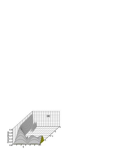
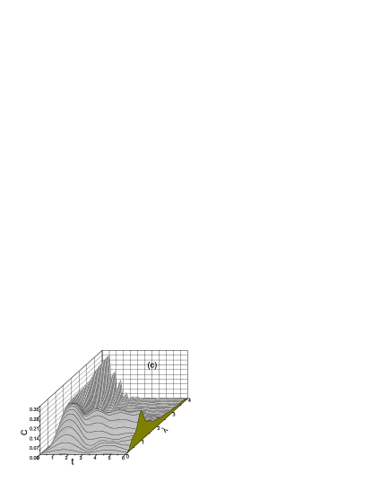
Figure 1: Evolution of (a) entanglement, (b) quantum correlation and (c) classical correlation for the nearest sites, with anisotropy parameter $\gamma=1.0$.

We use concurrence Wo98 to measure the bipartite entanglement. When the density matrix is the ”X” type, it is given by Yu07 $2\textsf{max}[0,|\rho^{12}_{23}|-\sqrt{\rho^{12}_{11}\rho^{12}_{44}},|\rho^{12}_{14}|-\sqrt{\rho^{12}_{22}\rho^{12}_{33}}]$. In order to obtain the dynamics of quantum correlation and classical correlation, we choose quantum discord H02 to measure the quantum correlation (it equals to the quantum correlation H01 in the case of two qubits J09 ; H01 ; Ge10 ). It is given by the discrepancy of two kinds of quantum mutual information derived from their classical counterparts, $D(\rho_{12})=I(\rho_{12})-C(\rho_{12})$, where $C(\rho_{12})=\textsf{max}_{\{\Pi_{j}^{2}\}}(S(\rho_{1})-\sum_{j}q_{j}S(\rho_{1}^{j}))$. $\{\Pi_{j}^{2}\}$ are the complete projective measurement on partition 2, and $q_{j}=\textsf{tr}_{1,2}(\Pi_{j}^{2}\rho_{12})$. $\rho_{1}^{j}=(\Pi_{j}^{2}\rho_{12}\Pi_{j}^{2})/q_{j}$ is the state of partition 1 after partition 2 recording the outcome $j$.

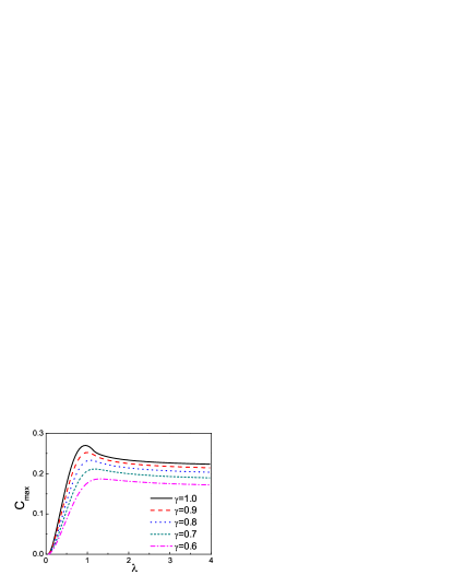
Figure 2: (Color online) The first local maximum of classical correlation for different values of anisotropy parameter. The solid black, dash red, dot blue, short dash dark cyan line denote $\gamma=1.0,0.9,0.8,0.7$ respectively.

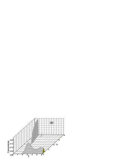
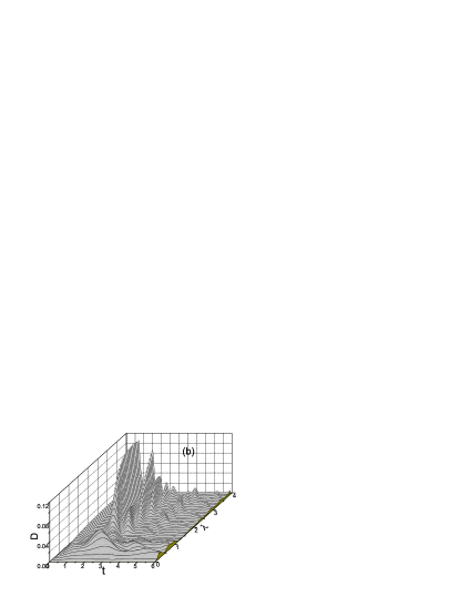
Figure 3: The evolution of (a) entanglement, (b) quantum correlation and (c) classical correlation for the next-nearest neighbor sites with anisotropy parameter $\gamma=1.0$.

The initial state of the spin 1 and spin 2 reads

$$\rho_{12}=\begin{pmatrix}1&0&0&0\\ 0&0&0&0\\ 0&0&0&0\\ 0&0&0&0\\ \end{pmatrix},$$ (8)

so there are neither classical correlation nor quantum correlation between 1 and 2. As the magnetic field quenched ($\lambda$ changes suddenly from zero to a finite value), the initial state will evolve under the XY exchange interaction. In Figure 1(a), (b) and (C), evolution of entanglement, classical correlation and quantum correlation have been shown with the anisotropy parameter $\gamma=1.0$. The behavior of entanglement is complex. There is a definite boundary around $\lambda_{b}\sim 0.86$, when $\lambda\leq\lambda_{b}$ entanglement is present in a long time interval, but when $\lambda\geq\lambda_{b}$ entanglement disappears fast and absents for a longtime. However, the quantum correlation is nonzero almost all the time. So it is clear that it is due to the dissonance Ka10 , another kind of quantum correlation, the quantum correlation could be nonzero without entanglement. From the evolution of both entanglement and quantum correlation we could see that when the magnetic field is large ($\frac{1}{\lambda}$), there will be entanglement all the time. While for a little magnetic field, the dissonance, will be the dominant component of quantum correlation and evolves with time. The classical correlation behaves much the same like the quantum correlation, as the magnetic field decreases classical correlation oscillates much faster, it can be understood as the magnetic field decreases the flipping interaction dominates over the on site potential energy. It can be seen that for all kinds of correlation, they disappear gradually as the magnetic field dying out. This is due to the fact the exchange interaction tend to dispose the nearest sites in the sparable state $(|\uparrow\rangle_{1}+|\downarrow\rangle_{1})\otimes(|\uparrow\rangle_{2}-|\downarrow\rangle_{2})$ or $(|\uparrow\rangle_{1}-|\downarrow\rangle_{1})\otimes(|\uparrow\rangle_{2}+|\downarrow\rangle_{2})$.

For different values of the magnetic field, entanglement, quantum correlation and classical correlation evolve with time, and they will obtain their first local maximum with different values. Particularly, we find that for the classical correlation, its first local maximum $C_{max}$ has a maximum around the critical point $\lambda_{c}=1$. This may be seen as an indicator of the quantum phase transition at the critical point. In fact we find that when the anisotropy parameter is big enough, $\gamma\geq 0.7$, $C_{max}$ always has a maximum around the critical point, as shown in Fig. 2. But as the anisotropy parameter decreases, the maximum gets away from the critical point.

For the next-nearest neighbor sites, we only need to focus on sites 1 and 3. The reduced density matrix takes on the same shape as that of sites 1 and 2, with 3 instead of 2 for the diagonal elements, and the non-diagonal elements are given by

$$\rho^{13}_{23} = \rho^{13*}_{32}=-\langle b_{1}(t)b_{3}^{\dagger}(t)\rangle_{0}+2(\langle b_{1}(t)b_{3}^{\dagger}(t)\rangle_{0}\langle b_{1}^{\dagger}(t)b_{1}(t)\rangle_{0}$$

$$+ \langle b_{1}(t)b_{2}^{\dagger}(t)\rangle_{0}+|\langle b_{1}(t)b_{2}(t)\rangle_{0}|^{2}),$$

$$\rho^{13}_{14} = \rho^{13*}_{41}=-\langle b_{1}(t)b_{3}(t)\rangle_{0}+2(\langle b_{1}(t)b_{3}(t)\rangle_{0}\langle b_{1}^{\dagger}(t)b_{1}(t)\rangle_{0}$$ (9)

$$+ 2Re(\langle b_{1}(t)b_{2}^{\dagger}(t)\rangle_{0})\langle b_{1}(t)b_{2}(t)\rangle_{0},$$

where the transverse symmetry has been used, and $Re$ means the real part of the number. The correspondent correlation functions are

$$\langle b_{1}^{\dagger}(t)b_{3}(t)\rangle_{0} = \frac{1}{2\pi}\int_{-\pi}^{\pi}\textsf{cos}2k(1-4\alpha_{k}^{2}\beta_{k}^{2}\textsf{sin}^{2}\Lambda_{k}t)dk,$$

$$\langle b_{1}(t)b_{3}(t)\rangle_{0} = \frac{1}{2\pi}\int_{-\pi}^{\pi}\textsf{sin}2k\alpha_{k}\beta_{k}(2\textsf{sin}^{2}\Lambda_{k}t(1-2\beta_{k}^{2})$$ (10)

$$-i\textsf{sin}2\Lambda_{k}t)dk.$$

Here for sites 1 and 3 the initial state is also represented by Eq. (7), the dynamics of entanglement is obviously different from that of nearest neighbor sites, for large anisotropy parameter the entanglement does not appear until after a finite time interval, as shown in Fig. 3(a). This is a little counterintuitive, because entanglement between sites 1 (2) and 2 (3) comes into being almost instantly due to their direct interaction. Therefore, it is reasonable for the entanglement between sites 1 and 3 increases from zero once sites 1(2) and 2(3) are entangled. At the same time, there is a small band of $\lambda$ depending on the anisotropy parameter, in which no entanglement will be generated. What is more, for both classical correlation and quantum correlation, far away from the critical point, they become larger as the magnetic field diminishes, as shown in Figures 3(b), 3(c). This is a little unbelievable at the first glance, and is obviously different from the case of the nearest neighbor sites. At this case we do not find that the dynamics of entanglement, quantum discord and classical correlation could be used as indicator of the quantum phase transition at the critical point like the nearest neighbor sites.

In this paper, we have studied the dynamics of entanglement, quantum correlation and classical correlation with one dimensional transverse XY model for both the nearest and next-nearest neighbor sites. We found that for the nearest neighbor sites, when the magnetic field is strong, all three kinds of correlation are larger than those with a weak field. While for the next-nearest neighbor sites, the dynamics is obviously different. For the nearest neighbor sites, two kinds of dynamics are shown with different values of the magnetic field, while for the next-nearest one, there is a narrow band of $\lambda$, in which there is no entanglement generated. What is more, we found that for the nearest neighbor sites, the first maximum $C_{max}$ of classical correlation peaks around the critical point for large anisotropy parameter, it may be used as an indicator of quantum phase transition.

This work was supported by the National Fundamental Research Program, National Natural Science Foundation of China (Grant Nos. 60921091 and 10874162). We thank H. Wichterich for helpful comments and correspondence.

References

- (1) O. Derzhko, T. Krokhmalskii and J. Stolze, J. Phys. A: Math. Gen. 33, 3063 (2000).
- (2) E. Barouch, B.M. McCoy, and M. Dresden, Phys. Rev. A. 2, 1075 (1970); E. Barouch and B.M. McCoy, ibid. 3, 786 (1971).
- (3) S. I. Doronin, E. B. Fel’dman and A. N. Pyrkov, JETP Lett. 85, 519 (2007); F. Iglói and I. Peschel, Europhys. Lett. 89, 40001 (2010).
- (4) M. Christandl, N. Datta, A. Ekert and A. J. Landahl, Phys. Rev. Lett. 92, 187902 (2004).
- (5) C. Albanese, M. Christandl, N. Datta and A. Ekert, Phys. Rev. Lett. 93, 230502 (2004).
- (6) H. Wichterich and S. Bose, Phys. Rev. A. 79, 060302(R) (2009).
- (7) D. Burgarth and S. Bose, Phys. Rev. A. 73, 062321 (2006).
- (8) A. Osterloh, L. Amico, G. Falci, and R. Fazio, Nature (London) 416, 608 (2002).
- (9) T. J. Osborne and M. A. Nielsen, Phys. Rev. A. 66, 032110 (2002).
- (10) Z. Chang and N. Wu, Phys. Rev. A. 81, 022312 (2010).
- (11) H. Ollivier and W. H. Zurek, Phys. Rev. Lett. 88, 017901 (2001).
- (12) V. Vedral, Phys. Rev. Lett. 90, 050401 (2003).
- (13) K. Modi, T. Paterek, W. Son, V. Vedral and M. Williamson, Phys. Rev. Lett. 104, 080501 (2010).
- (14) J. Maziero, L. C. Celeri, R. M. Serra and V. Vedral, Phys. Rev. A. 80, 044102 (2009).
- (15) D. A. Meyer, Phys. Rev. Lett. 85, 2014 (2000).
- (16) B. P. Lanyon, M. Barbieri, M. P. Almeida and A. G. White, Phys. Rev. Lett. 101, 200501 (2008).
- (17) A. Datta, A. Shaji and C. M. Caves, Phys. Rev. Lett. 100, 050502 (2008).
- (18) L. Amico, A. Osterloh, F. Plastina, R. Fazio and G. M. Palma, Phys. Rev. A. 69, 022304 (2004).
- (19) W. K. Wootters, Phys. Rev. Lett. 80, 2245 (1998); S. Hill and W. K. Wootters, ibid. 78, 5022 (1997).
- (20) T. Yu and J. H. Eberly, Quantum information and computation. 7, 459 (2007).
- (21) L. Henderson and V. Vedral, J. Phys. A. 34, 6899 (2001).
- (22) R.-C. Ge, M. Gong, C.-F. Li, J.-S. Xu and G.-C. Guo, Phys. Rev. A. 81, 064103 (2010).