Photocurrent in a visible-light graphene photodiode

Abstract

We calculate the photocurrent in a clean graphene sample normally irradiated by a monochromatic electromagnetic field and subject to a step-like electrostatic potential. We consider the photon energies $\hbar\Omega$ that significantly exceed the height of the potential barrier, as is the case in the recent experiments with graphene-based photodetectors. The photocurrent comes from the resonant absorption of photons by electrons and decreases with increasing ratio $\hbar\Omega/U_{0}$. It is weakly affected by the background gate voltage and depends on the light polarization as $\propto\sin^{2}\gamma$, $\gamma$ being the angle between the potential step and the polarization plane.

Unique transport and optical properties of graphene make it likely to find a broad application in optoelectronicsBonaccorso et al. (2010). Those include, in particular, a remarkable purity of this two-dimensional semiconductor and its gapless bandstructure, that enables one to easily change the doping level by applying gate voltages and operate graphene devices in a broad range of external radiation. Unlike the case of ordinary semiconductors, the frequency of applied radiation may be rather low, owing to the absence of forbidden band in graphene. Apart from practical applications, graphene reveals a bunch of new fundamental light-induced phenomena, for example the photon-assisted interference between electron pathsFistul et al. (2010) or the Hall effect without magnetic fieldOka and Aoki (2009).

Over the past year there have been demonstrated a number of graphene-based photodetectorsXia et al. (2009a, b); Park et al. (2009); Xu et al. (2010). The simplest device of this kind is an irradiated graphene sample subject to a step-like electrostatic potential, for example a $p-n$ junction or a unipolar ($n-n$ or $p-p$) junction. Such a detector can operate in a wide frequency range of external radiation for there is no gap between the conduction and the valence bands in graphene. To achieve the maximal photocurrent one should apply radiation with the photon energy $\hbar\Omega$ of the order of the height of the potential barrier $U_{0}$ in the junctionSyzranov et al. (2008). As the attainable doping level in graphene lies within hundreds of millivolts, this corresponds to the radiation in the terahertz or the far-infrared frequency range.

Transport in illuminated graphene junctions with the ratio $\hbar\Omega/U_{0}$ of order unity has been analyzed in detail in Ref. Syzranov et al., 2008. However, the more experimentally accessible radiation wavelengths, yet those of greater practical importance, belong to the near-infrared and the visible range, corresponding to the photon energies $\hbar\Omega$ significantly exceeding the characteristic electrostatic potentials that can be created in graphene devices by means of gate electrodes. The analysis of the photocurrent in the latter regime (i.e., at $\hbar\Omega/U_{0}\gg 1$) is the subject of the present Brief Report.

Generally speaking, photocurrent in an irradiated graphene sample may arise due to a number of reasons. Even in absence of external potential it may be caused by the photon drag effect or by the light-induced currents on the edges of the sampleKarch et al. (2010b); Entin et al. (2010). These two mechanisms of generating the photocurrent can be separated from the others by checking the dependency of the current on the angle of incidence and by moving the light spot to the edge of the sample, respectivelyKarch et al. (2010b). If a sample is heated nonuniformly by the radiation, the photocurrent may also arise due to the thermophotoelectric effectXu et al. (2010). Clearly, the photocurrent is not allowed by the symmetry in a normally irradiated uniform sample with the borders equally (un)affected by the light.

In the recent experiments with graphene photodetectors (Refs. Xia et al., 2009a, b) the voltages on the gate electrodes determine the value of the photocurrent, the latter being a direct measure of the slope of the potential profile. This suggests that the light absorption leads to the creation of electron-hole pairs, separated further by the electric field in the junction, which results in the generation of the photocurrent.

In the present Brief Report we calculate the photocurrent that emerges in irradiated graphene sample in presence of a nonuniform potential due to the resonant absorption of photons by electrons. We consider a wide graphene strip (Fig. 1) subject to a smooth potential $U(z)$ which varies monotonously from $U_{0}/2$ at $z=-\infty$ (left lead) to $-U_{0}/2$ at $z=+\infty$ (right lead).

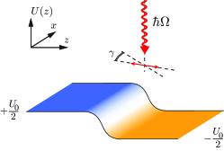
Figure 1: (Colour online) Graphene junction irradiated by an electromagnetic wave.

Result. We find the photocurrent as

$$I=\kappa\frac{e^{3}W}{\hbar cF}\left(\frac{U_{0}}{\hbar\Omega}\right)^{\frac{3}{2}}S\sin^{2}\gamma,$$ (1)

where $\gamma$ is the angle between polarization plane of the light and the potential barrier (axis $x$ in Fig. 1), $S$ is the radiation intensity, $W$ is the width of the strip, $F$ is the characteristic slope of the potential, and $\kappa$ is a constant of order unity.

Equation (1) indicates that the photocurrent vanishes if the polarization plane is parallel to the barrier ($\gamma=0$). In fact, it does not vanish completely, but acquires an extra power of the small parameter $U_{0}/\hbar\Omega\ll 1$,

$$I_{\|}=\kappa_{\|}\frac{e^{3}W}{\hbar cF}\left(\frac{U_{0}}{\hbar\Omega}\right)^{\frac{5}{2}}S,$$ (2)

$\kappa_{\|}$ is another constant of order unity.

Coefficients $\kappa$ and $\kappa_{\|}$ can be evaluated exactly for any particular form of the potential barrier. For instance, if the slope $F$ of the potential is constant on the interval from $z=-U_{0}/(2F)$ to $z=U_{0}/(2F)$ and zero otherwise, then $\kappa=8/3$ and $\kappa_{\|}=32/15$.

Model. The Hamiltonian of electrons in irradiated graphene in each valley reads

$$\hat{\cal H}=v\hat{\boldsymbol{\sigma}}\left[{\bf p}-{e}{c}^{-1}{\bf A}(t)\right]+U(z),$$ (3)

where the vector potential ${\bf A}(t)$ accounts for the external electromagnetic field (EF). For a linearly polarized wave one can choose

$${\bf A}(t)={c}{\Omega}^{-1}{\bf E}\cos(\Omega t).$$ (4)

The “pseudospin” ${\boldsymbol{\sigma}}$ in Eq. (3) is the spin-1/2 operator defined on the space of the two sublattices in graphene. The characteristic size of the step-like barrier lies typically within dozens of nanometers (see, e.g., Ref. Xia et al., 2009a), not exceeding the mean free path, so the transport in absence of radiation may be considered ballistically.

Scattering off photons. The dynamics of electrons affected by light has been considered microscopically in Ref. Syzranov et al., 2008. We provide here a simple semiqualitative picture describing the main features of this dynamics.

The light strongly affects electron motion only close to the “resonant points”, where the splitting $2vp$ between the conduction and valence bands matches the photon energy $\hbar\Omega$. Far from the resonant points the radiation weakly affects electron dynamics and can be neglected. The motion between the resonant points can be considered semiclassically. Electron velocity there has a constant value $v$, as follows from Eq. (3) at ${\bf A}=0$.

The rate of the radiation-induced transitions between the conduction and the valence bands,

$$\Gamma={2\pi}{\hbar}^{-1}\Delta^{2}\sin^{2}\beta\>\delta(2vp-\hbar\Omega),$$ (5)

may be viewed at small radiation intensities as a mere Fermi-golden-rule result. Here the “dynamical gap”Syzranov et al. (2008)

$$\Delta={v|e|E}/({2\Omega})$$ (6)

characterizes the strength of the radiation and $\beta$ is the angle between the electron momentum and the light polarization plane. The delta function guarantees that the transitions occur only at the resonant points. During the light-induced scattering, electron momentum ${\bf p}$ does not change, but the pseudospin flips and the energy increases (decreases) by $\hbar\Omega$ when absorbing (emitting) a photon.

Let $\alpha$ be the angle between the classical electron momentum ${\bf p}$ and the potential gradient $dU/d{\bf r}$. Integrating Eq. (5) over time and using that $\dot{{\bf p}}=-dU/d{\bf r}$ we find the probability of electron scattering at the resonant point

$${\cal L}(\beta,\alpha)={\pi\Delta^{2}\sin^{2}\beta}/({vF\cos\alpha}).$$ (7)

If an electron runs against a resonant point when moving along a certain classical trajectory, it scatters with probability ${\cal L}$ or continues its motion undisturbed by the radiation along the same trajectory with probability $1-{\cal L}$.

The above results, Eqs. (5) and (7), are obtained perturbatively in the limit of small $\Delta$ and thus require sufficiently small radiation powers. One can also derive Eqs. (5) and (7) explicitly by solving the Schrödinger equation for electrons in presence of EF or using the kinetic equationSyzranov et al. (2008). The condition of smallness of the radiation power reads ${\cal L}\ll 1$ and corresponds to the most experimentally relevant range of the system parameters.

Formula for the current. The previous generic picture of the light-affected electron dynamics in a nonuniform potential allows one to find the electron trajectories and to calculate the photocurrent asSyzranov et al. (2008)

$$I=4W\sum_{n}\int\frac{d{\bf p}}{(2\pi\hbar)^{2}}{\bf v}_{\|}P_{n}({\bf p})\left\{f[\varepsilon({\bf p})]-f[\varepsilon({\bf p})+n\hbar\Omega]\right\},$$ (8)

where the integration is carried out over the incoming electron momenta ${\bf p}$ in the left lead, ${\bf v}_{\|}$ is the respective longitudinal velocity, $P_{n}({\bf p})$ the probability for an electron outgoing from the left lead to penetrate into the right lead absorbing $n$ photons, $f(\varepsilon)$ is the equilibrium distribution function in both leads, and $W$ the width of the graphene strip. Equation (8) is, in fact, the Landauer formula generalized to account for the inelastic processes of photon absorption/emission.

In principle, our scheme of calculations follows that of Ref. Syzranov et al., 2008: We have to count all the classical trajectories corresponding to the inelastic electron transmission from the left to the right lead and then, using Eq. (8), calculate the value of the photocurrent. In the case of a shallow potential barrier, $U_{0}\ll\hbar\Omega$, studied in the present Brief Report, we are dealt with a greater variety of electron paths than in the previously studied case of a relatively high potentialSyzranov et al. (2008). Let us consider these trajectories in detail.

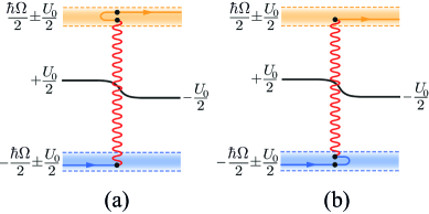
Figure 2: (Colour online) Inelastic penetration of an electron from the left to the right lead. The reflection from the potential barrier must occur either before (a) or after (b) the photon absorption.

Electron trajectories. As is follows from the resonance condition $\hbar\Omega=2vp$, the kinetic energies of an electron before (after) and after (before) the photon absorption (emission) equal, respectively, $vp=\hbar\Omega/2$ and $vp=-\hbar\Omega/2$. Hence photons can be absorbed only by incident electrons in the narrow energy band (Fig. 2)

$$-{\hbar\Omega}/{2}-{U_{0}}/{2}<\varepsilon<-{\hbar\Omega}/{2}+{U_{0}}/{2},$$ (9)

far below the Fermi level. So long as the latter has the same order of magnitude as $U_{0}$, its exact position is not important for the photocurrent.

Each electron with energy in the interval (9) and with a sufficiently small transverse momentum

$$vp_{\bot}<{\hbar\Omega}/{2},$$ (10)

inevitably meets a resonant point on its way from one lead to the other. Assume an electron incident from the left lead absorbs a photon at the very first resonant point I, Fig. 3(a). Before and after the absorption, its longitudinal velocity is directed, respectively, to and from the right lead. The velocity reversal may result in the return to the left lead, as shown by the orange (gray) line in Fig. 3(a). The electron, however, may also penetrate into the right lead and thus contribute to the photocurrent if it is reflected from the potential barrier after the photon absorption [see the orange (gray) solid line in Fig. 3(a)]. As the transverse momentum $p_{\bot}$ is conserved during the motion, $\varepsilon+\hbar\Omega$ and $U_{0}/2$ are, respectively, the full energy and the potential in the left lead, the return to this lead does not occur if and only if

$$\varepsilon+\hbar\Omega-vp_{\bot}<{U_{0}}/{2}.$$ (11)

Thus, we have shown that the charge carriers, which absorb photons at their first resonant points and satisfy conditions (9)-(11), contribute to the photocurrent.

What if the photon absorption at the first resonant point did not happen? Then the electron can proceed further to the other lead, meeting no other resonant points, or it can turn back, Fig. 3, provided

$$-\varepsilon-U_{0}<vp_{\bot}.$$ (12)

In the latter case the second resonant point II will be reached, for the longitudinal momentum decreases monotonously up to a certain turning point and then grows again. The sign of the longitudinal velocity at the second resonant point is opposite to that at the first one, so after the reflection the electron moves towards the right lead, along the orange (gray) line in Fig. 3(b). Then, since the momentum of the electron grows monotonously, neither resonant nor turning points can be met further.

Therefore, each electron, whose energy and momenta satisfy conditions (9), (10), and (12) can contribute to the photocurrent upon the photon absorption at point II.

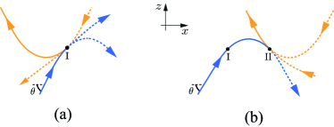
Figure 3: (Colour online) Classical trajectories of electrons incident on the potential barrier. Photon absorption occurs at (a) the first resonant point (b) the second resonant point. Solid lines show the paths that contribute to the photocurrent, dashed lines show the other possible trajectories. Blue (black) and orange (gray) lines correspond, respectively, to the motion in the valence and the conduction bands.

Clearly, elastic penetration from one lead to another is also possible, but, according to Eq. (8), does not contribute to the photocurrent. We have considered then all the scenarios of the light-assisted transmission from left to right, the contribution with $n=+1$ in Eq. (8). In principle, we are also to deal with electrons that absorb a photon on their way from right to left. It is more convenient, however, to consider the time-reversed processes and speculate in terms of the states outgoing from the same left lead and emitting a photon at the resonant points. Indeed, in Eq. (8) these processes are accounted for by the terms with $n=-1$, whereas the integration is carried out over the states in the left lead only.

The energies of the charge carriers, that can emit photons, lie in the range

$${\hbar\Omega}/{2}-{U_{0}}/{2}<\varepsilon<{\hbar\Omega}/{2}+{U_{0}}/{2}.$$ (13)

The reflection from the potential barrier without emitting a photon is not possible, for the longitudinal momentum of the electrons in the conduction band grows monotonously as the potential decreases. This forbids the processes analogous to what is shown in Fig. 3(b). Similarly, if an emission occurs at a resonant point, electron inevitably returns to the left lead.

Thus, there is no contribution to the photocurrent from the energy interval (13), and one has to take into account only the processes shown by solid lines in Fig. 3. Each of this processes involves at least one piece of a classical trajectory reflecting from the potential barrier. In the shallow potential under consideration the reflection is possible only during the motion nearly parallel to the barrier (axis $x$). Hence, the photocurrent found in the present Brief Report should be significantly smaller than that studied before in Ref. Syzranov et al., 2008 at large ratio $U_{0}/\hbar\Omega$. In the latter case nearly all electrons rebound from the barrier and photon absorption assists hopping from one trajectory of reflecting type to another such trajectory, similarl to what is shown in Fig. 3 by the solid lines. As we have shown, at $U_{0}/\hbar\Omega\ll 1$ the structure of electron paths is more diverse and very few of them contribute to the photocurrent.

Integration over the electron states. We must take into account the contributions to the photocurrent of electrons with momenta $p$ in the left lead, such that

$${\hbar\Omega}/({2v})<p<{\hbar\Omega}/({2v})+{U_{0}}/{v},$$ (14)

[cf., Eq. (9)] and incident at angles $\theta$ between the momenta ${\bf p}$ and the barrier that lie in one of the two intervals

$$\sqrt{2}\left[1-{\hbar\Omega}/({2vp})\right]^{{1}/{2}}<\theta<2\left[1-{\hbar\Omega}/({2vp})\right]^{{1}/{2}},$$ (15)

$$\sqrt{2}\left[1-{\hbar\Omega}/({2vp})\right]^{{1}/{2}}<\theta<\left[{2U_{0}}/({vp})\right]^{{1}/{2}},$$ (16)

corresponding, respectively, to Figs. 3(a) and 3(b).

The photon absorption at low radiation powers occurs with small probability

$${\cal L}={\pi\Delta^{2}\sin^{2}\gamma}/{\theta_{\mathrm{res}}},$$ (17)

where $\theta_{\mathrm{res}}$ is the angle between the momentum and the barrier at the resonant point, determined by the transverse momentum conservation law

$$p\cos\theta={\hbar\Omega}\cos\theta_{\mathrm{res}}\>/({2v}).$$ (18)

In Eqs. (15)-(17) we used the smallness of angle $\theta$.

Performing in Eq. (8) the integration over the intervals (14)-(16) of momenta and angles and substituting the probability $P_{+1}({\bf p})$ by ${\cal L}$, Eq. (17), we arrive at the main results of our Brief Report, Eqs. (1) and (2).

Physical interpretation. Equation (1) indicates that the photocurrent quickly decreases with wavelength in the range of photon energies exceeding the height of the potential barrier. Indeed, only electrons with energies close to $\pm\hbar\Omega/2$ participate in the photon-assisted transport. With increasing this energy the shallow potential becomes more transparent and has a lesser effect on electron motion, leading to the decrease of the photocurrent.

Since the energies of the involved electrons lie far below or far above the Fermi level, the photocurrent weakly depends on the background gate voltage. The dependency on the polarization direction $\propto\sin^{2}\gamma$ can be understood as follows. The photocurrent comes mainly from electrons moving nearly parallel to the barrier, as the others’ motion is unimpeded by the potential. The light absorption rate is proportional to the square of the component of the electric field $E_{\bot}$ perpendicular to the electron velocity, where $E_{\bot}\propto\sin\gamma$ for the specified electrons.

Albeit the photon absorption occurs far from the Dirac point and thus its description applies as well to an ordinary semiconductor, the dependency of the photocurrent on the radiation frequency $\Omega$, Eqs. (1) and (2), is determined by the bandstructure of graphene. Because there is no gap between the conduction and the valence bands, the photocurrent in graphene does not vanish even at very low frequencies, contrary to the case of an ordinary semiconductor.

The dependency of the current on the polarization can be used to separate the resonant photon absorption, considered here, from the other possible mechanisms of generating the photocurrent (e.g., a nonuniform heating of the sample by light). In the latter case phonons may play the same role as photons, but there would be no polarization dependency of the current.

Estimation. Let us estimate the value of the photocurrent for the typical device parametersXia et al. (2009a). For $\hbar\Omega=2e\mathrm{V}$, $U_{0}=50\mathrm{m}e\mathrm{V}$, $W=0.6\mu\mathrm{m}$, $S=13\mathrm{kW}/\mathrm{cm}^{2}$, and the characteristic size of the potential step $L=100\mathrm{nm}$ ($F=U_{0}/L$) we obtain from Eq. (1) at $\gamma=\pi/2$ the current $I\approx 12\mathrm{nA}$, in agreement with the characteristic values of the current measured in Ref. Xia et al., 2009a. In principle, the recombination length of photoexcited charge carriers may be comparable with $L$, then one should anticipate an attenuation of the current within an order of magnitude. As we mentioned before, checking its dependency on polarization could verify and help one to further investigate the mechanism of the current generation.

Conclusion. We calculated photocurrent in a graphene junction irradiated by light with the photon energy $\hbar\Omega$ considerably exceeding the characteristic height $U_{0}$ of the potential. The result is significantly smaller than the photocurrent in the case $\hbar\Omega\lesssim U_{0}$. It strongly depends on the polarization of light and is weakly affected by the background gate voltage. We thank M.V. Fistul for discussions. Our work has been supported financially by SFB Transregio 12 and SFB 491.

References

- Bonaccorso et al. (2010) F. Bonaccorso, Z. Sun, T. Hasan, and A. C. Ferrari, Nature Photonics 4, 611 (2010).
- Fistul et al. (2010) M. V. Fistul, S. V. Syzranov, A. M. Kadigrobov, and K. B. Efetov, Phys. Rev. B 82, 121409(R) (2010).
- Oka and Aoki (2009) T. Oka and H. Aoki, Phys. Rev. B 79, 081406(R) (2009); J. Karch, P. Olbrich, M. Schmalzbauer et al., Phys. Rev. Lett. 105, 227402 (2010a).
- Xia et al. (2009a) F. Xia, T. Mueller, R. Golizadeh-Mojarad et al., Nano Lett. 9, 1039 (2009a).
- Xia et al. (2009b) F. Xia, T. Mueller, Y. Ming Lin et al., Nano Lett. 4, 839 (2009b); T. Mueller, F. Xia, M. Freitag, J. Tsang, and P. Avouris, Phys. Rev. B 79, 245430 (2009); T. Mueller, F. Xia, and P. Avouris, Nature Photon. 4, 297 (2010).
- Park et al. (2009) J. Park, Y. H. Ahn, and C. Ruiz-Vargas, Nano Lett. 9, 1742 (2009).
- Xu et al. (2010) X. Xu, N. M. Gabor, J. S. Alden et al., Nano Lett. 10, 562 (2010).
- Syzranov et al. (2008) S. V. Syzranov, M. V. Fistul, and K. B. Efetov, Phys. Rev. B 78, 045407 (2008).
- Karch et al. (2010b) J. Karch, P. Olbrich, M. Schmalzbauer et al., e-print arXiv: eprint 1002.1047v1.
- Entin et al. (2010) M. V. Entin, L. I. Magarill, and D.L.Shepelyansky, Phys. Rev. B 81, 165441 (2010).