Long runs under point conditioning. The real case.

Abstract

This paper presents a sharp approximation of the density of long runs of a random walk conditioned on its end value or by an average of a functions of its summands as their number tends to infinity. The conditioning event is of moderate or large deviation type. The result extends the Gibbs conditional principle in the sense that it provides a description of the distribution of the random walk on long subsequences. An algorithm for the simulation of such long runs is presented, together with an algorithm determining their maximal length for which the approximation is valid up to a prescribed accuracy.

1 Introduction and notation

1.1 Context and scope

This paper explores the asymptotic distribution of a random walk conditioned on its final value as the number of summands increases. Denote $\mathbf{X}_{1}^{n}:=\left(\mathbf{X}_{1}\mathbf{,..,X}_{n}\right)$  a set of $n$ independent copies of a real random variable $\mathbf{X}$ with density $p$ on $\mathbb{R}$ and $\mathbf{S}_{1}^{n}:=\mathbf{X}_{1}+.$..$+\mathbf{X}_{n}.$  We consider approximations of the density of the vector $\mathbf{X}_{1}^{k}\mathbf{=}\left(\mathbf{X}_{1}\mathbf{,..,X}_{k}\right)$ on $\mathbb{R}^{k}$ when $\mathbf{S}_{1}^{n}=n\left(a_{n}\sqrt{Var\mathbf{X}}+E\mathbf{X}\right)$ and $a_{n}$ is either fixed different from $0$ or tends slowly to $0$ and $k:=k_{n}$ is an integer sequence such that

$$0\leq\lim\sup_{n\rightarrow\infty}k/n\leq 1$$ (1)

together with

$$\lim_{n\rightarrow\infty}n-k=\infty.$$ (2)

Therefore we may consider the asymptopic behavior of the density of the trajectory of the random walk on long runs. For sake of applications we also address the case when $\mathbf{S}_{1}^{n}$ is substituted by $\mathbf{U}_{1}^{n}:=f\left(\mathbf{X}_{1}\right)+...+f\left(\mathbf{X}_{n}\right)$ for some real valued measurable function $f$, and when the conditioning event writes $\left(\mathbf{U}_{1}^{n}=n\left(a_{n}\sqrt{Varf\left(\mathbf{X}\right)}+Ef\left(\mathbf{X}\right)\right)\right).$

The interest in this question stems from various sources. When $k$ is fixed (typically $k=1$) this is a version of the Gibbs Conditional Principle which has been studied extensively for fixed $a_{n}$, therefore under a large deviation condition. Diaconis and Freedman [8] have considered this issue also in the case $k/n\rightarrow\theta$ for $0\leq\theta<1$, in connection with de Finetti’s Theorem for exchangeable finite sequences. Their interest was related to the approximation of the density of $\mathbf{X}_{1}^{k}$ by the product density of the summands $\mathbf{X}_{i}$’s, therefore on the permanence of the independence of the $\mathbf{X}_{i}$’s under conditioning. Their result is in the spirit of van Camperhout and Cover [15] and to be paralleled with Csiszar’s [4] asymptotic conditional independence result, when the conditioning event is $\left(\mathbf{S}_{1}^{n}>n\left(a_{n}\sqrt{Var\mathbf{X}}+E\mathbf{X}\right)\right)$ with $a_{n}$ fixed and positive. In the same vein and under the same large deviation condition Dembo and Zeitouni [5] considered similar problems. This question is also of importance in Statistical Physics. Numerous papers pertaining to structural properties of polymers deal with this issue, and we refer to [6] and [7] for a description of those problems and related results. In the moderate deviation case Ermakov [10] also considered a similar problem when $k=1.$ Although out of the scope of the present paper the result which is presented here is a cornerstone in the development of fast Importance Sampling procedures for rare event simulation; see a first attempt in this direction in [3]. In Statistics, $M-$ estimators have the same weak behavior as the empirical mean of their influence functions on the sampling points in the moderate deviation zone. Simulating samples under a given value of the $M-$estimator leads to improved test procedures under small $p-$values.

We exhibit the change in the dependence structure of the $\mathbf{X}_{i}$’s under the conditioning as $k/n\rightarrow 1$ and provide an explicit and constructive solution to the approximation scheme. The approximating density is obtained as an adaptive change in the classical tilting argument combined with an adaptive change in the variance. Also when $k=o(n)$ our result improves on existing ones since it provides a sharp approximation of the conditional density. The present result is optimal in the sense that it coincides with the exact conditional density in the gaussian case.

The crucial aspect of our result is the following. The approximation of the density of $\mathbf{X}_{1}^{k}$ is not performed on the sequence of entire spaces $\mathbb{R}^{k}$ but merely on a sequence of subsets of $\mathbb{R}^{k}$ which bear the trajectories of the conditioned random walk with probability going to $1$ as $n$ tends to infinity; therefore the approximation is performed on typical paths. The reason which led us to consider approximation in this peculiar sense is twofold. First the approximation on typical paths is what is in fact needed for the applications of the present results in the field of simulation and of rare event analysis; second it avoids a number of technical conditions which are necessary in order to get an approximation on all $\mathbb{R}^{k}$ and which are indeed central in the above mentioned works; those conditions pertain to the regularity of the characteristic function of the underlying density $p$ in order to get a good approximation in remote regions of $\mathbb{R}^{k}$. Since the approximation is handled on paths generated under the conditional density of the $\mathbf{X}_{i}$’s under the conditioning, much is known on the region of $\mathbb{R}^{k}$ which is reached with large probability by the conditioned random walk, through the analysis of the large values of the $\mathbf{X}_{i}$’s.

For sake of numerical applications we provide explicit algorithms for the generation of such random walks together with a number of comments for the practical implementation. Also an explicit rule for the maximal value of $k$ compatible with a given accuracy of the approximating scheme is presented and numerical simulation supports this rule; an algorithm for its calculation is presented.

1.2 Notation and hypotheses

In the context of the point conditioning

$$\mathcal{E}_{n}:=\left(\mathbf{S}_{1}^{n}=n\left(a_{n}\sqrt{Var\mathbf{X}}+E\mathbf{X}\right)\right)$$

the hypotheses are as below. The case when $\mathbf{S}_{1}^{n}$ is substituted by $\mathbf{U}_{1}^{n}$ is postponed to Section 3, together with the relevant hypotheses and notation.

We assume that $\mathbf{X}$ satisfies the Cramer condition, i.e. $\mathbf{X}$ has a finite moment generating function $\Phi(t):=E\exp t\mathbf{X}$ in a non void neighborhood of $0;$ denote

$$m(t):=\frac{d}{dt}\log\Phi(t)$$

and

$$s^{2}(t):=\frac{d}{dt}m(t).$$

The values of $m(t)$ and $s^{2}$ are the expectation and the variance of the tilted density

$$\pi^{\alpha}(x):=\frac{\exp tx}{\Phi(t)}p(x)$$ (3)

where $t$ is the only solution of the equation $m(t)=\alpha$ when $\alpha$ belongs to the support of $\mathbf{X}$, see Barnfoff-Nielsen [2] for details. Denote $\Pi^{\alpha}$ the probability measure with density $\pi^{\alpha}$.

We also assume that the characteristic function of $\mathbf{X}$ is in $L^{r}$ for some $r\geq 1$ which is necessary for the Edgeworth expansions to be performed.

The probability measure of the random vector $\mathbf{X}_{1}^{n}$ on $\mathbb{R}^{n}$ conditioned upon $\mathcal{E}_{n}$ is denoted $\mathfrak{P}_{n}.$ We also denote $\mathfrak{P}_{n}$ the corresponding distribution of $\mathbf{X}_{1}^{k}$ conditioned upon $\mathcal{E}_{n}$; the vector $\mathbf{X}_{1}^{k}$ then has a density with respect to the Lebesgue measure on $\mathbb{R}^{k}$ for $1\leq k<n$ ,which will be denoted $\mathfrak{p}_{n}$, which might seem ambiguous but recalls that the conditioned distribution pertains to the value of $\mathbf{S}_{1}^{n},$ from which the density of $\mathbf{X}_{1}^{k}$ is obtained. For a generic r.v. $\mathbf{Z}$ with density $p$, we denote $p\left(\mathbf{Z}=z\right)$ the value of $p$ at point $z.$

This paper is organized as follows. Section 2 presents the approximation scheme for the conditional density of $\mathbf{X}_{1}^{k}$ under the point conditioning sequence $\mathcal{E}_{n}.$ In section 3, it is extended to the case when the conditioning family of events writes $\left(\mathbf{U}_{1}^{n}=n\left(a_{n}\sqrt{Varf\left(\mathbf{X}\right)}+Ef\left(\mathbf{X}\right)\right)\right).$ The value of $k$ for which this approximation is fair is discussed; an algorithm for the implementation of this rule is proposed. Section 4 presents an algorithm for the simulation of random variables under the approximating scheme. We have kept the main steps of the proofs in the core of the paper; some of the technicalities is left to the Appendix.

2 Random walks conditioned on their sum

We introduce a positive sequence $\epsilon_{n}$ which satisfies

$$\lim_{n\rightarrow\infty}\epsilon_{n}\sqrt{n-k} =\infty$$ (E1)

$$\lim_{n\rightarrow\infty}\epsilon_{n}\left(\log n\right)^{2} =0.\text{ }$$ (E2)

It will be shown that $\epsilon_{n}\left(\log n\right)^{2}$ is the rate of accuracy of the approximating scheme.

We denote $a$ the generic term of the bounded sequence $\left(a_{n}\right)_{n\geq 1},$ which we assume positive, without loss of generality . The event $\mathcal{E}_{n}$ is of moderate or large deviation type, since we assume that

$$\lim_{n\rightarrow\infty}\frac{a^{2}}{\epsilon_{n}\left(\log n\right)^{2}}=\infty.$$ (A)

The case when $a$ does not depend on $n$ satisfies (A) for any sequence $\epsilon_{n}$ under (E1,2). Conditions (A) and (E1,2) jointly imply that $a$ cannot satisfy $\sqrt{n}a\rightarrow c$ for some fixed $c;$ the Central Limit zone is not covered by our result. In order that there exists a sequence $\epsilon_{n}$ such that the approximation of $\mathfrak{p}_{n}$ holds with rate $\epsilon_{n}\left(\log n\right)^{2}\rightarrow 0$, a sufficient condition on $a_{n}$ is

$$\lim_{n\rightarrow\infty}\frac{\sqrt{n}a^{2}}{(\log n)^{2}}=\infty$$ (4)

which covers both the moderate and the large deviation cases.

Under these assumptions $k$ can be fixed or can grow together with $n$ with the restriction that $n-k$ should tend to infinity; when $a$ is fixed this rate is governed through (E1) (or reciprocally given $k$ ,$\epsilon_{n}$ is governed by $k$) independently on $a.$ In the moderate deviation case for a given sequence $a$ close to $0$, $\epsilon_{n}$ has rapid decrease, which in turn forces $n-k$ to grow rapidly.

In this section we assume that $\mathbf{X}$ has expectation $0$ and variance $1.$ For clearness the dependence in $n$ of all quantities involved in the coming development is omitted in the notation.

2.1 Approximation of the density of the runs

Let $a=a_{n}$ denote the current term of a sequence satisfying (A). Define a density $g_{a}(y_{1}^{k})$ on $\mathbb{R}^{k}$ as follows. Set

$$g_{0}(\left.y_{1}\right|y_{0}):=\pi^{a}(y_{1})$$

with $y_{0}$ arbitrary, and for $1\leq i\leq k-1$ define $g_{i}(\left.y_{i+1}\right|y_{1}^{i})$ recursively.

Set $t_{i}$ the unique solution of the equation

$$m_{i}:=m(t_{i})=\frac{n}{n-i}\left(a-\frac{s_{1}^{i}}{n}\right)$$ (5)

where $s_{1}^{i}:=y_{1}+...+y_{i}.$ The tilted adaptive family of densities $\pi^{m_{i}}$ is the basic ingredient of the derivation of approximating scheme. Let

$$s_{i}^{2}:=\frac{d^{2}}{dt^{2}}\left(\log E_{\pi^{m_{i}}}\exp t\mathbf{X}\right)\left(0\right)$$

and

$$\mu_{j}^{i}:=\frac{d^{j}}{dt^{j}}\left(\log E_{\pi^{m_{i}}}\exp t\mathbf{X}\right)\left(0\right),\text{ }j=3,4$$

which are the second , third and fourth centered moments of $\pi^{m_{i}}.$ Let

$$g_{i}(\left.y_{i+1}\right|y_{1}^{i})=C_{i}p(y_{i+1})\mathfrak{n}\left(a+\alpha\beta,\alpha,y_{i+1}\right)$$ (6)

where $\mathfrak{n}\left(\mu,\tau,x\right)$ is the normal density with mean $\mu$ and variance $\tau$ at $x$. Here

$$\alpha=s_{i}^{2}\left(n-i-1\right)$$ (7)

$$\beta=t_{i}+\frac{\mu_{3}^{i}}{2s_{i}^{2}\left(n-i-1\right)}$$ (8)

and $C_{i}$ is a normalizing constant.

Define

$$g_{a}(y_{1}^{k}):=\prod_{i=0}^{k-1}g_{i}(\left.y_{i+1}\right|y_{1}^{i}).$$ (9)

We then have

Theorem 1

Assume that (E1,2) holds together with (A). Let $Y_{1}^{n}$ be a sample with distribution $\mathfrak{P}_{n}.$ Then

$$\mathfrak{p}_{n}\left(Y_{1}^{k}\right):=p(\left.\mathbf{X}_{1}^{k}=Y_{1}^{k}\right|\mathbf{S}_{1}^{n}=na)=g_{a}(Y_{1}^{k})(1+o_{\mathfrak{P}_{n}}(\epsilon_{n}\left(\log n\right)^{2})).$$ (10)

Proof. The proof uses Bayes formula to write $p(\left.\mathbf{X}_{1}^{k}=Y_{1}^{k}\right|\mathbf{S}_{1}^{n}=na)$ as a product of $k$ conditional densities of individual terms of the trajectory evaluated at $Y_{1}^{k}$. Each term of this product is approximated through an Edgeworth expansion which together with the properties of $Y_{1}^{k}$ under $\mathfrak{P}_{n}$ concludes the proof. This proof is rather long and we have differed its technical steps to the Appendix.

Denote $\Sigma_{1}^{0}=0$, $\Sigma_{1}^{1}:=Y_{1}$    and $\Sigma_{1}^{i}:=\Sigma_{1}^{i-1}+Y_{i}.$ It holds

$$p(\left.\mathbf{X}_{1}^{k}=Y_{1}^{k}\right|\mathbf{S}_{1}^{n} =na)=p(\left.\mathbf{X}_{1}=Y_{1}\right|\mathbf{S}_{1}^{n}=na)$$ (11)

$$\prod_{i=1}^{k-1}p(\left.\mathbf{X}_{i+1}=Y_{i+1}\right|\mathbf{X}_{1}^{i} =Y_{1}^{i},\mathbf{S}_{1}^{n}=na)$$

$$=\prod_{i=0}^{k-1}p\left(\left.\mathbf{X}_{i+1}=Y_{i+1}\right|\mathbf{S}_{i+1}^{n}=na-\Sigma_{1}^{i}\right)$$

using independence of the r.v’s $\mathbf{X}_{i}^{\prime}s$.

We make use of the following property which states the invariance of conditional densities under the tilting: For $1\leq i\leq j\leq n,$ for all $a$ in the range of $\mathbf{X},$ for all $u$ and $s$

$$p\left(\left.\mathbf{S}_{i}^{j}=u\right|\mathbf{S}_{1}^{n}=s\right)=\pi^{a}\left(\left.\mathbf{S}_{i}^{j}=u\right|\mathbf{S}_{1}^{n}=s\right).$$ (12)

Define $t_{i}$ through

$$m(t_{i})=\frac{n}{n-i}\left(a-\frac{\Sigma_{1}^{i}}{n}\right)$$

a function of the past r.v’s $Y_{1}^{i}$ and set $m_{i}:=m(t_{i})$ and $s_{i}^{2}:=s^{2}(t_{i}).$ By (12)

$$p\left(\left.\mathbf{X}_{i+1}=Y_{i+1}\right|\mathbf{S}_{i+1}^{n}=na-\Sigma_{1}^{i}\right)$$

$$=\pi^{m_{i}}\left(\left.\mathbf{X}_{i+1}=Y_{i+1}\right|\mathbf{S}_{i+1}^{n}=na-\Sigma_{1}^{i}\right)$$

$$=\pi^{m_{i}}\left(\mathbf{X}_{i+1}=Y_{i+1}\right)\frac{\pi^{m_{i}}\left(\mathbf{S}_{i+2}^{n}=na-\Sigma_{1}^{i+1}\right)}{\pi^{m_{i}}\left(\mathbf{S}_{i+1}^{n}=na-\Sigma_{1}^{i}\right)}$$

where we used the independence of the $\mathbf{X}_{j}$’s under $\pi^{m_{i}}.$ A precise evaluation of the dominating terms in this lattest expression is needed in order to handle the product (11).

Under the sequence of densities $\pi^{m_{i}}$ the i.i.d. r.v’s $\mathbf{X}_{i+1},...,\mathbf{X}_{n}$ define a triangular array which satisfies a local central limit theorem, and an Edgeworth expansion. Under $\pi^{m_{i}}$, $\mathbf{X}_{i+1}$ has expectation $m_{i}$ and variance $s_{i}^{2}.$ Center and normalize both the numerator and denominator in the fraction which appears in the last display. Denote $\overline{\pi_{n-i-1}}$ the density of the normalized sum $\left(\mathbf{S}_{i+2}^{n}-(n-i-1)m_{i}\right)/\left(s_{i}\sqrt{n-i-1}\right)$ when the summands are i.i.d. with common density $\pi^{m_{i}}.$ Accordingly $\overline{\pi_{n-i}}$ is the density of $\left(\mathbf{S}_{i+1}^{n}-(n-i)m_{i}\right)/\left(s_{i}\sqrt{n-i}\right)$ under i.i.d. $\pi^{m_{i}}$ sampling. Hence, evaluating both $\overline{\pi_{n-i-1}}$ and its normal approximation at point $Y_{i+1},$

$$p\left(\left.\mathbf{X}_{i+1}=Y_{i+1}\right|\mathbf{S}_{i+1}^{n}=na-\Sigma_{1}^{i}\right)$$ (13)

$$=\frac{\sqrt{n-i}}{\sqrt{n-i-1}}\pi^{m_{i}}\left(\mathbf{X}_{i+1}=Y_{i+1}\right)\frac{\overline{\pi_{n-i-1}}\left(\left(m_{i}-Y_{i+1}\right)/s_{i}\sqrt{n-i-1}\right)}{\overline{\pi_{n-i}}(0)}$$

$$:=\frac{\sqrt{n-i}}{\sqrt{n-i-1}}\pi^{m_{i}}\left(\mathbf{X}_{i+1}=Y_{i+1}\right)\frac{N_{i}}{D_{i}}.$$

The sequence of densities $\overline{\pi_{n-i-1}}$ converges pointwise to the standard normal density under (E1) which implies that $n-k$ tends to infinity, and an Edgeworth expansion to the order 5 is performed for the numerator and the denominator. The main arguments used in order to obtain the order of magnitude of the envolved quantities are (i) a maximal inequality which controls the magnitude of $m_{i}$   for all $i$ between $0$ and $k-1$ (Lemma 13), (ii) the order of the maximum of the $Y_{i}^{\prime}s$ (Lemma 14). As proved in the Appendix, under (A)

$$N_{i}=\phi\left(-Y_{i+1}/\left(s_{i}\sqrt{n-i-1}\right)\right).A.B+O_{\mathfrak{P}_{n}}\left(\frac{1}{\left(n-i-1\right)^{3/2}}\right)$$ (14)

where $\phi$ is the standard normal density and,

$$A:=\left(1+\frac{aY_{i+1}}{s_{i}^{2}(n-i-1)}-\frac{a^{2}}{2s_{i}^{2}(n-i-1)}+\frac{o_{\mathfrak{P}_{n}}(\epsilon_{n}\log n)}{n-i-1}\right)$$ (15)

and

$$B:=\left(\begin{array}[]{c}1-\frac{\mu_{3}^{i}}{2s_{i}^{4}\left(n-i-1\right)}(a-Y_{i+1})\\ -\frac{\mu_{3}^{i}-s_{i}^{4}}{8s_{i}^{4}(n-i-1)}-\frac{15(\mu_{3}^{i})^{2}}{72s_{i}^{6}(n-i-1)}+\frac{O_{\mathfrak{P}_{n}}\left((\log n)^{2}\right)}{\left(n-i-1\right)^{2}}\end{array}\right)$$ (16)

The $O_{\mathfrak{P}_{n}}\left(\frac{1}{\left(n-i-1\right)^{3/2}}\right)$ term in (14) is uniform upon $\left(m_{i}-Y_{i+1}\right)/s_{i}\sqrt{n-i-1}.$ Turn back to (13) and do the same Edgeworth expansion in the demominator, which writes

$$D_{i}=\phi(0)\left(1-\frac{\mu_{3}^{i}-s_{i}^{4}}{8s_{i}^{4}(n-i)}-\frac{15(\mu_{3}^{i})^{2}}{72s_{i}^{6}(n-i)}\right)+O_{\mathfrak{P}_{n}}\left(\frac{1}{\left(n-i\right)^{3/2}}\right).$$ (17)

The terms in $g_{i}(\left.Y_{i+1}\right|Y_{1}^{i})$ follow from an expansion in the ratio of the two expressions (14) and (17) above. The gaussian contribution is explicit in (14) while the term $\exp\frac{\mu_{3}^{i}}{2s_{i}^{4}\left(n-i-1\right)}Y_{i+1}$ is the dominant term in $B$. Turning to (13) and comparing with (10) it appears that the normalizing factor $C_{i}$ in $g_{i}(\left.Y_{i+1}\right|Y_{1}^{i})$ compensates the term $\frac{\sqrt{n-i}}{\Phi(t_{i})\sqrt{n-i-1}}\exp\left(\frac{-a\mu_{3}^{i}}{2s_{i}^{2}(n-i-1)}\right),$ where the term $\Phi(t_{i})$ comes from $\pi^{m_{i}}\left(\mathbf{X}_{i+1}=Y_{i+1}\right).$ Further the product of the remaining terms in the above approximations in (14) and (17) turn to build the $1+o_{\mathfrak{P}_{n}}\left(\epsilon_{n}\left(\log n\right)^{2}\right)$ approximation rate, as claimed. Details are differed to the Appendix. This yields

$$p(\left.\mathbf{X}_{1}^{k}=Y_{1}^{k}\right|\mathbf{S}_{1}^{n}=na)=\left(1+o_{\mathfrak{P}_{n}}\left(\epsilon_{n}\left(\log n\right)^{2}\right)\right)\prod_{i=0}^{k-1}g_{i}(\left.Y_{i+1}\right|Y_{1}^{i})$$

which closes the proof of the Theorem.   

Remark 2

When the $\mathbf{X}_{i}$’s are i.i.d. with a standard normal density, then the result in the above approximation Theorem holds with $k=n-1$ stating that $p(\left.\mathbf{X}_{1}^{n-1}=x_{1}^{n-1}\right|\mathbf{S}_{1}^{n}=na)=g_{a}\left(x_{1}^{n-1}\right)$ for all $x_{1}^{n-1}$ in $\mathbb{R}^{n-1}$. This extends to the case when they have an infinitely divisible distribution. However formula (10) holds true without the error term only in the gaussian case. Similar exact formulas can be obtained for infinitely divisible distributions using (11) making no use of tilting. Such formula is used to produce Tables 1 and 2 in order to assess the validity of the selection rule for $k$ in the exponential case.

Remark 3

The density in (6) is a slight modification of $\pi^{m_{i}}.$ The modification from $\pi^{m_{i}}$ to $g_{i}$ is a small shift in the location parameter depending both on $a_{n}$ and on the skewness of $p$, and a change in the variance : large values of $\ \mathbf{X}_{i+1}$ have smaller weigth for large $i,$ so that the distribution of $\ \mathbf{X}_{i+1}$ tends to concentrate around $m_{i}$ as $i$ approaches $k.$

Remark 4

In the previous Theorem, as in Lemma 14, we use an Edgeworth expansion for the density of the normalized sum of the $n-$th row of some triangular array of row-wise independent r.v’s with common density. Consider the i.i.d. r.v’s $\mathbf{X}_{1},...,\mathbf{X}_{n}$ with common density $\pi^{a}(x)$ where $a$ may depend on $n$ but remains bounded. The Edgeworth expansion pertaining to the normalized density of $\mathbf{S}_{1}^{n}$ under $\pi^{a}$ can be derived following closely the proof given for example in [11], pp 532 and followings substituting the cumulants of $p$ by those of $\pi^{a}$. Denote $\varphi_{a}(z)$ the characteristic function of $\pi^{a}(x).$ Clearly for any $\delta>0$ there exists $q_{a,\delta}<1$ such that $\left|\varphi_{a}(z)\right|<$ $q_{a,\delta}$ and since $a$ is bounded, $\sup_{n}q_{a,\delta}<1.$ Therefore the inequality (2.5) in [11] p533 holds. With $\psi_{n}$ defined as in [11], (2.6) holds with $\varphi$ replaced by $\varphi_{a}$ and $a$ by $s(t_{a});$ (2.9) holds, which completes the proof of the Edgeworth expansion in the simple case. The proof goes in the same way for higher order expansions.

2.2 Sampling under the approximation

Applications of Theorem 1 in Importance Sampling procedures and in Statistics require a reverse result. So assume that $Y_{1}^{k}$ is a random vector generated under $G_{a}$ with density $g_{a}.$ Can we state that $g_{a}\left(Y_{1}^{k}\right)$ is a good approximation for $\mathfrak{p}_{n}\left(Y_{1}^{k}\right)$? This holds true. We state a simple Lemma in this direction.

Let $\mathfrak{R}_{n}$ and $\mathfrak{S}_{n}$ denote two p.m’s on $\mathbb{R}^{n}$ with respective densities $\mathfrak{r}_{n}$ and $\mathfrak{s}_{n}.$

Lemma 5

Suppose that for some sequence $\varepsilon_{n}$   which tends to $0$ as $n$ tends to infinity

$$\mathfrak{r}_{n}\left(Y_{1}^{n}\right)=\mathfrak{s}_{n}\left(Y_{1}^{n}\right)\left(1+o_{\mathfrak{R}_{n}}(\varepsilon_{n})\right)$$ (18)

as $n$ tends to $\infty.$ Then

$$\mathfrak{s}_{n}\left(Y_{1}^{n}\right)=\mathfrak{r}_{n}\left(Y_{1}^{n}\right)\left(1+o_{\mathfrak{S}_{n}}(\varepsilon_{n})\right).$$ (19)

Proof. Denote

$$A_{n,\varepsilon_{n}}:=\left\{y_{1}^{n}:(1-\varepsilon_{n})\mathfrak{s}_{n}\left(y_{1}^{n}\right)\leq\mathfrak{r}_{n}\left(y_{1}^{n}\right)\leq\mathfrak{s}_{n}\left(y_{1}^{n}\right)(1+\varepsilon_{n})\right\}.$$

It holds for all positive $\delta$

$$\lim_{n\rightarrow\infty}\mathfrak{R}_{n}\left(A_{n,\delta\varepsilon_{n}}\right)=1.$$

Write

$$\mathfrak{R}_{n}\left(A_{n,\delta\varepsilon_{n}}\right)=\int\mathbf{1}_{A_{n,\delta\varepsilon_{n}}}\left(y_{1}^{n}\right)\frac{\mathfrak{r}_{n}\left(y_{1}^{n}\right)}{\mathfrak{s}_{n}(y_{1}^{n})}\mathfrak{s}_{n}(y_{1}^{n})dy_{1}^{n}.$$

Since

$$\mathfrak{R}_{n}\left(A_{n,\delta\varepsilon_{n}}\right)\leq(1+\delta\varepsilon_{n})\mathfrak{S}_{n}\left(A_{n,\delta\varepsilon_{n}}\right)$$

it follows that

$$\lim_{n\rightarrow\infty}\mathfrak{S}_{n}\left(A_{n,\delta\varepsilon_{n}}\right)=1,$$

which proves the claim.   

As a direct by-product of Theorem 1 and Lemma 5 we obtain

Theorem 6

Assume (A), (E1,2). Then when $Y_{1}^{n}$ is generated under the distribution $G_{a}$ it holds

$$\mathfrak{p}_{n}\left(Y_{1}^{k}\right)=g_{a}(Y_{1}^{k})(1+o_{G_{a}}(\epsilon_{n}\left(\log n\right)^{2}))$$

with $\mathfrak{p}_{n}$ defined in (10).

3 Random walks conditioned by the mean of a function of their summands

This section extends the above results to the case when the conditioning event writes

$$\mathbf{U}_{1}^{n}:=f\left(\mathbf{X}_{1}\right)+...+f\left(\mathbf{X}_{n}\right)=n\left(\sigma a+\mu\right).$$ (20)

The function $f$ is real valued, $Ef\left(\mathbf{X}\right)=\mu$ and $Varf\left(\mathbf{X}\right)=\sigma^{2}.$ The characteristic function of the random variable $f\left(\mathbf{X}\right)$ is assumed to belong to $L^{r}$ for some $r\geq 1.$ As previously $a$ is assumed positive. Let $p_{\mathbf{X}}$ denote the density of the r.v. $\mathbf{X}$.

Assume

$$\phi_{f}(t):=E\exp tf\left(\mathbf{X}\right)<\infty$$

for $t$ in a non void neighborhood of $0.$ Define the functions $m_{f}(t),s_{f}^{2}(t)$ and $\mu_{f,3}(t)$ as the first, second and third derivatives of $\log\mathfrak{\phi}_{f}(t).$

Denote

$$\pi_{f}^{\alpha}(x):=\frac{\exp tf(x)}{\phi_{f}(t)}p_{\mathbf{X}}\left(x\right)$$

with $m_{f}(t)=\alpha$ and $\alpha$ belongs to the support of $P_{f}$, the distribution of $f\left(\mathbf{X}\right),$ with density $p_{f}.$ Conditions on $\phi_{f}(t)$ which ensure existence and uniqueness of $t$ are referred to as steepness properties, and are exposed in [2]

Assume that (A) holds and the sequence $\epsilon_{n}$ satisfies (E1,2).

3.1 Approximation of the density of the runs

Define a density $h_{\sigma a+\mu}(y_{1}^{k})$ with c.d.f. $H_{\sigma a+\mu}$ on $\mathbb{R}^{k}$ as follows. Set

$$h_{0}(\left.y_{1}\right|y_{0}):=\pi_{f}^{\sigma a+\mu}(y_{1})$$

with $y_{0}$ arbitrary and for $1\leq i\leq k-1$ define $h_{i}(\left.y_{i+1}\right|y_{1}^{i})$ recursively.

Set $t_{i}$ the unique solution of the equation

$$m_{i}:=m_{f}(t_{i})=\frac{n}{n-i}\left(\sigma a+\mu-\frac{u_{1}^{i}}{n}\right)$$ (21)

where $u_{1}^{i}:=f\left(y_{1}\right)+...+f\left(y_{i}\right).$

Define

$$h_{i}(\left.y_{i+1}\right|y_{1}^{i})=C_{i}p_{\mathbf{X}}(y_{i+1})\mathfrak{n}\left(\alpha\beta+\left(\sigma a+\mu\right),\alpha,f(y_{i+1})\right)$$ (22)

where $C_{i}$ is a normalizing constant. Here

$$\alpha=s_{f}^{2}(t_{i})\left(n-i-1\right)$$ (23)

$$\beta=t_{i}+\frac{\mu_{f,3}\left(t_{i}\right)}{2s_{f}^{4}(t_{i})\left(n-i-1\right)}.$$ (24)

Set

$$h_{\sigma a+\mu}\left(y_{1}^{k}\right):=\prod\limits_{i=0}^{k-1}h_{i}(\left.y_{i+1}\right|y_{1}^{i}).$$ (25)

Denote $\mathfrak{P}_{n}^{f}$ the distribution of $\mathbf{X}_{1}^{n}$ conditioned upon $\left(\mathbf{U}_{1}^{n}=n\left(\sigma a+\mu\right)\right)$ and $\mathfrak{p}_{n}^{f}$ its density when restricted on $\mathbb{R}^{k};$ therefore

$$\mathfrak{p}_{n}^{f}\left(\mathbf{X}_{1}^{k}=Y_{1}^{k}\right):=p(\left.\mathbf{X}_{1}^{k}=Y_{1}^{k}\right|\mathbf{U}_{1}^{n}=n\left(\sigma a+\mu\right)).$$ (26)

Theorem 7

Assume (A) and (E1,2) . Then (i)

$$\mathfrak{p}_{n}^{f}\left(\mathbf{X}_{1}^{k}=Y_{1}^{k}\right)=h_{\sigma a+\mu}(Y_{1}^{k})(1+o_{\mathfrak{P}_{n}^{f}}(\epsilon_{n}\left(\log n\right)^{2}))$$

and (ii)

$$\mathfrak{p}_{n}^{f}\left(\mathbf{X}_{1}^{k}=Y_{1}^{k}\right)=h_{\sigma a+\mu}(Y_{1}^{k})(1+o_{H_{\sigma a+\mu}}(\epsilon_{n}\left(\log n\right)^{2})).$$

Proof. We only sketch the initial step of the proof of (i), which rapidly follows the same track as that in Theorem 1. Denote $U_{i}^{j}:=f(Y_{i})+...+f(Y_{j}).$

As in the proof of  Theorem 1 evaluate

$$p\left(\left.\mathbf{X}_{i+1}=Y_{i+1}\right|\mathbf{U}_{i+1}^{n}=n\left(\sigma a+\mu\right)-U_{1}^{i}\right)$$

$$=p\left(\mathbf{X}_{i+1}=Y_{i+1}\right)\frac{p\left(\mathbf{U}_{i+2}^{n}=n\left(\sigma a+\mu\right)-U_{1}^{i+1}\right)}{p\left(\mathbf{U}_{i+1}^{n}=n\left(\sigma a+\mu\right)-U_{1}^{i}\right)}.$$

Use the tilting invariance under $\mathfrak{\pi}_{f}^{m_{i}}$ leading to

$$p\left(\left.\mathbf{X}_{i+1}=Y_{i+1}\right|\mathbf{U}_{i+1}^{n}=n\left(\sigma a+\mu\right)-U_{1}^{i}\right)$$

$$=\pi_{f}^{m_{i}}\left(\mathbf{X}_{i+1}=Y_{i+1}\right)\frac{\pi_{f}^{m_{i}}\left(\mathbf{U}_{i+2}^{n}=n\left(\sigma a+\mu\right)-U_{1}^{i+1}\right)}{\pi_{f}^{m_{i}}\left(\mathbf{T}_{i+1}^{n}=n\left(\sigma a+\mu\right)-U_{1}^{i}\right)}$$

$$=p\left(\mathbf{X}_{i+1}=Y_{i+1}\right)\frac{e^{t_{i}f\left(Y_{i+1}\right)}}{\phi_{f}(t_{i})}\frac{\pi_{f}^{m_{i}}\left(\mathbf{U}_{i+2}^{n}=n\left(\sigma a+\mu\right)-U_{1}^{i+1}\right)}{\pi_{f}^{m_{i}}\left(\mathbf{U}_{i+1}^{n}=n\left(\sigma a+\mu\right)-U_{1}^{i}\right)}$$

and proceed through the Edgeworth expansions in the above expression, following verbatim the proof of Theorem 1. We omit details. The proof of (ii) follows from Lemma 5   

3.2 How far is the approximation valid?

This section provides a rule leading to an effective choice of the crucial parameter $k$ in order to achieve a given accuracy bound for the relative error. The generic r.v. $\mathbf{X}$ has density $p_{\mathbf{X}}$ and $f\left(\mathbf{X}\right)$ has mean $\mu$ and variance $\sigma^{2}.$ The density $\mathfrak{p}_{n}^{f}$ is defined in (26). The accuracy of the approximation is measured through

$$ERE(k):=E_{h_{\sigma a+\mu}}1_{D_{k}}\left(Y_{1}^{k}\right)\frac{\mathfrak{p}_{n}^{f}\left(Y_{1}^{k}\right)-h_{\sigma a+\mu}\left(Y_{1}^{k}\right)}{\mathfrak{p}_{n}^{f}\left(Y_{1}^{k}\right)}$$

and

$$VRE(k):=Var_{h_{\sigma a+\mu}}1_{D_{k}}\left(Y_{1}^{k}\right)\frac{\mathfrak{p}_{n}^{f}\left(Y_{1}^{k}\right)-h_{\sigma a+\mu}\left(Y_{1}^{k}\right)}{\mathfrak{p}_{n}^{f}\left(Y_{1}^{k}\right)}$$ (27)

respectively the expectation and the variance of the relative error of the approximating scheme when evaluated on $D_{k}$ , the subset of $\mathbb{R}^{k}$  where $\left|h_{\sigma a+\mu}(Y_{1}^{k})/\mathfrak{p}_{n}^{f}\left(Y_{1}^{k}\right)-1\right|<\delta_{n}$ with $\epsilon_{n}\left(\log n\right)^{2}/\delta_{n}\rightarrow 0$ and $\delta_{n}\rightarrow 0;$ therefore $H_{\sigma a+\mu}\left(D_{k}\right)\rightarrow 1.$The r.v^′s $Y_{1}^{k}$ are sampled under $h_{\sigma a+\mu}.$ Note that the density $\mathfrak{p}_{n}^{f}$ is usually unknown. The argument is somehow heuristic and unformal; nevertheless the rule is simple to implement and provides good results. We assume that the set $D_{k}$   can be substituted by $\mathbb{R}^{k}$ in the above formulas, therefore assuming that the relative error has bounded variance, which would require quite a lot of work to be proved under appropriate conditions, but which seems to hold, at least in all cases considered by the authors. We keep the above notation omitting therefore any reference to $D_{k}$ .

Consider a two-sigma confidence bound for the relative accuracy for a given $k$, defining

$$CI(k):=\left[ERE(k)-2\sqrt{VRE(k)},ERE(k)+2\sqrt{VRE(k)}\right].$$

Let $\delta$ denote an acceptance level for the relative accuracy. Accept $k$ until $\delta$ belongs to $CI(k).$ For such $k$ the relative accuracy is certified up to the level $5\%$ roughly.

The calculation of $VRE(k)$ and $ERE(k)$ should be done as follows.

Write

$$VRE(k)^{2} =E_{p_{\mathbf{X}}}\left(\frac{h_{\sigma a+\mu}^{3}\left(Y_{1}^{k}\right)}{\mathfrak{p}_{n}^{f}\left(Y_{1}^{k}\right)^{2}p_{\mathbf{X}}\left(Y_{1}^{k}\right)}\right)$$ (28)

$$-E_{p_{\mathbf{X}}}\left(\frac{h_{\sigma a+\mu}^{2}\left(Y_{1}^{k}\right)}{\mathfrak{p}_{n}^{f}\left(Y_{1}^{k}\right)p_{\mathbf{X}}\left(Y_{1}^{k}\right)}\right)^{2}$$ (29)

$$=:A-B^{2}.$$ (30)

where $\pi^{a}$ is defined in (3). By Bayes formula

$$\mathfrak{p}_{n}^{f}\left(Y_{1}^{k}\right)=p_{\mathbf{X}}\left(Y_{1}^{k}\right)\frac{np_{\mathbf{U}_{k+1}^{n}/(n-k)}\left(m_{f}(t_{k})\right)}{\left(n-k\right)p_{\mathbf{U}_{1}^{n}/n}\left(\sigma a+\mu\right)}.$$ (31)

The following Lemma holds; see [12] and [13].

Lemma 8

Let $\mathbf{X}_{1},...,\mathbf{X}_{n}$ be i.i.d. random variables with common density $p$ on $\mathbb{R}$ and satisfying the Cramer conditions with m.g.f. $\phi$. Then with $\left(\log\phi\right)^{\prime}(t)=u,$

$$p_{\mathbf{S}_{1}^{n}/n}\left(u\right)=\frac{\sqrt{n}\phi^{n}(t)\exp-ntu}{s(t)\sqrt{2\pi}}\left(1+o(1)\right)$$

in the range of the large or moderate deviations, i.e. when $|u|\sqrt{n}\rightarrow\infty$ and $|u|$ is bounded from above.

Introduce

$$D:=\left[\frac{\pi_{f}^{a}(a)}{p_{\mathbf{X}}(a)}\right]^{n}$$

and

$$N:=\left[\frac{\pi_{f}^{m_{k}}\left(m_{k}\right)}{p_{\mathbf{X}}\left(m_{k}\right)}\right]^{\left(n-k\right)}$$

with $m_{k}$ defined in (21). Define $t$ by $m_{f}(t)=\sigma a+\mu.$ By (31) and Lemma 8 it holds

$$\mathfrak{p}_{n}^{f}\left(Y_{1}^{k}\right)=\sqrt{\frac{n}{n-k}}p_{\mathbf{X}}\left(Y_{1}^{k}\right)\frac{N}{D}\frac{s_{f}(t)}{s_{f}(t_{k})}\left(1+o_{P_{\mathbf{X}}}(1)\right).$$

The approximation of $A$ is obtained through Monte Carlo simulation. Define

$$A\left(Y_{1}^{k}\right):=\frac{n-k}{n}\left(\frac{h_{\sigma a+\mu}\left(Y_{1}^{k}\right)}{p_{\mathbf{X}}\left(Y_{1}^{k}\right)}\right)^{3}\left(\frac{D}{N}\right)^{2}\frac{s_{f}^{2}(t_{k})}{s_{f}^{2}(t)}$$ (32)

and simulate $L$ i.i.d. samples $Y_{1}^{k}(l)$ , each one made of $k$ i.i.d. replications under $p_{\mathbf{X}}$; set

$$\widehat{A}:=\frac{1}{L}\sum_{l=1}^{L}A\left(Y_{1}^{k}(l)\right).$$

We use the same approximation for $B.$ Define

$$B\left(Y_{1}^{k}\right):=\sqrt{\frac{n-k}{n}}\left(\frac{h_{\sigma a+\mu}\left(Y_{1}^{k}\right)}{p_{\mathbf{X}}\left(Y_{1}^{k}\right)}\right)^{2}\left(\frac{D}{N}\right)\frac{s_{f}(t_{k})}{s_{f}(t)}$$ (33)

and

$$\widehat{B}:=\frac{1}{L}\sum_{l=1}^{L}B\left(Y_{1}^{k}(l)\right)$$

with the same $Y_{1}^{k}(l)^{\prime}s$ as above.

Set

$$\overline{VRE}(k):=\widehat{A}-\left(\widehat{B}\right)^{2}$$ (34)

which is a fair approximation of $VRE(k).$

The curve $k\rightarrow\overline{ERE}(k)$ is a proxy for

$$ERE(k):=E_{h_{\sigma a+\mu}}\frac{\mathfrak{p}_{n}^{f}\left(Y_{1}^{k}\right)-h_{\sigma a+\mu}\left(Y_{1}^{k}\right)}{\mathfrak{p}_{n}^{f}\left(Y_{1}^{k}\right)}$$

and is obtained through

$$\overline{ERE}(k):=1-\widehat{B}.$$

A proxy of $CI(k)$ can now be defined through

$$\overline{CI}(k):=\left[\overline{ERE}(k)-2\sqrt{\overline{VRE}(k)},\overline{ERE}(k)+2\sqrt{\overline{VRE}(k)}\right].$$ (35)

We now check the validity of the just above approximation, comparing $\overline{CI}(k)$ with $CI(k)$ on a toy case.

Consider $f(x)=x.$ The case when $p$ is a centered exponential distribution with variance $1$ allows for an explicity evaluation of $CI(k)$ making no use of Lemma 8. The conditional density $\mathfrak{p}_{n}$ is calculated analytically, the density $g_{a}$ is obtained through (9), hence providing a benchmark for our proposal. The terms $\widehat{A}$ and $\widehat{B}$ are obtained by Monte Carlo simulation following the algorithm presented hereunder. Tables 1,2 and 3,4 show the increase in $\delta$ w.r.t. $k$ in the moderate deviation range, with $a$ such that $P\left(\mathbf{S}_{1}^{n}>na\right)\simeq 10^{-2}.$ In Table 5,6 and 7,8, $a$ is such that $P\left(\mathbf{S}_{1}^{n}>na\right)\simeq 10^{-8}$ corresponding to a large deviation case. We have considered two cases, when $n=100$ and when $n=1000.$ These tables show that the approximation scheme is quite accurate, since the relative error is fairly small even when approximating event is in spaces with very high dimension. Also they show that $\bar{ERE}$ et $\bar{CI}$ provide good tools for the assessing the value of $k.$

Figure 1: $\overline{CI}(k)$ for n=100
and $P\left(\mathbf{S}_{1}^{n}>na\right)\simeq 10^{-2}.$

Figure 2: $CI(k)$ for n=100
and $P\left(\mathbf{S}_{1}^{n}>na\right)\simeq 10^{-2}.$

Figure 3: $\overline{CI}(k)$ for n=1000
and $P\left(\mathbf{S}_{1}^{n}>na\right)\simeq 10^{-2}.$

Figure 4: $CI(k)$ for n=1000
and $P\left(\mathbf{S}_{1}^{n}>na\right)\simeq 10^{-2}.$

Figure 5: $\overline{CI}(k)$ for n=100
and $P\left(\mathbf{S}_{1}^{n}>na\right)\simeq 10^{-8}.$

Figure 6: $CI(k)$ for n=100
and $P\left(\mathbf{S}_{1}^{n}>na\right)\simeq 10^{-8}.$

Figure 7: $\overline{CI}(k)$ for n=1000
and $P\left(\mathbf{S}_{1}^{n}>na\right)\simeq 10^{-8}.$

Figure 8: $CI(k)$ for n=1000
and $P\left(\mathbf{S}_{1}^{n}>na\right)\simeq 10^{-8}.$

We present a series of algorithms which produces the curve $k\rightarrow\overline{RE}(k)$ in the case when $f\left(\mathbf{X}\right)$ has expectation $\mu$ and variance $\sigma^{2}.$

Algorithm 1 Evaluates the function $h_{\sigma a+\mu}$
INPUT
vector $x_{1}^{k}$, integer $n$, density $p_{\mathbf{X}}$, level $a$
OUTPUT
$h_{\sigma a+\mu}\left(x_{1}^{k}\right)$
INITIALIZATION
$\qquad\qquad\qquad t_{0}:=m_{f}^{-1}\left(\sigma a+\mu\right)$
$\qquad\qquad\qquad h_{0}(\left.x_{1}\right|x_{1}^{0}):=\pi_{f}^{\sigma a+\mu}(x_{1})$
$\qquad\qquad\qquad\Sigma_{1}^{1}:=x_{1}$
PROCEDURE
For $i$ from $1$ to $k-1$
$m_{i}:=$(21)
$t_{i}:=m_{f}^{-1}(m_{i})$
$\alpha:=$(23)
$\beta:=$(24)
Calculate $C_{i}$ in (22) through MonteCarlo
$h_{i}(\left.x_{i+1}\right|x_{1}^{i}):=$(22)
endFor
Compute
$h_{\sigma a+\mu}\left(x_{1}^{k}\right):=$(25)
Return $h_{\sigma a+\mu}\left(x_{1}^{k}\right)$

Remark 9

Solving $t_{i}:=m_{f}^{-1}(m_{i})$ might be difficult, even through a Newton Raphson technique and time consuming in simple cases. It may happen that the reciprocal function of $m_{f}$ is at hand, as is assumed in Dupuis and Wang [9], but even in such current situation as the Weibull distribution and $f(x)=x$, such is not the case. An alternative computation is presented in Algorithm 1’, following an expansion in $m_{f}(t_{i})$, which is a good update since $s_{f}(t_{i-1})$ is stable around $varf\left(\mathbf{X}\right)$ in the case when $a$ tends to $Ef\left(\mathbf{X}\right)$ or to $s_{f}^{2}(t)$ when $a$ tends to $0$ or for fixed $a$, as follows from a variant of Lemma 13.

Algorithm 1’
Similar to Algorithm 1 with $t_{i}:=m_{f}^{-1}(m_{i})$ substituted by
$t_{i}:=t_{i-1}+\frac{m_{f}\left(t_{i-1}\right)-x_{i}}{\left(n-i\right)s_{f}^{2}\left(t_{i-1}\right)}.$

Algorithm 2 : Calculates $k_{\delta}$
INPUT
density $p_{\mathbf{X}}$, level $a$, efficiency $\delta,$ integer $n,$ integer $L$
OUTPUT
$k_{\delta}$
INITIALIZE
$k=1$
PROCEDURE
Do
For $l$ from $1$ to $L$
Simulate $Y_{1}^{k}(l)$ i.i.d. with density $p_{\mathbf{X}}$
$\qquad A\left(Y_{1}^{k}(l)\right):=$(32) using Algorithm 1
$\qquad B\left(Y_{1}^{k}(l)\right):=$(33) using Algorithm 1
endFor
Calculate $\overline{CI}(k):=$(35)
$k:=k+1$
While $\delta\notin\overline{CI}(k)$
endDo
Return $k_{\delta}$ $:=k$

4 Simulation of typical paths of a random walk under a point conditioning

By Theorem 7 (ii), $h_{\sigma a+\mu}$ and the density of $\mathbf{X}_{1}^{k}$ under $\left(\mathbf{U}_{1}^{n}=n\left(\sigma a+\mu\right)\right)$ get closer and closer on a family of subsets of $\mathbb{R}^{k}$ which bear the typical paths of the random walk under the conditioning $(\mathbf{U}_{1}^{n}=n\left(\sigma a+\mu\right))$ with probability going to $1$ as $n$ increases. By Lemma 5 large sets under $\mathfrak{P}_{n}^{f}$ are also large sets under $H_{\sigma a+\mu}$. It follows that longs runs of typical paths under $\mathfrak{p}_{n}^{f}$ defined in (26) can be simulated as typical paths under $H_{\sigma a+\mu}$ at least for large $n.$

Algorithm 3 : Simulates a sample $Y_{1}^{k}$ with density  $h_{\sigma a+\mu}$
INPUT       integer $n$, density $p_{\mathbf{X}}$, level $a$ , accuracy $\delta$
OUTPUT
Vector $Y_{1}^{k}$
INITIALIZATION
Set $k$:$=k_{\delta}$ with Algorithm 2
$\qquad\qquad\qquad t_{0}:=m_{f}^{-1}\left(\sigma a+\mu\right)$
PROCEDURE
Simulate $Y_{1}$ with density $\pi_{f}^{\sigma a+\mu}$
$\Sigma_{1}^{1}:=Y_{1}$
For $i$ from $1$ to $k-1$
$m_{i}:=$(21)
$t_{i}:=m_{f}^{-1}(m_{i})$
$\alpha:=$(23)
$\beta:=$(24)
Simulate $Y_{i+1}$ with density $h_{i}(\left.y_{i+1}\right|y_{1}^{i})$
$\Sigma_{1}^{i+1}:=\Sigma_{1}^{i}+Y_{i+1}$
endFor
Return $Y_{1}^{k}$

Algorithm 3’
Similar to Algorithm 3 with $t_{i}:=m_{\mathbf{X}}^{-1}(m_{i})$ substituted by
$t_{i}:=t_{i-1}+\frac{m_{f}\left(t_{i-1}\right)-x_{i}}{\left(n-i\right)s_{f}^{2}\left(t_{i-1}\right)}$

Remark 10

The r.v. $Y_{1}$ can be obtained through Metropolis-Hastings algorithm; see also [1] which uses a truncated approximation.

The following algorithm provides a simple acceptance/rejection simulation tool for $Y_{i+1}$ with density $h_{i}(\left.y_{i+1}\right|y_{1}^{i});$ it does not require any estimation of the normalizing factor. Metropolis-Hastings may also be useful in complex cases.

Denote $\mathfrak{N}$ the c.d.f. of a normal variate with parameter $\left(\mu,\sigma^{2}\right)$ ,and $\mathfrak{N}^{-1}$ its inverse.

Algorithm 4 : Simulates $Y$ with density proportional to $p(x)\mathfrak{n}\left(\mu,\sigma^{2},x\right)$
INPUT
density $p$
OUTPUT
$Y$
INITIALIZATION
Select a density $f$ on $\left[0,1\right]$ and a positive constant $K$ such that
$\qquad\qquad\qquad p\left(\mathfrak{N}^{-1}(x)\right)\leq Kf(x)$ for all $x$ in $\left[0,1\right]$
PROCEDURE
Do
Simulate $X$ with density $f$
Simulate $U$ uniform on $\left[0,1\right]$ independent of $X$
$Z:=KUf(X)$
While $Z<$ $p\left(\mathfrak{N}^{-1}(X)\right)$
endDo
Return $Y:=\mathfrak{N}^{-1}(X)$

Tables 9,10,11 and 12 present a number of simulations of random walks conditioned on their sum with $n=1000$ when $f(x)=x.$ In the gaussian case, when the aproximating scheme is known to be optimal up to $k=n-1$, the simulation is performed with $k=999$ and two cases are considered: the moderate deviation case is when $P(\mathbf{S}_{1}^{n}>na)=10^{-2}$ (Table 9) and the large deviation pertains to $P(\mathbf{S}_{1}^{n}>na)=10^{-8}$ (Table 10). The centered exponential case with $n=1000$ and $k=900$ is presented in Tables 11 and 12, under the same events. In order to check the accuracy of the approximation, Tables 13,14 (normal case, n=1000, k=999) and Tables 15,16 (centered exponential case, n=1000, k=900) present the histograms of the simulated $\mathbf{X}_{i}^{\prime}s$ together with the tilted densities at point $a$ which are known to be the limit density of $\mathbf{X}_{1}$ conditioned on $\mathcal{E}_{n}$ in the large deviation case, and to be equivalent to the same density in the moderate deviation case, as can be deduced from [10].  The tilted density in the gaussian case is the normal with mean $a$ and variance $1$; in the centered exponential case the tilted density is an exponential density on $\left(-1,\infty\right)$ with parameter $1/(1+a).$

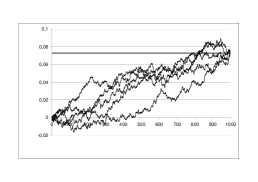
Figure 9: Trajectories in the normal
case for $P(\mathbf{S}_{1}^{n}>na)=10^{-2}$

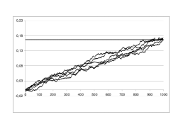
Figure 10: Trajectories in the normal
case for $P(\mathbf{S}_{1}^{n}>na)=10^{-8}$

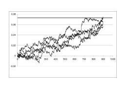
Figure 11: Trajectories in the expo-
nential case for $P(\mathbf{S}_{1}^{n}>na)=10^{-2}$

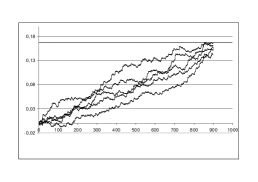
Figure 12: Trajectories in the expo-
nential case for $P(\mathbf{S}_{1}^{n}>na)=10^{-8}$

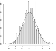
Figure 13: Distribution of $\textbf{X}_{i}^{\prime}s$ in the
normal case for $P(\mathbf{S}_{1}^{n}>na)=10^{-2}$

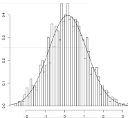
Figure 14: Distribution of $\textbf{X}_{i}^{\prime}s$ in the
normal case for $P(\mathbf{S}_{1}^{n}>na)=10^{-8}$

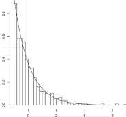
Figure 15: Distribution of $\textbf{X}_{i}^{\prime}s$ in the
exponential case for
$P(\mathbf{S}_{1}^{n}>na)=10^{-2}$

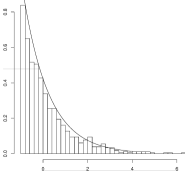
Figure 16: Distribution of $\textbf{X}_{i}^{\prime}s$ in the
exponential case for
$P(\mathbf{S}_{1}^{n}>na)=10^{-8}$

Consider now the case when $f(x)=x^{2}.$ Table 1 presents the case when $\mathbf{X}$ is $N(0,1)$, $n=1000,k=800$, $P\left(\mathbf{U}_{1}^{n}=n\left(a\sqrt{2}+1\right)\right)\simeq 10^{-2}.$ We present the histograms of the $X_{i}^{\prime}s$ together with the graph of the corresponding titlted density; when $\mathbf{X}$ is $N(0,1)$ then $\mathbf{X}^{2}$ is $\chi^{2}.$ It is well known that when $a$ is fixed larger than $1$ then the limit distribution of $\mathbf{X}_{1}$ conditioned on $\left(\mathbf{U}_{1}^{n}=n\left(a\sqrt{2}+1\right)\right)$ tends to $N\left(0,1+a\sqrt{2}\right)$ which is the Kullback-Leibler projection of $N(0,1)$ on the set of all probability measures $Q$ on $\mathbb{R}$ with $\int x^{2}dQ(x)=a\sqrt{2}+1.$ Now this distribution is precisely $h_{0}(\left.y_{1}\right|y_{0})$ defined hereabove. Also consider (22); expansion using the definitions (23) and (24) prove that as $n\rightarrow\infty$ the dominating term in $h_{i}(\left.y_{i+1}\right|y_{1}^{i})$ is precisely $N\left(0,1+a\sqrt{2}\right),$ and the terms including $y_{i+1}^{4}$ in the exponential stemming from $\mathfrak{n}\left(\alpha\beta+\left(\sigma a+\mu\right),\alpha,f(y_{i+1})\right)$ are of order $O\left(1/\left(n-i\right)\right)$; the terms depending on $y_{1}^{i}$ are of smaller order. The fit which is observed in Table 17 is in concordance with the above statement in the LDP range (fixed $a$), and with the MDP approximation following Ermakov; see [10] .

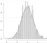
Figure 17: Distribution of $\textbf{X}_{i}^{\prime}s$ in the
normal case for $P(\mathbf{S}_{1}^{n}>na)=10^{-2}$
and for $f(x)=x^{2}$

Remark 11

The statistics $\mathbf{U}_{1}^{n}$ may be substituted by any regular M-estimator when $a=a_{n}$ defines a moderate deviation event, namely when (A) holds together with $a_{n}\rightarrow 0.$ In this case it is well known that the distribution of any regular $M$-estimator is similar to that of the mean of its influence function evaluated on the sample points; this allows to simulate samples under a given model conditionally on an observed value of a statistics, when observed in a rare area under the model.

5 Conclusion

We have obtained an extended version of Gibbs conditional principle in the simple case of real valued independent r.v’s conditioned on the value of their mean or on an average of their images through some real valued function. The approximation of the density of long runs is shown to be quite accurate and can be controlled through an explicit rule. Algorithms for the simulation of these runs are presented, together with numerical examples. Applications to Importance Sampling procedures for rare event simulation is a first application of this scheme; it mainly requires to consider conditioning events of the form $\left(\mathbf{S}_{1}^{n}>n\left(\sigma a_{n}+\mu\right)\right)$ instead of $\left(\mathbf{S}_{1}^{n}=n\left(\sigma a_{n}+\mu\right)\right)$; first numerical results obtained in [3] show a net gain in the variance for IS estimators using an extension of the present scheme. Extension to the multivariate setting is obtainable, requiring slight modifications. The case when the conditioning event is in the CLT zone deserves attention due to its interest to statistics. Simulation of $\mathbf{X}_{1}^{n}$ under a given $p_{\theta_{0}}$ in a model $\left(p_{\theta},\theta\in\Theta\right)$ may lead to conditional test when $a$ is substituted by the observed value of a given statistics. The present case when conditioning under a moderate deviation event is of interest for accurate assesment when the observed statistics has small $p-$ value under a given hypothesis. Some other potential application to statistics is related to test procedures in presence of nuisance parameter, considering conditional tests under a sufficient statistics for the nuisance.

Appendix A Three Lemmas pertaining to the partial sum under its final value

We state three lemmas which describe some functions of the random vector $\mathbf{X}_{1}^{n}$ conditioned on $\mathcal{E}_{n}$. The r.v. $\mathbf{X}$ is assumed to have expectation $0$ and variance $1.$

Lemma 12

It holds $E_{\mathfrak{P}_{n}}\left(\mathbf{X}_{1}\right)=a,E_{\mathfrak{P}_{n}}\left(\mathbf{X}_{1}\mathbf{X}_{2}\right)=a{}^{2}+0\left(\frac{1}{n}\right).$ $E_{\mathfrak{P}_{n}}\left(\mathbf{X}_{1}^{2}\right)=s^{2}(t)+a{}^{2}+0\left(\frac{1}{n}\right)$ where $m(t)=a.$

Proof. Using

$$\mathfrak{P}_{n}(\mathbf{X}_{1}=x)=\frac{p_{\mathbf{S}_{2}^{n}}\left(na-x\right)p_{\mathbf{X}_{1}}(x)}{p_{\mathbf{S}_{1}^{n}}\left(na\right)}=\frac{\pi_{\mathbf{S}_{2}^{n}}^{a}\left(na-x\right)\pi_{\mathbf{X}_{1}}^{a}(x)}{\pi_{\mathbf{S}_{1}^{n}}^{a}\left(na\right)}$$

normalizing both $\pi_{\mathbf{S}_{2}^{n}}^{a}\left(na-x\right)$ and $\pi_{\mathbf{S}_{1}^{n}}^{a}\left(na\right)$ and making use of a first order Edgeworth expansion in those expressions yields the asymptotic expressions for $E_{\mathfrak{P}_{n}}\left(\mathbf{X}_{1}^{2}\right)=s^{2}(t)+a{}^{2}+0\left(\frac{1}{n}\right)$ here above.   A similar development for the joint density $\mathfrak{P}_{n}(\mathbf{X}_{1}=x,\mathbf{X}_{2}=y)$, using the same tilted distribution $\pi^{a}$ it readily follows that the last result holds. We used the fact that $a_{n}$ is a bounded sequence.   

The following result states the behavior of the moments of $\pi^{m_{i}}.$

Lemma 13

Assume (A) and (E1). Then $\max_{1\leq i\leq k}\left|m_{i}\right|=a+o_{\mathfrak{P}_{n}}\left(\epsilon_{n}\right).$ Also $\max_{1\leq i\leq k}s_{i}^{2}$, $\max_{1\leq i\leq k}\mu_{3}^{i}$ and $\max_{1\leq i\leq k}\mu_{4}^{i}$ tend in $\mathfrak{P}_{n}$ probability to the variance, skewness and kurtosis of $p$ when $a=a_{n}\rightarrow 0$ and remain bounded when $a$ is fixed positive.

Proof. Define

$$V_{i+1} :=m(t_{i})-a$$

$$=\frac{\Sigma_{i+1}^{n}}{n-i}-a.$$

We state that

$${\max_{0\leq{i\leq{k-1}}}|V_{i+1}|=}o_{\mathfrak{P}_{n}}\left(\epsilon_{n}\right),$$ (36)

namely for all positive $\delta$

$$\lim_{n\rightarrow\infty}\mathfrak{P}_{n}\left(\max_{0\leq{i\leq{k-1}}}|V_{i+1}|>\delta\epsilon_{n}\right)=0$$

which we prove following Kolmogorov maximal inequality. Define

$$A_{i}:=\left(\left(|V_{i+1}|\geq\delta\epsilon_{n}\right)\text{ and }\left(|V_{j}|<\delta\epsilon_{n}\text{ for all }j<i+1\right)\right).$$

from which

$$\left(\max_{0\leq{i}\leq{k-1}}|V_{i+1}|>\delta\epsilon_{n}\right)=\bigcup_{i=0}^{k-1}A_{i}.$$

It holds

$$E_{\mathfrak{P}_{n}}V_{k}^{2} ={\int_{\cup A_{i}}V_{k}^{2}d\mathfrak{P}_{n}+\int_{\left(\cup A_{i}\right)^{c}}V_{k}^{2}d}\mathfrak{P}_{n}$$

$$\geq{\int_{\cup A_{i}}}\left({V_{i}^{2}+2}\left(V_{k}-V_{i}\right)V_{i}\right){d\mathfrak{P}_{n}+\int_{\left(\cup A_{i}\right)^{c}}}\left({V_{i}^{2}+2}\left(V_{k}-V_{i}\right)V_{i}\right){d}\mathfrak{P}_{n}$$

$$\geq{\int_{\cup A_{i}}V_{i}^{2}d}\mathfrak{P}_{n}$$

$$\geq\delta^{2}\epsilon_{n}^{2}{\sum_{j=0}^{k-1}\mathfrak{P}_{n}(A_{j})}$$

$$=\delta^{2}\epsilon_{n}^{2}\mathfrak{P}_{n}\left({\max_{0\leq{i}\leq{k-1}}|V_{i+1}|>}\delta\epsilon_{n}\right).$$

The third line above follows from $EV_{i}\left(V_{k}-V_{i}\right)=0$ which is proved hereunder. Hence

$$\mathfrak{P}_{n}\left({\max_{0\leq{i}\leq{k-1}}|V_{i+1}|>}\delta\epsilon_{n}\right)\leq\frac{Var_{\mathfrak{P}_{n}}(V_{k})}{\delta^{2}\epsilon_{n}^{2}}=\frac{1}{\delta^{2}\epsilon_{n}^{2}\left(n-k\right)}(1+o(1))$$

where we used Lemma 12; therefore (36) holds under (E1). By direct calculation, we can show that $E_{\mathfrak{P}_{n}}\left(V_{i}(V_{k}-V_{i})\right)={0}$, which achieves the proof.   

We also need the order of magnitude of $\max\left(\mathbf{X}_{1},...,\mathbf{X}_{k}\right)$ under $\mathfrak{P}_{n}$ which is stated in the following result.

Lemma 14

For all $k$ between $1$ and $n,\max\left(\mathbf{X}_{1},...,\mathbf{X}_{k}\right)=O_{\mathfrak{P}_{n}}\left(\log k\right).$

Proof. For all $t$ it holds

$$\mathfrak{P}_{n}\left(\max\left(\mathbf{X}_{1},...,\mathbf{X}_{k}\right)>t\right) \leq k\mathfrak{P}_{n}\left(\mathbf{X}_{n}>t\right)$$

$$=k\int_{t}^{\infty}\pi^{a}\left(\mathbf{X}_{n}=u\right)\frac{\pi^{a}(\mathbf{S}_{1}^{n-1}=na_{n}-u)}{\pi^{a}\left(\mathbf{S}_{1}^{n}=na_{n}\right)}du.$$

Let $\tau$ be such that $m(\tau)=a.$ Center and normalize both $\mathbf{S}_{1}^{n}$ and $\mathbf{S}_{1}^{n-1}$with respect to the density $\pi^{a}$ in the last line above, denoting $\overline{\pi_{n}^{a}}$ the density of $\overline{\mathbf{S}_{1}^{n}}:=\left(\mathbf{S}_{1}^{n}-na_{n}\right)/s^{(a)}\sqrt{n}$ when $\mathbf{X}$ has density $\pi^{a}$ with mean $a$ and variance $\left(s^{(a)}\right)^{2},$ we get

$$\mathfrak{P}_{n}\left(\max\left(\mathbf{X}_{1},...,\mathbf{X}_{k}\right)>t\right) \leq k\frac{\sqrt{n}}{\sqrt{n-1}}\int_{t}^{\infty}\pi^{a}\left(\mathbf{X}_{n}=u\right)$$

$$\frac{\overline{\pi_{n-1}^{a}}\left(\overline{\mathbf{S}_{1}^{n-1}}=\left(na-u-(n-1)a\right)/\left(s^{(a)}\sqrt{n-1}\right)\right)}{\overline{\pi_{n}^{a}}\left(\overline{\mathbf{S}_{1}^{n}}=0\right)}du.$$

Under the sequence of densities $\pi^{a}$ the triangular array $\left(\mathbf{X}_{1},...,\mathbf{X}_{n}\right)$ obeys a first order Edgeworth expansion

$$\mathfrak{P}_{n}\left(\max\left(\mathbf{X}_{1},...,\mathbf{X}_{k}\right)>t\right) \leq k\frac{\sqrt{n}}{\sqrt{n-1}}\int_{t}^{\infty}\pi^{a}\left(\mathbf{X}_{n}=u\right)$$

$$\frac{\mathfrak{n}\left(\left(a-u\right)/s^{(a)}\sqrt{n-1}\right)\mathbf{P}\left(u,i,n\right)+o(1)}{\mathfrak{n}\left(0\right)+o(1)}du$$

$$\leq kCst\int_{t}^{\infty}\pi^{a}\left(\mathbf{X}_{n}=u\right)du.$$

for some constant $Cst$ independent of $n$ and $\tau$ and

$$\mathbf{P}\left(u,i,n\right):=1+P_{3}\left(\left(a-u\right)/s^{(a)}\sqrt{n-1}\right)$$

where $P_{3}(x)=\frac{\mu_{3}^{(a)}}{6\left(s^{(a)}\right)^{3}}\left(x^{3}-3x\right)$ is the third Hermite polynomial; $\mu_{3}^{(a)}$ is the third centered moment of $\pi^{a}.$ We used uniformity upon $u$ in the remaining term of the Edgeworth expansions. Making use of Chernoff Inequality to bound $\Pi^{a}\left(\mathbf{X}_{n}>t\right),$

$$\mathfrak{P}_{n}\left(\max\left(\mathbf{X}_{1},...,\mathbf{X}_{k}\right)>t\right)\leq kCst\frac{\Phi(t+\lambda)}{\Phi(t)}e^{-\lambda t}$$

for any $\lambda$ such that $\phi(t+\lambda)$ is finite. For $t$ such that

$$t/\log k\rightarrow\infty$$

it holds

$$\mathfrak{P}_{n}\left(\max\left(\mathbf{X}_{1},...,\mathbf{X}_{k}\right)<t\right)\rightarrow 1,$$

which proves the lemma.

 

Appendix B Proof of the approximations resulting from Edgeworth expansions in Theorem 1

We complete the calculation leading to (15) and (16).

Set $Z_{i+1}:=\left(m_{i}-Y_{i+1}\right)/s_{i}\sqrt{n-i-1}.$

It then holds

$$\overline{\pi_{n-i-1}}\left(Z_{i+1}\right) =\mathfrak{n}(Z_{i+1})\left[\begin{array}[]{c}1+\frac{1}{\sqrt{n-i-1}}P_{3}(Z_{i+1})+\frac{1}{n-i-1}P_{4}(Z_{i+1})\\ +\frac{1}{\left(n-i-1\right)^{3/2}}P_{5}(Z_{i+1})\end{array}\right]$$ (39)

$$+O_{\mathfrak{P}_{n}}\left(\frac{1}{\left(n-i-1\right)^{3/2}}\right).$$

We perform an expansion in $\mathfrak{n}(Z_{i+1})$ up to the order $3,$ with a first order term $\mathfrak{n}\left(-Y_{i+1}/\left(s_{i}\sqrt{n-i-1}\right)\right),$ namely

$$\mathfrak{n}(Z_{i+1}) =\mathfrak{n}\left(-Y_{i+1}/\left(s_{i}\sqrt{n-i-1}\right)\right)$$ (40)

$$\left(\begin{array}[]{c}1+\frac{Y_{i+1}m_{i}}{s_{i}^{2}\left(n-i-1\right)}+\frac{m_{i}^{2}}{2s_{i}^{2}\left(n-i-1\right)}\left(\frac{Y_{i+1}^{2}}{s_{i}^{2}\left(n-i-1\right)}-1\right)\\ +\frac{m_{i}^{3}}{6s_{i}^{3}\left(n-i-1\right)^{3/2}}\frac{\mathfrak{n}^{(3)}\left(\frac{Y^{\ast}}{\left(s_{i}\sqrt{n-i-1}\right)}\right)}{\mathfrak{n}\left(-Y_{i+1}/\left(s_{i}\sqrt{n-i-1}\right)\right)}\end{array}\right)$$ (43)

where $Y^{\ast}=\frac{1}{s_{i}\sqrt{n-i-1}}(-Y_{i+1}+\theta m_{i})$ with $\left|\theta\right|<1.$

Lemmas 13 and 14 provide the orders of magnitude of the random terms in the above displays when sampling under $\mathfrak{P}_{n}.$

Use those lemmas to obtain

$$\frac{Y_{i+1}m_{i}}{s_{i}^{2}\left(n-i-1\right)}=\frac{Y_{i+1}}{n-i-1}\left(a+o_{\mathfrak{P}_{n}}\left(\epsilon_{n}\right)\right)$$ (44)

and

$$\frac{m_{i}^{2}}{s_{i}^{2}\left(n-i-1\right)}=\frac{1}{n-i-1}\left(a+o_{\mathfrak{P}_{n}}\left(\epsilon_{n}\right)\right)^{2}.$$

Also when (A) holds then the dominant terms in the bracket in (40) are precisely those in the two displays just above. This yields

$$\mathfrak{n}(Z_{i+1})=\mathfrak{n}\left(\frac{-Y_{i+1}}{s_{i}\sqrt{n-i-1}}\right)\left(\begin{array}[]{c}1+\frac{aY_{i+1}}{s_{i}^{2}(n-i-1)}-\frac{a^{2}}{2s_{i}^{2}(n-i-1)}\\ +\frac{o_{\mathfrak{P}_{n}}(\epsilon_{n}\log n)}{n-i-1}\end{array}\right).$$

We now need a precise evaluation of the terms in the Hermite polynomials in (39). This is achieved using Lemmas 13 and 14 which provide uniformity upon $i$ between $1$ and $k=k_{n}$ in all terms depending on the sample path $Y_{1}^{k}.$ The Hermite polynomials depend upon the moments of the underlying density $\pi^{m_{i}}.$ Since $\overline{\pi_{1}^{m_{i}}}$ has expectation $0$ and variance $1$ the terms corresponding to $P_{1}$  and $P_{2}$ vanish. Up to the order $4$ the polynomials write $P_{3}(x)=\frac{\mu_{3}^{(i)}}{6\left(s_{i}\right)^{3}}H_{3}(x)$, $P_{4}(x)=\frac{(\mu_{3}^{i})^{2}}{72\left(s_{i}\right)^{6}}H_{6}(x)+\frac{\mu_{4}^{(i,n)}-3\left(s_{i}\right)^{4}}{24\left(s_{i}\right)^{4}}H_{4}(x)$ with $H_{3}(x):=x^{3}-3x$, $H_{4}(x):=x^{4}+6x^{2}-3$ and $H_{6}(x):=x^{6}-15x^{4}+45x^{2}-15.$

Using Lemma 13 it appears that the terms in $x^{j},$ $j\geq 3$ in $P_{3}$ and $P_{4}$ will play no role in the asymptotic behavior in (39) with respect to the constant term in $P_{4}$ and the term in $x$ from $P_{3}\ .$ Indeed substituting $x$ by $Z_{i+1}$ and dividing by $n-i-1$, the term in $x^{2}$ in $P_{4}$ writes $O_{\mathfrak{P}_{n}}\left(\log n\right)^{2}/(n-i)^{2}$ where we used Lemma 13. These terms are of smaller order than the term $-3x$ in $P_{3}$ which writes $-\frac{\mu_{3}^{i}}{2s_{i}^{4}\left(n-i-1\right)}\left(a-Y_{i+1}\right)=\frac{1}{n-i-1}O_{\mathfrak{P}_{n}}\left(\log n\right).$

It holds

$$\frac{P_{3}(Z_{i+1})}{\sqrt{n-i-1}} =-\frac{\mu_{3}^{i}}{2s_{i}^{4}\left(n-i-1\right)}\left(m_{i}-Y_{i+1}\right)$$

$$\text{ }+\frac{\mu_{3}^{i}\left(m_{i}-Y_{i+1}\right)^{3}}{6\left(s_{i}\right)^{6}(n-i-1)^{2}}$$

which yields

$$\frac{P_{3}(Z_{i+1})}{\sqrt{n-i-1}}=-\frac{\mu_{3}^{i}}{2s_{i}^{4}\left(n-i-1\right)}\left(a-Y_{i+1}\right)+\frac{1}{\left(n-i-1\right)^{2}}O_{\mathfrak{P}_{n}}\left(\log n\right)^{3}.$$ (45)

For the term of order $4$ it holds

$$\frac{P_{4}(Z_{i+1})}{n-i-1}=\frac{1}{n-i-1}\left(\frac{(\mu_{3}^{i})^{2}}{72s_{i}^{6}}H_{6}(Z_{i+1})+\frac{\mu_{4}^{i}-3s_{i}^{4}}{24s_{i}^{4}}H_{4}(Z_{i+1})\right)$$

which yields

$$\frac{P_{4}(Z_{i+1})}{n-i-1}=-\frac{\mu_{4}^{i}-3s_{i}^{4}}{8s_{i}^{4}\left(n-i-1\right)}-\frac{15(\mu_{3}^{i})^{2}}{72s_{i}^{6}(n-i-1)}+\frac{O_{\mathfrak{P}_{n}}\left((\log n)^{2}\right)}{\left(n-i-1\right)^{2}}.$$ (46)

The fifth term in the expansion plays no role in the asymptotics, under (A).

To sum up , under (A), and comparing the remainder terms in (45) and (46), we get

$$\overline{\pi_{n-i-1}}\left(Z_{i+1}\right)=\mathfrak{n}\left(-Y_{i+1}/\left(s_{i}\sqrt{n-i-1}\right)\right).A.B+O_{\mathfrak{P}_{n}}\left(\frac{1}{\left(n-i-1\right)^{3/2}}\right)$$

where $A$ and $B$ are given in (15) and (16).

Appendix C Final step of the proof of Theorem 1

We make use of the following version of the law of large numbers for triangular arrays (see [14] Theorem 3.1.3).

Theorem 15

Let $X_{i,n}$ ,$1\leq i\leq k$ denote an array of row-wise real exchangeable r.v’s and $\lim_{n\rightarrow\infty}k=\infty.$ Let $\rho_{n}:=EX_{1,n}X_{2,n}.$ Assume that for some finite $\Gamma$ , $EX_{1,n}^{2}\leq\Gamma.$ If for some doubly indexed sequence $\left(a_{i,n}\right)$ such that $\lim_{n\rightarrow\infty}\sum_{i=1}^{k}a_{i,n}^{2}=0$ it holds

$$\lim_{n\rightarrow\infty}\rho_{n}\left(\sum_{i=1}^{k}a_{i,n}^{2}\right)^{2}=0$$

then

$$\lim_{n\rightarrow\infty}\sum_{i=1}^{k}a_{i,n}X_{i,n}=0$$

in probability.

Denote

$$\kappa_{1}^{i}:=\frac{\mu_{3}^{i}}{2s_{i}^{4}}\text{ \ \ , \ \ }\kappa_{2}^{i}:=\frac{\mu_{3}^{i}-s_{i}^{4}}{8s_{i}^{4}}+\frac{15(\mu_{3}^{i})^{2}}{72s_{i}^{6}},$$

$$\mu_{1}^{\ast}:=\kappa_{1}^{i}+\frac{a}{s_{i}^{2}}\text{ \ \ , \ \ }\mu_{2}^{\ast}:=\kappa_{1}^{i}-\frac{a}{2s_{i}^{2}}.$$

By (13), (14) and (17)

$$p(\mathbf{X}_{i+1}=Y_{i+1}|S_{i+1}^{n}=na_{n}-\Sigma_{1}^{i})=\frac{\sqrt{n-i}}{\sqrt{n-i-1}}\pi^{m_{i}}\left(\mathbf{X}_{i+1}=Y_{i+1}\right)\frac{\mathfrak{n}\left(\frac{-Y_{i+1}}{s_{i}\sqrt{n-i-1}}\right)}{\mathfrak{n}(0)}A(i)$$

with

$$A(i):=\frac{1+\frac{\mu_{1}^{\ast}Y_{i+1}}{n-i-1}-\frac{\mu_{2}^{\ast}a}{n-i-1}-\frac{\kappa_{2}^{i}}{n-i-1}+\frac{o_{\mathfrak{P}_{n}}\left(\epsilon_{n}\log n\right)}{n-i-1}}{1-\frac{\kappa_{2}^{i}}{n-i}+O_{\mathfrak{P}_{n}}\left(\frac{1}{(n-i)^{3/2}}\right)}.$$

We perform a second order expansion in both the numerator and the denominator of the above expression, which yields

$$A(i)=\exp\left(\frac{\mu_{1}^{\ast}Y_{i+1}}{n-i-1}-\frac{a}{2s_{i}^{2}(n-i-1)}\right)\exp\left(-\frac{a\kappa_{1}^{i}}{n-i-1}\right)\exp\left(\frac{o_{\mathfrak{P}_{n}}\left(\epsilon_{n}\log n\right)}{n-i-1}\right)A^{\prime}(i).$$ (47)

The term $\exp\left(\frac{\mu_{1}^{\ast}Y_{i+1}}{n-i-1}+\frac{a}{2s_{i}^{2}(n-i-1)}\right)$ in (47) is captured in $g_{i}(\left.Y_{i+1}\right|Y_{1}^{i}).$

The term $A^{\prime}(i)$ in (47) writes

$$A^{\prime}(i):=Q_{1}^{i}.Q_{2}^{i}$$

with

$$Q_{1}^{i}:=\exp\left(-\left(\begin{array}[]{c}\frac{\kappa_{2}^{i}}{(n-i-1)(n-i)}+\frac{(\kappa_{2}^{i})^{2}}{2(n-i)^{2}}+\frac{1}{2}\left(\frac{\mu_{1}^{\ast}Y_{i+1}}{n-i-1}-\frac{a\mu_{2}^{\ast}}{n-i-1}-\frac{\kappa_{2}^{i}}{n-i-1}\right)^{2}\end{array}\right)\right)$$

and

$$Q_{2}^{i}:=\frac{\exp B_{1}}{\exp B_{2}}$$

where

$$B_{1} :=\frac{o_{\mathfrak{P}_{n}}(\epsilon_{n}^{2}(\log n)^{2})}{(n-i-1)^{2}}+\frac{\mu_{1}^{\ast}Y_{i+1}}{(n-i-1)^{2}}o_{\mathfrak{P}_{n}}\left(\epsilon_{n}\log n\right)$$

$$+\frac{\mu_{2}^{\ast}a}{(n-i-1)^{2}}o_{\mathfrak{P}_{n}}(\epsilon_{n}\log n)+\frac{o_{\mathfrak{P}_{n}}(\epsilon_{n}^{2}\left(\log n)\right)^{2}}{(n-i-1)^{2}}+o(u_{1}^{2})$$

$$B_{2}:=\frac{\kappa_{2}^{i}}{n-i}O_{\mathfrak{P}_{n}}\left(\frac{1}{(n-i)^{3/2}}\right)+O_{\mathfrak{P}_{n}}\left(\frac{1}{(n-i)^{3}}\right)+$$

$$O_{\mathfrak{P}_{n}}\left(\frac{1}{(n-i)^{3/2}}\right)+o\left(\left(\frac{\kappa_{2}^{i}}{n-i}+O_{\mathfrak{P}_{n}}\left(\frac{1}{(n-i)^{3/2}}\right)\right)^{2}\right).$$

with

$$u_{1}=\frac{\mu_{1}^{\ast}Y_{i+1}}{n-i-1}-\frac{\mu_{2}^{\ast}a}{n-i-1}-\frac{\kappa_{2}^{i}}{n-i-1}+\frac{o_{\mathfrak{P}_{n}}(\epsilon_{n}\log n)}{n-i-1}.$$

We first prove that

$$\prod\limits_{i=0}^{k-1}A^{\prime}(i)=1+o_{\mathfrak{P}_{n}}(\epsilon_{n}\left(\log n\right)^{2})$$ (48)

as $n$ tends to infinity.

Since

$$p(\mathbf{X}_{1}^{k}=Y_{1}^{k}|S_{i+1}^{n}=na_{n})=\prod\limits_{i=0}^{k-1}g_{i}\left(\left.Y_{i+1}\right|Y_{1}^{i}\right)\prod\limits_{i=0}^{k-1}A^{\prime}(i)\prod\limits_{i=0}^{k-1}L_{i}$$

where

$$L_{i}:=\frac{C_{i}^{-1}}{\Phi\left(t_{i}\right)}\frac{\sqrt{n-i}}{\sqrt{n-i-1}}\exp\left(-\frac{a\kappa_{1}^{i}}{n-i-1}\right)$$

the  completion of the proof will follow from

$$\prod\limits_{i=0}^{k-1}L_{i}=1+o_{\mathfrak{P}_{n}}(\epsilon_{n}\left(\log n\right)^{2}).$$ (49)

The proof of (48) is achieved in two steps.

Claim 16

$\prod_{i=0}^{k-1}Q_{1}^{i}=1+o_{\mathfrak{P}_{n}}(\epsilon_{n}\left(\log n\right)^{2}).$

By Lemma 13 the random terms $\mu_{j}^{i}$ deriving from $\pi^{m_{i}}$ satisfy

$$max_{1\leq i\leq k}\left|\mu_{j}^{i}-\mu_{j}\right|=o_{\mathfrak{P}_{n}}(1)$$

as $n$ tends to $\infty,$ where $\mu_{j}$ is the $j$-th centered moment of $p.$ Therefore we may substitute $\mu_{j}^{i}$ by $\mu_{j}$ in order to check the convergence of all subsequent series.

Developing $Q1,$ define, for any positive $\beta_{1}$, $\beta_{2}$, $\beta_{3}$ and $\beta_{4}$

$$A_{n}^{1}:=\left\{\frac{1}{\epsilon_{n}\left(\log n\right)^{2}}\sum_{i=0}^{k-1}\left|\frac{\kappa_{2}^{i}}{(n-i-1)(n-i)}\right|<\beta_{1}\right\},$$

$$A_{n}^{2}:=\left\{\frac{1}{\epsilon_{n}\left(\log n\right)^{2}}\sum_{i=0}^{k-1}\left|\frac{(\kappa_{2}^{i})^{2}}{(n-i-1)^{2}}\right|<\beta_{2}\right\},$$

$$A_{n}^{3}:=\left\{\frac{1}{\epsilon_{n}\left(\log n\right)^{2}}\sum_{i=0}^{k-1}\left|\frac{(\mu_{2}^{\ast}a)^{2}}{(n-i-1)^{2}}\right|<\beta_{3}\right\}$$

and

$$A_{n}^{4}:=\left\{\frac{1}{\epsilon_{n}\left(\log n\right)^{2}}\sum_{i=0}^{k-1}\left|\frac{\mu_{2}^{\ast}\kappa_{2}^{i}a}{(n-i-1)^{2}}\right|<\beta_{4}\right\}.$$

It clearly holds that

$$\lim_{n\rightarrow\infty}\mathfrak{P}_{n}\left(A_{n}^{j}\right)=1;\text{ }j=1,...,4.$$

Let for any positive $\beta_{5}$

$$A_{n}^{5}:=\left\{\frac{1}{\epsilon_{n}\left(\log n\right)^{2}}\sum_{i=0}^{k-1}\left|\frac{\kappa_{1}^{i}\kappa_{2}^{i}Y_{i+1}}{(n-i-1)^{2}}\right|<\beta_{5}\right\}.$$

If $\lim_{n\rightarrow\infty}\mathfrak{P}_{n}\left(A_{n}^{5}\right)=1$, then $\lim_{n\rightarrow\infty}\mathfrak{P}_{n}\left(A_{n}^{j}\right),$ $j=6,7$ where

$$A_{n}^{6}:=\left\{\frac{1}{\epsilon_{n}\left(\log n\right)^{2}}\sum_{i=0}^{k-1}\left|\frac{\mu_{1}^{\ast}\kappa_{2}^{i}Y_{i+1}}{(n-i-1)^{2}}\right|<\beta_{6}\right\}$$

$$A_{n}^{7}:=\left\{\frac{1}{\epsilon_{n}\left(\log n\right)^{2}}\sum_{i=0}^{k-1}\left|\frac{\mu_{1}^{\ast}\mu_{2}^{\ast}aY_{i+1}}{(n-i-1)^{2}}\right|<\beta_{7}\right\}.$$

Apply Theorem 15 with $X_{i,n}=Y_{i+1}$ and $a_{i,n}=\frac{1}{\epsilon_{n}\left(\log n\right)^{2}(n-i-1)^{2}}.$ By Lemma 12

$$E_{\mathfrak{P}_{n}}Y_{1}^{2}=s^{2}(0)+a+O\left(\frac{1}{n}\right).$$

Hence $E_{\mathfrak{P}_{n}}[Y_{1}^{2}]\leq{\Gamma}$ for some finite $\Gamma.$ Further $\rho_{n}=a^{2}+O\left(\frac{1}{n}\right).$ Both conditions in Theorem 15 are fullfilled. Indeed

$$\lim_{n\rightarrow\infty}\sum_{i=1}^{k}a_{n,i}^{2}=\lim_{n\rightarrow\infty}\frac{1}{\epsilon_{n}^{2}\left(\log n\right)^{4}(n-k)^{3}}=0$$

which holds under (E1), as holds

$$\lim_{n\rightarrow\infty}\rho_{n}\left(\sum_{i=1}^{k}a_{n,i}\right)^{2}=\lim_{n\rightarrow\infty}\frac{a^{2}}{\epsilon_{n}^{2}\left(\log n\right)^{4}(n-k)^{2}}=0.$$

Therefore, for i between $5$ and $7$, we have

$$\lim_{n\rightarrow\infty}\mathfrak{P}_{n}\left(A_{n}^{i}\right)=1.$$

Define for any positive $\beta_{8}$

$$A_{n}^{8}:=\left\{\frac{1}{\epsilon_{n}\left(\log n\right)^{2}}\sum_{i=0}^{k-1}\frac{\left(\mu_{1}^{\ast}\right)^{2}Y_{i+1}^{2}}{(n-i-1)^{2}}<\beta_{8}\right\}.$$

Apply Theorem 15 with $X_{i,n}=Y_{i+1}^{2}$ and $a_{i,n}=\frac{1}{\epsilon_{n}\left(\log n\right)^{2}(n-i-1)^{2}}.$

It holds

$$\lim_{n\rightarrow\infty}\sum_{i=1}^{k}a_{n,i}^{2}=0$$

when (E1) holds.

By Lemma 12,

$$E_{\mathfrak{P}_{n}}Y_{1}^{4}=E_{\pi^{a}}Y_{1}^{4}+O\left(\frac{1}{n}\right)$$

which entails that for some positive constant $\Gamma$   such that $EY_{1}^{4}\leq{\Gamma}<\infty.$ Also

$$E_{\mathfrak{P}_{n}}\left(Y_{1}^{2}Y_{2}^{2}\right)=\left(s^{2}(0)+a\right)\left(s^{2}(0)+a\right)+O\left(\frac{1}{n}\right)$$

and

$$\lim_{n\rightarrow\infty}\rho_{n}\left(\frac{1}{\epsilon_{n}\left(\log n\right)^{2}}\sum_{i=0}^{k-1}\frac{1}{(n-i-1)^{2}}\right)^{2}=0$$

which holds under (E1). Hence

$$\lim_{n\rightarrow\infty}\mathfrak{P}_{n}\left(A_{n}^{8}\right)=1.$$

It follows that, noting $A_{n}$ the intersection of the events $A_{n}^{i}$ , $j=1,...,8$

$$\lim_{n\rightarrow\infty}\mathfrak{P}_{n}\left(A_{n}\right)=1.$$

To sum up, we have proved that, under (E1),

$$Q1=1+o_{\mathfrak{P}_{n}}\left(\epsilon_{n}\left(\log n\right)^{2}\right).$$

Claim 17

$\prod_{i=0}^{k-1}Q_{2}^{i}=1+o_{\mathfrak{P}_{n}}\left(\epsilon_{n}\left(\log n\right)^{2}\right).$

This amounts to prove that the sum of the terms in $B1$ (resp in $B2$) is of order $o_{\mathfrak{P}_{n}}\left(\epsilon_{n}\left(\log n\right)^{2}\right).$

The four terms in the the sum of the terms in $B1$ are respectively of order $o_{\mathfrak{P}_{n}}\left(\epsilon_{n}^{2}(\log n)^{4}\right)/(n-k)$, $o_{\mathfrak{P}_{n}}\left(\epsilon_{n}(\log n)^{3}\right)/(n-k),$ $o_{\mathfrak{P}_{n}}\left(a\epsilon_{n}(\log n)^{2}\right)/(n-k)$ and $o_{\mathfrak{P}_{n}}\left(\epsilon_{n}(\log n)^{2}\right)/(n-k)$ using Lemma 13. The sum of the terms $o\left(u_{1}^{2}\right)$ is of order less than those ones. Assuming (E1) all those terms are $o_{\mathfrak{P}_{n}}\left(\epsilon_{n}\left(\log n\right)^{2}\right).$

For the sum of terms $B2$, by uniformity of the Edgeworth expansion with respect to $Y_{1}^{k}$ it holds $\sum_{i=1}^{k}B2=O_{\mathfrak{P}_{n}}\left(\left(n-k\right)^{-1/2}\right)$ which is $o_{\mathfrak{P}_{n}}\left(\epsilon_{n}\left(\log n\right)^{2}\right)$ by (E1).

We now turn to the proof of (49)

Define

$$u:=-x\frac{\mu_{3}^{i}}{2s_{i}^{4}\left(n-i-1\right)}+\frac{(x-a)^{2}}{2s_{i}^{2}\left(n-i-1\right)}.$$

Use the classical bounds

$$1-u+\frac{u^{2}}{2}-\frac{u^{3}}{6}\leq e^{-u}\leq 1-u+\frac{u^{2}}{2}$$

to obtain on both sides of the above inequalities the second order approximation of $C_{i}^{-1}$ through integration with respect to $p.$ The upper bound yields

$$C_{i}^{-1} \leq\Phi(t_{i})+\frac{\kappa_{1}^{i}}{n-i-1}\Phi^{\prime}(t_{i})+\frac{1}{s_{i}^{2}(n-i-1)}\left(\Phi"(t_{i})-2a\Phi^{\prime}\left(t_{i}\right)+a^{2}\right)$$

$$+O_{\mathfrak{P}_{n}}\left(\frac{1}{(n-i-1)^{2}}\right)$$

from which

$$L_{i}\leq\frac{\sqrt{n-i}}{\sqrt{n-i-1}}\exp\left(-\frac{a\kappa_{1}^{i}}{n-i-1}\right)\left(\begin{array}[]{c}1+\frac{\kappa_{1}^{i}}{n-i-1}m_{i}\\ -\frac{s_{i}^{2}+m_{i}^{2}-2am_{i}+a^{2}}{2s_{i}^{2}\left(n-i-1\right)}+O_{\mathfrak{P}_{n}}\left(\frac{1}{\left(n-i-1\right)^{2}}\right)\end{array}\right)$$

where the approximation term is uniform on the $Y_{1}^{k}.$

Subsituting $\frac{\sqrt{n-i}}{\sqrt{n-i-1}}$ and $\exp\left(-\frac{a\kappa_{1}^{i}}{n-i-1}\right)$ by their expansion $1+\frac{1}{2\left(n-i-1\right)}+O\left(\frac{1}{\left(n-i-1\right)^{2}}\right)$ and $1-\frac{a\kappa_{1}^{i}}{n-i-1}+\frac{(a\kappa_{1}^{i})^{2}}{(n-i-1)^{2}}+O\left(\frac{a^{2}}{(n-i-1)^{2}}\right)$ in the upper bound of $L_{i}$  above yields

$$L_{i} \leq\ \left(1+\frac{1}{2(n-i-1)}-\frac{a\kappa_{1}^{i}}{n-i-1}+\frac{(a\kappa_{1}^{i})^{2}}{2(n-i-1)^{2}}+o\left(\frac{1}{(n-i-1)^{2}}\right)\right)$$

$$\left(1+\frac{\kappa_{1}^{i}m_{i}}{n-i-1}-\frac{s_{i}^{2}+m_{i}^{2}-2am_{i}+a^{2}}{2s_{i}^{2}(n-i-1)}+O_{\mathfrak{P}_{n}}\left(\frac{1}{(n-i-1)^{2}}\right)\right).$$

Using Lemma 13, $m_{i}^{2}-2am_{i}+a^{2}=o_{\mathfrak{P}_{n}}(a\epsilon_{n})$ and therefore

$$L_{i} \leq\ \left(1+\frac{1}{2(n-i-1)}-\frac{a\kappa_{1}^{i}}{n-i-1}+\frac{(a\kappa_{1}^{i})^{2}}{(n-i-1)^{2}}+o\left(\frac{1}{(n-i-1)^{2}}\right)\right)$$

$$\left(1+\frac{\kappa_{1}^{i}a}{n-i-1}-\frac{1}{2(n-i-1)}+\frac{o_{\mathfrak{P}_{n}}(a\epsilon_{n})}{n-i-1}\right).$$

Write

$$\prod_{i=1}^{k}L_{i}\leq{\prod_{i=1}^{k}}\left({1+M_{i}}\right)$$

with

$$M_{i}=\frac{(a\kappa_{1}^{i})^{2}}{(n-i-1)^{2}}+\frac{o_{\mathfrak{P}_{n}}(a\epsilon_{n})}{n-i-1}.$$

Under (A) and (E1), $\sum_{i=0}^{k-1}M_{i}$ is $o_{\mathfrak{P}_{n}}\left(\epsilon_{n}\left(\log n\right)^{2}\right).$ This closes the proof of the Theorem.

References

• [1] Barbe, P. and Broniatowski, M. (1999). Simulation in exponential families. ACM Transactions on Modeling and Computer Simulation (TOMACS) 9 203–223.
• [2] Barndorff-Nielsen, O.(1978). Information and exponential families in statistical theory. Wiley Series in Probability and Mathematical Statistics. Chichester: John Wiley & Sons.
• [3] Broniatowski, M. and Ritov, Y. (2009) Importance Sampling for rare events and conditioned random walks. arXiv:0910.1819,2009
• [4] CsiszΓ‘r, I.(1984). Sanov property, generalized $I$-projection and a conditional limit theorem. Ann. Probab. 12 768–793.
• [5] Dembo, A. and Zetouni, O. (1996) Refinements of the Gibbs conditioning principle. Probab. Theory Related Fields 104 1–14.
• [6] den Hollander, W.Th.F. and Weiss, G.H. (1988) On the range of a constrained random walk. J. Appl. Probab. 25 451–463.
• [7] den Hollander, W.Th.F. and Weiss, G.H. (1988) A note on configurational properties of constrained random walks. J. Phys. A 21 2405–2415.
• [8] Diaconis, P. and Freedman, D.A. (1988) Conditional limit theorems for exponential families and finite versions of de Finetti’s theorem. J. Theoret. Probab. 1 381–410.
• [9] Dupuis, P. and Wang, H. (2004) Importance sampling, large deviations, and differential games. Stoch. Stoch. Rep. 76 481–508.
• [10] Ermakov, M.S. (2006) The importance sampling method for modeling the probabilities of moderate and large deviations of estimates and tests. Teor. Veroyatn. Primen. 51 319–332.
• [11] Feller, W. (1971) An introduction to probability theory and its applications. Vol.II. Second edition, John Wiley & Sons Inc., New York.
• [12] Jensen, J.L. (1995) Saddlepoint approximations. Oxford Statistical Science Series, 16. The Clarendon Press Oxford University Press, New York. Oxford Science Publications.
• [13] Rihter, V. (1957) Local limit theorems for large deviations. Dokl. Akad. Nauk SSSR (N.S.) 115 53–56.
• [14] Taylor, R.L. ,Daffer, P.Z. and Patterson, R.F. (1985) Limit theorems for sums of exchangeable random variables. Rowman & Allanheld Probability and Statistics Series,Totowa, NJ.
• [15] Van Campenhout, J.M. and Cover, T.M. (1981) Maximum entropy and conditional probability. IEEE Trans. Inform. Theory 27 483–489.