The Rigidity Transition in Random Graphs

Abstract

As we add rigid bars between points in the plane, at what point is there a giant (linear-sized) rigid component, which can be rotated and translated, but which has no internal flexibility? If the points are generic, this depends only on the combinatorics of the graph formed by the bars. We show that if this graph is an Erdős-Rényi random graph $G(n,c/n)$, then there exists a sharp threshold for a giant rigid component to emerge. For $c<c_{2}$, w.h.p. all rigid components span one, two, or three vertices, and when $c>c_{2}$, w.h.p. there is a giant rigid component. The constant $c_{2}\approx 3.588$ is the threshold for $2$-orientability, discovered independently by Fernholz and Ramachandran and Cain, Sanders, and Wormald in SODA’07. We also give quantitative bounds on the size of the giant rigid component when it emerges, proving that it spans a $(1-o(1))$-fraction of the vertices in the $(3+2)$-core. Informally, the $(3+2)$-core is maximal induced subgraph obtained by starting from the $3$-core and then inductively adding vertices with $2$ neighbors in the graph obtained so far.

1 Introduction

Imagine we start with a set of $n$ points allowed to move freely in the Euclidean plane and add fixed-length bars between pairs of the points, one at a time. Each bar fixes the distance between its endpoints, but otherwise does not constrain the motion of the points.

Informally, a maximal subset of the points which can rotate and translate, but otherwise has no internal flexibility is called a rigid component. As bars are added, the set of rigid components may change, and this change can be very large: the addition of a single bar may cause $\Omega(n)$ many rigid components spanning $O(1)$ points to merge into a single component spanning $\Omega(n)$ points.

We are interested in the following question: If we add bars uniformly at random at what point does a giant (linear-sized) rigid component emerge and what is its size? Our answers are: (1) there is a phase transition from all components having at most three points to a unique giant rigid component when about $1.794n$ random bars are added; (2) when the linear-sized rigid component emerges, it contains at least nearly all of the $3$-core of the graph induced by these bars.

One of the major motivations for studying this problem comes from physics, where these planar bar-joint frameworks (formally described below) are used to understand the physical properties of systems such as bipolymers and glass networks (see, e.g., the book by Thorpe et al. [29]).

A sequence of papers [14, 13, 28, 5, 29] studied the emergence of large rigid components in glass networks generated by various stochastic processes, with the edge probabilities and underlying topologies used to model the temperature and chemical composition of the system. An important observation that comes from these results is that very large rigid substructures emerge very rapidly. Of particular relevance to this paper are the results of [24, 22, 29]. Through numerical simulations they show that that there is a sudden emergence of a giant rigid component in the $3$-core of a $G(n,p)$ random graph. The simulations of Rivoire and Barré (see Figure 1 in [24]) also show that this phase transition occurs when there are about $1.794n$ edges in the $3$-core. Our results confirm these observations theoretically.

The Planar Bar-Joint Rigidity Problem.

The formal setting for the problem described above is the well-studied planar bar-joint framework model from rigidity theory (see, e.g., [9] for an overview and complete definitions). A bar-joint framework is a structure made of fixed-length bars connected by universal joints with full rotational freedom at their endpoints. The allowed continuous motions preserve the lengths and connectivity of the bars. A framework is rigid if the only allowed motions are rotations or translations (i.e., Euclidean motions); it is minimally rigid if it is rigid but ceases to be so if any bar is removed. If the framework is not rigid, it decomposes uniquely into rigid components, which are the inclusion-wise maximal rigid sub-frameworks. Figure 1 shows examples of rigid components.

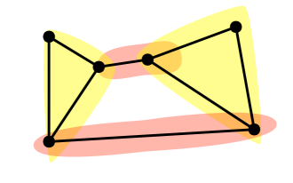
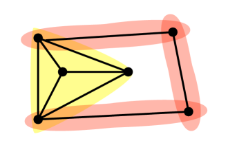
Figure 1: Examples of rigid components: (a) all the rigid components have size $2$ or $3$; (b) the indicated induced $K_{4}$ is rigid, but has one more edge than is required for minimal rigidity.

The combinatorial model for a bar-joint framework is a simple graph $G=(V,E)$ with $n$ vertices representing the joints, and $m$ edges representing the bars. A remarkable theorem of Maxwell-Laman [16, 18] says that rigidity for a generic framework (and almost all frameworks are generic) is determined by the underlying graph alone. The graph-theoretic condition characterizing minimal rigidity is a hereditary sparsity count; for minimal rigidity the graph $G$ should have $m=2n-3$ edges, and every subgraph induced by $n^{\prime}$ vertices in $G$ should have at most $2n^{\prime}-3$ edges. Therefore, by the Maxwell-Laman Theorem generic rigidity in the plane becomes a combinatorial concept, and from now on we will consider it as such. Full definitions are given in Section 2.

Contributions.

With this background, we can restate our main question as follows: What is the behavior of rigid components in a generic framework with its combinatorics given by an Erdős-Rényi random graph $G(n,p)$? Our main result is the following:

Theorem 1.1 ().

[Main Theorem] For any constant $c>0$ the following holds,

• If $c<c_{2}$, then, w.h.p., all rigid components in $G(n,c/n)$ span at most three vertices and

• If $c>c_{2}$, then, w.h.p., there is a unique giant rigid component in $G(n,c/n)$ spanning a $(1-o(1))$ fraction of the $(3+2)$-core.

The $(3+2)$-core of $G(n,c/n)$ is the maximal induced subgraph obtained by starting from the $3$-core and then inductively adding vertices with $2$ neighbors in the graph obtained so far (see Section 3 for the full definition). The constant $c_{2}\approx 3.588$ is the threshold for $2$-orientability discovered independently by Fernholz and Ramachandran [8] and Cain, Sanders, and Wormald [4]. A graph $G$ is $2$-orientable if all its edges can be oriented so that each vertex has out-degree at most two. There is a natural connection between the notions of $2$-orientability and minimal rigidity: $2$-orientable graphs can be characterized using a counting condition that closely resembles the counting condition of minimal rigidity (see Section 2). This connection explains intuitively why the threshold for the emergence of giant rigid component should be at least $c_{2}$. For example, if a giant rigid component emerges with $c<c_{2}$, then addition of another $o(n)$ random edges would create, with high probability, a “locally dense” induced subgraph with more than twice the number of edges than vertices. This prevents the graph from being $2$-orientable, contradicting the $2$-orientability threshold theorems of [8, 4].

We prove the bound on the size of the giant rigid component by showing this following result.

Theorem 1.2 ().

Let $c>c_{2}$ be a constant. Then, w.h.p., there is a subgraph of the $(3+2)$-core such that the edges of this subgraph can be oriented to give all but $O(\log^{3}n\sqrt{n})$ of the vertices in the $(3+2)$-core an out-degree of two.

The results of [8, 4] show that for $c>c_{2}$, with high probability $G(n,c/n)$ is not $2$-orientable, they don’t give quantitative bounds on the size of the set of vertices in $G(n,c/n)$ that can be guaranteed an out-degree $2$. Theorem 1.2, achieves this goal. Our proof for Theorem 1.2 is constructive and uses an extension of the $2$-orientability algorithm of Fernholz and Ramachandran [8]. Our analysis is quite different from [8] and is based on proving subcriticality of the various branching processes generated by our algorithm. We use differential equations to model the branching process, and show subcriticality by analyzing these differential equations.

Other Related Work.

Jackson et al. [12] studied the space of random $4$-regular graphs and showed that with high probability they are globally rigid (a stronger notion of rigidity [6]). In the $G(n,p)$ model they prove that when $p=n^{-1}(\log n+2\log\log n+\omega(1))$, then with high probability $G(n,p)$ is rigid, but they have no results for $G(n,p)$ when the expected number of edges is $O(n)$. In a recent result, Theran [27] showed using a simple counting argument that for a constant $c$ w.h.p. all rigid components in $G(n,c/n)$ are either tiny or giant. Since we use this result as a technical tool, it is introduced in more detail in Section 3.

Organization.

This paper is organized as follows. We introduce the required background in combinatorial rigidity in Section 2 (rigidity experts may skip this section), and the technical tools from random graphs we use to prove Theorem 1.1 in Section 3 (random graphs experts may skip this section). With the background in place, we prove some graph theoretic lemmas in Section 4. The proof that Theorem 1.2 implies Theorem 1.1 is in Section 5.

The remainder of the paper is devoted to the proof of Theorem 1.2. Section 6 introduces the facts about the random configuration model we need, and then we present our $2$-orientation algorithm in Section 7. Section 8 proves Theorem 1.2.

Notations.

Throughout this paper $G$ is a graph $(V,E)$ with $|V|=n$ and $|E|=m$. All our graphs are simple unless explicitly stated otherwise. Subgraphs are typically denoted by $G^{\prime}$ with $n^{\prime}$ vertices and $m^{\prime}$ edges. Whether a subgraph is edge-induced or vertex-induced is always made clear. A spanning subgraph is one that includes the entire vertex set $V$.

Erdős-Rényi random graphs on $n$ vertices with edge probability $p$ are denoted $G(n,p)$. Since we are interested in random graphs with constant average degree, we use the parameterization $G(n,c/n)$, where $c>0$ is a fixed constant.

Asymptotics.

We are concerned with the asymptotic behavior of $G(n,c/n)$ as $n\to\infty$. The constants implicit in the $O(\cdot)$, $\Omega(\cdot)$, $\Theta(\cdot)$; and the convergence implicit in $o(\cdot)$ are all taken to be uniform. A sequence of events $\mathcal{E}_{n}=(E_{n})_{n=1}^{\infty}$ holds with high probability (shortly w.h.p.) if $\Pr\left[E_{n}\right]=1-o(1)$.

2 Rigidity preliminaries

In this section, we introduce the notations of and a number of standard results on combinatorial rigidity that we use throughout. All of the (standard) combinatorial lemmas presented here can be established by the methods of (and are cited to) [17, 10], but we give some proofs for completeness and to introduce non-experts to style of combinatorial argument employed below.

Sparse and Spanning Graphs.

A graph $G$ with $n$ vertices and $m$ edges is $(k,\ell)$-sparse if, for all edge-induced subgraphs on $n^{\prime}$ vertices and $m^{\prime}$ edges, $m^{\prime}\leq kn^{\prime}-\ell$. If, in addition $m=kn-\ell$, $G$ is $(k,\ell)$-tight. If $G$ has a $(k,\ell)$-tight spanning subgraph it is $(k,\ell)$-spanning. When $k$ and $\ell$ are non-negative integer parameters with $\ell\in[0,2k)$ the $(k,\ell)$-sparse graphs form a matroidal family [17, Theorem 2] with rich structural properties, some of which we review below. In the interest of brevity, we introduce only the parts of the theory required.

In particular, throughout, we are interested in only two settings of the parameters $k$ and $\ell$: $k=2$ and $\ell=3$; and $k=2$ and $\ell=0$. For economy, we establish some standard terminology following [17]. A $(2,3)$-tight graph is defined to be a Laman graph; a $(2,3)$-sparse graph is Laman-sparse; a $(2,3)$-spanning graph is Laman-spanning.

The Maxwell-Laman Theorem and Combinatorial Rigidity.

The terminology of Laman graphs is motivated by the following remarkable theorem of Maxwell-Laman.

Proposition 2.1.

(Maxwell-Laman [18, 16]) A generic bar-joint framework in the plane is minimally rigid if and only if its graph is a Laman graph.

An immediate corollary is that a generic framework is rigid, but not necessarily minimally so, if and only if its graph is Laman-spanning. From now on, we will switch to the language of sparse graphs, since our setting is entirely combinatorial.

Rigid Blocks and Components.

Let $G$ be a graph. A rigid block in $G$ is defined to be a vertex-induced Laman-spanning subgraph. We note that if a block is not an induced Laman graph, then there may be many different choices of edge sets certifying that it is Laman spanning. A rigid component of $G$ is an inclusion-wise maximal block. As a reminder to the reader, although we have retained the standard terminology of “rigid” components, these definitions are graph theoretic.

A Laman-basis of a graph $G$ is a maximal subgraph of $G$ that is Laman-sparse. All of these are the same size by the matroidal property of Laman graphs [17, Theorem 2], and each rigid block in $G$ induces a Laman graph on its vertex set in any Laman basis of $G$. Thus, we are free to pass through to a Laman basis of $G$ or any of its rigid components without changing the rigidity behavior of $G$.

We now present some properties of rigid blocks and components that we use extensively.

Lemma 2.1 ([17, Theorem 5]).

Any graph $G$ decomposes uniquely into rigid components, with each edge in exactly one rigid component. These components intersect pairwise on at most one vertex, and they are independent of the choice of Laman basis for $G$

Proof.

Since a single edge forms a rigid block, each edge must be in a maximal rigid block, which is the definition of a components. By picking a Laman basis of $G$, we may assume, w.l.o.g., that $G$ is Laman-sparse. In that case, it is easy to check that two rigid blocks intersecting on at least two vertices form a larger rigid block. Since components are rigid blocks, we then conclude that components intersect on at most one vertex. The rest of the lemma then follows from edges having two endpoints. ∎

Lemma 2.2 ([17, Theorem 2]).

Adding an edge to a graph $G$ never decreases the size of any rigid component in $G$; i.e., rigidity is a monotone property of graphs.

Proof.

There are two cases: either the new edge has both endpoints in a rigid component of $G$ or it does not. In the first case, the component was already a Laman-spanning induced subgraph and remains that way. In the second case, Lemma 2.1 implies that the new edge is in exactly one component of the new graph; this may subsume other components of $G$ or be just the new edge. Either way, all of the components of $G$ remain rigid blocks in the new graph. ∎

The following lemma is quite well-known.

Lemma 2.3.

Let $G$ be a graph, and let $G_{1}=(V_{1},E_{1})$ and $G_{2}=(V_{2},E_{2})$ be rigid blocks in $G$ and suppose that either:

• $V_{1}\cap V_{2}=\emptyset$ and there are at least three edges with one endpoint in $V_{1}$ and the other in $V_{2}$, and these edges are incident on at least two vertices in $V_{1}$ and $V_{2}$

• $V_{1}\cap V_{2}\neq\emptyset$ (and so by Lemma 2.1 the intersection is a single vertex $v$) and there is one edge $ij$ with $i\in V_{1}$, $j\in V_{2}$ and $i$ and $j$ distinct from $v$

Then $V_{1}\cup V_{2}$ is a rigid block in $G$.

Proof.

There are two cases to check. In either case, by Lemma 2.1 it is no loss of generality to assume that $G_{1}$ and $G_{2}$ are Laman graphs on $n_{1}$ and $n_{2}$ vertices. The stated result follows from picking bases.

If $V_{1}$ and $V_{2}$ are disjoint, we further assume that there are exactly three edges going between them. Call this set $E_{3}$. Since the $E_{i}$ are disjoint by Lemma 2.1, we see that $V_{1}\cup V_{2}$ spans $2(n_{1}+n_{2})-3$ total edges. Taking an arbitrary subset $V^{\prime}\subset V_{1}\cup V_{2}$ of $n^{\prime}$ vertices, we see that it spans at most $|E_{1}\cap E(V^{\prime}\cap V_{1})|+|E_{2}\cap E(V^{\prime}\cap V_{2})|+3=2n^{\prime}-3$ edges, proving that $V_{1}\cup V_{2}$ spans an induced Laman graph.

The cases where $V_{1}$ and $V_{2}$ is similar, after accounting for a one-vertex overlap with inclusion-exclusion. ∎

Lemma 2.4 ([17, Corollary 6]).

If $G$ is a simple graph on $n$ vertices and has $m>2n-3$ edges, then $G$ spans a rigid block that is not Laman-sparse on at least four vertices. This block has minimum vertex degree at least $3$.

Proof.

Since $G$ has more than $2n-3$ edges, it is not Laman-sparse. Select an edge-wise minimal subgraph $G^{\prime}$ on $n^{\prime}$ vertices and $m^{\prime}$ edges that is not Laman-sparse, and, additionally, make $n^{\prime}$ minimum. By minimality of $m^{\prime}$, $m^{\prime}=2n^{\prime}-2$, and since $G$ is simple, $G^{\prime}$ is not a doubled edge, and thus has at least four vertices. Since dropping any edge from $G^{\prime}$ results in a subgraph on the same vertices with $2n^{\prime}-3$ edges that is Laman-sparse, $G^{\prime}$ is Laman-spanning, giving the desired rigid block. Finally, removing a degree one or two vertex from $G^{\prime}$ would result in a smaller subgraph that is not Laman-sparse, so minimality of $n^{\prime}$ implies that $G^{\prime}$ has minimum vertex degree $3$. ∎

Lemma 2.5 ([17, Lemma 4]).

If $G=(V,E)$ is Laman-spanning graph on $n$ vertices, then $G$ has minimum degree at least two.

Proof.

Pick a Laman basis $G^{\prime}$ of $G$. If $G^{\prime}$ has a degree one vertex $v$, then $V-v$ spans $2n-4>2(n-1)-3$ edges, contradicting the assumption that $G^{\prime}$ was a Laman graph. Thus no graph $G$ with a degree one vertex can have a spanning subgraph that is a Laman graph. ∎

Lemma 2.6 ([17, Lemma 17]).

If $G=(V,E)$ is a Laman-spanning graph on $n$ vertices, removing a degree two vertex results in a smaller Laman-spanning graph.

Proof.

Let $v$ be a degree two vertex in $G$. Pick a Laman basis $G^{\prime}$ of $G$. By Lemma 2.5, both edges incident on $v$ are in $G^{\prime}$. In $G^{\prime}$, $V-v$ spans $2n-3-2=2(n-1)-3$ edges, implying that $V-v$ induces a smaller Laman graph in $G^{\prime}$, from which it follows that $V-v$ is Laman-spanning. ∎

$2$-orientatbility and $(2,0)$-sparsity.

We now consider the structure properties of $(2,0)$-sparse graphs. The properties we review here can be obtained from [10]. A graph $G$ is defined to be $2$-orientable if its edges can be oriented such that each vertex has out-degree at most $2$. There is a close connection between $2$-orientability and $(2,0)$-sparsity expressed in the following lemma.

Lemma 2.7 ([10, Lemma 6] or [17, Theorem 8 and Lemma 10]).

A graph $G$ is $(2,0)$-tight if and only if it is a maximal $2$-orientable graph.

Proof sketch.

If $G=(V,E)$ is maximal and $2$-orientable, is has $n$ vertices and $2n$ edges. Counting edges by their tails in an out-degree at most two orientation, any subset of $n^{\prime}$ vertices is incident on, and therefore induces, at most $2n^{\prime}$ edges. On the other hand, the sparsity counts and Hall’s Matching Theorem implies that the bipartite graph with vertex classes indexed by $E$ and two copies of $V$ with edges between “edge vertices” and the copies of their endpoints has a perfect matching. The matching yields the desired orientation by orienting edges into the vertex they are matched to, as there are two copies of every vertex in the bipartite graph. ∎

As a corollary, we obtain,

Lemma 2.8 ([17, Theorem 8 and Lemma 10]).

A graph $G$ is $2$-orientable if and only if it is $(2,0)$-sparse.

Proof.

If $G$ is $2$-orientable, than any subset $V^{\prime}$ of $n^{\prime}$ vertices is incident on, and thus induces, at most $2n^{\prime}$ edges. On the other hand, if $G$ is $(2,0)$-sparse, extend it to being $(2,0)$-tight and then apply Lemma 2.7 to get the required orientation. ∎

Henneberg Moves and $2$-orientability.

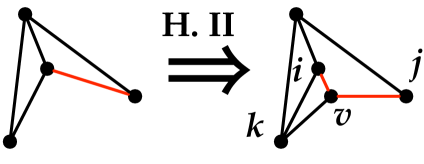
Figure 2: Examples of the Henneberg moves: (a) Henneberg I; (b) Henneberg II. In (b), the edge that is “split,” and the two new edges that replace it, are shown in red.

In our analysis of the $2$-orientation heuristic, we will make use of so-called Henneberg moves, which give inductive characterizations of all $(k,\ell)$-sparse graphs. Henneberg moves originate from [11] and are generalized to the entire family of $(k,\ell)$-sparse graphs in [17]. The moves are defined as follows:

Henneberg I:

Let $G$ be a graph on $n-1$ vertices. Add a new vertex $v$ to $G$ and two new edges to neighbors $i$ and $j$.

Henneberg II:

Let $G$ be a graph on $n-1$ vertices, and let $ij$ be an edge in $G$. Add a new vertex $v$ to $G$, select a neighbor $k$, remove the edge $ij$, and add edges between $v$ and $i$, $j$, and $k$.

Figure 2 shows examples of the two moves. Since we are concerned with $(2,0)$-sparsity, while $v$ must be new, the neighbors $i$, $j$, and $k$ may be the same as each other or $v$. When this happens we get self-loops or multiple copies of the same edge (i.e., a multigraph). The fact we need later is,

Lemma 2.9 ([17, Lemma 10 and Lemma 17] or [8]).

The Henneberg moves preserve $2$-orientability.

We give a proof for completeness, since we will use the proof idea later.

Proof.

Assume $G$ is $2$-orientable. For the Henneberg I move, orient the two new edges out of the new vertex $v$. For the Henneberg II move, suppose that $ij$ is oriented $i\to j$ in $G$. Orient the new edges $i\to v$, $v\to j$, $v\to k$. ∎

We remark that although the development here follows along the lines of the rigidity-inspired [17], this idea was developed (to our knowledge) independently by Fernholz and Ramachandran [8].

Almost Spanning Subgraphs.

We introduce a final piece of notation, which is the concept of an almost spanning graph. A graph $G$ on $n$ vertices is defined to be almost $(2,0)$-spanning if it contains a $(2,0)$-spanning subgraph on $n-o(n)$ vertices.

The Explosive Growth of Rigid Components.

Figure 3: A family of graphs in which adding any edge rigidifies the entire graph.

We conclude this section with an example that shows how the behavior of rigid components can be very different than that of connectivity. Unlike connectivity, the size of the largest rigid component in a graph may increase from $O(1)$ to $\Omega(n)$ after adding only one edge. A dramatic family of examples is due to Ileana Streinu [25]. We begin with the graph obtained by dropping an edge from $K_{3,3}$; this graph has $2\cdot 6-4=8$ edges, and its rigid components are simply the edges. We then repeatedly apply the Henneberg II move, avoiding triangles whenever possible. As we increase the number of vertices $n$, for even $n$, we obtain graphs with $2n-4$ edges and no rigid components spanning more than two vertices (see Figure 3(c)); but adding any edge to these graphs results in a Laman-spanning graph.

This example can be interpreted as saying that rigidity is an inherently non-local phenomenon.

3 Random graphs preliminaries

Let $G(n,p)$ be a random graph on $n$ vertices where each edge appears independently of all others with probability $p$. In this paper, we are interested in sparse random graphs, which are generated by $p=c/n$ for some constant $c$. This section introduces the results from random graphs that we need as technical tools, along with our Theorem 1.2 to prove the main Theorem 1.1.

Size of the $3$-core.

The $k$-core of a graph is defined as the maximal induced subgraph of minimum degree at least $k$. The $k$-core thresholds for random graphs have been studied in [23, 7, 19, 15]. For $\mu>0$, let $Po(\mu)$ denote a Poisson random variable with mean $\mu$. Let us denote the Poisson probabilities by $\pi_{j}(\mu)=\Pr[Po(\mu)=j]$. Let $\psi_{j}(\mu)=\Pr[Po(\mu)\geq j]$. Also, let $\lambda_{k}=\min_{\mu>0}\mu/\psi_{k-1}(\mu).$ For $\lambda>\lambda_{k}$, let $\mu_{k}(\lambda)>0$ denote the largest solution to $\mu/\psi_{k-1}(\mu)=\lambda$. In [23], Pittel, Spencer and Wormald discovered that for $k\geq 3$, $\lambda=\lambda_{k}$ is the threshold for the appearance of a nonempty $k$-core in the random graph $G(n,\lambda/n)$.

Proposition 3.1 (Pittel, Spencer, and Wormald [23]).

Consider the random graph $G(n,\lambda/n)$, where $\lambda>0$ is fixed. Let $k\geq 2$ be fixed. If $\lambda<\lambda_{k}$, then w.h.p. the $k$-core is empty in $G(n,\lambda/n)$. If $\lambda>\lambda_{k}$, then w.h.p. there exists a $k$-core in $G(n,\lambda/n)$ whose size is about $\psi_{k}(\mu_{k}(\lambda))n$.

We will use the $k=3$ instance of Proposition 3.1. Substituting $k=3$ in the above equation gives $\lambda_{3}\approx 3.351$, and the size of the 3-core at $\lambda=\lambda_{3}$ is about $0.27n$.

The $(3+2)$-core.

Extending the $3$-core, we define the $3+2$-core of a graph as the maximal subgraph that can be constructed starting from the $3$-core and inductively adding vertices with at least two neighbors in the subgraph built so far.

From the definition, it is easy to see that the $(3+2)$-core emerges when the $3$-core does, and, since it contains the $3$-core, it it, w.h.p., empty or giant in a $G(n,p)$. A branching process heuristic indicates that, after it emerges, the fraction of the vertices in the $(3+2)$-core is the root $q$ of the equation $q=1-\mathrm{e}^{-qc}(1+qc)$ (where $\mathrm{e}^{-qc}(1+qc)$ comes from $\Pr[Po(qc)<2]$). However, we do not know how to make the argument rigorous, and so we leave it as a conjecture. At $c=3.588$ the conjectured number of vertices in the $(3+2)$-core is about $0.749n$.

The $2$-orientability Threshold.

Define the constant $c_{2}$ to be the supremum of $c$ such that the $3$-core of $G(n,c/n)$ has average degree at most $4$.

Fernholz and Ramachandran and Cain, Sanders, and Wormald independently proved that $c_{2}$ is the threshold for $2$-orientability of $G(n,c/n)$.

Proposition 3.2 ([8, 4]).

With high probability, for any fixed constant $c>0$:

• If $c<c_{2}$, $G(n,c/n)$ is $2$-orientable.

• If $c>c_{2}$, $G(n,c/n)$ is not $2$-orientable.

Rigid Components are Small or Giant.

An edge counting argument ruling out small dense subgraphs in $G(n,c/n)$ shows the following fact about rigid components in random graphs.

Proposition 3.3 (Theran [27]).

Let $c>0$ be a constant. Then, w.h.p., all rigid components in a random graph $G(n,c/n)$ have size $1$, $2$, $3$, or $\Omega(n)$.

4 Graph-theoretic lemmas

This short section gives the combinatorial lemmas we need to derive Theorem 1.1 from Theorem 1.2. The first is a simple observation relating adding edges to the span of a rigid component and $2$-orientability.

Lemma 4.1.

Let $G=(V,E)$ be a graph and let $G^{\prime}=(V^{\prime},E^{\prime})$ be a rigid component of $G$. Then after adding any $4$ edges to the span of $V^{\prime}$, the resulting graph is not $2$-orientable.

Proof.

Let $V^{\prime}$ have $n^{\prime}$ vertices. Since $G^{\prime}$ is a rigid component, it has a Laman basis by definition and thus spans at least $2n^{\prime}-3$ edges. After the addition of $4$ edges to the span of $V^{\prime}$, it spans at least $2n^{\prime}+1$ edges, blocking $2$-orientability by Lemma 2.8. ∎

Another simple property we will need is that if $G$ is not Laman-sparse it spans a rigid component with non-empty $(3+2)$-core.

Lemma 4.2.

Let $G$ be a simple graph that is not Laman-sparse. Then $G$ spans a rigid component on at least four vertices that is contained in the $(3+2)$-core.

Proof.

Since $G$ is simple and fails to be Laman sparse, the hypothesis of Lemma 2.4 is met, so there is a rigid block in $G$ with a non-empty $3$-core. The component containing this block has minimum degree two by Lemma 2.5, and peeling off degree two vertices will never result in a degree one vertex by Lemma 2.6, so it is in the $(3+2)$-core. ∎

We conclude with the main graph-theoretic lemma we need.

Lemma 4.3.

Let $G=(V,E)$ be a simple graph that:

• coincides with its $(3+2)$-core;

• spans a rigid component $G^{\prime}=(V^{\prime},E^{\prime})$ on $n^{\prime}\geq 4$ vertices;

• and the set of $n^{\prime\prime}$ vertices $V^{\prime\prime}=V\setminus V^{\prime}$ is incident on at least $2n^{\prime\prime}$ edges.

Then at least one of the following is true

• $G$ is Laman-spanning

• $G$ spans a rigid component other than $G^{\prime}$ on at least $4$ vertices

Proof.

Pick a Laman basis for $G^{\prime}$ and discard the rest of the edges spanned by $V^{\prime}$. Call the remaining graph $H$. Observe that $G$ and $H$ have the same rigid components. By hypothesis, $H$ now has at least $2n^{\prime}-3+2n^{\prime\prime}=2n-3$ edges. If $H$ is Laman-spanning we are done, so we suppose the contrary and show that this assumption implies the second conclusion.

Because $H$ is not Laman-spanning and has $2n-3$ edges, it must not be Laman-sparse. By Lemma 2.4, $H$ spans a rigid block that is not Laman-sparse, and this block must be contained in some rigid component $H^{\prime}$ of $H$. Finally, since $V^{\prime}$ induces a Laman-sparse rigid component of $H$ and $H^{\prime}$ is a rigid component that isn’t Laman-sparse, $H^{\prime}$ and $G^{\prime}$ are different rigid components of $H$ and thus $G$. ∎

5 Proof of the Main Theorem 1.1

In this section, we prove our main theorem:

Roadmap.

The structure of this section is as follows. We start by establishing that the constant $c_{2}$ is the sharp threshold for giant rigid components to emerge. This is done in two steps:

• That there is a giant rigid component, w.h.p., when $c>c_{2}$ is the easier direction, coming from counting the number of edges in the $3$-core using Proposition 3.2. (Lemma 5.2)

• The more difficult direction is that when $c<c_{2}$ all components are w.h.p. size two or three is proved using the following idea: if there is a giant rigid component, adding $\Theta(1)$ more random edges will block $2$-orientability, contradicting Proposition 3.2. (Lemma 5.1)

The idea of the proof of the size of the giant rigid component is to apply the main combinatorial Lemma 4.3 to the $(3+2)$-core of $G(n,c/n)$ after adding a small number of uniform edges. This is possible as a consequence of the more technical Theorem 1.2. Since only the first conclusion of Lemma 4.3 is compatible with Proposition 3.3, w.h.p., the presence of a large enough giant rigid component follows. Before we can do that we establish two important structural properties:

• There is a unique giant rigid component, w.h.p., (Lemma 5.3)

• It is contained in the $(3+2)$-core (Lemma 5.4)

With these results, Lemma 5.6 formalizes the plan described above, and Theorem 1.1 follows.

Sharp Threshold.

We first establish that $c_{2}$ is the sharp threshold for emergence of giant rigid components. This is done in the next two lemmas, starting with the more difficult direction.

Lemma 5.1.

Let $c<c_{2}$. Then w.h.p, $G(n,c/n)$ has only rigid components of size at most three.

Proof.

Proposition 3.3 implies that all rigid components in $G(n,c/n)$ have size at most three or are giant. We will show that, w.h.p., there are no giant rigid components. Let $\Gamma$ be the event that $G$ spans a rigid component $G^{\prime}=(V^{\prime},E^{\prime})$ on $n^{\prime}>3$ vertices and $m^{\prime}$ edges.

Define the graph $H$ to be the one obtained by adding edges sampled with probability $1/n^{2}$, independently, from the complement of $G$ in $K_{n}$. Since $H$ is a random graph with edge probability $(c+1/n)/n$, by Proposition 3.2 $H$ is, w.h.p., $2$-orientable so:

$$\begin{split}\Pr\left[\text{$H$ is not $2$-orientable}|\Gamma\right]\Pr\left[\Gamma\right]+\\ \Pr\left[\text{$H$ is not $2$-orientable}|\bar{\Gamma}\right]\Pr\left[\bar{\Gamma}\right]=o(1)\end{split}$$

We will show that $\Pr\left[\text{$H$ is not $(2,0)$-sparse}|\Gamma\right]$ is uniformly bounded away from zero, which then forces the probability of a rigid component on more than three vertices to be $o(1)$.

If $\Gamma$ holds, Proposition 3.3 implies that, $n^{\prime}=\Omega(n)$, w.h.p. It follows that, conditioned on $\Gamma$, each of the added edges is in the span of $V^{\prime}$ with probability $(1-o(1))\frac{1}{n^{2}}\Omega(n^{2})=\Theta(1)$, so the probability that at least four of them end up in the span of $V^{\prime}$ is $\Theta(1)$ as well. This shows that with probability $\Theta(1)$, the combinatorial lemma Lemma 4.1 applies and so

$$\Pr\left[\text{$H$ is not $2$-orientable}|\Gamma\right]=\Theta(1).$$

∎

Lemma 5.2.

Let $c>c_{2}$. Then w.h.p., $G(n,c/n)$ has at least one giant rigid component.

Proof.

By Lemma 2.4, any simple graph with $n$ vertices and at least $2n-2$ edges spans a rigid block on at least $4$ vertices. Proposition 3.2 implies that for $c>c_{2}$, the $3$-core of $G(n,c/n)$ induces such a graph w.h.p. Finally Proposition 3.3 implies that there is a giant rigid component w.h.p. ∎

Uniqueness of the Giant Rigid Component.

Before we determine the size, we show that w.h.p. there is only one giant rigid component and that it is contained in the $(3+2)$-core.

Lemma 5.3.

Let $c>c_{2}$. Then w.h.p., there is a unique giant rigid component in $G(n,c/n)$.

Proof.

By Lemma 5.2, when $c>c_{2}$ w.h.p. there is at least one giant rigid component in $G(n,c/n)$. To show the giant rigid component is unique, we consider $G(n,c/n)$ as being generated by the following random graph process: first select a linear ordering of the $\binom{n}{2}$ edges of $K_{n}$ uniformly at random and take the first $m$ edges from this ordering, where $m$ has binomial distribution with parameters $\binom{n}{2}$ and $c/n$.

Consider the sequence of graphs $G_{1},G_{2},\ldots,G_{\binom{n}{2}}$ defined by adding the edges one at a time according to the selected ordering. Define $t\in[1,\binom{n}{2}]$ to be critical if $G_{t}$ has one more rigid component spanning more than three vertices than $G_{t-1}$ and bad if $G_{t}$ has more than one such rigid component.

By Proposition 3.3, w.h.p., all rigid components on more than three vertices that appear during the process have size $\Omega(n)$. Thus, w.h.p., at most $O(1)$ $t$ are critical.

To bound the number of bad $t$ we note that if $G^{\prime}=(V^{\prime},E^{\prime})$ and $G^{\prime\prime}=(V^{\prime\prime},E^{\prime\prime})$ are distinct giant rigid components, then the probability that a random edge has one endpoint in $V_{1}\setminus V_{2}$ and the other in $V_{2}\setminus V_{1}$ is $\Theta(1)$, and the probability that two of the added edges are incident on the same vertex is $O(1/n)$. So after the addition of $O(\log n)$ random edges, at least three of them have this property, w.h.p. Lemma 2.3 then implies that, w.h.p., $G^{\prime}$ and $G^{\prime\prime}$ persist as giant rigid components for at most $O(\log n)$ steps in the process. Since there are at most $O(1)$ such pairs, the total number of bad or critical $t$ is $O(\log n)$, w.h.p.

The probability that $m=t$ is $O(1/\sqrt{n})$, by standard properties of the binomial distribution. A union bound shows that the probability $m$ is bad is $O(\log n/\sqrt{n})$, so the probability there is only one rigid component on more than three vertices and that it is giant is $1-o(1)$ as desired. ∎

We need two more structural lemmas about the relationship between the giant rigid component and the $(3+2)$-core.

Lemma 5.4.

Let $c>c_{2}$. Then, the unique giant rigid component that exists w.h.p. by Lemma 5.3 is contained in the $(3+2)$-core of $G(n,c/n)$. Moreover, the giant rigid component contains a (smaller) unique giant rigid block that lies entirely in the $3$-core.

Proof.

By Lemma 5.3, w.h.p., $G(n,c/n)$ has exactly one rigid component of size at least $4$, and it spans at least twice as many edges as vertices. Thus Lemma 4.2 applies to the rigid component, w.h.p., so it is in the $(3+2)$-core. Because the $3$-core itself has average degree at least $4$, the second part of the lemma follows from the same argument. ∎

Lemma 5.5.

Let $c>c_{2}$ and suppose that the giant rigid block in the $3$-core implied by Lemma 5.4 spans all but $o(n)$ of the vertices in the $3$-core. Then, w.h.p., the giant rigid component spans all but $o(n)$ vertices in the $(3+2)$-core.

Proof.

Since $c>c_{2}$, both the $3$-core and the $(3+2)$-core span $\Omega(n)$ vertices, w.h.p. If the $(3+2)$-core has $o(n)$ more vertices than the $3$-core, then we are already done. Thus for the rest of the proof, we assume that the $(3+2)$-core spans $\Omega(n)$ more vertices than the $3$-core.

Let $G$ denote $G(n,c/n)$, let $G_{0}=(V_{0},E_{0})$ denote the $3$-core, let $G_{1}=(V_{1},E_{1})$ be the $(3+2)$-core, and let $G^{\prime}=(V^{\prime},E^{\prime})$ be the giant rigid block in the $3$-core. We now observe that each $v\in V_{1}-V_{0}$ sits at the “top” of a binary tree with its “leaves” in $V_{0}$. A branching process argument shows that each of these has height at most $\log\log n$, w.h.p. On the other hand, a vertex $v\in V_{0}$ is in the giant rigid component when all of these $O(\log n)$ “leaves” lie in $V^{\prime}$. Since $V_{0}-V^{\prime}$ has $o(n)$ vertices, this happens with probability $1-o(1)$. ∎

Size of the giant rigid component.

We are now ready to bound the size of the giant rigid component when it emerges. Here is the main lemma.

Lemma 5.6.

Let $c>c_{2}$. Then, w.h.p., the unique giant rigid component implied by Lemma 5.3 spans a $(1-o(1))$-fraction of the vertices in the $(3+2)$-core.

Proof.

Let $G=G(n,c/n)$, let $G_{0}=(V_{0},E_{0})$ be the $3$-core of $G$, and let $G^{\prime}=(V^{\prime},E^{\prime})$ be a giant rigid block of $G_{0}$ implied, w.h.p. by Lemma 5.4. Let $n_{0}$ be the size of $V_{0}$ and $n^{\prime}$ the size of $V^{\prime}$. With high probability, $n_{0}$ and $n^{\prime}$ are $\Omega(n)$.

By Theorem 1.2 (and this is the hard technical step), $V^{\prime\prime}=V_{0}\setminus V^{\prime}$ is incident on $2(n_{0}-n^{\prime})-O(\log^{3}n\,\sqrt{n})$ edges in $G_{0}$.

Define $H$ to be the graph obtained by adding each edge of $K_{n}\setminus G$ to $G$ with probability such that $H$ and $G(n,(c+1/n^{5/4})/n)$ are asymptotically equivalent.

Let $\gamma>0$ be a fixed constant and define $\Gamma$ to be the event that $n_{0}-n^{\prime}\geq\gamma n_{0}$; i.e., the giant rigid component spans at most a $(1-\gamma)$-fraction of the $(3+2)$-core in $G$. Conditioned on $\Gamma$, the expected number of edges added between $V^{\prime}$ and $V^{\prime\prime}$ is $\Theta(n^{3/4})$, so w.h.p., Lemma 4.3 applies to $V_{0}$ in $H$. Recall that Lemma 4.3 has two conclusions:

• $V_{0}$ induces a Laman-spanning subgraph

• $V_{0}$ spans multiple components spanning at least four vertices in $H$

The second case happens with probability $o(1)$ by Proposition 3.3, so w.h.p., $V_{0}$ is Laman-spanning in $H$.

To complete the proof, we note that by [23] adding $o(n)$ edges causes the $3$-core to grow by $o(n)$ vertices, w.h.p. Thus the $3$-core of $G$ spans all but $o(n)$ vertices in the $3$-core of $H$. Now Lemma 5.5 applies to $H$, showing that, w.h.p., all but $o(n)$ vertices in the $(3+2)$-core lie in the giant rigid component. ∎

Proof of Theorem 1.1.

The theorem follows from Lemma 5.1, Lemma 5.2, and Lemma 5.6. ∎

6 Configurations and the algorithmic approach

We now develop the setting used in the proof of Theorem 1.2, which is based on our analysis of a $2$-orientation heuristic for random graphs, which is introduced in the next section. The heuristic operates in the random configuration model (introduced in [1, 2]), which we briefly introduce here.

Random Configurations.

A random configuration is a model for random graphs with a pre-specified degree sequence; the given data is a vertex set $V$ and a list of degrees for each vertex such that the sum of the degrees is even. Define $deg(v)$ to denote the degree of a vertex $v\in V$.

A random configuration is formed from a set $\mathcal{A}$ consisting of $deg(v)$ copies of each vertex $v\in V$, defined to be the set of (vertex) copies of $V$. Let $\mathcal{M}$ denote a uniformly random perfect matching in $\mathcal{A}$. The multigraph $G_{\mathcal{A}}=(V,E)$ defined by $\mathcal{A}$ and $\mathcal{M}$ has $V$ as its vertex set and and edge $vw$ for each copy of a vertex $v$ matched to a copy of a vertex $w$.

The two key facts about random configurations that we use here are:

• Any property that is holds w.h.p. in $G_{\mathcal{A}}$ holds w.h.p. when conditioned on $G_{\mathcal{A}}$ being simple [20, 21].

• Any property that holds w.h.p. for $G_{\mathcal{A}}$ in a random configuration with asymptotically Poisson degrees holds w.h.p. in the sparse $G(n,c/n)$ model [3].

Since we are only interested in proving results on $G(n,c/n)$, from now all random configurations discussed have asymptotically Poisson degree sequences.

The Algorithmic Method.

Our proof of Theorem 1.2 relies on the following observation: a property that holds w.h.p. for any algorithm that generates a uniform matching $\mathcal{M}$ holds w.h.p. for a random configuration. The following two moves were defined by Fernholz and Ramachandran [8].

FR I

Let $\mathcal{A}$ be a set of vertex copies. Select (arbitrarily) any copy $a_{0}$ and match it to a copy $a_{1}$, selected uniformly at random. The matching $\mathcal{M}$ is given by the matched pair $\{a_{0},a_{1}\}$ and a uniform matching on $\mathcal{A}\setminus\{a_{0},a_{1}\}$.

FR II

Select two copies $a_{0}$ and $a_{1}$. Let $\mathcal{M}^{\prime}$ be a uniform matching on $\mathcal{A}\setminus\{a_{0},a_{1}\}$. Produce the matching $\mathcal{M}$ as follows:

• with probability $1/(|\mathcal{A}|-1)$ add the matched pair $\{a_{0},a_{1}\}$ to $\mathcal{M}^{\prime}$

• otherwise, select a matched pair $\{b_{0},b_{1}\}$ uniformly at random and replace it in $\mathcal{M}^{\prime}$ with the pairs $\{a_{0},b_{0}\}$, $\{a_{1},b_{1}\}$.

These two moves generate uniform matchings.

Lemma 6.1 ([8, Lemma 3.1]).

Matchings generated by recursive application of the moves FR I and FR II generate uniform random matchings on the set of vertex copies $\mathcal{A}$.

We will only use the move FRII in the special situation in which $a_{0}$ and $a_{1}$ are copies of the same vertex. With this specialization, in terms of the graph $G_{\mathcal{A}}$, the two moves correspond to:

FR I

Reveal an edge of $G_{\mathcal{A}}$ incident on the vertex $v$ that $a_{0}$ is a copy of.

FR II

Pick two copies $a_{0}$ and $a_{1}$ of a vertex $v$. Generate $G_{\mathcal{A}-\{a_{0},a_{1}\}}$ and then complete generating $G_{\mathcal{A}}$ by either adding a self-loop to $v$ or splitting the edge $ij$ corresponding to $\{b_{0},b_{1}\}$ by replacing it with edges $iv$ and $vj$, with probabilities as described above.

7 The $2$-orientation algorithm

We are now ready to describe our $2$-orientation algorithm. It generates the random multigraph $G_{\mathcal{A}}$ using the moves FR I and FR II in a particular order and orients the edges of $G_{\mathcal{A}}$ as they are generated.

Since Theorem 1.2 is only interested in the $(3+2)$-core, we assume that our algorithm only runs on the $(3+2)$-core of $G_{\mathcal{A}}$. Since we can always orient degree two vertices so that both incident edges point out, the only difficult part of the analysis is the behavior of our algorithm on the $3$-core of $G_{\mathcal{A}}$. We denote the set of copies corresponding to the $3$-core by $\mathcal{A}_{s}$ and the corresponding multigraph by $G_{\mathcal{A}_{s}}$. Define the number of copies of a vertex $v$ in $\mathcal{A}_{s}$ by $deg_{\mathcal{A}_{s}}(v)$.

The $2$-orientation Algorithm.

We now define our orientation algorithm in terms of the FR moves.

$2$-orienting the $3$-core Until $\mathcal{A}_{s}$ is empty, select a minimum degree vertex $v$ in $\mathcal{A}_{s}$, and let $d=deg_{\mathcal{A}_{s}}(v)$. 1. If $d\leq 2$, execute the FR I move, selecting a copy of $v$ deterministically. Orient the resulting edge or self-loop away from $v$. If $v$ still has any copies left, call this algorithm recursively, choosing $v$ as the minimum degree vertex. 2. If $d=3$, execute the FR II move, selecting two copies of $v$, and then recursively call this algorithm, starting the recursive call on $v$ using case $1$. If the FR II move generated a self-loop, orient it arbitrarily. If the FR II move split an oriented edge $i\to j$, orient the new edges $i\to v$ and $v\to j$. 3. If $d\geq 4$, perform FR I move on $v$, leaving the resulting edge unoriented. Then recursively call this algorithm, choosing $v$ as a minimum degree vertex.

We define a vertex $v$ to be processed if it is selected deterministically at any time. A vertex is defined to be tight if the algorithm orients exactly two edges out of it and loose otherwise. For convenience, when a vertex runs out of copies, we simply remove it from $\mathcal{A}_{s}$; thus when we speak of the number of remaining vertices, we mean the number of vertices with any copies left on them.

Correctness and Structural Properties.

We now check that the $2$-orientation algorithm is well-defined.

Lemma 7.1.

The $2$-orientation algorithm generates a uniform matching.

Proof.

This follows from the fact that it is based on the FR moves and Lemma 6.1. The only other thing to check is that if $v$ is being processed and the algorithm is called on $v$ again that $v$ is still a minimum degree vertex in $\mathcal{A}_{s}$. This is true, since $v$ started as minimum-degree and the FR moves decrease its degree at least as much as any other vertex. ∎

The following structural property allows us to focus only on the evolution of the degree sequence.

Lemma 7.2.

A loose vertex is $v$ generated only in one of three ways:

• $v$ is never processed, because it runs out of copies before it is selected

• $v$ has degree one in $\mathcal{A}_{s}$ when it is processed

• $v$ has degree two in $\mathcal{A}_{s}$ when it is processed, and a self-loop is revealed

Proof.

The proof is a case analysis.

• In step 1, if a self-loop is not generated, this is equivalent to the Henneberg I move, so by Lemma 2.9 $v$ ends up being tight.

• Step 2 always corresponds to a Henneberg II move or creates a self-loop, and so by Lemma 2.9 $v$ ends up being tight either way, and the out-degree of no other vertex changes.

• Step 3 cannot leave $v$ with fewer than two copies.

• The other cases are the ones in the statement of the lemma, completing the proof.

∎

Because of the algorithm’s recursive nature, we can, at any time, suspend the algorithm and just generate a uniform matching on the remaining configuration. In the next section, we will use this observation to split the analysis into two parts.

Lemma 7.3.

Let $\mathcal{A}_{s}|_{t}$ denote the remaining configuration at time $t$. Suppose that, w.h.p., a random configuration $G^{*}$ on $\mathcal{A}_{s}|_{t}$ is $(2,0)$-spanning. Then, w.h.p., there is an orientation of $G_{\mathcal{A}_{s}}$ in which all the vertices of $\mathcal{A}_{s}|_{t}$ are tight, and the out-degrees of vertices in $\mathcal{A}_{s}\setminus\mathcal{A}_{s}|_{t}$ are the same as in the full algorithm.

Proof.

Since $G^{*}$ comes from a uniform matching on the remaining copies, and the FR II move only requires this as input, the cut-off version of the $2$-orientation algorithm generates a uniform matching. Thus, w.h.p., results for it hold for $G_{\mathcal{A}_{s}}$.

By hypothesis, w.h.p., we can orient $G^{*}$ such that each vertex has out-degree at least two: $G^{*}$ has a subgraph that is $(2,0)$-spanning and orient the remaining edges arbitrarily, so all the vertices of $G^{*}$ are tight, w.h.p. Moreover, since before $G^{*}$ is generated, the cut-off algorithm acts the same way as the full algorithm, which implies that how we orient the edges of $G^{*}$ does not change the out-degrees in $\mathcal{A}_{s}\setminus\mathcal{A}_{s}|_{t}$.

So the final thing to check is that the FR I and FR II moves don’t change the out-degrees in $G^{*}$ after the recursive calls return to them.

• For FR I, no edges induced by $G^{*}$ are involved, so the statement is trivial.

• For FR II, either a self-loop is generated, in which case the proof is the same as for FR I; or an edge is split, in which case the construction used to prove Lemma 2.9 shows that the out-degree of vertices in $G^{*}$ remains unchanged.

This completes the proof. ∎

The Simplified Algorithm.

In light of Lemma 7.2, we can simplify the analysis by simply tracking how the degree sequence evolves as we remove copies from $\mathcal{A}_{s}$. Since loose vertices are generated only when a vertex runs out of copies before the algorithm had a chance to orient two edges out of them, we can ignore the edges and just remove copies as follows.

Simplified $2$-orientation algorithm Repeatedly execute the following on a vertex $v$ of minimum degree in $\mathcal{A}_{s}$, until $\mathcal{A}_{s}$ is empty 1. If $deg_{\mathcal{A}_{s}}(v)\leq 2$, repeat the loop until all copies of $v$ are removed
      a. remove a copy of $v$ from $\mathcal{A}_{s}$.
      b. remove a copy chosen uniformly at random from $\mathcal{A}_{s}$. 2. If $deg_{\mathcal{A}_{s}}(v)=3$, first remove the $2$ copies of $v$ from $\mathcal{A}_{s}$; then execute step 1. 3. If $deg_{\mathcal{A}_{s}}(v)\geq 4$, repeat the following loop $deg_{\mathcal{A}_{s}}(v)-3$ times and then execute step 2
      a. remove a copy of $v$ from $\mathcal{A}_{s}$.
      b. remove a copy chosen uniformly at random           from $\mathcal{A}_{s}$.

As a corollary to Lemma 7.2 we have,

Lemma 7.4.

The number of loose vertices generated by the simplified algorithm is exactly the number of vertices that run out of copies as in L$1$–L$3$ in Lemma 7.2

Proof.

The number of remaining copies of each vertex in $\mathcal{A}_{s}$ evolves as in the full algorithm. ∎

8 Proof of Theorem 1.2

In this section we prove,

Roadmap.

The proof is in two stages: before the minimum numbers of copies on any vertex remaining reaches four and after. The overall structure of the argument is as follows:

• At the start, the minimum number of copies on any vertex in $\mathcal{A}_{s}$ is three. We run the simplified algorithm until the minimum degree in $\mathcal{A}_{s}$ rises to four, or the number of vertices remaining reaches $\sqrt{n}$.

• Since we only run the simplified algorithm when there are are $\Omega(\sqrt{n})$ copies remaining, we can give bounds on the number of loose vertices generated by analyzing it as a series of branching processes.

• Once the minimum degree in $\mathcal{A}_{s}$ has reached four, we can use the combinatorial Lemma 4.3 along with the counting argument Proposition 3.3 to show that, w.h.p., a random configuration on what remains is $(2,0)$-spanning. If it never does, we just declare the last $\sqrt{n}$ vertices to be loose, so either way we get the desired bound.

We define the first stage, when we run the simplified algorithm, to be phase $3$; the second stage is phase $4$. The main obstacle is that during phase 3, there may be many degree two vertices, which increases the probability of generating loose vertices. Let us briefly sketch our approach.

At the start of phase 3, every vertex has degree at least three (and $\Omega(n)$ have degree three, w.h.p.). The algorithm will:

• Pick a degree three vertex, remove all of its copies and a random copy.

• Removing the random copy may create a degree two vertex, which is then removed, along with two random copies.

• These random copies may create more degree two vertices or even a loose vertex.

We call the cascade described above a round of the algorithm. We model each round as a branching process, which we analyze with a system of differential equations (this step occupies most of the section). The key fact is that, with high probability, all rounds process $O(\log n)$ vertices, which is enough to bound the number of loose vertices using arguments similar to those from the high-degree phase analysis.

Phase 3: The Main Lemma.

We start with the analysis of phase $3$. In phase $3$, all iterations of the algorithm take step 1 or 2. We define a round of the algorithm in phase $3$ to start with a step 2 iteration and contain all the step 1 iterations before the next step 2. The critical lemmas are.

Lemma 8.1.

With probability at least $1-1/n$, all rounds during phase $3$ process $O(\log n)$ vertices.

We defer the proofs for now, and instead show how they yield a bound on the number of loose vertices.

Lemma 8.2.

With high probability, the expected number of loose vertices generated in a phase $3$ round is $O(\log^{2}n/\sqrt{n})$.

Proof.

All vertices start the round with at least three copies on them, so Lemma 7.2 implies that a loose vertex is either

• hit at least twice at random (L1 and L2)

• reaches degree two and then gets a self-loop (L3)

Both of these events happen with probability $O(1/\sqrt{n})$, since we are only running the algorithm with this many vertices left, and the probability any specific vertex is hit is $O(1/k)$, where $k$ is the number of remaining copies, and w.h.p. this is $\Omega(n)$ during any phase 3 round.

Since the round lasts $O(\log n)$ iterations, w.h.p., the probability any vertex becomes loose is at most $O(\log n/\sqrt{n})$. Because any loose vertex generated in a round must be processed in that round, the expected number of loose vertices generated is $O(\log n)O(\log n/\sqrt{n})=O(\log^{2}n/\sqrt{n})$. ∎

Lemma 8.3.

With high probability, the number of loose vertices generated during phase $3$ is $O(\log^{3}n\sqrt{n})$.

Proof.

Let $\Gamma$ be the event that all rounds process $O(\log n)$ vertices. The main Lemma 8.1 implies that $\Gamma$ fails to hold with probability $1/n$, so we are done if the lemma holds when conditioning on $\Gamma$.

Assuming, $\Gamma$, Lemma 8.2 applies to $O(n)$ rounds. From Lemma 8.2, we see that, w.h.p., the expected number of loose vertices generated in phase $3$ is $O(n)O(\log^{2}/\sqrt{n})=O(\log^{2}n\sqrt{n})$. It then follows from Markov’s inequality that the probability of $\Omega(\log^{3}n\sqrt{n})$ loose vertices generated in phase $3$ is at most $1/\log n=o(1)$.

If phase $3$ runs until it hits its cutoff point, then there are an additional $O(\sqrt{n})$ loose vertices, but this preserves the desired bound. ∎

Phase 4.

At the start of phase $4$, we stop the simplified algorithm, since we can prove the following lemma more directly.

Lemma 8.4.

With high probability, at the start of phase $4$, a uniform simple graph generated from $\mathcal{A}_{s}$ is $(2,0)$-spanning.

Proof.

Since the degree sequence of $\mathcal{A}_{s}$ has minimum degree $4$ and is truncated Poisson, a simple graph $G^{*}$ generated by $\mathcal{A}_{s}$ is asymptotically equivalent to the $4$-core of some $G(n,c^{\prime}/n)$. By edge counts, Lemma 4.3 applies to it, and the conclusion in which it is not Laman-spanning is ruled out, w.h.p., by Proposition 3.3. Since $G^{*}$ is a Laman graph plus at least three more edges, the main theorem of [10] implies that $G^{*}$ is $(2,0)$-spanning. ∎

Proof of Theorem 1.2

Because we are interested in results on $G(n,c/n)$, we condition on the event that $G_{\mathcal{A}_{s}}$ is simple. By Lemma 8.3, w.h.p., phase $3$ generates $O(\log^{3}n\sqrt{n})$ loose vertices. By Lemma 8.4 (which applies when $G_{\mathcal{A}_{s}}$ is simple), w.h.p., we can apply Lemma 7.3 to conclude that there is an orientation with no loose vertices that were not generated during phase $3$. ∎

Further Remarks.

The assumption that $G_{\mathcal{A}_{s}}$ is simple can be removed at the notational cost of introducing $(2,0)$-blocks and components and proving the appropriate generalization of Lemma 4.3 to that setting. Since the added generality doesn’t help us here, we leave this to the reader.

In the rest of this section we prove Lemma 8.1.

The Branching Process.

Consider a round in phase $3$. Its associated branching process is defined as follows:

• The root vertex of the process is the degree three vertex processed to start the round.

• The children of any vertex $v$ processed in the round are any degree one or two vertices created while processing $v$.

Figure 4 shows an example of the process, and how a loose vertex is generated.

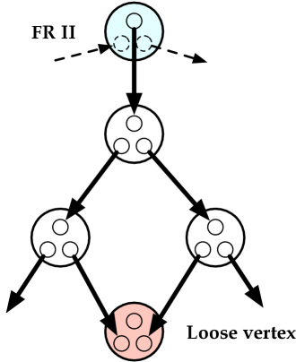
Figure 4: Example of the Phase $3$ branching process. A loose vertex is generated when it is hit twice by a previous generation.

We define $\lambda$ to be the expected number of children. We will show,

Lemma 8.5.

With high probability, $\lambda<1$ in all phase $3$ rounds.

This implies the key Lemma 8.1.

Proof of Lemma 8.1.

If $\lambda<1$ in all rounds, then standard results on branching processes imply that the probability any particular round processes more than $O(\log n)$ vertices is $O(1/n^{2})$, for appropriate choices of constants. A union bound then implies that the probability all of them process $O(\log n)$ vertices is at least $1-1/n$.

This assumption on $\lambda$ holds w.h.p. by Lemma 8.5, completing the proof. ∎

Analysis of the Branching Process: Proof of Lemma 8.5.

We will use the method of differential equations [30] to establish Lemma 8.5. All the required Lipchitz conditions and tail bounds in our process are easy to check, since the degree sequence is asymptotically Poisson. Thus the main step is to define and analyze the system of differential equations describing the evolution of the degree sequence as the algorithm runs.

In order to simplify the analysis, we break the loop into individual timesteps. At each timestep, two vertex copies are removed from $\mathcal{A}_{s}$. For example, the step 1 of the algorithm is divided into $deg_{\mathcal{A}_{s}}(v)$ many timesteps, where in each timestep we remove a copy of $v$ and another random copy. Similarly, step 3 of the algorithm gets divided into $deg_{\mathcal{A}_{s}}(v)-3$ many timesteps.

For all $i\geq 3$, let $a^{(i)}$ denote the number of vertices of degree $i$ in the $3$-core divided by $n$ (where $n$ is the number of vertices in $G=G(n,c/n)$). We say a vertex is hit during a round in phase 3 if a copy of the vertex is selected by step 1(b) of the algorithm during the round. Since in phase $3$ vertices of degree $4$ and greater get hit randomly with probability proportional to their degree, they always obey a truncated Poisson distribution. Therefore, for $i\geq 4$, $a^{(i)}$ will be a truncated Poisson distribution with a time-varying mean $\delta$,

(8.1) $$a^{(i)}=\frac{\mathrm{e}^{-\delta}\,\delta^{i}}{i!}\,.$$

Let $\mu$ denote the total number of vertex copies in the $3$-core divided by $n$. That is,

$$\begin{split}\mu=\sum_{i\geq 3}ia^{(i)}=3a^{(3)}+\sum_{i\geq 4}\frac{\mathrm{e}^{-\delta}\,\delta^{i}}{(i-1)!}\\ =3a^{(3)}+\delta\left(1-\mathrm{e}^{-\delta}\left(1+\delta+\frac{\delta^{2}}{2}\right)\right)\,.\end{split}$$

We will use the following notation for the number of copies of degree $j$ or greater divided by $n$, $\mu^{\geq j}=\sum_{i=j}^{\infty}ia^{(i)}\,.$

Since an edge hits a vertex of degree $3$ with probability $3a^{(3)}/\mu$, and since it creates two new edges when it does so, the branching ratio of the branching process defined above is $\lambda=6a^{(3)}/\mu.$ To show that the branching process is subcritical we need to analyze $\lambda$ and show that throughout phase $3$ it is bounded away from $1$.

Now, in one timestep the expected change in $a^{(i)}$ ($i\geq 4$) is

$$n\cdot\mathbb{E}[\Delta a^{(i)}]=\frac{(i+1)a^{(i+1)}}{\mu}-\frac{ia^{(i)}}{\mu}\,.$$

Here, the first term on the right hand side represents the probability that a degree $i+1$ vertex is hit (this creates a new degree $i$ vertex). The second term represents the probability that a degree $i$ vertex is hit (this destroys a degree $i$ vertex). Similarly, the expected change in $a^{(3)}$ in one timestep is

$$n\cdot\mathbb{E}[\Delta a^{(3)}]=\frac{4a^{(4)}}{\mu}-\frac{3a^{(3)}}{\mu}-(1-\lambda)\,.$$

Here, the additional $1-\lambda$ term comes due to the FR II step. The expected probability on a given timestep that there are no degree-$2$ vertices is $1-\lambda$.

Setting the derivatives of these variables to their expectations gives us our differential equations:

$$n\cdot\frac{\mathrm{d}a^{(3)}}{\mathrm{d}t}=\frac{-3a^{(3)}+4a^{(4)}}{\mu}-(1-\lambda)$$

and, for all $i\geq 4$

$$n\cdot\frac{\mathrm{d}a^{(i)}}{\mathrm{d}t}=\frac{-ia^{(i)}+(i+1)a^{(i+1)}}{\mu}$$

Changing the variable of integration to $s$ where $\mathrm{d}s/\mathrm{d}t=1/(n\mu)$ and substituting $\lambda=6a^{(3)}/\mu$ gives

(8.2) $$\frac{\mathrm{d}a^{(3)}}{\mathrm{d}s} =-3a^{(3)}+4a^{(4)}-\mu+6a^{(3)}=-\mu^{\geq 5}$$

(8.3) $$\frac{\mathrm{d}a^{(i)}}{\mathrm{d}s} =-ia^{(i)}+(i+1)a^{(i+1)}\quad\mbox{for all $i\geq 4$}\,.$$

This infinite system is consistent with the truncated Poisson form for $a^{(i)}$. Since (8.1) implies

$$\frac{\mathrm{d}a^{(i)}}{\mathrm{d}s}=\left(\frac{i}{\delta}-1\right)a^{(i)}\,\frac{\mathrm{d}\delta}{\mathrm{d}s}\;\;\mbox{ and }\;\;a^{(i+1)}=\frac{\delta}{i+1}\,a^{(i)}\,,$$

Equation (8.3) becomes

$$\left(\frac{i}{\delta}-1\right)a^{(i)}\,\frac{\mathrm{d}\delta}{\mathrm{d}s}=(-i+\delta)a^{(i)}\;\;\mbox{ or }\;\;\frac{\mathrm{d}\delta}{\mathrm{d}s}=-\delta\,.$$

Thus, $\delta$ as a function of $s$ is, $\delta=\delta_{0}\,\mathrm{e}^{-s}$. Here, $\delta_{0}$ is the parameter of the truncated Poisson distribution describing the degree distribution of the $3$-core. We can also express $\mu$ as a function of $s$. Since $\lambda=6a^{(3)}/\mu$, we can also express $\lambda$ as a function of $s$. Then we show using analytic arguments that $\lambda<1$ for all values of $s$ in phase $3$.

We start by computing the integral,

$$a^{(3)}=a^{(3)}_{0}-\int_{0}^{s}\mu^{\geq 5}\,\mathrm{d}s,$$

analytically. Since $\frac{\mathrm{d}\delta}{\mathrm{d}s}=-\delta$, we have $\mathrm{d}s=\frac{-\mathrm{d}\delta}{\delta}$. Let $\delta_{0}=\tau$. Remember, $\delta_{0}$ is the parameter of the truncated Poisson distribution describing the degree distribution of the $3$-core. Now, $\mu^{\geq 5}$ can be expressed as

$$\mu^{\geq 5}=\sum_{i=5}^{\infty}\frac{\mathrm{e}^{-\delta}\delta^{i}}{(i-1)!}=\delta\left(1-\mathrm{e}^{-\delta}\left(1+\delta+\frac{\delta^{2}}{2}+\frac{\delta^{3}}{6}\right)\right).$$

We can compute $a^{(3)}$ as

$$a^{(3)}$$

$$=a^{(3)}_{0}-\int_{0}^{s}\mu^{\geq 5}\,\mathrm{d}s=a^{(3)}_{0}+$$

$$\int_{\tau}^{\tau\mathrm{e}^{-s}}\delta\left(1-\mathrm{e}^{-\delta}\left(1+\delta+\frac{\delta^{2}}{2}+\frac{\delta^{3}}{6}\right)\right)\frac{\mathrm{d}\delta}{\delta}$$

$$=a^{(3)}_{0}+\int_{\tau}^{\tau\mathrm{e}^{-s}}\left(1-\mathrm{e}^{-\delta}\left(1+\delta+\frac{\delta^{2}}{2}+\frac{\delta^{3}}{6}\right)\right)\mathrm{d}\delta$$

$$=a^{(3)}_{0}+\tau\mathrm{e}^{-s}+\mathrm{e}^{-\tau\mathrm{e}^{-s}}\left(\frac{\tau^{3}\mathrm{e}^{-3s}}{6}+\tau^{2}\mathrm{e}^{-2s}+3\tau\mathrm{e}^{-s}+4\right)$$

$$-\left(\tau+\frac{\tau^{3}\mathrm{e}^{-\tau}}{6}+\tau^{2}\mathrm{e}^{-\tau}+3\tau\mathrm{e}^{-\tau}+4\mathrm{e}^{-\tau}\right).$$

Now, $a^{(3)}_{0}=\mathrm{e}^{-\tau}\tau^{3}/6$. Therefore, $a^{(3)}$ as a function of $s$ is

$$a^{(3)}$$

$$=\frac{\mathrm{e}^{-\tau}\tau^{3}}{6}+\tau\mathrm{e}^{-s}+\mathrm{e}^{-\tau\mathrm{e}^{-s}}(\frac{\tau^{3}\mathrm{e}^{-3s}}{6}+\tau^{2}\mathrm{e}^{-2s}+3\tau\mathrm{e}^{-s}+4)$$

$$-\left(\tau+\frac{\tau^{3}\mathrm{e}^{-\tau}}{6}+\tau^{2}\mathrm{e}^{-\tau}+3\tau\mathrm{e}^{-\tau}+4\mathrm{e}^{-\tau}\right).$$

Since both $a^{(3)}$ and $\delta$ can be expressed as a function of $s$, we can write

$$\mu$$

$$=3a^{(3)}+\delta\left(1-\mathrm{e}^{-\delta}\left(1+\delta+\frac{\delta^{2}}{2}\right)\right)$$

$$=3\left(\frac{\mathrm{e}^{-\tau}\tau^{3}}{6}+\tau\mathrm{e}^{-s}\right)$$

$$+3\left(\mathrm{e}^{-\tau\mathrm{e}^{-s}}\left(\frac{\tau^{3}\mathrm{e}^{-3s}}{6}+\tau^{2}\mathrm{e}^{-2s}+3\tau\mathrm{e}^{-s}+4\right)\right)$$

$$-3\left(\tau+\frac{\tau^{3}\mathrm{e}^{-\tau}}{6}+\tau^{2}\mathrm{e}^{-\tau}+3\tau\mathrm{e}^{-\tau}+4\mathrm{e}^{-\tau}\right)$$

$$+\tau\mathrm{e}^{-s}\left(1-\mathrm{e}^{-\tau\mathrm{e}^{-s}}\left(1+\tau\mathrm{e}^{-s}+\frac{\tau^{2}\mathrm{e}^{-2s}}{2}\right)\right),$$

as a function of $s$. Now, given $a^{(3)}$ and $\mu$ as functions of $s$, we can compute $\lambda=6a^{(3)}/\mu$ as a function of $s$. We need to show that $\lambda<1$ for all values of $s\geq 0$ in phase $3$. Let $s^{*}$ be the value of $s$ at which $a^{(3)}$ (as a function of $s$) evaluates to $0$ (this signals the end of phase 3). By taking derivatives, it can be shown that $\lambda$ is a decreasing function of $s$ in the interval $(0,s^{*})$ (we omit this calculation here). So, all left to verify is whether at $s=0$, $\lambda<1$. Evaluating $\lambda$ at $s=0$, we get

$$\lambda|_{s=0}=\frac{6\cdot\frac{\mathrm{e}^{-\tau}\tau^{3}}{6}}{\frac{3\mathrm{e}^{-\tau}\tau^{3}}{6}+\tau-\mathrm{e}^{-\tau}(\tau+\tau^{2}+\frac{\tau^{3}}{2})}=\frac{\mathrm{e}^{-\tau}\tau^{2}}{1-\mathrm{e}^{-\tau}(1+\tau)}.$$

For $\tau>1.794$, $\lambda|_{s=0}<1$. At the birth of the giant rigid component $(c=c_{2}\approx 3.58804)$, $\tau=2.688$, and as we increase $c$, the value of $\tau$ only increases. Therefore, for all $c>c_{2}$, $\lambda|_{s=0}<1$. As, $\lambda$ is a decreasing function of $s$, therefore for $c>c_{2}$, $\lambda<1$ throughput phase $3$. This shows that for $c>c_{2}$ all branching processes in phase $3$ are subcritical.

∎

9 Conclusions

We studied the emergence of rigid components in sparse Erdős-Rényi random graphs, proving that there is a sharp threshold and a quantitative bound on the size of the rigid component when it emerges. These results confirm theoretically the simulations of [24].

As conjectures, we leave the following:

Conjecture 9.1.

With high probability, the entire $(3+2)$-core is Laman-spanning in $G(n,c/n)$, for $c>c_{2}$.

Conjecture 9.2.

With high probability, the $3$-core of $G(n,c/n)$ is globally rigid (i.e., there is exactly one embedding of the framework’s edge lengths, as opposed to a discrete set), for $c>c_{2}$.

In the plane, generic global rigidity is characterized by the framework’s graph being $3$-connected and remaining Laman-spanning if any edge is removed [6]. Proving either of these conjectures using the plan presented here would most likely require a stronger statement than Theorem 1.2, such as the $3$-core being, w.h.p., $(2,0)$-spanning.

Conjecture 9.3.

With high probability, the size of the $(3+2)$-core when it emerges is given by $qn$, where $q$ is the root of the equation $q=1-\mathrm{e}^{-qc}(1+qc)$.

The term $\mathrm{e}^{-qc}(1+qc)$ comes from $\Pr[Po(qc)<2]$. This conjecture, with Theorem 1.1, implies that when the giant rigid component emerges it spans about $0.749n$ vertices.

Acknowledgements.

We would like to thank Michael Molloy, Alexander Russell, and Lenka Zdeborovà for initial discussions. We would also like to thank Daniel Fernholz and Vijaya Ramachandran for discussions regarding [8].

References

- [1] EA Bender and ER Canfield. The asymptotic number of labeled graphs with given degree sequences. Journal of Combinatorial Theory, Series A, 24(3):296–307, 1978.
- [2] B Bollobás. A probabilistic proof of an asymptotic formula for the number of labelled regular graphs. Journal européen de combinatoire, 2:311, 1980.
- [3] B Bollobás. Random graphs. Cambridge Studies in Advanced Mathematics, 2001.
- [4] Julie Anne Cain, Peter Sanders, and Nick Wormald. The random graph threshold for k-orientiability and a fast algorithm for optimal multiple-choice allocation. In SODA, pages 469–476. Society for Industrial and Applied Mathematics, 2007.
- [5] M V Chubynsky and Michael F Thorpe. Rigidity percolation and the chemical threshold in network glasses. J.Optoelectron.Adv.Mater, pages 229–240, 2002.
- [6] Robert Connelly. Generic global rigidity. Discrete Comput. Geom., 33(4):549–563, 2005.
- [7] C Cooper. The cores of random hypergraphs with a given degree sequence. Random Structures and Algorithms, 25(4):353–375, 2004.
- [8] Daniel Fernholz and Vijaya Ramachandran. The -orientability thresholds for . In SODA ’07: Proceedings of the eighteenth annual ACM-SIAM symposium on Discrete algorithms, pages 459–468. Society for Industrial and Applied Mathematics, 2007.
- [9] Jack Graver, Brigitte Servatius, and Herman Servatius. Combinatorial rigidity. Amer Mathematical Society, 1993.
- [10] Ruth Haas, Audrey Lee, Ileana Streinu, and Louis Theran. Characterizing sparse graphs by map decompositions. Journal of Combinatorial Mathematics and Combinatorial Computing, 62:3–11, 2007.
- [11] L. Henneberg. Die graphische Statik der starren Systeme. BG Teubner, 1911.
- [12] Bill Jackson, Brigitte Servatius, and Herman Servatius. The 2-dimensional rigidity of certain families of graphs. Journal of Graph Theory, 54(2):154–166, 2007.
- [13] Donald J Jacobs and Bruce Hendrickson. An algorithm for two-dimensional rigidity percolation: the pebble game. Journal of Computational Physics, 137:346–365, 1997.
- [14] Donald J Jacobs and Michael F Thorpe. Generic rigidity percolation: The Pebble Game. Physical review letters, 75(22):4051–4054, 1995.
- [15] S Janson and MJ Luczak. A simple solution to the k-core problem. Random Structures and Algorithms, 30(1-2):50–62, 2007.
- [16] Gerard Laman. On graphs and rigidity of plane skeletal structures. J. Engrg. Math., 4:331–340, 1970.
- [17] Audrey Lee and Ileana Streinu. Pebble game algorihms and sparse graphs. Discrete Math., 308(8):1425–1437, Apr 2008.
- [18] J Maxwell. L. on the calculation of the equilibrium and stiffness of frames. Philosophical Magazine Series 4, Jan 1864.
- [19] M. Molloy. The pure literal rule threshold and cores in random hypergraphs. In SODA, pages 672–681, 2004.
- [20] M Molloy and B Reed. A critical point for random graphs with a given degree sequence. Random Structures and Algorithms, 6(2-3):161–180, 1995.
- [21] M Molloy and B Reed. The size of the giant component of a random graph with a given degree sequence. Combin. Probab. Comput, 7:295–306, 1998.
- [22] C.F. Moukarzel. Rigidity percolation in a field. Physical Review E, 68(5):56104, 2003.
- [23] Boris Pittel, Joel Spencer, and Nicholas Wormald. Sudden emergence of a giant k-core in a random graph. J. Comb. Theory Ser. B, 67(1):111–151, 1996.
- [24] O. Rivoire and J. Barré. Exactly solvable models of adaptive networks. Physical review letters, 97(14):148701, 2006.
- [25] Ileana Streinu. Personal communication.
- [26] Ileana Streinu and Louis Theran. Slider-pinning rigidity: a maxwell-laman-type theorem. Discrete Comput. Geom., 44(4):812–837, 2010.
- [27] Louis Theran. Rigid components of random graphs. Proceedings of CCCG’09, 2009.
- [28] Michael F Thorpe and M V Chubynsky. Self-organization and rigidity in network glasses. Current Opinion in Solid State & Materials Science, 5:525–532, 2002.
- [29] Michael F Thorpe, Donald J Jacobs, M V Chubynsky, and A J Rader. Generic rigidity of network glasses. In Rigidity theory and applications, pages 239–277. Springer, 2002.
- [30] Nicholas C Wormald. Differential equations for random processes and random graphs. Ann. Appl. Probab., 5(4):1217–1235, 1995.