An extension of gas-kinetic BGK Navier-Stokes scheme to multidimensional astrophysical magnetohydrodynamics

Abstract

The multidimensional gas-kinetic scheme for the Navier-Stokes equations under gravitational fields [J. Comput. Phys. 226 (2007) 2003-2027] is extended to resistive magnetic flows. The non-magnetic part of the magnetohydrodynamics equations is calculated by a BGK solver modified due to magnetic field. The magnetic part is treated by the flux splitting method based gas-kinetic theory [J. Comput. Phys. 153 (1999) 334-352 ], using a particle distribution function constructed in the BGK solver. To include Lorentz force effects into gas evolution stage is very important to improve the accuracy of the scheme. For some multidimensional problems, the deviations tangential to the cell interface from equilibrium distribution are essential to keep the scheme robust and accurate. Besides implementation of a TVD time discretization scheme, enhancing the dynamic dissipation a little bit is a simply and efficient way to stabilize the calculation. One-dimensional and two-dimensional shock waves tests are calculated to validate this new scheme. A three-dimensional turbulent magneto-convection simulation is used to show the applicability of current scheme to complicated astrophysical flows.

1 Introduction

Plasma is a very common phase of matter in the universe, especially under astrophysical circumstances. For instance, star can be regarded as very hot ball of plasma. The solar surface activities are thought to be tightly related to the interaction between turbulent convection and magnetic flux tubes. The accretion flows are always magnetized. Magnetic fields are also important in the interstellar medium of spiral, barred and irregular galaxies. These problems usually are complicated and high-nonlinear. Along with the fast growth of computer power, numerical computation is becoming a more and more popular way to study them.

During the past decades, to meet the demands of industrial design and scientific computation, a lot of efforts have been made to develop accurate and robust numerical schemes for supersonic flows. Various methods, such as Godnov scheme, piecewise parabolic method (PPM)[3], total variation diminishing (TVD) scheme[6] and gas-kinetic BGK scheme[21, 20], have been invented based on different philosophies. When calculating the shock waves, we face the dilemma of keeping accuracy or robustness. In order to stabilize the calculation, we need dissipation. While an unnecessary dissipation would reduce the accuracy of the scheme. Hence, the capability of a shock-capturing scheme depends on how smart the introduction of the numerical dissipation is. In the gas-kinetic BGK scheme, this is done by particle collisions. Due to collision, the particles will approach a thermally equilibrium state, e.g., Maxwellian distribution. Practice shows that this is a smart way to control dissipation. The resulted supersonic flow solver is accurate and robust.

At the same time, some schemes for magnetohydrodynamics (MHD) have been developed or extended from their hydrodynamics (HD) version. For example, the PPM has been extended to mulitdimensional MHD by Dai and Woodward[4]. They also proposed an approximate MHD Riemann solver and an approach to maintain the divergence free condition of magnetic field[5]. A second-order accurate TVD Roe-type upwind MHD scheme and its multidimensional version were presented in [8, 9]. Most of them are based on characteristic decomposition. Because of the non-strictly hyperbolicity of the MHD system, it is hard to validate the MHD eigensystem. The gas-kinetic theory based flux splitting method for ideal MHD developed by Xu[19] is a robust and first-order scheme. It was extended to higher order and multidimensional by Tang and Xu[14]. Without wave decomposition, it is an efficient scheme. For the flux vector splitting (FVS) schemes[13], the flux function is split to $F=F^{+}+F^{-}$, where the numerical dissipation is proportional to the numerical resolution. An equilibrium part due to particle collisions is introduced in [19], i.e., $F=(1-\alpha)F^{e}+\alpha(F^{+}+F^{-})$. $\alpha\in[0,1]$ is an adjustable parameter used to control the particle collisions. In doing so, the unnecessary numerical viscosity is reduced.

For the BGK-Navier-Stokes (BGK-NS) solver, the particle collisions are controlled by the solution of BGK equation[1] instead of an arbitrary parameter. The reduction of dissipation only takes place where it is physically necessary. In oder to apply the BGK-NS solver to astrophysical flows, the magnetic field has to be included. The problem is that an implementation of the magnetic terms with arbitrary descretization scheme might give rise to complicated truncation error behaviour. As analyzed by [17], it is better to use the same difference operator to discretize all the terms in the equations, otherwise, the interaction between different kinds of truncation errors would introduce unphysical effect, e.g., numerical heating or numerical dispersion. In the current study, the non-magnetic part of MHD equations is solved by BGK-NS scheme, the magnetic part is solved by flux splitting method based on the solution of BGK equation.

This paper is organized as follows. Section 2 describes the extension of BGK scheme to include magnetic field. In Section 3 numerical experiments are performed to validate the current scheme. Section 4 discusses selected problems related to the current scheme and some general issues of developing MHD scheme. Section 5 is the conclusion.

2 Numerical Scheme

In this section, I describe a scheme for solving the following resistive MHD equations under gravitational field:

$$\partial\rho/\partial t = -\nabla\cdot\rho\vec{v},$$ (1)

$$\partial\rho\vec{v}/\partial t = -\nabla\cdot(\rho\vec{v}\vec{v}-\vec{B}\vec{B})-\nabla p_{\rm tot}+\nabla\cdot\vec{\Sigma}+\rho(-\nabla\phi),$$ (2)

$$\partial E/\partial t = -\nabla\cdot[(E+p_{\rm tot})\vec{v}-\vec{v}\cdot\vec{\Sigma}+\vec{F}_{\rm d}-\vec{B}\vec{B}\cdot\vec{v}-\vec{B}\times\eta(\nabla\times\vec{B})]+\rho\vec{v}\cdot(-\nabla\phi),$$ (3)

$$\partial\vec{B}/\partial t = -\nabla\cdot(\vec{v}\vec{B}-\vec{B}\vec{v}-\eta\nabla\vec{B})$$ (4)

where, $p_{\rm tot}=p_{g}+p_{m}$, $E=E_{i}+E_{m}+E_{k}$, $p_{g}$ is the gas pressure, $p_{m}=\frac{1}{2}\vec{B}\cdot\vec{B}$ is the magnetic pressure, $E_{i}$ is the internal energy, $E_{m}=\frac{1}{2}\vec{B}\cdot\vec{B}$ is the magnetic energy and $E_{k}=\frac{1}{2}\rho v^{2}$ is the kinetic energy. $(-\nabla\phi)$ is the gravitational acceleration, $F_{d}$ the diffusive heat flux, $\vec{\Sigma}$ the viscous stress tensor, $\eta$ the magnetic resistivity. All the other symbols have their standard meaning. The above equations can be written in a compact form:

$$\frac{\partial U}{\partial t}=\frac{\partial F_{x}}{\partial x}+\frac{\partial F_{y}}{\partial y}+\frac{\partial F_{z}}{\partial z}+Q$$ (5)

where $U=(\rho,\rho\vec{v},\vec{B},E)^{T}$ and $Q=(0,\rho(-\nabla\phi),0,\rho\vec{v}\cdot(-\nabla\phi))^{T}$ are cell averaged quantities. $F_{x}$, $F_{y}$ and $F_{z}$ are defined on the cell interface. In each direction, the fluxes can be split into two parts. For example, $F_{x}$ can be further written as $F_{x}=F_{x,\rm{bgk}}+F_{x,\rm{split}}$, where

$$F_{x,\rm bgk}=-\left(\begin{array}[]{c}\rho v_{x}\\ \rho v_{x}v_{x}+p_{tot}-\Sigma_{x}\\ \rho v_{x}v_{y}-\Sigma_{y}\\ \rho v_{x}v_{z}-\Sigma_{z}\\ 0\\ 0\\ 0\\ (E+p_{\rm tot})v_{x}-\kappa\nabla_{x}T-v_{x}\Sigma_{x}\end{array}\right),$$ (14)

and

$$F_{x,\rm split}=\left(\begin{array}[]{c}0\\ B_{x}B_{x}\\ B_{x}B_{y}\\ B_{x}B_{z}\\ \eta\nabla_{x}B_{x}\\ B_{x}v_{y}-v_{x}B_{y}+\eta\nabla_{x}B_{y}\\ B_{x}v_{z}-v_{x}B_{z}+\eta\nabla_{x}B_{z}\\ B_{x}(B_{y}v_{y}+B_{z}v_{z}+B_{x}v_{x})+\eta[\vec{B}\times(\nabla\times\vec{B})]_{x}\end{array}\right).$$ (23)

We discretize the non-magnetic part $F_{x,\rm bgk}$ by gas-kinetic BGK scheme, magnetic part $F_{x,\rm split}$ by gas-kinetic theory based flux splitting method.

2.1 A BGK-NS solver for the non-magnetic part

The current scheme calculates $F_{x,\rm{bgk}}$ by the BGK-NS solver [17], which is needed to be modified to take into account the effects of magnetic field. First, the total pressure includes magnetic pressure, and total energy magnetic energy. Secondly, the effects of Lorentz force are added into the BGK equation[1], i.e.,

$$\frac{\partial f}{\partial t}+\vec{c}\cdot\nabla{f}+(-\nabla\phi+\vec{F}_{Lorenzt})\cdot\nabla_{\vec{c}}f=\frac{g-f}{\tau},$$ (24)

where $f(t,x,y,z,c_{x},c_{y},c_{z},\xi)$ is the particle distribution function defined on phase space, $g$ is the Maxwellian distribution,

$$g=\rho\left(\frac{\lambda}{\pi}\right)^{\frac{N+3}{2}}e^{-\lambda((\vec{c}-\vec{v})\cdot(\vec{c}-\vec{v})+\xi^{2}+\vec{B}\cdot\vec{B}/2)},$$ (25)

$\tau$ is relaxation time, $\vec{c}=(c_{x},c_{y},c_{z})$ is the particle micro velocity. $\xi$ is the internal variable, which has $N$ internal degree of freedom. The value of $N$ is determined by the configuration of molecules. $\lambda$ is related to the gas temperature by $\lambda=m/2kT$, $m$ is the molecules mass, $k$ is the Boltzmann constant, and $T$ is the temperature. $\vec{F}_{Lorentz}=\vec{B}\times(\nabla\times\vec{B})/\rho$ is the acceleration due to Lorentz force. Equation (24) has a local approximate solution at cell interface[17]:

$$f= \{(1-e^{-t/\tau})+(e^{-t/\tau}(t+\tau)-\tau)[(\bar{a}_{n}^{l}c_{n}+\bar{b}_{n}^{l}({-\nabla\phi}+\vec{F}_{Lorentz})_{n})H[c_{n}]$$ (26)

$$+(\bar{a}_{n}^{r}c_{n}+\bar{b}_{n}^{r}({-\nabla\phi}+\vec{F}_{Lorentz})_{n})(1-H[c_{n}])$$

$$+\bar{\vec{a}}_{t}\cdot\vec{c}_{t}+\bar{\vec{b}}_{t}\cdot({-\nabla\phi}+\vec{F}_{Lorentz})_{t}]+[t-\tau(1-e^{-t/\tau})]\bar{A}\}g_{0}$$

$$+ e^{-t/\tau}\{[1-\vec{a}^{l}\cdot\vec{c}t-\vec{b}^{l}\cdot({-\nabla\phi}+\vec{F}_{Lorentz})t$$

$$-\tau(\vec{a}^{l}\cdot\vec{c}+\vec{b}^{l}\cdot({-\nabla\phi}+\vec{F}_{Lorentz})+A^{l})]H[c_{n}]g_{0}^{l}$$

$$+ [1-\vec{a}^{r}\cdot\vec{c}t-\vec{b}^{r}\cdot({-\nabla\phi}+\vec{F}_{Lorentz})t$$

$$-\tau(\vec{a}^{r}\cdot\vec{c}+\vec{b}^{r}\cdot({-\nabla\phi}+\vec{F}_{Lorentz})+A^{r})](1-H[c_{n}])g_{0}^{r}\},$$

where the Heaviside function $H[x]$ is defined by

$$H[x]=\left\{\begin{array}[]{l}0,x<0,\\ 1,x\geq 0,\end{array}\right.$$

$x=0$ is the location of cell interface. For a vector defined on the cell interface, its components are grouped into two categories, the component normal to the cell interface and those tangential components. For instance, for velocity $\vec{c}$, $c_{n}$ is the normal component, $\vec{c_{t}}$ are the tangential components. See Fig. 1 for an example. $\bar{\vec{a}}^{l}=[\bar{a}_{n}^{l},\bar{\vec{a}}_{t}^{l}]$, $\vec{a}^{l}=[a_{n}^{l},\vec{a}_{t}^{l}]$, $\bar{\vec{b}}^{l}=[\bar{b}_{n}^{l},\bar{\vec{b}}_{t}^{l}]$, $\vec{b}^{l}=[b_{n}^{l},\vec{b}_{t}^{l}]$, $\bar{\vec{a}}^{r}=[\bar{a}_{n}^{r},\bar{\vec{a}}_{t}^{r}]$, $\vec{a}^{r}=[a_{n}^{r},\vec{a}_{t}^{r}]$, $\bar{\vec{b}}^{r}=[\bar{b}_{n}^{r},\bar{\vec{b}}_{t}^{r}]$, $\vec{b}^{r}=[b_{n}^{r},\vec{b}_{t}^{r}]$, $A^{l}$, $A^{r}$ and $\bar{A}$ are the coefficients measuring the deviations from Maxwellian due to various effects. Calculation of these coefficients is one of the key part of BGK scheme. The details are presented in [17]. The way that current scheme including magnetic field does not affect these calculations. $g_{0}$, $g_{0}^{l}$, $g_{0}^{r}$ are equilibrium and split Maxwellian, respectively. Once the solution of BGK is found, the fluxes of conservative quantities through the cell interface can be obtained, i.e.,

$$F_{x,\rm{bgk}} = -\int c_{x}f\vec{\psi}d\Xi,$$ (28)

$$\vec{\psi} = [1,\vec{c},0,0,0,\frac{1}{2}(\vec{c}\cdot\vec{c}+\xi^{2}+\vec{B}\cdot\vec{B})]^{T},$$ (29)

where $d\Xi=dc_{x}dc_{y}dc_{z}d\xi$ is the volume element in phase space. The above integrals can be worked out analytically, which involves another key part of the BGK scheme – calculation of the moments of Maxwellian. The formula needed can be found in the appendix of [19] or [17].

Figure 1: Two adjacent finite volumes – cells. (i,j) are the cell indices. Dashed lines are the cell interfaces. Fluxes of the conservative quantities, eg., $F_{x}$ and $F_{y}$ are calculated at the cell boundaries. The cell-averaged $U_{i,j}$ is updated every time step. Solid lines show schematically the distribution of magnetic field constructed by van Leer limiter around cell interface if there is a shock. Arrows are a vector and its normal and tangential components.

2.2 A flux splitting solver for the magnetic part

In order to perform the flux splitting, the solution of BGK equation obtained in previous section has to be split into left-side and right-side status, i.e.,

$$f^{l}(c_{n}>0)= \{1+(e^{-t/\tau}(t+\tau)-\tau)[(\bar{a}_{n}^{l}c_{n}+\bar{b}_{n}^{l}({-\nabla\phi}+\vec{F}_{Lorentz})_{n})$$ (30)

$$+\bar{\vec{a}}_{t}^{l}\cdot\vec{c}_{t}+\bar{\vec{b}}_{t}^{l}\cdot({-\nabla\phi}+\vec{F}_{Lorentz})_{t}]+[t-\tau(1-e^{-t/\tau})]\bar{A}$$

$$+ e^{-t/\tau}[\vec{a}^{l}\cdot\vec{c}t+\vec{b}^{l}\cdot({-\nabla\phi}+\vec{F}_{Lorentz})t$$

$$+\tau(\vec{a}^{l}\cdot\vec{c}+\vec{b}^{l}\cdot({-\nabla\phi}+\vec{F}_{Lorentz})+A^{l})]\}g_{0}^{l},$$

$$f^{r}(c_{n}\leq 0)= \{1+(e^{-t/\tau}(t+\tau)-\tau)[(\bar{a}_{n}^{r}c_{n}+\bar{b}_{n}^{r}({-\nabla\phi}+\vec{F}_{Lorentz})_{n})$$ (31)

$$+\bar{\vec{a}}_{t}^{r}\cdot\vec{c}_{t}+\bar{\vec{b}}_{t}^{r}\cdot({-\nabla\phi}+\vec{F}_{Lorentz})_{t}]+[t-\tau(1-e^{-t/\tau})]\bar{A}$$

$$+ e^{-t/\tau}[\vec{a}^{r}\cdot\vec{c}t+\vec{b}^{r}\cdot({-\nabla\phi}+\vec{F}_{Lorentz})t$$

$$+\tau(\vec{a}^{r}\cdot\vec{c}+\vec{b}^{r}\cdot({-\nabla\phi}+\vec{F}_{Lorentz})+A^{r})]\}g_{0}^{r},$$

Two points need to be remarked on the above splitting.

1. The tangential derivations due to derivatives and accelerations are very important for the BGK-NS solver. However, they do not affect the magnetic part evidently. This property seems case-dependent. For example, for the Orzang-Tang vortex problem, including tangential deviations is little bit dispersive. While for the cloud-shock interaction problem, it essentially improve the ability of the scheme. See Section 3 for the details.

2. The right-hand side of Equation (26) consists three parts, i.e., equilibrium part $[\cdots]g_{0}$, split parts $[\cdots]g_{0}^{l}$ and $[\cdots]g_{0}^{r}$. The left and right parts introduce kinematic dissipation to stabilize calculation of discontinuity; while the equilibrium part reduces the kinematic dissipation to an appropriate value, thus improve the accuracy of the numerical scheme. These three terms together form a distribution which would approach an equilibrium state due to the particle collision. If we split the distribution (26) into three parts accordingly, and replace those squares with an adjustable constant $\alpha,(0\leq\alpha\leq 1)$, i.e., $(1-\alpha)g_{0}$, $\alpha g_{0}^{l}$ and $\alpha g_{0}^{r}$, then the following fluxes construction is the same as in method [19]. However, numerical experiment shows that this kind of splitting seems too dispersive, even without substituting those coefficients. This will be discussed further in Section 4.

Using the above split particle distribution, the magnetic part of fluxes can be split as: $F_{x,\rm{split}}=F_{x}^{l}+F_{x}^{r}$. $F_{x}^{l}$ is computed as follows,

$$F_{x}^{l}= \frac{1}{\rho^{l}}\int^{\infty}_{0}f^{l}_{s}\left(\begin{array}[]{c}0\\ B_{x}^{l}B_{x}^{l}\\ B_{x}^{l}B_{y}^{l}\\ B_{x}^{l}B_{z}^{l}\\ \eta\nabla_{x}B_{x}^{l}\\ B_{x}^{l}v_{y}^{l}+\eta\nabla_{x}B_{y}^{l}\\ B_{x}^{l}v_{z}^{l}+\eta\nabla_{x}B_{z}^{l}\\ B_{x}^{l}(B_{y}^{l}v_{y}^{l}+B_{z}^{l}v_{z}^{l}+\frac{1}{2}B_{x}^{l}v_{x}^{l})+\eta[\vec{B^{l}}\times(\nabla\times\vec{B^{l}})]_{x}\end{array}\right)d\Xi$$ (40)

$$+ \frac{1}{\rho^{l}}\int^{\infty}_{0}f^{l}c_{x}\left(\begin{array}[]{c}0\\ 0\\ 0\\ 0\\ 0\\ -B_{y}^{l}\\ -B_{z}^{l}\\ \frac{1}{2}B_{x}^{l}B_{x}^{l}\end{array}\right)d\Xi,$$ (49)

where $(B_{x}^{l},B_{y}^{l},B_{z}^{l})$ and $(B_{x}^{r},B_{y}^{r},B_{z}^{r})$ are the magnetic field at the left-hand side and right-hand side of the cell interface, respectively. They are reconstructed at the beginning of each time step at the cell interface.

$$\vec{B}^{l}=\vec{B}_{i}(x_{i})+(x_{i+1/2}-x_{i})L_{i},$$ (50)

$$\vec{B}^{r}=\vec{B}_{i+1}(x_{i+1})-(x_{i+1}-x_{i+1/2})L_{i+1}.$$ (51)

In the above expressions, the van Leer limiter is defined as,

$$L_{i}=S(s_{+},s_{-})\frac{|s_{+}||s_{-}|}{|s_{+}|+|s_{-}|},$$

where $S(s_{+},s_{-})=\mathrm{sign}(s_{+})+\mathrm{sign}(s_{-})$, $s_{+}=(\vec{B}_{i+1}-\vec{B}_{i})/(x_{i+1}-x_{i})$, and $s_{-}=(\vec{B}_{i}-\vec{B}_{i-1})/(x_{i}-x_{i-1})$. $\rho^{l}$ is constructed in the same way. Fig. 1 gives a schematic example for the reconstruction.

$F_{x}^{r}$ is calculated in the similar way, using $f^{r}$ and integrating on the interval $[-\infty,0]$ . $F_{y}$ and $F_{z}$ are obtained by properly permuting indices.

Some points need to be remarked on the above fluxes splitting,

1. The advective magnetic terms are treated to be passively transported by the motions of particles. $v_{y},v_{z}$ in 1D problems and $v_{z}$ in 2D problems are also passively transported. Those non-advective terms are weighted by the particle distribution.

2. Basically, the integrals on the right-hand-side of (49) are separated according to the following rule. If a term explicitly contains the component of velocity norm to the cell interface, eg., $v_{x}$, then $v_{x}$ is replaced by the particle velocity $c_{x}$ and grouped into the second integral. If not, it is grouped into the first integral.

3. An exception of the above rule is the term $v_{x}^{l}B_{x}^{l}B_{x}^{l}$. Because in Eq. (3),we already include the magnetic pressure $p_{m}$ and magnetic energy density $E_{m}$ into the total pressure $p_{tot}$ and total energy $E$. The transported magnetic contributions to $p_{tot}$ and $E$, eg., $v_{x}B_{x}B_{x}$ should be canceled by the terms from $\vec{B}\vec{B}\cdot\vec{v}$ in Eq. (3). The BGK scheme automatically divides $p_{m}$ and $E_{m}$ into two parts, eg., $p_{m}=(v_{x}p_{m}+c_{x}p_{m})/2$. In order to cancel these terms, we split $v_{x}^{l}B_{x}^{l}B_{x}^{l}$ into: $f^{l}c_{x}^{l}B_{x}^{l}B_{x}^{l}/2$ and $f^{l}v_{x}^{l}B_{x}^{l}B_{x}^{l}/2$, accordingly.

2.3 Equation of State

Internal variable $\xi$ is used to take account of the realistic effects of molecular structure to equation of state (EOS). For 3D diatomic molecule ideal gas, $\rho\xi^{2}/2$ is the sum of vibrational and rotational energy. $\xi$ is a function of the effective internal freedom degree $K$. For 3D cases, $K=N$. For 2D cases, $K=N+1$, where the particle’s motion in the additional third direction is included. For 1D problems, $K=N+2$. Instead of temperature $T$ and internal energy $E_{i}$, in the gas evolution stage of the BGK scheme, $\lambda$ and internal freedom degree $K$ are involved explicitly. For non-magnetic ideal gas, they are defined as:

$$\lambda = \frac{\rho}{2p},$$ (52)

$$K = 4(E_{i})\lambda/\rho-3.$$ (53)

For general cases, we define effective $\lambda^{\ast}$ and $K^{\ast}$ as following:

$$\lambda^{\ast} = \frac{\rho}{2p_{tot}},$$ (54)

$$K^{\ast} = 4(E_{tot}-E_{k})\lambda^{\ast}/\rho-3,$$ (55)

where, $p_{tot}=p_{g}+p_{r}+p_{m}$ and $E_{tot}=E_{i}+E_{r}+E_{m}+E_{k}$. $p_{m}$ and $E_{m}$ are the pressure and energy due to magnetic field. $p_{r}$ and $E_{r}$ can be the pressure and energy due to radiation or ionization.

2.4 Controlling Dissipation

Besides MUSCL type of reconstruction, the numerical dissipation can be determined explicitly. The aforementioned collision time is defined as following,

$$\tau=C_{1}\Delta t+C_{2}\frac{|p^{l}_{tot}-p^{r}_{tot}|}{|p^{l}_{tot}+p^{r}_{tot}|}\Delta t+\frac{\mu}{p_{tot}},$$ (56)

where $\Delta t$ is numerical time-step, $\mu$ is the dynamic viscosity, $p^{l}_{tot}$, $p^{r}_{tot}$ are reconstructed total pressure at the left- and right-side of the cell interface. $C_{2}=1$. For viscous flows, $C_{1}=0$, for inviscid flows, $C_{1}=0.1\sim 0.2$. For magnetic flows, usually, the resistivity $\eta$ is set to zero for ideal MHD. Sometimes, a small value of resistivity, e.g., $\eta=0.008\Delta t$ is needed to stabilize the calculation.

2.5 Ensuring $\nabla\cdot\vec{B}=0$

The divergence free condition of magnetic field means the nonexistence of magnetic monopoles. Although in theory, they possibly exist, in reality they have never been found. On the contrary, caused by numerical truncation error, in MHD simulation, non-zero $\nabla\cdot\vec{B}$ is accumulated rapidly during time marching and destroys the physical consistence of the system. In practice, there are different ways to suppress such kind of accumulation. A detailed comparison of these method is given by Tóth [18]. In 8-wave scheme, the non-zero divergence is propagated away. More often, people use projection method to correct $\vec{B}$ obtained from MHD scheme at time-step $n+1$. Through $\vec{B}^{\ast}=\vec{B}^{n+1}+\nabla\Theta$, where $\nabla^{2}\Theta+\nabla\cdot\vec{B}^{n+1}=0$, $\nabla\cdot\vec{B}^{\ast}=0$ is satisfied. Since this method needs solving a Possion equation, it is not very efficient for 3D problems solved on very large grids. In the current study, I use projection method for 2D programs. For 3D programs, I employ the so-called field-interpolated constrained transport scheme [5] to ensure the divergence free constraint. In this method, perfect cancellation of terms makes the divergence unchanging during time marching. It is simply and time saving. After obtaining the cell-averaged $\vec{B}$ at time $t^{n+1}$ by gas kinetic scheme, we have magnetic field at time $t^{n+1/2}$, $\vec{B}^{n+1/2}=0.5(\vec{B}^{n}+\vec{B}^{n+1})$. $\vec{B}^{n+1/2}$ is used to evaluate the right-hand-side of Eq. (57).

$$\frac{\partial\vec{B}}{\partial t}=\nabla\times(\vec{v}\times\vec{B}-\eta\nabla\times\vec{B}).$$ (57)

The left-hand-side of Eq. (57) represents the values on the staggered mesh. After the values on staggered mesh are updated, the new cell-averaged values are obtained though interpolation. In principle, this method can ensure divergence free constraint to machine error. However, the truncation error occurring in boundary ghost cells propagates into the computational domain. Finally, we maintain $\nabla\cdot\vec{B}=0$ to the truncation error.

After the correction of the magnetic field, the total energy should be modified also to make the computation physically consistent, i.e.,

$$E^{n+1}=E^{n+1}-\frac{1}{2}(\vec{B}^{n+1}\cdot\vec{B}^{n+1})+\frac{1}{2}(\vec{B}^{\ast}\cdot\vec{B}^{\ast})$$ (58)

3 Numerical Tests

For all the tests presented in this section, the van Leer limiter is used for the initial reconstruction of the conservative variables. In order to make the comparison as precise as possible, for some problems, a constant numerical time-step is used.

3.1 1D MHD Shock Waves

Figure 2: The MHD shock tube test. A second order TVD Runge-Kutta scheme is used for the time stepping. Dots are the result of the Maxwellian based gas-kinetic flux splitting scheme with $\alpha=0.9$. Lines are the result of the current MHD BGK scheme. The simulations use 400 cells and a time step of $\Delta t=0.2\Delta x$, corresponding to a Courant constant of $\sim 0.78$. A ratio of specific heats $\gamma=2$ is adopted. The plotted quantities are density $\rho$, gas pressure $p_{g}$, total energy density $E$, x-velocity $v_{x}$, y-velocity $v_{y}$ and y-magnetic field $B_{y}$ at $t=0.2$.

Figure 3: The MHD shock tube test. The Euler time-stepping scheme is used. Dots are the result of the current MHD BGK scheme with effects of Lorentz force included in the gas evolution stage. Lines are the result of the MHD BGK scheme without considering Lorentz force in the particle distribution function. The simulations use 400 cells and a time step of $\Delta t=0.2\Delta x$, corresponding to a Courant constant of 0.78. A ratio of specific heats $\gamma=2$ is adopted. The plotted quantities are density $\rho$, gas pressure $p_{g}$, total energy density $E$, x-velocity $v_{x}$, y-velocity $v_{y}$ and y-magnetic field $B_{y}$ at $t=0.2$.

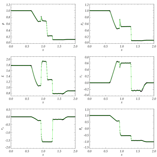
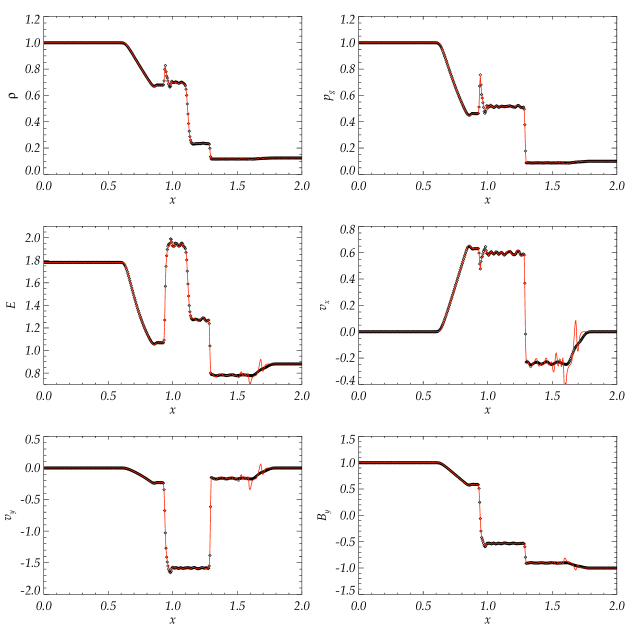
To validate the scheme described in Section 2 and check the effects of Lorentz force in the gas evolution stage, I test the Biro-Wu 1D MHD shock problem[2]. The calculations are performed on $x\in[0,2]$. The initial conditions are set up with the left state $(\rho,v_{x},v_{y},v_{z},p_{g},B_{x},B_{y},B_{z})=(1,0,0,0,1,0.75,1,0)$ and the right state $(0.125,0,0,0,0.1,0.75,-1,0)$. Density $\rho$, gas pressure $p_{g}$, total energy density $E$, x-velocity $v_{x}$, y-velocity $v_{y}$ and y-magnetic field $B_{y}$ at time $t=0.2$ are plotted in Fig. 2 and Fig. 3. When computing the solutions in Fig. 2, a second-order TVD Runge-Kutta scheme[10] is used to do time-marching. The solutions in Fig. 3 are obtained by Euler time-marching scheme. Fig. 2 compares the gas evolutions govern by the Maxwillian or the solution of BGK equation. We can see the stability is increased by using solution of BGK equation. Fig. 3 shows the effect of including the Lorentz force in gas evolution stage. The oscillations between the front of shock and the front of fast wave are greatly suppressed. This kind of suppressing is not obvious in second order time marching scheme, which means that the Lorentz force plays a role of first order time accuracy effects in the gas evolution.

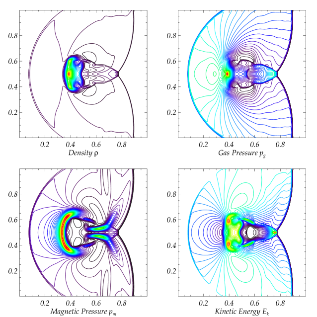
3.2 Spherical Explosion[22]

This test is used to test the influence of strong magnetic field to the shock wave propagation. The computational domain is $[0,1]\times[0,1]$. Initially, the density is 1 everywhere. There is a high pressure region around the center with a radius of $0.1$. The pressure inside and outside the central region are 100 and 1, respectively. The magnetic field is initialized as $(B_{x},B_{y},B_{z})=(0,50/\sqrt{\pi},0)$. The ratio of specific heats $\gamma$ equals 2. A uniform $100\times 100$ mesh is used for this problem. The boundaries are periodic.

Figure 4: A snapshot of the solution to the spherical explosion problem at time $t=0.0105$. The calculation is performed on a uniform mesh of 100 $\times$ 100 grids, using the current BGK MHD scheme. 25 contours for each quantity are plotted. Numerical time step is fixed at $\Delta t=0.008$, corresponding to a Courant number $\approx 0.67$.

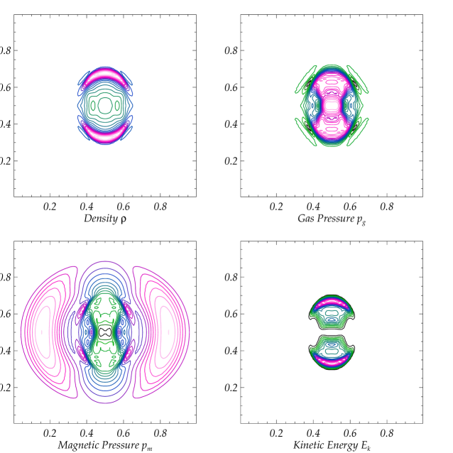
Fig. 4 shows a snapshot of the solution at $t=0.0105$. Density, gas pressure, magnetic pressure and kinetic energy are visualized with 25 contours for each quantities. Due to the strong magnetic field, the spherical explosion are highly anisotropic. The shocks also form in the magnetic field.

Figure 5: The density distributions of the spherical explosion problem along $y=0.5$ at time $t=0.0105$. Solid line is obtained by the current BGK MHD scheme. Dots are from the Maxwellian based gas-kinetic scheme with $\alpha=0.95$.

Fig. 5 compares the density distributions from different scheme. These distributions are taken along $y=0.5$ at time $t=0.0.105$. Solid line is obtained by the current BGK MHD scheme. Dots are from Maxwellian based gas-kinetic scheme with $\alpha=0.95$. The post-shock region indicates that the current scheme is less dissipative than the Maxwellian based scheme.

3.3 Orszag-Tang Turbulent Vortex

Figure 6: A snapshot of the solution to the Orszag-Tang MHD turbulent problem at time $t=3$. The calculation is performed on a uniform mesh of 192 $\times$ 192 grids, using BGK MHD scheme without including the tangential derivatives in the gas evolution stage. 25 contours for each quantity are plotted. Numerical time step is fixed at $\Delta t=0.008$, corresponding to a Courant number $\approx 0.67$.

Figure 7: The density distributions of the Orszag-Tang problem at time $t=3$. (a) Maxwellian based gas-kinetic flux splitting with $\alpha=0.7$; (b) current scheme with Lorentz force switched off in the gas evolution stage; (c) tangential derivates switched on; (d) tangential component of Lorentz force switched on.

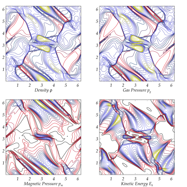
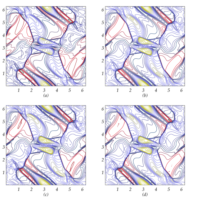
The 2D Orszag-Tang turbulent vortex problem [7] is widely used by computational fluid dynamics (CFD) community to test the MHD scheme because of its complicated interaction between different waves generated as the vortex system evolving. The computations are preformed on a domain of $[0:2\pi]\times[0:2\pi]$. The initial conditions are

$$\rho(x,y)=\gamma^{2},u_{x}=-\sin{(y)},u_{y}=\sin{(x)},$$

$$p_{g}(x,y)=\gamma,B_{x}=-\sin{(y)},B_{y}=\sin{(2x)}.$$ (59)

Fig. 6 shows a snapshot of the solution at time $t=3$. Twenty five contours for density, gas pressure,magnetic pressure, kinetic energy are plotted. This solution is obtained by BGK MHD scheme with a second-order TVD Runge-Kutta time marching scheme. The effects of tangential derivatives are excluded during gas evolution. When considering the acceleration due to Lorentz force, only the normal component is included in the particle distribution function. The divergence free condition of magnetic field is ensured by projection method. Around this time, the four spiral arms like shock fronts are propagating anticlockwise.

Fig. 7 compares the density distributions from different splitting methods. A solution of Maxwellian based gas-kinetic splitting scheme is also displayed in panel (a). In (b), the Lorzent force is switched off in gas evolution stage. In (c), the tangential deviations are switched on. In (d), the tangential component of Lorentz force is included. The oscillations caused by tangential deviations are evident. The effect of Lorentz force is not obvious in (b).

Figure 8: Gas pressure distributions along $y=0.625\pi$ at $t=3$. Dots are from the Maxwellian based gas kinetic flux splitting scheme. Lines are from BGK MHD scheme. (a)tangential deviations switched off; (b)Lorentz force switched off in the gas evolution; (c)tangential derivatives switched on; (d) tangential component of Lorentz force switched on.

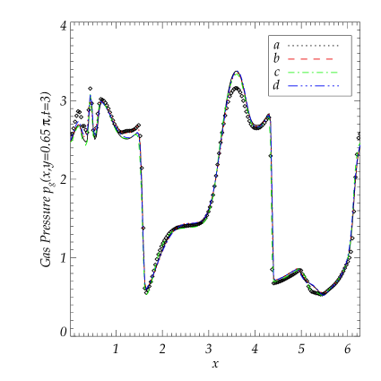
A more detailed comparison is given in Fig. 8, in which the gas pressure distributions along $y=0.625\pi$ at $t=3$ are plotted. At this time, these waves are propagating forward along x axis. There are three obvious differences in these distributions. The most obvious different is the altitude of the hump post first shock – the shock at $x\sim 4.3$. This hump goes through a long term evolving. This difference is caused by particle distributions. Fig. 8 indicates that the BGK solution based scheme is less dissipative than the Maxwellian based scheme. The difference in the fluctuations behind second shock (the one locates at $x\sim 1.6$) is mainly caused by including the Lorentz force effects in the gas evolution. The fluctuations obtained by current scheme is more smooth. The third apparent difference occurring at $x\sim 5.25$ is caused by the implementation of tangential deviations in particle distribution functions.

3.4 Cloud-Shock Interaction[5]

This simplified astrophysical problem describes the disruption of a denser cloud by a magnetosonic shock. The computational domain is $1\times 1$ box solved on a $200\times 200$ mesh. Initially, the rightward-propagating shock locates at $x=0.5$ with a Mach number 10. The left and right states are $(\rho,v_{x},v_{y},v_{z},p_{g},B_{x},B_{y},B_{z})=(3.86859,11.2536,0,0,167.345,0,2.1826182,-2.1826182)$ and $(1,0,0,0,1,0,0.56418985,0.56418985)$, respectively. The circular cloud is centered at $(0.25,0.5)$ with a radius $0.15$ and density $10$. It is in hydrostatic with its surrounding.

Figure 9: The solution of cloud-shock interaction problem at time $t=0.055$. The solution is obtained by 3D BGK MHD code with a very thin third dimension. Density, gas pressure magnetic pressure and kinetic energy are plotted. $\nabla\cdot\vec{B}=0$ is ensured by the field-interpolated constrained transport method. A $200\times 200$ mesh and Curant number $0.7$ are used.

Figure 10: The distributions of various quantities along $y=0.5$ for cloud-shock interaction problem at time $t=0.055$. In the left panel: dots are tot pressure; solid line is gas pressure. In the right panel: dots are magnetic pressure; solid line is density.

This problem is solved by our 3D BGK MHD code with a very thin third dimension. The divergence free condition is ensured by the field-interpolated constrained transport scheme. The Euler scheme is used for time-stepping. If the magnetic resistivity is set $\eta=0$, the calculation easily crashes. Instead of employing the 2nd order TVD Runge-Kutta scheme and the time-consuming projection method ensuing $\nabla\cdot\vec{B}=0$, I increase the resistivity slightly. Numerical experiments show a $\eta=0.008\Delta t$ and $C_{1}=0.2$ are enough to keep the computation stable. The tangential deviations in the distribution function plays a very important role for this case. If we switch off those tangential deviations, the oscillations occur widely and crash the computation. Fig. 10 shows the distributions of various quantities along the middle line $y=0.5$. It is clear that the current scheme can capture shock with $4\sim 7$ cells, even with the artificially enhanced viscosity and resistivity.

3.5 3D Turbulent Magneto-convection

Figure 11: Results of 3D turbulent magneto-convection. Horizontal slices at $z=0.82$. Upper panel: color contours are the vertical component of the velocity; arrows are the horizontal components. Lower panel: color contours are the magnetic strength; arrows are the horizontal components of the magnetic field.

Figure 12: Results of 3D turbulent magneto-convection. Vertical slices at $y=1.67$. Upper panel: color contours are the temperature fluctuation from horizontal mean; arrows are the projection of the velocity on x-z plane. Lower panel: color contours are the magnetic strength; arrows are the projection of the magnetic field on x-z plane.

Figure 13: Results of 3D turbulent magneto-convection. Time history of maximum Mach number. $t=0$ is the initialization time of magentic field. Solid line indicates the property of non-magnetic convection. Dotted line indicates the magnetic convection

The 3D turbulent magneto-convection in the stellar interior is calculated to show the applicability of the current BGK MHD scheme to complicated astrophysical flows. This is one of the most difficult MHD problem in astrophysics. It is essentially a multi- length-scale and time-scale problem, which makes its numerical modeling very time- and memory- consuming. In the deep stellar atmosphere, the convective motions are subsonic. However just beneath the upper radiative zone, there is thin highly superadiabatic layer, where complex waves, including supersonic waves generated. The computation is easily interrupted if the code is not robust, especially, during the thermal relaxation phase of the model.

Here I calculate a 3D sandwich model of stellar convection: one convective layer locates in between two stable layers. The stable layers are radiative. Radiation transfer is treated by diffusion approximation. Under constant gravity, the system is initially in hydrostatic state and vertically stratified. The method to construct the initial stratification can be find in [11]. The middle layer is slightly superadiabatic. The stable layers are subadiabatic. The vertical depth extents $\sim 5.3$ pressure scale heights. The sub-grid scale turbulent behaviors are mimicked by Smagorinsky model[12, 16]. The aspect ratio is $3/1$ (width/depth). The horizontal boundaries are periodic. The upper boundary and lower boundary are impenetrable. All quantities are scaled such that the density, pressure, temperature at the top boundary are unit. The length is scaled by the depth of the computation domain. This initial state will undergo an adjustment, significantly near the vertical boundaries and stable-unstable interface, moderately in the convective region. Finally, the system will be thermally relaxed and approach an dynamic equilibrium state, indicated by the balance between outgoing energy flux through top and input energy flux from bottom.

When the non-magneto convection nearly approaches the relaxed state, I impose a uniform vertical magnetic field to a snapshot of the numerical solutions. Its strength equals the equipartition value near the top. At the top and bottom, the vertical field boundary condition is adopted for the magnetic field, i.e.,

$$B_{x}=B_{y}=0,\frac{\partial B_{z}}{\partial z}=0.$$ (60)

The computation was run on the supercomputer with a 336 threading code parallelized by massage passing interface (MPI) protocol. The computation of non-magnetic convection took $\sim 36$ days, it is still not completely relaxed. The upper boundary can transport around 85 percent of the input energy fluxes. The magneto convection was run for $\sim 7$ days. At the end, 93 percent input fluxes can be transported out from upper lid.

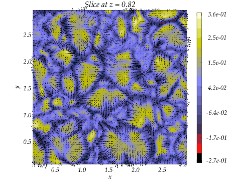
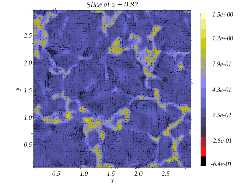
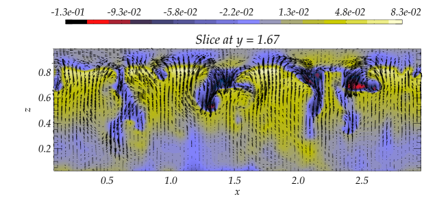
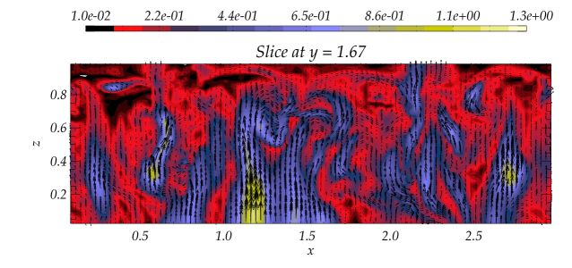
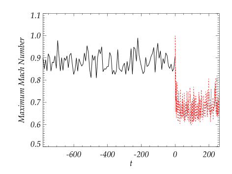
Fig. 11 shows the projections of 3D velocity and magnetic field on a horizontal x-y plane, at $z=0.82$. Upper panel shows the velocity field. Lower panel shows the magnetic field. Color contours are the vertical component. Arrows are horizontal fields. Fig. 12 displays vertical slices of the flows. In upper panel, the 2D velocity field is imposed on the fluctuation of temperature from the horizontal mean. In lower panel, the 2D magnetic field is imposed on the contour of magnetic strength. Fig. 13 shows the time history of the maximum Mach number of the system. The magnetic field suppresses the motion evidently. Before superposing magnetic field, the highest speed motion is nearly supersonic.

4 Discussion

The current scheme can be regarded as a hybrid method, a combination of BGK-NS solver and flux splitting scheme. Without introducing parameter-controlled equilibrium state, the treatment of the magnetic part of fluxes is similar to the FVS scheme. Unlike the FVS scheme and the gas-kinetic MHD method developed by Xu[19], where the Maxwellian distribution is used, the current method splits the solution of BGK equation. The collision mechanism is already included in the split distribution. Physically, the current scheme is supposed to be better. However, numerical tests show that the improvement is not very great. For some cases, it is dispersive.

For non-magnetic flows, the tangential deviations from equilibrium state in particle distribution function play a role in improving the accuracy of the scheme. After implementing the magnetic field, the effects become case-dependent. The effects of tangential terms can be thought as reducing the numerical dissipation. For some cases, eg., 2D Orzang-Tang vortex, this kind of reduction seems too much, even with a 2nd order TVD Runge-Kutta time marching scheme. To get around with this kind of situation, it is better to switch off these tangential deviations terms in particle distribution functions.

As stated before, the particle solution from solving BGK equation can be split into three parts, i.e., $[\cdots]g_{0}$, split parts $[\cdots]g_{0}^{l}$ and $[\cdots]g_{0}^{r}$, just like Maxwellian based scheme, i.e., $(1-\alpha)g_{0}$, $\alpha g_{0}^{l}$ and $\alpha g_{0}^{r}$. The adjustable parameter is replaced by complicated coefficients from solving BGK equation. It sounds more physical. Numerical tests again show that this kind of consideration would make a very dispersive scheme. This is because in Maxwellian based scheme, the particle collisions are controlled by an universal constant $\alpha$, so the numerical dissipation from MUSCL-type reconstruction is added in whole computational domain. In the BGK scheme, the numerical dissipation only become large near the region where the particle distribution deviates from equilibrium state significantly. More specifically, the equilibrium term and non-equilibrium terms from (26) can be expressed as $[1+e^{-t/\tau}+\cdots]g_{0}$, split parts $[e^{-t/\tau}(\cdots)]g_{0}^{l}$ and $[e^{-t/\tau}(\cdots)]g_{0}^{r}$. $e^{-t/\tau}$ is a very small number, because usually we have $\tau\lesssim t/10$, which means the split parts can be ignored. $\tau$ only becomes comparable to $t$ near the high non-equilibrium region. This is reason why BGK is a very robust and accurate scheme for non-magnetic shock wave problems. For magnetic flows, the equilibrium part $[1+e^{-t/\tau}+\cdots]g_{0}$ needs to be split also to include enough dissipation to smooth the dispersion.

Fig. 3 shows clearly that the dispersion occurs near the front of fast wave and propagates backward. Microscopically, transport of flow properties can be regarded as a consequence of particle motions and the amount of flux is proportional to the number of involved particles. This is not true for the magnetic field, even those advective terms. This is because the unlike charge or mass, there is no specific amount magnetic is carried by each particle. If we treat the non-magnetic part by a second order time scheme, while the magnetic field by a first oder time scheme. Although, the magnetic terms are weighted by second order particle distributions, the difference of time accuracy of these two parts is still big. The truncation errors propagate at different speed, which amplifies the numerical dispersion. A second-order TVD Runge-Kutta scheme can smear out these oscillations.

The second-order TVD time scheme usually catches a sloping shock front. A way to improve this is to design a very smart parameter $\alpha$ that can introduce numerical dissipation both near the shock and the fast waves. In [15] $\alpha$ is adaptive according to the discontinuity in magnetic pressure. A more consistent way to construct a gas-kinetic theory based MHD scheme is to considers separately the distribution of charged particle (electrons and ions) and electrically neutral particle. Model the long distance interactions between charged particles and then integrate the electric field and magnetic properties from the motion of these charged particles. In such case, the EOS play a very important role, since it determines the number of charged particles. Obviously, this is a very complicated method. A more detailed discussion is beyond the scope of current study.

The gas-kinetic MHD scheme developed in [14] is an efficient method. For the 2D Orzang-Tang vortex problem tested in this paper, it can be two times faster than the current scheme (with $\sim 0.47$ time-consuming). However, in application to astrophysical problems, a lot of things, such as radiation transfer, turbulent modeling, moving mesh generating, need to be implemented. The hydrodynamics part of the code is not the major agent consuming the computation time. Sometimes, even the ensuring divergence free constraint takes a lot time. For instance, for the 2D tests in this paper, a Possion equation is solved to ensue $\nabla\cdot\vec{B}=0$. This involves an implicit solver. The time-consuming of an implicit solver is generally not linearly proportional to the grid points. The MHD code based on current scheme is capable of calculating the complicated HD problem without extra efforts. At the same time, it is also a high order MHD solver.

5 Conclusion

This paper presents a feasible way to extend the multidimensional gas-kinetic BGK scheme to MHD problems. The non-magnetic part is solved by the BGK scheme modified due to magnetic field. While the magnetic part is calculated by gas-kinetic flux splitting based on a solution of BGK equations. Besides keeping high robustness and accuracy for HD problem, the current scheme is also a high order MHD solver. The effects of tangential deviations and Lorentz force in particle distribution are numerically studied. Although case-dependent, it is better to include them for most of the cases. Numerical tests also show that compared to the Maxwellian based gas-kinetic flux splitting scheme, the current scheme is more stable for 1D problems and less dissipative for multidimensional problems. The 3D turbulent magneto-convection test indicates the applicability of current scheme to complicated astrophysical flows. The gas-kinetic theory based flux splitting methods for MHD problems can be improved by designing a more smart parameter $\alpha$. A full gas-kinetic scheme for MHD needs to consider the complicated physical processes, such as particle charging and long distance Coulomb force.

6 Acknowledgments

The computations of 3D turbulent magneto-convection were tested and performed on Eövös University’s 416-core, 3.7 Tflop HPC cluster Atlasz and on the supercomputing network of the NIIF Hungarian National Supercomputing Center (project ID: 1117 fragment). The current research was supported by the European Commission’s 6th Framework Programme (SOLAIRE Network, MTRN-CT-2006-035484).

References

- Bhatnagar et al. [1954] P.L. Bhatnagar, E.P. Gross, M. Krook, A model for collision processes in gases. i. small amplitude processes in charged and neutral one-component systems, Phys. Rev. 94 (1954) 511–525.
- Brio and Wu [1988] M. Brio, C.C. Wu, An upwind differencing scheme for the equations of ideal magnetohydrodynamics, Journal of Computational Physics 75 (1988) 400 – 422.
- Colella and Woodward [1984] P. Colella, P.R. Woodward, The piecewise parabolic method (ppm) for gas-dynamical simulations, Journal of Computational Physics 54 (1984) 174 – 201.
- Dai and Woodward [1994] W. Dai, P.R. Woodward, Extension of the piecewise parabolic method to multidimensional ideal magnetohydrodynamics, Journal of Computational Physics 115 (1994) 485 – 514.
- Dai and Woodward [1998] W. Dai, P.R. Woodward, A simple finite difference scheme for multidimensional magnetohydrodynamical equations, Journal of Computational Physics 142 (1998) 331 – 369.
- Harten [1983] A. Harten, High resolution schemes for hyperbolic conservation laws, Journal of Computational Physics 49 (1983) 357 – 393.
- Orszag and Tang [1979] S.A. Orszag, C.M. Tang, Small-scale structure of two-dimensional magnetohydrodynamic turbulence, Journal of Fluid Mechanics 90 (1979) 129–143.
- Ryu and Jones [1995] D. Ryu, T.W. Jones, Numerical magetohydrodynamics in astrophysics: Algorithm and tests for one-dimensional flow‘, Apj 442 (1995) 228–258.
- Ryu et al. [1995] D. Ryu, T.W. Jones, A. Frank, Numerical Magnetohydrodynamics in Astrophysics: Algorithm and Tests for Multidimensional Flow, Apj 452 (1995) 785–+.
- Shu [1988] C.W. Shu, Total-Variation-Diminishing Time Discretizations, SIAM J. Sci. and Stat. Comput. 9 (1988) 1073–1084.
- Singh et al. [1995] H.P. Singh, I.W. Roxburgh, K.L. Chan, Three-dimensional simulation of penetrative convection: penetration below a convection zone., AA 295 (1995) 703–+.
- Smagorinsky [1963] J. Smagorinsky, General Circulation Experiments with the Primitive Equations, Monthly Weather Review 91 (1963) 99–+.
- Steger and Warming [1981] J.L. Steger, R.F. Warming, Flux vector splitting of the inviscid gasdynamic equations with application to finite-difference methods, Journal of Computational Physics 40 (1981) 263 – 293.
- Tang and Xu [2000] H.Z. Tang, K. Xu, A high-order gas-kinetic method for multidimensional ideal magnetohydrodynamics, Journal of Computational Physics 165 (2000) 69 – 88.
- Tang et al. [2010] H.Z. Tang, K. Xu, C. Cai, Gas-kinetic bgk scheme for three dimensional magnetohydrodynamics, Numer. Math. Theor. Meth. Appl. 3 (2010) 387 – 404.
- Tian et al. [2009] C. Tian, L. Deng, K. Chan, D. Xiong, Efficient turbulent compressible convection in the deep stellar atmosphere, Research in Astronomy and Astrophysics 9 (2009) 102–114.
- Tian et al. [2007] C.L. Tian, K. Xu, K.L. Chan, L.C. Deng, A three-dimensional multidimensional gas-kinetic scheme for the Navier Stokes equations under gravitational fields, Journal of Computational Physics 226 (2007) 2003–2027.
- Tóth [2000] G. Tóth, The constraint in shock-capturing magnetohydrodynamics codes, Journal of Computational Physics 161 (2000) 605 – 652.
- Xu [1999] K. Xu, Gas-kinetic theory-based flux splitting method for ideal magnetohydrodynamics, Journal of Computational Physics 153 (1999) 334 – 352.
- Xu [2001] K. Xu, A gas-kinetic bgk scheme for the navier-stokes equations and its connection with artificial dissipation and godunov method, Journal of Computational Physics 171 (2001) 289 – 335.
- Xu and Prendergast [1994] K. Xu, K.H. Prendergast, Numerical navier-stokes solutions from gas kinetic theory, Journal of Computational Physics 114 (1994) 9 – 17.
- Zachary et al. [1994] A.L. Zachary, A. Malagoli, P. Colella, A higher-order godunov method for multidimensional ideal magnetohydrodynamics, SIAM Journal on Scientific Computing 15 (1994) 263–284.