The perfect integrator driven by Poisson input and its approximation in the diffusion limit

Abstract

In this note we consider the perfect integrator driven by Poisson process input. We derive its equilibrium and response properties and contrast them to the approximations obtained by applying the diffusion approximation. In particular, the probability density in the vicinity of the threshold differs, which leads to altered response properties of the system in equilibrium.

Moritz Helias¹, Moritz Deger², Stefan Rotter^2,3, and Markus Diesmann^1,4,5

¹Computational Neurophysics, RIKEN Brain Science Institute, Wako City, Japan
²Bernstein Center Freiburg, Germany
³Computational Neuroscience, Faculty of Biology, Albert-Ludwig University, Freiburg, Germany
⁴Institute of Neuroscience and Medicine, Computational and Systems Neuroscience (INM-6), Research Center Juelich, Juelich, Germany
⁵Brain and Neural Systems Team, Computational Science Research Program, RIKEN, Wako City, Japan

Stationary solution of perfect integrator with excitation

The membrane potential $V$ of the perfect integrator (Tuckwell, 1988) evolves according to the stochastic differential equation

$$\frac{dV}{dt} =w\sum_{i}\delta(t-t_{i}),$$

where $t_{i}$ are random time points of synaptic impulses events generated by a Poisson process with rate $\lambda$ and $w$ is the magnitude is the voltage change caused by an incoming event. If $V$ reaches the threshold $V_{\theta}$ the neuron emits an action potential. After the threshold crossing, the voltage is reset to $V\leftarrow V-(V_{\theta}-V_{r})$. This reset preserves the overshoot above threshold and places the system above the reset value by this amount. Biophysically the reset is motivated by considering each $\delta$-impulse as the limit of a current extended in time. If $V$ crosses $V_{\theta}$ within such a pulse, after the reset to $V_{r}$ the remainder of the pulse’s charge causes a depolarization starting from $V_{r}$. We consider a population of identical neurons and assume a uniformly distributed membrane voltage between reset and threshold initially. In what follows we apply the formalism outlined in Helias et al. (2010). The first and second infinitesimal moment (Ricciardi et al., 1999) of the diffusion approximation are

$$A_{1} =\lambda w\stackrel{{\scriptstyle\mathrm{def}}}{{=}}\mu$$

$$A_{2} =\lambda w^{2}\stackrel{{\scriptstyle\mathrm{def}}}{{=}}\sigma^{2}.$$

The corresponding neuron driven by Gaussian white noise hence obeys the stochastic differential equation

$$\frac{dV}{dt}=\mu+\sigma\xi(t),$$

with the zero mean Gaussian white noise $\xi$, $\langle\xi(t)\xi(t+s)\rangle_{t}=\delta(s)$. The probability flux operator is

$$S=\mu-\frac{\sigma^{2}}{2}\frac{\partial}{\partial V}.$$

We renormalize the stationary probability density $p(V)$ by the as yet unknown flux $\nu$ as $q(V)=\frac{1}{\nu}p(V)$ so that the equilibrium density fulfills the stationary Fokker-Planck equation

$$Sq(V)=1_{V_{r}<V<V_{\theta}}.$$ (1)

Here $1_{\mathrm{expr.}}$ equals $1$ if $\mathrm{expr.}$ is true, and $0$ else. The homogeneous solution of (1) is

$$q_{h}(V)=e^{\frac{2\mu}{\sigma^{2}}V},$$

the particular solution which vanishes at $V=V_{\theta}$ for $V_{r}<V<V_{\theta}$ is

$$q_{p}(V) =-\frac{2}{\sigma^{2}}e^{\frac{2\mu}{\sigma^{2}}V}\int_{V_{\theta}}^{V}e^{-\frac{2\mu}{\sigma^{2}}u}\;du$$

$$=\frac{1}{\mu}\left(1-e^{\frac{2\mu}{\sigma^{2}}(V-V_{\theta})}\right).$$

We first consider the case of Gaussian white noise input of mean $\mu$ and variance $\sigma$. A finite probability flux in this case requires $q(V_{\theta})=0$ at threshold. We hence obtain the full solution that is continuous at reset as

$$q(V)=\frac{1}{\mu}\begin{cases}1-e^{\frac{2\mu}{\sigma^{2}}(V-V_{\theta})}&\text{for }V_{r}<V<V_{\theta}\\ e^{\frac{2\mu}{\sigma^{2}}V}\left(e^{-\frac{2\mu}{\sigma^{2}}V_{r}}-e^{-\frac{2\mu}{\sigma^{2}}V_{\theta}}\right)&\text{for }-\infty<V<V_{r}.\end{cases}$$

The normalization $1=\int p(V)\;dV=\nu\int q(V)\;dV$ determines the firing rate as

$$\nu=\frac{\mu}{V_{\theta}-V_{r}}=\frac{\lambda w}{V_{\theta}-V_{r}},$$ (2)

With $\mu/\sigma^{2}=1/w$ the density is

$$p(V)=\frac{1}{V_{\theta}-V_{r}}\begin{cases}1-e^{\frac{2}{w}(V-V_{\theta})}&\text{for }V_{r}<V<V_{\theta}\\ e^{\frac{2}{w}V}\left(e^{-\frac{2}{w}V_{r}}-e^{-\frac{2}{w}V_{\theta}}\right)&\text{for }-\infty<V<V_{r}.\end{cases}$$ (3)

We next take into account the finite synaptic jumps to obtain a modified boundary condition (Helias et al., 2010) at the firing threshold. For $V_{r}<V<V_{\theta}$ the solution of (1) implies a recurrence relation between higher derivatives, such that the $n$-th derivative $q^{(n)}$ can be expressed in terms of the function value itself as

$$q^{\prime} =\frac{2\mu}{\sigma^{2}}q-\frac{2}{\sigma^{2}}$$

$$q^{\prime\prime} =\frac{2\mu}{\sigma^{2}}q^{\prime}=\frac{2\mu}{\sigma^{2}}\left(\frac{2\mu}{\sigma^{2}}q-\frac{2}{\sigma^{2}}\right)=\left(\frac{2\mu}{\sigma^{2}}\right)^{2}q-\mu\left(\frac{2}{\sigma^{2}}\right)$$

$$q^{(n)} =\underbrace{\left(\frac{2\mu}{\sigma^{2}}\right)^{n}}_{d_{n}}q\underbrace{-\frac{2}{\sigma^{2}}\left(\frac{2\mu}{\sigma^{2}}\right)^{n-1}}_{c_{n}},$$

with $d_{0}=1$ and $c_{0}=0$ for completeness. Applying equation (8) of Helias et al. (2010) allows to determine the boundary value at threshold as

$$q(V_{\theta}) =\frac{1+\lambda\sum_{n=0}^{\infty}\frac{1}{(n+1)!}c_{n}(-w)^{n+1}}{-\lambda\sum_{n=0}^{\infty}d_{n}(-w)^{n+1}}$$

$$=\frac{1+\lambda\left(-\frac{1}{\sigma^{2}}w^{2}+\frac{1}{6}(-\frac{4\mu}{\sigma^{4}})(-w)^{3}\right)}{-\lambda\left(-w+\frac{\mu}{\sigma^{2}}w^{2}+\frac{1}{6}(2\frac{\mu}{\sigma^{2}})^{2}(-w^{3})\right)}$$

$$=\frac{\frac{4}{6}\frac{\mu}{\sigma^{4}}w^{3}}{\frac{4}{6}\frac{\mu^{2}}{\sigma^{4}}w^{3}}=\frac{1}{\mu}.$$

In the case of finite jumps, the region below reset will never be entered, hence $q(V)=0$ for $V<V_{r}$. In order for the solution to fulfill the boundary value at threshold the homogeneous solution $q_{h}(V)=\mu^{-1}e^{2\mu(V-V_{\theta})/\sigma^{2}}$needs to be added to the particular solution $q_{p}$, so the complete stationary density is

$$q(V)=\begin{cases}\frac{1}{\mu}&\text{for }V_{r}<V<V_{\theta}\\ 0&\text{for }-\infty<V<V_{r}.\end{cases}$$

The normalization therefore yields the same firing rate as in the case of Gaussian white noise

$$\nu=\frac{\mu}{V_{\theta}-V_{r}}=\frac{\lambda w}{V_{\theta}-V_{r}}.$$ (4)

This expression agrees with the intuitive expectation, because $\frac{V_{\theta}-V_{r}}{w}$ input impulses are needed to cause an output spike. Using this normalization, the density is

$$p(V)=\begin{cases}\frac{1}{V_{\theta}-V_{r}}&\text{for }V_{r}<V<V_{\theta}\\ 0&\text{for }-\infty<V<V_{r}.\end{cases}$$ (5)

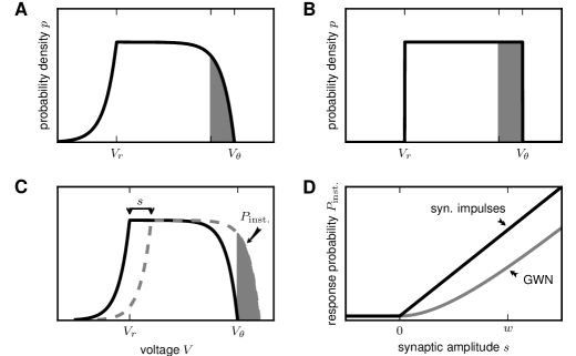
Figure 1: Equilibrium density and response shaped by background. (A) Probability density of voltage $V$ of a perfect integrator driven by Gaussian white noise (3). (B) Probability density of a perfect integrator driven with excitatory synaptic impulses of finite size $w$ causing the same drift and fluctuations as in A (5). The density near threshold most strongly differs on the scale of the synaptic amplitude $w$ (gray shaded region). (C) An additional excitatory impulse of amplitude $s$ shifts the density (shown for Gaussian white noise background input as in A), so that the gray shaded area exceeds the threshold. (D) The probability $P_{\text{inst.}}$ to respond with an action potential corresponds to the area of density above threshold in C; it depends on the shape of the density near threshold (black: background of synaptic impulses of size $w$ (7); gray: Gaussian white noise background (6)). Parameters: $w=3\>\mathrm{mV}$, $V_{r}=0$, $V_{\theta}=15\>\mathrm{mV}$ and $\lambda=200\;\frac{1}{s}$.

The solutions for both cases are illustrated in Fig. 1A,B.

Instantaneous and time dependent response

The probability $P_{\text{inst.}}(s)$ that a neuron in the population instantaneously emits an action potential in response to a single synaptic input of postsynaptic amplitude $s$ equals the probability mass $P_{\text{inst.}}(s)=\int_{V_{\theta}-s}^{V_{\theta}}p(V)\;dV$ crossing the threshold (shaded region in Fig. 1C). In the the case of Gaussian white noise with (3)

$$P_{\text{inst.}}(s) =\int_{V_{\theta}-s}^{V_{\theta}}p(V)\;dV$$

$$=1_{s>0}\left(\frac{s}{V_{\theta}-V_{r}}-\frac{w/2}{V_{\theta}-V_{r}}\left(1-e^{-\frac{2s}{w}}\right)\right)$$

$$=1_{s>0}\frac{1}{V_{\theta}-V_{r}}\left(s+\frac{w}{2}\left(e^{-\frac{2s}{w}}-1\right)\right).$$ (6)

This expression grows quadratically like $P_{\text{inst.}}(s)\simeq 1_{s>0}\frac{1}{V_{\theta}-V_{r}}\frac{s^{2}}{w}$ for small synaptic amplitudes $s$ as shown in Fig. 1D. In the case of finite synaptic jumps using (5) we get

$$P_{\text{inst.}}(s)=1_{s>0}\frac{s}{V_{\theta}-V_{r}}.$$ (7)

The response grows linear in the amplitude $s$ of the additional perturbing spike (Fig. 1D). A linear approximation of the integral response can be obtained using the slope of the equilibrium rate (4) with respect to $\mu$ as

$$P_{\text{int.}}(s)=\int_{0}^{\infty}\nu(t)-\nu\;dt=s\frac{\partial\nu}{\partial\mu}=\frac{s}{V_{\theta}-V_{r}}.$$

For positive $s$ this expression equals the integral instantaneous response (7) so the complete response is instantaneous in this case. For $s<0$ we only consider the special case of a synaptic inhibitory pulse with the same magnitude $s=-w$ as the excitatory background pulses, so the density is shifted away from threshold by $w$ and the firing rate goes to $0$. The density reaches threshold again if at least one excitatory pulse has arrived, which occurs within time $t$ with probability $P_{k\geq 1}=1-e^{-\lambda t}$. Given the excitatory event, the hazard rate of the neuron is $\frac{\lambda w}{V_{\theta}-V_{r}}$, so the time dependent response is

$$\nu(t)=(1-1_{t>0}e^{-\lambda t})\frac{\lambda w}{V_{\theta}-V_{r}}.$$ (8)

The density after the inhibitory event therefore is a superposition of the shifted density and the equilibrium density with the relative weighting given by the probabilities $1-P_{k\geq 1}$ and $P_{k\geq 1}$, respectively

$$p(V,t) =\frac{1}{V_{\theta}-V_{r}}\begin{cases}1_{t>0}e^{-\lambda t}&\text{for }V_{r}-w<V<V_{\theta}-w\\ 1-1_{t>0}e^{-\lambda t}&\text{for }V_{r}<V<V_{\theta}.\end{cases}$$ (9)

The time evolution of the density following an excitatory and following an inhibitory impulse at $t=0$ is shown in Fig. 2 A and B, respectively.

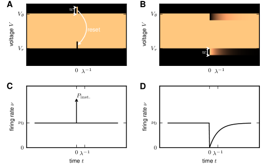
Figure 2: Asymmetry of response. (A) An additional excitatory impulse of amplitude $w$ shifts the probability density upwards such that a small part of the density exceeds the threshold. This leads to an instantaneous spiking response, visible as a $\delta$-shaped deflection in firing rate $\nu$ (visualized by bars of finite width in A and C). The reset of the membrane voltage to $V_{r}$ after the spike moves the exceeding density down, so the density immediately equals the state before the impulse. (B) An additional inhibitory impulse of amplitude $-w$ deflects the density downwards (9). It does not cause a response concentrated at the time of the impulse (D). Instead, the firing rate $\nu$ instantaneously drops and exponentially reapproaches its equilibrium value $\nu_{0}$ (8) as the density gradually relaxes to its steady state on the time scale $1/\lambda$, where $\lambda$ is the rate of synaptic background impulses.

The integrated response probability

$$P_{\text{int.}}(-w) =\int_{0}^{\infty}\nu(t)-\nu\;dt$$

$$=-\frac{\lambda w}{V_{\theta}-V_{r}}\int_{0}^{\infty}e^{-\lambda t}\;dt$$

$$=-\frac{w}{V_{\theta}-V_{r}},$$

is the same as for an excitatory spike and coincides with the linear approximation.

Stochastic resonance

In order to observe stochastic resonance, the fluctuation in the input to the perfect integrator must be varied. We therefore consider a zero mean Gaussian white noise input current $\sigma\xi(t)$. Adding a constant restoring force $\mu(V)=-\mu_{0}\mathrm{sign}(V-V_{r})$, $\mu_{0}>0$ assures that the voltage trajectories do not diverge to $-\infty$ and approach $V_{r}$ in absence of synaptic input. The homogeneous solution of the stationary Fokker-Planck equation analog to (1) therefore is $q_{h}(V)=e^{-\frac{2\mu_{0}}{\sigma^{2}}|V-V_{r}|}$. The particular solution for $V>V_{r}$ that fulfills the boundary condition $q(V_{\theta})=0$ is found by variation of constants as

$$q_{p}(V)=\frac{1}{\mu_{0}}\left(e^{-\frac{2\mu_{0}}{\sigma^{2}}(V-V_{\theta})}-1\right),$$

so the complete solution follows as

$$q(V)=\frac{1}{\mu_{0}}\begin{cases}\left(e^{-\frac{2\mu_{0}}{\sigma^{2}}(V-V_{\theta})}-1\right)&\text{for }V_{r}<V<V_{\theta}\\ \left(e^{-\frac{2\mu_{0}}{\sigma^{2}}(V_{r}-V_{\theta})}-1\right)e^{\frac{2\mu_{0}}{\sigma^{2}}(V-V_{r})}&\text{for }-\infty<V<V_{r}.\end{cases}$$

Normalization again yields the equilibrium rate $\nu$

$$1 =\nu\int q(V)\;dV$$

$$\nu =\frac{\mu_{0}}{\frac{\sigma^{2}}{\mu_{0}}\left(e^{\frac{2\mu_{0}}{\sigma^{2}}(V_{\theta}-V_{r})}-1\right)+V_{r}-V_{\theta}},$$

and the normalized density is

$$p(V)=\frac{\nu}{\mu_{0}}\begin{cases}e^{\frac{2\mu_{0}}{\sigma^{2}}(V_{\theta}-V)}-1&\text{for }V_{r}<V<V_{\theta}\\ \left(e^{\frac{2\mu_{0}}{\sigma^{2}}(V_{\theta}-V_{r})}-1\right)e^{\frac{2\mu_{0}}{\sigma^{2}}(V-V_{r})}&\text{for }-\infty<V<V_{r}.\end{cases}$$ (10)

Fig. 3B visualizes the density for three different fluctuation amplitudes $\sigma$. In the limit of large $\sigma^{2}\gg\mu_{0}$ the density decreases proportional to $1/\sigma^{2}$ between reset and threshold and falls off linearly towards threshold

$$p(V)\simeq\begin{cases}\frac{2\mu_{0}}{\sigma^{2}}\frac{V_{\theta}-V}{V_{\theta}-V_{r}}&\text{for }V_{r}<V<V_{\theta}\\ \frac{2\mu_{0}}{\sigma^{2}}\left(1+\frac{2\mu_{0}}{\sigma^{2}}(V-V_{r})\right)&\text{for }-\infty<V<V_{r}.\end{cases}$$

The red curve in Fig. 3B shows the tendency of such a linear decay towards threshold. The instantaneous response exhibits stochastic resonance, because the integrated voltage density near threshold assumes a maximum at a particular noise level $\sigma$. This can already be judged from the zoom-in near threshold in Fig. 3C. Formally, the response to an incoming impulse of amplitude $s$ is

$$P_{\text{inst.}}(s) =\int_{V_{\theta}-s}^{V_{\theta}}p(V)\;dV=\frac{1}{\frac{\sigma^{2}}{\mu_{0}}\left(e^{\frac{2\mu_{0}}{\sigma^{2}}(V_{\theta}-V_{r})}-1\right)+V_{r}-V_{\theta}}\left(-\frac{\sigma^{2}}{2\mu_{0}}\left(1-e^{\frac{2\mu_{0}}{\sigma^{2}}s}\right)-s\right)$$

$$\stackrel{{\scriptstyle s\ll\sigma}}{{\simeq}}\frac{1}{\frac{\sigma^{2}}{\mu_{0}}\left(e^{\frac{2\mu_{0}}{\sigma^{2}}(V_{\theta}-V_{r})}-1\right)+V_{r}-V_{\theta}}\;\frac{\mu_{0}}{\sigma^{2}}s^{2}$$

$$=\frac{s^{2}}{\frac{\sigma^{4}}{\mu_{0}^{2}}\left(e^{\frac{2\mu_{0}}{\sigma^{2}}(V_{\theta}-V_{r})}-1\right)+\frac{\sigma^{2}}{\mu_{0}}\left(V_{r}-V_{\theta}\right)}.$$ (11)

The dependence on the noise is graphed in Fig. 3D.

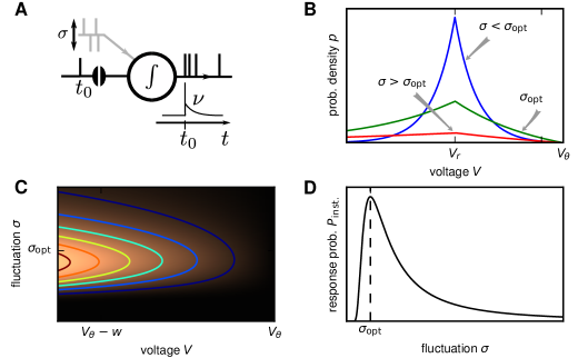
Figure 3: Stochastic resonance. (A) A model neuron receives balanced excitatory and inhibitory background input (gray spikes). The probability of a particular synaptic impulse (black vertical bar at $t_{0}$) to elicit an immediate response by depends on the amplitude $\sigma$ of the fluctuations caused by the other synaptic afferents. (B) The spread of the probability density of voltage depends on the amplitude $\sigma$ of the fluctuations caused by all synaptic afferents (10). At low fluctuations ($\sigma<\sigma_{\text{opt}}$) it is unlikely to find the voltage near threshold, the density there is negligible (blue: $\sigma=5.5\>\mathrm{mV}$). At intermediate fluctuations ($\sigma_{\text{opt}}$), the probability of finding the density below threshold is elevated (green: $\sigma=11\>\mathrm{mV}$). Increasing the fluctuations beyond this point ($\sigma>\sigma_{\text{opt}}$) spreads out the density to negative voltages, effectively depleting the range near threshold (red: $\sigma=16.5\>\mathrm{mV}$). (C) Zoom-in of the probability density near threshold (luminance coded with iso-density lines) over voltage $V$ (horizontal axis) as a function of the magnitude of fluctuations $\sigma$ (vertical axis). At the optimal level $\sigma_{\text{opt}}$, the density near threshold becomes maximal. (D) The voltage integral of this density determines the probability of eliciting a spike (11) and has a single maximum at $\sigma_{\text{opt}}$. Further parameters are $V_{r}=0$, $V_{\theta}=15\>\mathrm{mV}$, $\mu_{0}=5.0\>\mathrm{mV}/s$.

References

Helias et al. [2010]
M. Helias, M. Deger, S. Rotter, and M. Diesmann.
Instantaneous non-linear processing by pulse-coupled threshold units.
PLoS Comput Biol, 6(9):e1000929, 2010.
doi:10.1371/journal.pcbi.1000929.
Ricciardi et al. [1999]
L. M. Ricciardi, A. Di Crescenzo, V. Giorno, and A. G. Nobile.
An outline of theoretical and algorithmic approaches to first passage
time problems with applications to biological modeling.
MathJaponica, 50(2):247–322, 1999.
Tuckwell [1988]
Henry C. Tuckwell.
Introduction to Theoretical Neurobiology, volume 1.
Cambridge University Press, Cambridge, 1988.
ISBN 0-521-35096-4.