QED confronts the radius of the proton

Abstract

Recent results on muonic hydrogen [1] and the ones compiled by CODATA on ordinary hydrogen and $ep$-scattering [2] are $5\sigma$ away from each other. Two reasons justify a further look at this subject: 1) One of the approximations used in [1] is not valid for muonic hydrogen. This amounts to a shift of the proton’s radius by $\sim 3$ of the standard deviations of [1], in the “right” direction of data-reconciliation. In field-theory terms, the error is a mismatch of renormalization scales. Once corrected, the proton radius “runs”, much as the QCD coupling “constant” does. 2) The result of [1] requires a choice of the “third Zemach moment”. Its published independent determination is based on an analysis with a $p$-value –the probability of obtaining data with equal or lesser agreement with the adopted (fit form-factor) hypothesis– of $3.92\times 10^{-12}$. In this sense, this quantity is not empirically known. Its value would regulate the level of “tension” between muonic- and ordinary-hydrogen results, currently at most $\sim 4\sigma$. There is no tension between the results of [1] and the proton radius determined with help of the analyticity of its form factors.

I Introduction

The results of a measurement by Pohl et al. Pohl of the Lamb shift in muonic hydrogen and those compiled by CODATA on ordinary hydrogen and $ep$-scattering CODATA are $\sim 5\,\sigma$ away from each other. The authors of Pohl conclude “Our result implies that either the Rydberg constant has to be shifted by 2110 kHz/c (4.9 standard deviations), or the calculations of the QED effects in atomic hydrogen or muonic hydrogen atoms are insufficient.” I discuss why the second option is part of the resolution of the apparent conundrum, but not all of it.

It is intrepid rpADR to use a model of the proton –in Pohl , a dipole form-factor– to challenge very well established physics –such as QED Pohl ; Flowers . But this is not the only bone of contention:

One of the approximations used in the theory of ordinary or muonic hydrogen involves the lepton’s wave function at the origin. The approximation is sufficiently good for the former atom, but not the latter. The required correction can be rephrased by having an $r_{p}$ that runs, in the same sense as $\alpha_{s}$ –the fine structure constant of QCD– does. The modification results in a $\sim 3\,\sigma(\mu H)$ shift of the extracted central value of $r_{p}$, in the direction of reducing the “tension” between experimental results. This correction depends on the model of the proton’s charge distribution, but the model-dependence is a small correction to a moderate correction. These issues are discussed in detail in Sections III and IV.

The current way to extract $r_{p}$ from $ep$ scattering data involves an extrapolation to a momentum transfer ${\mathbf{q}^{2}}=0$, the point from which $\langle r_{p}^{2}\rangle$ is inferred. This extrapolation covers a two-orders of magnitude larger hiatus than the one relevant to muonic hydrogen; the model-dependence is correspondingly larger. The extrapolated object is a form-factor fit to data gathered above $|{\mathbf{q}}^{2}|={\cal{O}}(m_{\pi}^{2})$, a domain where there is still “structure”, relative to, e.g. a dipole form factor Mainz .

The extraction of $r_{p}$ from $ep$ data has severe statistical problems, mentioned in the abstract and discussed in Section V. One way to reappraise this issue is to take new, very precise data Mainz , see also Section V. The difficulties associated with these analyses are shared by the measurement of the other relevant quantity: the “third Zemach moment”, as discussed in Section VI and VII.

Sections VIII is a discussion of the experimental and theoretical results. Section IX contains my conclusions.

II The issue

Former precise measurements of $r_{p}$ had two origins. One is mainly based on the theory HTheory and observations Hexps of hydrogen. The result, compiled in CODATA CODATA , is

$$\sqrt{\langle r_{p}^{2}\rangle}\rm(CODATA)=0.8768\pm 0.0069\;\rm fm.$$ (1)

The second type of measurement is based on the theory and observations Sick ; Sick2 of very low-energy electron-proton scattering. An analysis of the world data as of a few years ago yielded Sick :

$$\sqrt{\langle r_{p}^{2}\rangle}(ep)=0.895\pm 0.018\;\rm fm$$ (2)

A recent $ep$-scattering experiment Mainz results in:

$$\sqrt{\langle r_{p}^{2}\rangle}\rm(A1)=0.879(5)_{stat}(4)_{syst}(2)_{model}(4)_{group}\;\rm fm,$$ (3)

whose various subindices will be clarified anon.

The proton’s charge distribution, $\rho_{p}(r)$, is related to the non-relativistic limit of the electric form-factor, $G_{E}$, by the Fourier transformation

$$G_{E}(-{\mathbf{q}}^{2})=\int d^{3}r\,\rho_{p}({\mathbf{r}})\,e^{-i\,\vec{q}\,\vec{r}}\simeq 1-{{\mathbf{q}}^{2}\over 6}\,{\langle r_{p}^{2}\rangle}+\,...\,,$$ (4)

which also serves to define ${\langle r_{p}^{2}\rangle}$ in proportion to the ${\mathbf{q}}^{2}$-derivative of the form factor at ${\mathbf{q}}^{2}=0$.

The most precise relevant measurement to date is that of the $\rm 2P_{3/2}^{F=2}\to 2S_{1/2}^{F=1}$ Lamb shift in the $\mu p$ atom, Pohl :

$$L_{\rm exp}=206.2949\pm 0.0032\;\rm meV.$$ (5)

In meV units for energy and fermi units for the radii, the predicted value LymanTH is of the form

$$L^{\rm th}\left[\langle r_{p}^{2}\rangle,\langle r_{p}^{3}\rangle_{(2)}\right] =$$

$$209.9779(49) - 5.2262\,\langle r_{p}^{2}\rangle+0.00913\,\langle r_{p}^{3}\rangle_{(2)}$$ (6)

The first two coefficients are best estimates of many contributions while the third stems from the $n=2$ value of an addend FriarSick ; HTheory

$$\Delta E_{3}(n,l)={\alpha^{5}\over 3\,n^{3}}\,m_{r}^{4}\,\delta_{l0}\,\langle r_{p}^{3}\rangle_{(2)},$$ (7)

proportional to the third Zemach moment

$$\langle r_{p}^{3}\rangle_{(2)}\equiv\int d^{3}r_{1}d^{3}r_{2}\,\rho(r_{1})\rho(r_{2})|{\mathbf{r}}_{1}-{\mathbf{r}}_{2}|^{3}$$ (8)

For a specific model of $\rho_{p}(r)$ or its corresponding $G_{E}(-{\mathbf{q}}^{2})$, the two $r$-moments in Eq. (6) are related. For instance, for a dipole form factor

$$\left[\langle r^{3}\rangle_{(2)}\right]^{2}={(3675/256)}\left[\langle r^{2}\rangle\right]^{3}$$ (9)

while for a single pole $\left[\langle r^{3}\rangle_{(2)}\right]^{2}={(50/3)}\left[\langle r^{2}\rangle\right]^{3}$.

The authors of Pohl use the dipole relation of Eq. (9) in Eq. (6) to convert Eq. (5), into an impressively accurate

$$\sqrt{\langle r_{p}^{2}\rangle}(\mu\rm H)=0.84184\pm 0.00067\;fm$$ (10)

The value of $r_{p}(\mu H)$ in Eq. (10) differs by $\sim 3\,\sigma(ep)$ from Eq. (2), $5.0\,\sigma\rm(CODATA)$ from Eq. (1), and a bit more from Eq. (3). The standard deviations of these last three $r_{p}$ determinations are much bigger than the ones in Eq. (10). Thus, they essentially determine the significance of the “distance” to the latter result.

III Insufficiently-good approximations

Let $\ell$ stand for $e$, $\mu$ and let $m_{r}\equiv m_{\ell}\,m_{p}/(m_{\ell}+m_{p})$ be the reduced mass. In an $\ell p$ atom the dominant contribution (99.45% of the total for $\ell=\mu$) to the coefficient of the ${\langle r_{p}^{2}\rangle}$ term in Eq. (6) is the familiar:

$$-\Delta E_{\{n=2;\,l=0\}}^{\rm FS}={2\pi\alpha\over 3}{\langle r_{p}^{2}\rangle}|\Psi_{{2,0}}(0)|^{2}={\alpha^{4}\over 12}\,m_{r}^{3}{\langle r_{p}^{2}\rangle}$$ (11)

Recall that, in writing Eq. (11), the Fourier transform ($V=-4\,\pi\,\alpha/{\mathbf{q}}^{2}$) of a Coulomb potential ($V=-\alpha/r$) has been modified by the expression in the rhs of Eq. (4) to obtain an additive term, $\propto\delta(\vec{r})$, resulting in the “0” in the argument of the atom’s wave function $\Psi$.

Even for $\ell=\mu$, the Bohr radius $a_{\rm B}=1/(\alpha\,m_{r})$ is orders of magnitude larger than $r_{p}$, apparently justifying the consuetudinary approximation used in the last paragraph, which results in the $\Psi(0)$ factor. But the precision of the measurement in Eq. (5) and its allegedly consequent Eq. (10) is so unprecedented, that the approximation must be revisited, as I proceed to do.

Consider a dipole form-factor $G_{E}(-{\mathbf{q}}^{4})\equiv m_{d}^{4}/(m_{d}^{2}+{\mathbf{q}}^{2})^{2}$, for which $m_{d}^{2}=12/{\langle r_{p}^{2}\rangle}$. Repeat the analysis leading to Eq. (11), this time without making the approximation of Eq. (4). The result is

$$\!\!\!\!\!\!\!-\Delta E_{\{n=2;\,l=0\}}^{\rm FS}={\alpha\over 4\,a_{\rm B}}{1+3\,m_{d}\,a_{\rm B}+4\,m_{d}^{3}\,a_{\rm B}^{3}\over(1+m\,a_{\rm B})^{5}}=$$

$$\!\!\!\!\!\!\!\!\!\!{\alpha^{4}\over 12}m_{r}^{3}{\langle r_{p}^{2}\rangle}\!\left(1-5\,\alpha\,m_{r}\,\sqrt{\langle r_{p}^{2}\rangle\over 12}+{\cal{O}}\left[{1\over(m_{d}\,a_{\rm B})^{2}}\right]\right)$$ (12)

Naturally, the leading term coincides with Eq. (11). The first order correction to $r_{p}$, estimated by entering the $r_{p}^{2}$ value of Eq. (10) amounts to 0.42%. This may look tiny. But it increases the value of $r_{p}$, extracted as in Eq. (10), by $2.7\,\sigma(\mu H)$. This modification of the central value of $r_{p}$, though also insufficient by itself, is in the direction of reconciling the body of experimental results.

It is also instructive to consider, for the nonce, a single-pole form-factor $G_{E}(-{\mathbf{q}}^{2})\equiv m^{2}/(m^{2}+{\mathbf{q}}^{2})$, for which $m^{2}=6/{\langle r_{p}^{2}\rangle}$. The result is

$$\!\!\!\!\!\!\!-\Delta E_{\{n=2;\,l=0\}}^{\rm FS}={\alpha\over 4\,a_{\rm B}}{1+2\,m^{2}\,a_{\rm B}^{2}\over(1+m\,a_{\rm B})^{4}}=$$

$$\!\!\!\!\!\!\!\!{\alpha^{4}\over 12}m_{r}^{3}{\langle r_{p}^{2}\rangle}\!\left(1-4\,m_{r}\,\alpha\,\sqrt{\langle r_{p}^{2}\rangle\over 6}+{\cal{O}}\left[{1\over(m\,a_{\rm B})^{2}}\right]\right)$$ (13)

This correction amounts to 0.48%, or $3\,\sigma(\mu H)$. Substitute $m_{\mu}$ for $m_{e}$ to conclude the obvious: for ordinary hydrogen and the precision of the corresponding observations, the corrections of Eqs. (13,12) are negligible.

We have learned that, at the level of accuracy of the $\mu p$ experiment, the evaluation of the ${\langle r_{p}^{2}\rangle}$ term in Eq. (5) is not only delicate; it is also model-dependent. This is because of the inevitable extrapolation to ${\mathbf{q}}^{2}=0$, where the radius is defined. We shall see that in the extraction of information from $ep$ experiments, for which the extrapolation covers a two-orders of magnitude larger gap, the model-dependence is correspondingly larger.

IV A running ${\langle r_{p}^{2}\rangle}$

The “atomic” subtleties discussed in the previous section are very familiar in QCD. To discuss the simplest analogy, consider the total cross section for $e^{+}e^{-}$ annihilation into hadrons, above or in-between quark thresholds. It is of the form $\sigma(Q^{2})\!\propto\!(1/Q^{2})(1+\alpha_{s}/\pi+...)$. For the approximation to be correct at all $Q^{2}$, $\alpha_{s}$ must “run”, that is, be $Q^{2}$-dependent in a specific way.

In the next simplest example, the $n$-th moment of a (non-singlet) proton structure function –analogous to ${\langle r_{p}^{n}\rangle}$– if evaluated at two $Q^{2}$ values, differs by a multiplicative factor: to leading order, the ratio $\alpha_{s}(Q^{2})/\alpha_{s}(Q^{\prime 2})$ to a specific anomalous dimension, $d_{n}$.

In a field theory, an expression like Eq. (11), containing a $\Psi(r)$ and an ${\langle r_{p}^{2}\rangle}$ referring to two different scales, would be a “mistmatch of renormalization points”. To correct it, one must evaluate $\Psi$ at the correct distance scale (as in the previous paragraph) or let ${\langle r_{p}^{2}\rangle}$ run. For a chosen form-factor this statement can be made precise, e.g. even the “$5/\sqrt{12}$” in Eq. (12) has some meaning.

The proton is not probed by the orbiting muon at $r=0$, or by momenta with equal weights in the range $(0,\infty)$ in the Fourier transform of $\delta(\vec{r})$. It is only probed by momenta ranging from $|{\mathbf{q}}|={\cal{O}}(\alpha\,m_{r})$ up to $|{\mathbf{q}}|\sim m_{d}/4$, the proper “ultraviolet” scale. To use the mid expression in Eq. (11) at a consistent distance scale, $\vec{r}=0$, one may, for a dipole, define ${\langle r_{p}^{2}\rangle}|_{(\alpha m_{r},m_{d})}\equiv m_{d}^{2}/12$, keep the term $|\Psi(0)|^{2}$ and substitute ${\langle r_{p}^{2}\rangle}$ by a running radius

$${\langle r_{p}^{2}\rangle}|_{(0,\infty)}\simeq{{\langle r_{p}^{2}\rangle}|_{(\alpha m_{r},m_{d})}\over 1+5\,\alpha\,m_{r}\,\sqrt{\langle r_{p}^{2}\rangle|_{(\alpha m_{r},m_{d})}/12}},$$ (14)

very reminiscent of the expression for $\alpha_{s}$ in QCD. It is the lhs of Eq. (14) that is needed to extract the slope of the form factor at ${\mathbf{q}}^{2}=0$, as in the rhs of Eq. (4).

The dipole form factor is not foreign to QCD. The understanding of the relatively high-$Q^{2}$ physics summarized by a dipole approximation, and the deviations thereof A ; GT –as well as the related first measurement of $\Lambda_{\rm QCD}$ A – were discussed immediately after the discovery of QCD’s asymptotic freedom PGW .

V The extraction of ${\langle r_{p}^{2}\rangle}$ from $ep$ scattering data

The Lyman-shift result quoted in Eq. (10) is $\sim\!3\,\sigma(ep)$ away from the $ep$-scattering result of Eq. (2) . This is not a severe problem. A look at the data, reproduced in Fig. 1, on which the latter result is based, indicates that the problem if even less severe. What is shown in the figure are data available in 2003, normalized to a 5-parameter continued-fraction expansion of $G_{E}(-{\mathbf{q}}^{2})$ Sick . The fit’s result is ${\chi}^{2}/n_{\rm dof}\!\simeq\!1.652$, or, more explicitly, $\chi^{2}\,\simeq\,512$ for $n_{\rm dof}\!=\!310$ degrees of freedom.

Figure 1: Low-$|{\mathbf{q}}|$ data, compiled and analysed in Sick ; FriarSick .

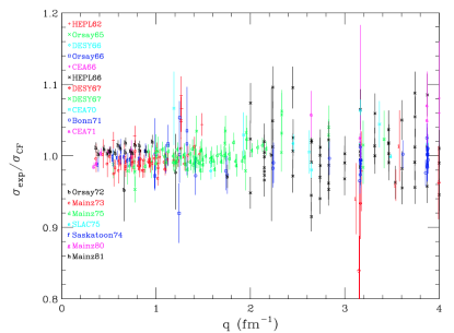
It may be useful to recall that the $p$-value of a data-set relative to a given assumption or fit –in this case the specified continued fraction– is the probability of obtaining data at least as incompatible with the hypothesis as the data actually observed. Let $f(\chi^{2},n_{\rm dof})$ be the $\chi^{2}$ probability distribution function. Let $\Gamma(a,b)\,[\Gamma(b)]$ be the incomplete [ordinary] gamma function. Then

$$p(\chi^{2},n_{\rm dof})=\int_{\chi^{2}}^{\infty}f(z,n_{\rm dof})\,dz={\Gamma(n_{\rm dof}/2,\chi^{2}/2)\over\Gamma(n_{\rm dof}/2)}$$ (15)

and $p(512,310)\!\simeq\!3.92\times 10^{-12}$, i.e. the quality of the fit in Sick is not “quite good”. It is possible Sick to reduce this behemoth disagreement by adding quadratically 3% to the Stanford error bars (to obtain $p(370,310)\!\simeq\!0.011$), or by a norm change of 1% of Simon … [which] would decrease $\chi^{2}$ by 60 (resulting in $p(452,310)\!\simeq\!2.38\times 10^{-7}$). Modifying the data is not necessarily a universally accepted procedure, or so would the corrected experimentalists opine.

It is also possible to draw sensible-looking curves through the data that, in their slope at ${\mathbf{q}}^{2}=0$, differ from a straight horizontal line in Fig. 1 by one or more of the $\sigma$’s in Eq. (2). The fact that the data points are very scattered is an unavoidable problem. One way to reconsider the issue is to take new and very precise data.

Figure 2: The lowest-energy Mainz data Mainz . The dark trumpet encompasses estimated theoretical and systematic uncertainties and $\pm 1\sigma$ statistical errors. Barred points are results of other experiments. The dotted lines are by-eye fits to data in the domain $\Delta Q^{2}=(\sim 0.06,0.2)$ (GeV/c)², for each of the sets of data. Their arrowy continuations are meant to illustrate how difficult it may be to extract from such an extrapolation the slope at the lowest-$Q^{2}$ measured point.

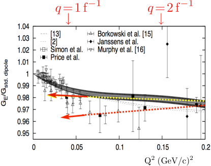
Such data exist Mainz and are partially reproduced in Fig. 2. The paper contains many relevant commentaries. One of them is: “The structure at small $Q^{2}$ seen in $G_{E}$ and $G_{M}$ corresponds to the scale of the pion of about $Q^{2}\approx m_{\pi}^{2}\approx 0.02$ (GeV/c²) and may be indicative of the influence of the pion clowd.” The most apposite remarks in Mainz concern the extraction of the results:

Two types of “flexible” models are considered in Mainz : fits to polynomials and spline fits. The $G_{E}$ results are

$$\sqrt{\langle r_{p}^{2}\rangle}\rm(spline)=\rm 0.875(5)_{stat}(4)_{syst}(2)_{model}\;\rm fm,$$

$$\sqrt{\langle r_{p}^{2}\rangle}\rm(polynom)=\rm 0.883(5)_{stat}(5)_{syst}(3)_{model}\;\rm fm$$ (16)

“Despite detailed studies the cause of the difference could not be found. Therefore, we give as the final result the average of the two values with an additional uncertainty of half of the difference”Mainz : the outcome quoted in Eq. (3). Whether the fits’ uncertainties are thus correctly estimated is debatable, but this is not the main point.

The crux of the matter is that the procedure in Mainz illustrates how, even for sets of “flexible” fits, the result is significantly set-dependent. The reason is simple: two analytic (or piece-wise analytic) functions arbitrarily close to each other in a given interval, say $\Delta Q^{2}=(Q^{2}_{\min},\infty)$, can be arbitrarily different in their continuation to another interval, such as $\Delta Q^{2}=(0,Q^{2}_{\min})$.

The data itself could be used to study the model-dependence of the extracted value of $\langle r_{p}^{2}\rangle$. Suppose that one fits the data in the interval $\Delta Q^{2}=(\sim 0.06,0.2)$ GeV² of Fig. 2 and extrapolates to the lowest-${\mathbf{q}}^{2}$ point at which there is still data and the $G_{E}$ slope is measured. This is analogous to extrapolating to ${\mathbf{q}}^{2}=0$, except in that the answer is known. A look at Fig. 2 suffices to conclude that the result is likely to be significantly wrong.

The “less flexible” models used to analyse the Mainz data have $\chi^{2}/n_{\rm dof}\approx 1.16$ to 1.29 for $n_{\rm dof}\approx 1400$ Mainz . The corresponding $p$-values range from $2.69\times 10^{-5}$ to $9.07\times 10^{-13}$. The most flexible ones have $\chi^{2}/n_{\rm dof}\approx 1.14$, or $p=1.88\times 10^{-4}$, that is, they are far from being flexible enough to describe the data. There seems to be a general tendency to forget that the quality of a fit is a function of two variables, not of their ratio, and that for large fixed $n_{\rm dof}$ the dependence of the fit’s quality on $\chi^{2}$ is an inordinately sharp function around $\chi^{2}=n_{\rm dof}$, suffice it to plot Eq. (15) to convince oneself.

VI The extraction of $\langle r_{p}^{3}\rangle_{(2)}$ from $ep$ scattering data

The result for the third Zemach moment is FriarSick

$$[\langle r_{p}^{3}\rangle_{(2)}]^{1/3}=(1.394\pm 0.022)\;\rm fm,$$ (17)

based on the data in Fig. 1. Based on the same data, the result for $\langle r_{p}^{2}\rangle$ is that of Eq. (2). To discuss the “third” moment, it is useful to write it in an alternative form:

$$\langle r_{p}^{3}\rangle_{(2)} \approxeq \int_{0}^{\infty}d{|\mathbf{q}}|\;I({\mathbf{q}}^{2})$$

$$I({\mathbf{q}}^{2}) \equiv {48\over\pi\,{\mathbf{q}}^{4}}\left[G_{E}^{2}({\mathbf{q}}^{2})-1+{{\mathbf{q}}^{2}\over 3}\,{\langle r_{p}^{2}\rangle}\right]$$ (18)

Notice that $I({\mathbf{q}}^{2})$ tends to a constant as ${\mathbf{q}}^{2}\to 0$.

The usual dipole form factor ($m_{d}^{2}=0.71$ GeV²) is a good-enough approximation for the forthcoming discussion. The shape of $I({\mathbf{q}}^{2})$ is shown in Fig. 3. Normalized to the total integral, the fractions of the integral in various relevant intervals $\Delta q=(a,b)$ fm^-1 are the following:

$$(0,0.4)\to 0.09\,;\;\;(0.6,1.6)\to 0.20\,;\;\;$$

$$(1.6,4)\to 0.29\,;\;\;(4,\infty)\to 0.38\,.$$ (19)

Figure 3: The third Zemach integrand of Eq. (18), illustrated for the usual dipole and shown in the same domain as that of Fig. (1). The shaded band is at $\Delta q=1.1\pm 0.5$ fm^-1. Data in the dashed extrapolation do not exist. The contributions to the moment from various intervals are discussed in the text.

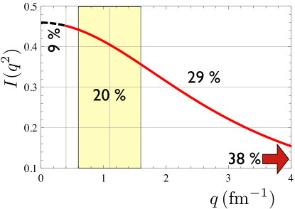
It is stated in FriarSick that “Sensitivity studies have shown that the main contribution to the integral comes from the region $\Delta q=(0.6,1.6)$ fm^-1 where the data base for electron-proton scattering is very good.” But the contribution is significantly larger in the range $\Delta q\times\rm fm=(1.6,4)$ where the data are particularly bad, see Fig. 1. The contribution if the range $(4,\infty)$ is even larger. The contribution in the range $(0,\sim 0.4)$, where there are simply no data, is not at all negligible. In other words, given the results in Eq. (19), the quoted statement must refer to the error estimate, not to the central value. And the basis for the deduced central value on $\langle r_{p}^{3}\rangle_{(2)}$ is still the fit in Fig. 1, whose $p$-value I have quoted.

It is concluded in another study CM of $I({\mathbf{q}}^{2})$ that “a large third Zemach moment can only occur if $\langle r_{p}^{4}\rangle$ is also large”. This is unobjectionable, though “large” means relative to the expectation from a dipole form-factor.

VII How to extract $r_{p}$ moments from $ep$ scattering data?

We have seen that the values and errors obtained in the literature for $\langle r_{p}^{2}\rangle$ and $\langle r_{p}^{3}\rangle_{(2)}$ are not credible. Since the various moments are highly correlated, another pertinent question is: how to draw, in the $(\langle r_{p}^{2}\rangle,\langle r_{p}^{3}\rangle_{(2)})$ plane, trustable, model-independent contour plots of given significance? A procedure might be the following:

(1) Normalize the data to a fixed model, as in Figs. 1,2.

(2) Study modifications, relative to the model, with a complete set of orthogonal functions, e.g. a discrete Fourier basis for the complete data interval, a function of a variable, such as $\log{\mathbf{q}}^{2}$, chosen to emphasize the most relevant, low-${\mathbf{q}}^{2}$, domain.

(3) Let the results fix the needed flexibility, i.e. cut the Fourier series at the term for which $\chi^{2}\leqslant n_{\rm dof}$ ($p\leqslant 0.5$).

(4) Sidestep an extrapolation to $\mathbf{q}\to 0$, which is unavoidably problematic. That is, use the data only where they exist. For this, one would have to Fourier transform $G_{E}(\mathbf{q})$ into $\rho(r)$ and study its moments. This is probably the only way of facing their unavoidable correlations.

(5) Show the correlated results as $(\langle r_{p}^{2}\rangle,\langle r_{p}^{3}\rangle_{(2)})$ contour plots for fixed acceptable values of $p$.

Such a procedure is very different from the usual. It may well lead to significantly different conclusions. Doing this analysis –in contrast to the simpler choice of verbally discussing it– is well beyond the scope of this paper.

VIII Discussion

The result of Eq. (1) is not only based on measurements including ordinary-hydrogen levels, but also on the $ep$-scattering result of Eq. (2), discussed in Section V. The elimination of this input from the CODATA fit to 78 (more or less) fundamental constants results in CODATA :

$$\sqrt{\langle r_{p}^{2}\rangle}(ep)=0.8737\pm 0.0075\;\rm fm$$ (20)

This result is shown as the shaded band in Fig. 4, displaying the rms radius versus the cubic root of the third Zemach moment. To facilitate the coming discussion, I have added the $-2\sigma$ and $-3\sigma$ lines corresponding to Eq. (20). Also shown in the figure are the two results, Eqs. (16), of the Mainz experiment Mainz .

Figure 4: Atomic data for the rms radius versus the third Zemach moment. The “$\mu H$” curve is the correlation between the rms radius and the third Zemach moment implied by the observation of Eq. (6) and the theoretical result of Eq. (21). Also shown are the polynomial and spline results of Mainz (meant to be read as horizontal bands) and the $\langle r_{p}^{3}\rangle_{(2)}$ of FriarSick .

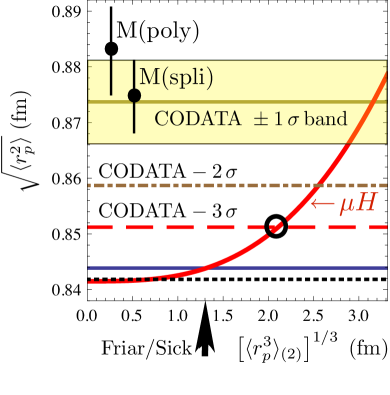
The lowest (dashed) line in Fig. 4 is Eq. (10), from the $\mu H$ Lyman shift Pohl . The continuous straight line above the previous one takes into account the renormalization correction of Eq. (13). Make the same correction in Eq. (6) to obtain:

$$\!\!\!\!\!\!L^{\rm th}\left[\langle r_{p}^{2}\rangle,\langle r_{p}^{3}\rangle_{(2)}\right] =$$

$$\!\!\!\!\!\!209.9779(49) - 5.20123\,\langle r_{p}^{2}\rangle+0.00913\,\langle r_{p}^{3}\rangle_{(2)}$$ (21)

and equate it to the observed value of Eq. (5) to obtain the “$\mu H$” correlation, the continuous curve in Fig. 4. This correlation –and not a figure for $r_{p}$– is the outcome of the theoretical analysis of the measurement Pohl .

If the value of the third Zemach moment was that of Eq. (17), indicated by an arrow in Fig. 4, the muonic- and ordinary-hydrogen results would be more than $3\sigma$ away. If, instead, $(\langle r_{p}^{3}\rangle_{(2)})^{1/3}\sim 2.1$ fm the tension would diminish to the $3\sigma$-level, marked by a circle in Fig. 4 (the increase of the moment is more severe than it seems to be, since the observable is not its cubic root).

The standard deviations of the previous paragraph are the ones pertinent to a normal data distribution, for which $\pm 1$, $\pm 2$ and $\pm 3\sigma$ correspond to coverage probabilities of 68.27%, 95.45% and 99.73%. But the data of CODATA are not normally distributed, meaning that the bands of the same fixed probability are not the ones in Fig. 4, and that the conclusions of the previous paragraph should be correspondingly weakened.

More precisely, 9 out of 135 input data in CODATA –related to the Watt balance, the lattice spacing in various Silicon crystals, the molar volume of the same element and the quotient of Plank’s constant to the neutron mass) have had their uncertainties increased by a multiplicative factor 1.5 CODATA . This choice helps in obtaining a fairly satisfactory overall $p$-value, $p=0.221$, but it describes a hypothetical set of experiments, not the actual one. Moreover, the question of the individual $p$-values of the experiments is not reexamined in CODATA . We have seen examples of how misleading this omission may be.

Figure 5: The CODATA result of Eq. (20), the $\mu H$ correlation also shown in Fig. 4, and recent “theory-driven” results for $\langle r_{p}^{2}\rangle$ (meant to be horizontal bands). B1, B2 cite DispersionRelations , HP1 to HP4 cite HP and WLTY quotes WLTY .

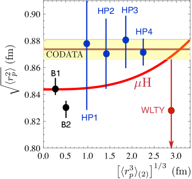
A solidly-motivated approach to the extraction of $\langle r_{p}^{2}\rangle$ from the $ep$ scattering data is based on the use of the analytical properties of the nucleon’s form factors. Two recent examples are DispersionRelations ; HP (it would be helpful to know the $p$-values of these fits). Their $r_{p}$ outcomes are shown in Fig. 5. The result of a first-principle lattice calculation WLTY is also shown. The spread of the theoretical results may be indicative of the difficulty of reaching a consensus. Should the spread reflect a level of uncertainty, there is no “tension” between theory and observations.

IX Conclusions

We have seen that, to the precision required to analyse the recent muonic-hydrogen results, the vintage “wave-function at the origin” expression for the Lamb shift, Eq. (11), is insufficiently precise. In configuration space this is because the wave function is not only probed at the origin, but up to distances at which details of the proton charge distribution (beyond its mean square radius) become relevant. Thus the model-dependence of the correction, see Eqs. (13,12).

Translated into momentum space, the previous paragraph becomes very familiar. A wave function at the “origin”, a $\delta(\vec{0})$, corresponds to a uniform sampling of all momentum transfers, something that an atom can hardly provide. The correction, a proper match of renormalisation scales, can be phrased as a proton’s running radius. Not a surprising result: in a field theory all measured quantities are scale-dependent.

The above correction to the analysis in Pohl reduces its disagreement with the $\langle r_{p}^{2}\rangle$ CODATA result from $\sim 5\,\sigma$ to at most $\sim 4\,\sigma$. The “at most” is crucial, for the conclusion depends on the value adopted for the third Zeemach moment. We have seen that its extraction from $ep$ scattering data is most questionable. In Fig. 4 one can see that, even after the corrections I have discussed, $(\langle r_{p}^{3}\rangle_{(2)})^{1/3}\sim 3$ fm would be required to have ordinary and muonic hydrogen precisely agree. Even if a dipole form factor is only a very vague description of the data, such a value feels unexpectedly large, part of the argument in CM .

The Lamb shift measurement provides a correlation between the two relevant moments: the narrow curved domain labeled “$\mu H$” in Fig. 4. It would be very helpful to extract the correlation dictated by $ep$ data, to be added as confidence-level contours to the figure, to decide –with confidence– what the empirical conclusion is. It may well be that the $\mu H$ and $ep$ correlations have a sufficient overlap for the question of data incompatibility to be moot. After all, also for $ep$ scattering, the two quantities plotted in Fig. 4 are obviously strongly correlated, a fact that has been totally ignored.

Similar inferences can be extracted from the comparison of theory and data summarized in Fig. 5. Currently none of these “theory-driven” results are available in the form of two-dimensional $(\langle r_{p}^{2}\rangle,\langle r_{p}^{3}\rangle_{(2)})$ confidence-level plots. Even barring other putative limitations of current theory or experimental analyses, the most extreme views on the subject at hand rpADR ; Flowers seem to have been largely exaggerated.

Acknowledgments

I am grateful to Shelly Glashow, Maurizio Pierini, Chris Rogan and Maria Spiropulu for their comments and to Pietro Slavich for finding an error in Yo1 .

References

- (1) R. Pohl, et al. Nature 466 (2010) 213. R. Pohl, et al., Supplementary Information, doi: 10.1038/nature09250.
- (2) P. J. Mohr, B. N. Taylor & D. B. Newell, Rev. Mod. Phys. 80 (2008) 633.
- (3) A. De Rújula, Phys. Letts. B 693 (2010) 555.
- (4) J. Flowers, Nature 466 (2010) 195.
- (5) Bernauer et al. arXiv:1007.5076v2 (2010).
- (6) M. I. Eides, H. Grotch & V. A. Shelyuto, Springer Tracts in Mod. Phys. 222 (Springer, Berlin Heidelberg, 2007). S. G. Karshenboim, Phys. Rep. 422 (2005) 1.
- (7) M. Niering, Phys. Rev. Lett. 84 (2000) 5496. B. de Beauvoir, Eur. Phys. J. D 12 (2000) 61. C. Schwob Phys. Rev. Lett. 82 (1999) 4960.
- (8) I. Sick, Phys. Lett. B 576 (2003) 62.
- (9) P. G. Blunden & I. Sick, Phys. Rev. C 72 (2005) 057601.
- (10) S. G. Karshenboim, Phys. Rep. 422 (2005) 1. K. Pachucki, Phys. Rev. A60 (1999) 3593. E. Borie, Phys. Rev. A 71 (2005) 032508. A. P. Martynenko, Phys. Rev. A 71 (2005) 022506. A. P. Martynenko, Phys. At. Nucl. 71 (2008) 125. K. Pachucki & U. D. Jentschura, Phys. Rev. Lett. 91 (2003) 113005.
- (11) J. L. Friar & I. Sick Phys. Rev. A 72 (2005) 040502(R).
- (12) A. De Rújula, Phys. Rev. Lett. 32 (1974) 1143. The argumentation in this paper was strengthened in A. De Rújula, H. Georgi & H.D. Politzer, Ann. Phys. (N.Y.) 103 (1977) 315; Phys. Lett. 64B (1976) 428. For a lighter discussion, see A. De Rújula in 50 Years of Yang-Mills Theory, edited by G. ’t Hooft. World Scientific Publishing Co. Singapore, 2005, page 401.
- (13) D. J. Gross & S. B. Treiman, Phys. Rev. Lett. 32 (1974) 1145.
- (14) H. D. Politzer, Phys. Rev. Lett. 26 (1973) 1346. D. Gross & F. Wilczek, Phys. Rev. Lett. 26 (1973) 1343. G. ’t Hooft, unpublished.
- (15) G.G. Simon, et al., Nucl. Phys. A 364 (1981) 285.
- (16) I. C. Clet & G. A. Miller, arXiv:1008.4345v3.
- (17) M. A. Belushkin, H. W. Hammer & U. G. Meissner, Phys. Rev. C 75 (2007) 035202.
- (18) R. G. Hill & G. Paz, arXiv:1008.4619v1.
- (19) P. Wang et al., Phys. Rev. D 79 094001 (2009).
- (20) A. De Rújula, arXiv:1010.3421.