UNIVERSITY OF OKLAHOMA
GRADUATE COLLEGE

A DISSERTATION
SUBMITTED TO THE GRADUATE FACULTY
in partial fullfillment of the requirements for the
Degree of
DOCTOR OF PHILOSOPHY
By

Norman, Oklahoma
2010

A DISSERTATION APPROVED FOR THE
HOMER L. DODGE DEPARTMENT OF PHYSICS AND ASTRONOMY
BY

                                                            

Dr. Howard Baer, Chair

                                                            

Dr. Kimball Milton

                                                            

Dr. Phillip Gutierrez

                                                            

Dr. Eddie Baron

                                                            

Dr. Nikola Petrov

© Copyright by  2010
All Rights Reserved.

In loving memory of my father,
Dr. Raj.

Abstract

In this thesis we examine three different models in the MSSM context, all of which have significant supergravity anomaly contributions to their soft masses. These models are the so-called Minimal, Hypercharged, and Gaugino Anomaly Mediated Supersymmetry Breaking models. We explore some of the string theoretical motivations for these models and proceed by understanding how they would appear at the Large Hadron Collider (LHC). Our major results include calculating the LHC reach for each model’s parameter space and prescribing a method for distinguishing the models after the collection of 100 ${\textrm{fb}^{-1}}$ at $\sqrt{s}=14$ TeV. AMSB models are notorious for predicting too low a dark matter relic density. To counter this argument we explore several proposed mechanisms for $non$-$thermal$ dark matter production that act to augment abundances from the usual thermal calculations. Interestingly, we find that future direct detection dark matter experiments potentially have a much better reach than the LHC for these models.

1 Introduction

Particle physics is at an exciting point at the time of writing this thesis. The long-awaited start of the Large Hadron Collider (LHC) era has finally begun with the first collection of data at the world-record breaking collision energy of 7 TeV c.o.m. in March of this year. After the first two years the experiment is planned to run at the full design luminosity accumulating ultimately 100-1000 ${\textrm{fb}^{-1}}$ at a tremendous $\sqrt{s}=$ 14 TeV. It is expected, or at least hoped, that the LHC will shed light on important mysteries of the Standard Model (SM) of particle physics by allowing us to detect particle states that have yet to be observed at the Tevatron. The most likely of these is the Higgs boson, the remaining piece of the SM, which is thought to be responsible for the spontaneous breaking of the electroweak symmetry. The presence of the Higgs boson in the SM is itself a strong theoretical motivator that other heavy particle states exist that can also be discovered at the LHC. One very well-motivated class are the supersymmetric (SUSY ) particle states whose masses lie in the TeV range. The discovery of these particles at the LHC would have deep implications for the nature of space-time. Having the potential to discover new physical states such as these puts us at a truly unique and exciting time.
On the other hand particle physics is also merging increasingly with cosmology. The energy density of the Universe is known to be comprised of Dark Energy (71%), normal baryonic matter (4%), and a non-luminous form of matter known as Dark Matter (DM) which comprises roughly 25% of the energy density. If DM is considered to be comprised of particles, it must be massive to account for the relic abundance and it must be cold enough to allow for structure formation on large scales. For these reasons, there are no good candidates for DM in the SM. There is, however, a particularly good DM candidate in supersymmetric theories in which R-parity is conserved. The particle is the lightest neutralino, and the search for it is an important priority at the LHC and in DM experiments around the world.
The outline of this thesis is as follows. The remainder of the Introduction is intended to provide background for subsequent chapters. We will first give a $very$ brief introduction to the Standard Model (SM) and simultaneously attempt to motivate supersymmetry. Next, we will introduce the idea of the scalar superfield before moving on to describe the Minimal Supersymmetric Standard Model (MSSM). Once the fields and interactions of the theory are established, we turn our attention to how the scalar superpartners of the SM acquire mass at the weak scale. These quantities are usually given by a combination of low-energy constraints ($e.g$, electroweak symmetry breaking parameters, $etc.$) and by high-scale physics ($M_{GUT}$, $M_{string}$, $etc.$) that relates to physics at the low scale ($M_{weak}$) through renormalization group effects. For this thesis, the latter quantities are, in part, due to anomalies that are present in supergravity theories, and a rather technical derivation of these will be given Section 1.4. Theories in which contributions of this type are important will be referred to as “Anomaly-Mediated Supersymmetry Breaking (AMSB) models”. The Introduction concludes with descriptions of the computational tools used in this work and should be used for reference in the chapters that follow.
In Chapters 2 - 4 we will examine three different models of the AMSB type. The first is the prototypical model known as the $minimal$ AMSB model, and is “minimal” in the sense that it has the minimum ingredients to be phenomenologically viable. The second model is referred to as “Hypercharged AMSB” (HCAMSB) because it pairs AMSB mass contributions with $U(1)$-contributions at the string scale. The third model is actually a class of string theory models with specific high-scale boundary conditions and a rather $low$ string scale, referred to collectively as “Gaugino AMSB”, or “inoAMSB” for short. Each of these chapters gives a full theoretical explanation of the model being considered. They also give a full analysis for LHC physics, that is, we describe all renormalization group effects, compute weak-scale parameters, run signal and SM-background simulations for $pp$ collisions at $\sqrt{s}=14$ TeV, and calculate the reach of the models’ parameters for 100 ${\textrm{fb}^{-1}}$ of accumulated data (one year at full design luminosity).
It would be greatly insufficient to focus only on collider physics searches since future cosmological data will be precise enough to be competitive. In Chapter 5 we consider the question of dark matter (DM) in AMSB models where we take the lightest neutralino to be our DM candidate. AMSB models notoriously yield too little thermally-produced relic abundance to account for the measured DM. However, it is expected that other heavy particles present in the early universe could increase the DM abundance in AMSB models $non$-$thermally$. In this chapter we present several such scenarios and assume the total DM abundance can be accommodated. After a review of DM theory and direct/indirect detection experiments, we calculate important rates for AMSB DM cosmology for all of the models in Chapters 2 - 4. We supplement all rates with detailed physical explanations. We also find the reach for each model and compare the results with LHC expectations.
Finally, we conclude with a general overview of the results in Chapter 6.

1.1 Standard Model and Supersymmetry

So far most experimental data in HEP experiments is described by the Standard Model of particle physics and this has been the case for 30+ years. The basic facts of this model are given in this section with the goal in mind of extending it to include supersymmetry.
The Standard Model is a collection of three identical generations of spin-$\frac{1}{2}$ fermion fields, spin-1 vector bosons, and spin-0 scalar Higgs fields. The fermions interact through the exchange of spin-1 vector bosons that arise through the gauge invariance of both abelian and non-abelian interactions. The interactions of the particles can be trivial or non-trivial under each of the $SU(3)_{c}$, $SU(2)_{L}$, and $U(1)_{Y}$ rotations, where “c” stands for the color-charge and “L” for the weak-isospin, and “Y” is the hypercharge of the interacting particles.
Those particles that interact through $SU(3)_{c}$ interactions are the spin-$\frac{1}{2}$ fermions known as quarks and the interaction is mediated by spin-1, color-charged octet of gluon fields. Fermions that are unaffected by $SU(3)_{c}$ interactions are known as leptons. Left-handed fermions interact in very specific pairs (or doublets) and the mediators of the interactions are the spin-1 triplet of $W_{\mu}$-bosons. These interactions do not apply to right-handed fermions, and they are the only sources of flavor-change in the SM [8] as is described, for example, by Cabibbo-Kobayashi-Maskawa mixing for quarks. And finally, all fermions are charged under abelian $U(1)_{Y}$ rotations, and these interactions are mediated by the $B_{\mu}$ vector boson.
The inclusion of a Higgs particle is necessary to give mass to both the weak sector bosons and matter fields. The Higgs ($\Phi={\phi^{+}\choose\phi^{0}}$) is thought to be a dynamic field with quartic self-interactions, thus its contribution to the Lagrangian is

$${\cal L}_{Higgs}=|\partial_{\mu}\Phi|^{2}+\mu^{2}\Phi^{\dagger}\Phi-\lambda(\Phi^{\dagger}\Phi)^{2}.$$ (1.1)

By allowing $\Phi$ to be a complex doublet that transforms non-trivially under the electroweak symmetry, $SU(2)_{L}\times U(1)$, the covariantized action mixes the Higgs with weak and hypercharge bosons [90]. When the neutral Higgs acquires a VEV, the $SU(2)\times U(1)_{Y}$ symmetry is still a good symmetry of the Lagrangian, yet its generators no longer annihilate the vacuum. The symmetry is said to be broken $spontaneously$, and the remnant symmetry is the $U(1)_{em}$ of electromagnetism. In the symmetry breaking process, massless degrees of freedom are produced which are subsequently transformed into the longitudinal modes of the electroweak bosons (rendering them massive). Also upon acquiring a VEV, the Higgs gives mass to the fermion fields through its Yukawa couplings to matter.
The fundamental particles of the Standard Model are summarized in Table 1.1 along with the matter and Higgs quantum numbers. The table tells how the particles transform under a given symmetry. For example, left-handed fermions form doublets transforming non-trivially under $SU(2)$, right-handed fermions are singlets under $SU(2)$, and quarks transform as a triplet of color charge under $SU(3)$. Not shown in the table are two other generations of fermions, identical to the one shown with exactly the same quantum numbers, but with larger masses. Also, anti-particles have not been included.

				Symmetry/Quantum #s
Fermion	Flavor			$SU(3)_{c}$	$SU(2)_{L}$	$U(1)_{Y}$
leptons	${\nu_{e}\choose e}_{L}$			1	2	-1
	$e_{R}$			1	1	-2
quarks	${u\choose d}_{L}$			3	2	$\frac{1}{3}$
	$u_{R}$			3	1	$\frac{4}{3}$
	$d_{R}$			3	1	$\frac{2}{3}$
Higgs	$\Phi={\phi^{+}\choose\phi^{0}}$		gauge  $\Biggl{\{}$	gluon	weak	hypercharge
boson				$G_{\mu}^{A}$	$W_{\mu}^{i}$	$B_{\mu}$
	(1,2,1)			$A=1\cdots 8$	$i=0,+,-$

Table 1.1: Matter, vector boson, and Higgs fields in the Standard Model.

The SM is completely consistent but there are several reasons why it cannot be the complete description of nature. A list of some, but not all, of these reasons are given here:

• hierarchy problem - radiative corrections to the scalar (Higgs) mass terms are quadratically divergent due to gauge and fermion loops, but unitarity arguments require the mass to be constrained to less than a few hundred GeV [20]. If the SM is to be considered an effective field theory below a high-scale $\Lambda$, then the Higgs mass could be subject to excessive and unnatural fine-tuning.

• Dark Matter (DM) is not yet included in the SM.

• Gravitational interactions are not present in the SM.

It is ideal to have a single framework that can address these issues, and in this thesis supersymmetry is the adopted solution. A supersymmetry transformation acts on bosonic state to form fermionic states and vice versa. The hierarchy problem is famously solved in supersymmetric theories because the fermion loop corrections to the Higgs mass are accompanied by bosonic corrections. The new loops are also quadratically divergent but generally appear with opposite sign. In the case of $unbroken$ supersymmetry, where fermions and bosons have equal mass, the fermionic and bosonic contributions precisely cancel one another to all orders of perturbation theory [20][82][101]. Even in the case of broken supersymmetry, the divergent contributions to the Higgs mass are at most logarithmic and, therefore, not severely destabilizing.
Supersymmetry also provides a framework for addressing the remaining two issues in the list above. In particular, we will consider $local$ supersymmetry at a very high scale that naturally incorporates gravity. It will be necessary for the supersymmetry to be (spontaneously) broken to agree with phenomenology. When we define the minimal supersymmetric model and renormalize the model parameters at the weak scale, we will encounter natural EW symmetry breaking, non-quadratically divergent scalar masses, and supersymmetry provides several DM candidates.
Before developing the superfield formalism in the next section, it is important to discuss some technical details regarding why, if supersymmetry is to explain the short-comings of the SM, it must be a broken symmetry. Since the supersymmetry generators transform bosons into fermions, they must be fermionic and therefore obey $anti$-commutation relations. When these relations are combined with the Poincaré algebra, the closed ($graded$) algebra that results is known as the super-Poincaré algebra. The squared-momentum generator, $(P^{\mu})^{2}$, is a Casimir of the super-Poincaré algebra [81], and so supersymmetric fermion-boson pairs are expected to be degenerate. If this was a rigid requirement, supersymmetry would already by excluded by the fact that no partners of the SM particles have been observed with identical mass. Supersymmetry necessarily has to be a $broken$ symmetry to be phenomenologically viable.
Viable supersymmetric models must assume breaking in a way that does not re- introduce quadratic divergences. In order for this to occur it is necessary for the dimensionless couplings of the theory to be unmodified by supersymmetry breaking, and that only couplings with positive mass dimension are included in the supersymmetry breaking potential. Supersymmetry that is broken in this way is said to be broken softly. This reduces the number of additional terms that can be included in the soft supersymmetry-breaking Lagrangian, ${\cal L}_{soft}$, which are: linear (gauge singlet), bilinear (including masses), and trilinear ($A$-term) scalar interactions, and bilinear gaugino mass terms.

1.2 Superfields

In this section we briefly review some aspects of the superfield formalism. We will see how boson-fermion pairs are embedded into super-multiplets. Also in this section, key ingredients to supersymmetric theories are defined, and the notation to be used in describing the minimal supersymmetric standard model of the next section are established.
Superfields place boson fields in the same multiplet as their fermionic partners. It is convenient to introduce anti-commuting Grassmann variables arranged as Majorana spinors, $\theta\ (\bar{\theta})$, that multiply the fields in order to put them on the same footing. Fields in a super-multiplet that are not multiplied by Grassmann variables are referred to as the “lowest” component, those with one Grassmann variable are the second component, $etc$ . It is the lowest component that determines the type of superfield, $i.e.$, scalar, spinor, vector, etc.
A general scalar superfield has many components as seen in

$$\hat{\Phi}(x,\theta)= S-i\sqrt{2}\bar{\theta}\gamma_{5}\psi-\frac{i}{2}(\bar{\theta}\gamma_{5}\theta)M-\frac{1}{2}(\bar{\theta}\theta)N+\frac{1}{2}(\bar{\theta}\gamma_{5}\gamma_{\mu}\theta)V^{\mu}$$ (1.2)

$$+i(\bar{\theta}\gamma_{5}\theta)[\bar{\theta}(\lambda+\frac{i}{\sqrt{2}}\not{\partial}\psi)-\frac{1}{4}(\bar{\theta}\gamma_{5}\theta)^{2}[D-\frac{1}{2}\nabla^{2}S]],$$

but this representation is not irreducible. Fortunately supersymmetry allows for chiral representations of superfields. For example, there is a representation where the scalar component and the left-chiral spinor transform into one another without mixing with the corresponding right-handed fields. A left chiral scalar superfield is of the form

$$\hat{S}_{L}(x,\theta)=S(\hat{x})+i\sqrt{2}\bar{\theta}\psi_{L}(\hat{x})+i\bar{\theta}\theta_{L}F(\hat{x})\\$$ (1.3)

where the lowest (Grassmann) component is a scalar, the second component is the partner fermion, and F is an auxiliary field required to balance off-shell degrees of freedom. Similarly a right chiral scalar superfield is of the form

$$\hat{S}_{R}(x,\theta)=S(\hat{x}^{{\dagger}})-i\sqrt{2}\bar{\theta}\psi_{R}(\hat{x}^{{\dagger}})+i\bar{\theta}\theta_{R}F(\hat{x}^{{\dagger}}),\\$$ (1.4)

but will frequently be recast as the conjugate of a left-chiral scalar field. In short-hand, chiral scalar superfields can be referred to by their components, ($S,\psi_{L},F$). To be clear, the scalar component is not a spinor and does not have helicity. It contains the annihilation operator of the superpartner of a chiral fermion. Under supersymmetry transformations the components of the left-chiral superfield transform into one another:

$$\delta S =-i\sqrt{2}\bar{\alpha}\psi_{L}$$ (1.5)

$$\delta\psi_{L} =-\sqrt{2}F\alpha_{L}+\sqrt{2}\not{\partial}S\alpha_{R}$$ (1.6)

$$\delta F =i\sqrt{2}\bar{\alpha}\not{\partial}\psi_{L}.$$ (1.7)

It is intriguing that the $F$-term of the superfield transforms as a total derivative (Equation (1.7)) because field combinations that transform as total derivatives bring dynamics to the action. This property of the $F$- term is true even of products of chiral superfields because, as can be shown, they are themselves chiral superfields. The general polynomial of left-chiral superfields is another left-chiral superfield known as the $superpotential$, and its $F$-term ($\bar{\theta}\theta_{L}$-component) must be appended to the Lagrangian. In a renormalizable theory, the superpotential is at most a cubic polynomial by dimensional analysis.
It can also be shown that the $(\bar{\theta}\gamma_{5}\theta)^{2}$-component, or “$D$-term”, of a general superfield (Equation (1.2)) transforms as a total derivative under supersymmetry transformations . The product of chiral superfields, however, does not have an interesting $D$-term because it is already a total derivative, as in

$$\hat{S_{L}}\ni\frac{1}{8}(\bar{\theta}\gamma_{5}\theta)^{2}\nabla^{2}S.$$ (1.8)

This term is automatically zero in the action and does not produce any dynamics, and is for this reason that the superpotential does not contribute $D$-terms. However, a polynomial of mixed chirality can give important $D$-term contributions to the Lagrangian, and this function is referred to as the Kähler potential. It is important to note that the Kähler potential is at most quadratic by renormalizability and real by hermiticity of the Lagrangian [20]. It is then taken to have the form

$$K=\sum_{i,j=1}^{N}A_{ij}\hat{S}_{i}^{\dagger}\hat{S}_{j},$$ (1.9)

the $D$-term of which is also included in the Lagrangian as with the $F$-term contributions.

1.3 Minimal Supersymmetric Standard Model

We are now ready to build the minimal extension of the Standard Model (SM) that incorporates supersymmetry, the Minimal Supersymmetric Standard Model (MSSM). That is, we seek the minimal extension of the SM that includes broken supersymmetry, and that is both phenomenologically and theoretically safe. In order to do this, it is first assumed that the theory will have the SM gauge symmetry group: $SU(3)_{c}\times SU(2)_{L}\times U(1)$. Thereafter, all gauge and matter fields of the SM must be promoted to superfields. The matter superfields must be L-chiral fields as required by the superpotential. Thus, for each $chirality$ of every SM fields, we will choose there will be one $left$-chiral superfield assigned.
Extending the SM Higgs field to a superfield will add a partner fermion, a higgsino ($\tilde{h}$). Having only one extra fermion re-introduces $U(1)^{3}_{Y}$ and $U(1)_{Y}SU(2)^{2}_{L}$ gauge anomalies [99] that are canceled successfully in the SM. If instead there are two Higgs doublets in the theory, with opposite hypercharges, $Y=1$ and $Y=-1$, their fermionic partners have the correct quantum numbers to satisfy the anomaly cancellation. Furthermore, a single Higgs doublet is not allowed in the MSSM because the lower-component fermions of the SM weak doublets would receive their mass from the conjugate of the Higgs, which is a $right$-chiral superfield. Interactions of $right$-chiral superfields are forbidden in the superpotential [20], and we are forced to accept at least two Higgs doublets into the MSSM. We denote by $\hat{H}_{u}$ the Higgs doublet of superfields that is associated with the mass of $Y=1$ fermions, and $\hat{H}_{d}$ associated with mass of $Y=-1$ fermions. The matter and Higgs superfields of the MSSM are shown in Table 1.2.

Field	$SU(3)_{C}$	$SU(2)_{L}$	$U(1)_{Y}$
$\hat{L}$=$\hat{\nu}_{eL}\choose\hat{e}_{L}$	1	2	-1
$\hat{E^{c}}$	1	1	2
$\hat{Q}$=$\hat{u_{L}}\choose\hat{d_{L}}$	3	2	$\frac{1}{3}$
$\hat{U}^{c}$	3∗	1	$-\frac{4}{3}$
$\hat{D}^{c}$	3∗	1	$\frac{2}{3}$
$\hat{H}_{u}$=$\hat{h}_{u}^{+}\choose\hat{h}_{u}^{0}$	1	2	1
$\hat{H}_{d}$=$\hat{h}_{d}^{-}\choose\hat{h}_{d}^{0}$	1	2∗	-1

Table 1.2: Matter and Higgs superfields in the MSSM.

Next it is necessary to define the superpotential of the theory. The superpotential, denoted by $\hat{W}$, contains $SU(2)\times U(1)$ invariant combinations of chiral matter superfields and Higgs fields. The matter fields are coupled to Higgs fields through Yukawa coupling matrices, while the $\mu$-term couples $H^{u}$ and $H^{d}$. In the MSSM it is:

$$\hat{W}=\mu\hat{H}_{u}^{a}\hat{H}_{da}+\sum_{i,j=1,3}[({\bf f}_{u})_{ij}\hat{Q}_{i}^{a}\hat{H}_{ua}\hat{U}_{j}^{c}+({\bf f}_{d})_{ij}\hat{Q}_{i}^{a}\hat{H}_{da}\hat{D}_{j}^{c}+({\bf f}_{e})_{ij}\hat{L}_{i}^{a}\hat{H}_{da}\hat{E}_{j}^{c}],$$ (1.10)

where $a$ is an $SU(2)$ index and $c$ stands for conjugation.
This superpotential is not completely general because, in its construction, terms that would lead to baryon (B) and/or lepton (L) number violation have been carefully omitted. There are renormalizable terms that could be added that are gauge and supersymmetrically invariant, but the presence of these terms would have physical consequences that are highly constrained by experiment (for instance, proton decay). The omission of these operators is made possible by imposing a discrete symmetry on the superpotential, known as R-parity. When

$$R=(-1)^{3(B-L)+2s}$$ (1.11)

is conserved ($s$ is the spin of the state), renormalizable $B$- and $L$-violating interactions will be forbidden . Furthermore, conservation of R-parity leads to three important consequences [99]:

• superpartners will always be produced in $pairs$ at colliders;

• the decays of the SM superpartners (including extra higgsinos) produce an odd number of the final state lightest SUSY particle (LSP), which for our purposes this is a neutralino;

• the LSP is absolutely stable and therefore may be a good dark matter candidate.

We accept R-parity as part of the definition of the MSSM and should stay mindful of these consequences in the coming chapters.
The final step in constructing the MSSM is to include all gauge-invariant soft supersymmetry-breaking terms into the Lagrangian. These terms are thought to arise from the interactions between MSSM fields and a “hidden” sector where SUSY is broken (see Section 1.4). These terms raise the masses of supersymmetric partners of the SM fields and are needed for electroweak symmetry breaking (see next subsection). The MSSM soft Lagrangian is [20]

$${\cal L}_{soft}= -\bigl{[}{\tilde{Q}}_{i}^{\dagger}{\bf m^{2}_{Q}}_{ij}{\tilde{Q}}_{j}+{\tilde{d}}_{Ri}^{\dagger}{\bf m^{2}_{D}}_{ij}{\tilde{d}}_{Rj}+{\tilde{u}}_{Ri}^{\dagger}{\bf m^{2}_{U}}_{ij}{\tilde{u}}_{Rj}+$$

$$\qquad{\tilde{L}}_{i}^{\dagger}{\bf m^{2}_{L}}_{ij}{\tilde{L}}_{j}+{\tilde{e}}_{Ri}^{\dagger}{\bf m^{2}_{E}}_{ij}{\tilde{e}}_{Rj}+m_{H_{u}}^{2}|H_{u}|^{2}+m_{H_{d}}^{2}|H_{d}|^{2}\bigr{]}$$

$$-\frac{1}{2}\bigl{[}M_{1}\bar{\lambda_{0}}\lambda_{0}+M_{2}\bar{\lambda_{A}}\lambda_{A}+M_{3}\bar{{\tilde{g}}}_{B}{\tilde{g}}_{B}\bigr{]}$$

$$-\frac{1}{2}\bigl{[}M^{\prime}_{1}\bar{\lambda_{0}}\gamma_{5}\lambda_{0}+M^{\prime}_{2}\bar{\lambda_{A}}\gamma_{5}\lambda_{A}+M^{\prime}_{3}\bar{{\tilde{g}}}_{B}\gamma_{5}{\tilde{g}}_{B}\bigr{]}$$

$$+\bigl{[}({\bf a_{u}})_{ij}\epsilon_{ab}{\tilde{Q}}_{i}^{a}H_{u}^{b}{\tilde{u}}_{Rj}^{\dagger}+({\bf a_{d}})_{ij}{\tilde{Q}}_{i}^{a}H_{da}{\tilde{d}}_{Rj}^{\dagger}+({\bf a_{e}})_{ij}{\tilde{L}}_{i}^{a}H_{da}{\tilde{e}}_{Rj}^{\dagger}+h.c.\bigr{]}$$

$$+\bigl{[}({\bf c_{u}})_{ij}\epsilon_{ab}{\tilde{Q}}_{i}^{a}H_{d}^{*b}{\tilde{u}}_{Rj}^{\dagger}+({\bf c_{d}})_{ij}{\tilde{Q}}_{i}^{a}H_{*ua}{\tilde{d}}_{Rj}^{\dagger}+({\bf c_{e}})_{ij}{\tilde{L}}_{i}^{a}H_{ua}^{*}{\tilde{e}}_{Rj}^{\dagger}+h.c.\bigr{]}$$

$$+\bigl{[}bH_{u}^{a}H_{da}+h.c.\bigr{]}.$$ (1.12)

In short, the parameters above are the scalar mass matrices of lines 1 & 2, the gaugino mass terms of lines 3 & 4, the trilinear $A$-term couplings from supersymmetry breaking in line 5, trilinear terms of line 6 & 7. It is seen that these terms give the MSSM an extremely large number of parameters. We will see that in AMSB-type models the number of parameters will be reduced from the 178 in the soft Lagrangian above to just a few. This is one of the many attractive features of the class of models considered in this thesis.

Electroweak Symmetry Breaking in the MSSM

As in the Standard Model, the electroweak symmetry is spontaneously broken by minimizing the potential in the scalar sector. We have seen that due to supersymmetry the scalar sector includes much more than just the Higgs particle. The potential is extended now to include effects of all matter scalars along with all possible effects that originate in SUSY breaking. The scalar potential is then the sum of the various terms:

$$V_{MSSM}=V_{F}+V_{D}+V_{soft}$$ (1.13)

with

$$V_{F} =\sum_{i}|F_{i}|^{2}=\sum_{i}\ \Bigl{|}\frac{\partial W}{\partial\hat{S}_{i}}\Bigr{|}^{2}_{\hat{S}=S},\qquad\textrm{and}$$ (1.14)

$$V_{D} =\frac{1}{2}\sum_{A}\Bigl{[}\sum_{i}\hat{S}_{i}^{\dagger}gt_{A}S_{i}\Bigr{]}^{2},$$ (1.15)

and $V_{soft}$ comes from lines 1, 2, 5, 6, and 7 of Equation (1.12). As in the SM, the Higgs VEVs should be responsible for the breaking. In the usual manner, gauge symmetry allows the VEV of $H_{u}$ to be rotated to its lower neutral component. Upon minimizing with respect to the other component of $H_{u}$, it is necessarily so that $\langle h_{d}^{-}\rangle$ = 0 [20]. Then only the potential of the neutral Higgs fields needs to minimized in the breaking of electroweak symmetry. In this way, provided no other scalars are allowed to develop VEVs, only charge-conserving vacuua can occur in the MSSM.
It will be important to understand how the electroweak symmetry is broken properly in order to put constraints on parameters in a model. Schematically the minimization requires the following:

• the potential is extremized with respect to both $h_{u}^{0}$ and $h_{d}^{0}$ and their conjugates through its first derivatives, i.e.

  $\frac{\partial V}{\partial h_{i}^{0}}\textrm{ (and conjugates)}=0;$

• to ensure that EW-breaking occurs the origin must be a maximum, i.e., the determinant of the Hessian should be negative there, and this imposes the condition

  $(B\mu)^{2}>(m_{H_{u}}^{2}+\mu^{2})(m_{H_{d}}^{2}+\mu^{2});$

• and finally, in order that the potential is bounded from below the (D-term) quartic terms must be non-zero (positive at infinity) and this results in the condition

  $2|B\mu|<m_{H_{u}}^{2}+m_{H_{d}}^{2}+2\mu^{2}.$

Electroweak symmetry is broken properly when these conditions are met because a well-defined minimum develops that does not break charge. It is customary to define the ratio of the Higgs VEVs as

$\textrm{tan}\ \beta=\bigl{(}\frac{v_{u}}{v_{d}}\bigr{)}$,

and to recast the important potential minimization conditions as

$$B\mu=\frac{(m_{H_{u}}^{2}+m_{H_{d}}^{2}+2\mu^{2})\textrm{sin}2\beta}{2}\quad\textrm{and}$$ (1.16)

$$\mu^{2}=\frac{m_{H_{d}}^{2}-m_{H_{u}}^{2}(\textrm{tan}\ \beta)^{2}}{\textrm{tan}^{2}\beta-1}-\frac{M_{Z}^{2}}{2},$$ (1.17)

where $M_{Z}=\frac{g^{2}+g^{\prime 2}}{2}(v_{u}^{2}+v_{d}^{2})$ is the tree-level result for the $Z^{0}$ mass when the effects of EW-breaking on gauge bosons are considered.
In the SM, the required shape of the potential is achieved through the inclusion of a tachyonic scalar that transforms non-trivially under the EW symmetry and acquires a VEV. The same is true in the MSSM, with the exception that the potential is generated naturally at the weak scale through RGE effects rather than put in by hand. As SUSY parameters are evolved from the GUT scale down to the weak scale, the large top Yukawa coupling drives the up-type squared Higgs mass to negative values, thus triggering what is know as radiative electroweak symmetry breaking (REWSB).
The $\mu$ value calculated through Equation 1.17 is purely phenomenological. In actuality, it is difficult to understand why $\mu$ should be so small considering it appears in a supersymmetric superpotential term and should naturally be of order the (high) supersymmetry breaking scale (perhaps of order the Planck scale, $M_{\rm{Pl}}$) [38], but such high values would destroy the mechanism of electroweak symmetry breaking. This is known as the “$\mu$-problem”. Typically the low $\mu$ value is assumed to arise by some other mechanism, most commonly that of Guidice and Masiero [59].
The procedure described above is true in general for minimizing the scalar potential, however there are important cases where radiative corrections need to be considered. For example, without radiative corrections, the MSSM would already be excluded by Higgs mass bounds. For the sake of brevity we do not dwell on these corrections, but their importance is noted.
Now that we have seen the MSSM and its parameters, we can determine the physical mass eigenstates that are important for any type of phenomenology. The following subsections give a general overview of the contributions to the mass matrices at the weak scale in the various sectors.

Neutralinos and Charginos

The spontaneous electroweak symmetry breaking leads to mixing of fields with the same electric charge, spin, and color quantum numbers. The spin-$\frac{1}{2}$, color-neutral fermions mix and come as wino-bino-higgsino mass eigenstate combinations. Those combinations that are neutral are called neutralinos and those that are charged are charginos.
The Lagrangian mass terms for the neutral fields can be written as

$${\cal L}_{neutralino}=-\frac{1}{2}\bar{\Psi}{\cal M}_{neutralino}\Psi$$ (1.18)

where $\Psi^{T}=({\tilde{h}}_{u}^{0},{\tilde{h}}_{d}^{0},{\tilde{W}}^{3},{\tilde{b}})$ contains the neutral up- and down-type higgsinos, wino, and bino respectively. The tree-level mass matrix for this sector is

$${\cal M}_{neutralino}=\left(\begin{array}[]{cccc}0&\mu&-\frac{gv_{u}}{\sqrt{2}}&\frac{g^{\prime}v_{u}}{\sqrt{2}}\\ \mu&0&\frac{gv_{d}}{\sqrt{2}}&-\frac{g^{\prime}v_{d}}{\sqrt{2}}\\ -\frac{gv_{u}}{\sqrt{2}}&\frac{gv_{d}}{\sqrt{2}}&M_{2}&0\\ \frac{g^{\prime}v_{u}}{\sqrt{2}}&-\frac{g^{\prime}v_{d}}{\sqrt{2}}&0&M_{1}\\ \end{array}\right).$$ (1.19)

After diagonalizing the mass matrix we find the mass eigenstates, ${\tilde{Z}}_{i}$, in linear combinations of the higgsinos and gauginos, ${i.e.}$,

$${\tilde{Z}}_{i}=v_{i(1)}{\tilde{h}}_{u}^{0}+v_{i(2)}{\tilde{h}}_{d}^{0}+v_{i(3)}{\tilde{W}}^{3}+v_{i(4)}{\tilde{b}}$$ (1.20)

Note that the neutralino mass matrix is hermitian and will have real eigenvalues.
Charginos are linear combinations of the charged gauginos, ${\tilde{W}}^{\pm}$, and charged higgsinos, ${\tilde{h}}_{u}^{-}$ and ${\tilde{h}}_{d}^{+}$. They appear in the Lagrangian as

$${\cal L}_{chargino}=-\bar{\Phi}({\cal M}_{charged}P_{L}+{\cal M}_{charged}^{T}P_{R})\Phi,$$ (1.21)

where the negatively charged, two-component field is $\Phi^{T}=(\frac{\lambda_{1}+{\it i}\lambda_{2}}{2},P_{L}{\tilde{h}^{-}}_{d}-P_{R}{\tilde{h}^{+}}_{u})$, and the tree-level matrix is

$${\cal M}_{charged}=\left(\begin{array}[]{cc}M_{2}&-gv_{d}\\ -gv_{u}&-\mu\\ \end{array}\right).$$ (1.22)

The diagonalization of ${\cal M}_{charged}$ is more involved than in the neutral case as it requires two unitary matrices, U and V, and this procedure can be found in [20]. In the end, there are two mass eigenstates for each charge in the combinations

$${\tilde{W}}_{i}^{-}=U_{i(1)}{\tilde{W}}^{-}+U_{i(2)}{\tilde{h}}_{u}^{-}$$ (1.23)

$${\tilde{W}}_{i}^{+}=V_{i(1)}{\tilde{W}}^{+}+V_{i(2)}{\tilde{h}}_{d}^{+}.$$ (1.24)

The physics mass eigenvalues will depend on $\mu$, $M_{2},M_{W}$, and $\textrm{tan}\ \beta$. Note that the mass matrix is tree-level and loop corrections are not shown here.
In general, there may be a high degree of mixing for any of the neutralino and chargino mass eigenstates. It turns out that of the parameters $\mu,M_{1},M_{2}$, and $\textrm{tan}\ \beta$ that contribute to the mixing, AMSB type models tend to have a very light $M_{2}$ value. This results in both the lightest neutralino and lightest chargino being wino-like, a fact that will have strong implications for LHC phenomenology (Chapters 2- 4) and Dark Matter (Chapter 5) as we will see.

Sfermion Masses

Unlike the SM, there are four mass contributions to the squarks and sleptons. They are: superpotential contributions that rely and Higgs VEV; generational soft masses from SUSY breaking; trilinear interactions with Higgs fields; and D-term contributions. The result of these contributions is to mix left and right sfermions of the same flavor with $2\times 2$ matrices that are straight-forwardly diagonalized. The procedure is not very illuminating for the current discussion, and the reader is referred to [20] [82] for more discussion. In the end, the mass eigenvalues will depend on $\mu,\textrm{tan}\ \beta$, trilinear couplings, SM EW parameters, and the corresponding fermion mass.

Gluino Mass

The gluino mass is not tied to the EW symmetry breaking sector, and its presence is purely due to supersymmetry breaking and renormalization, and is parameterized by $M_{3}$. The gluino must be a mass eigenstate because it is the only color octet fermion and $SU(3)_{C}$ is not a broken symmetry. In the next section we will see how this and other gaugino masses are generated by anomalous SUGRA effects.

1.4 Supergravity Soft Terms

The MSSM is considered to be an effective theory containing information about supersymmetry breaking through the soft terms of Equation (1.12). In this section the origin of the soft terms is outlined. Most importantly, the explanation of how the supergravity anomaly imparts mass is explained. The class of models where these contributions dominate (or is comparable to) all other forms of soft mass generation are known as Anomaly Mediated Supersymmetry Breaking Models, and all of the models in this thesis are of this type.
It has already been remarked that the generators of supersymmetry transformations are spinors, and it follows that the variational parameter of supersymmetry is also a spinor. When supersymmetry is “localized” and combined with the symmetries of general relativity, the resulting theory is called supergravity [52][102][82]. Supergravity has a supermultiplet of gauge particles: the spin-2 graviton, and its super-partner, the spin-$\frac{3}{2}$ gravitino, both of which are massless so long as supersymmetry is unbroken. However, when supersymmetry is broken spontaneously by the VEV of the auxiliary component of a “hidden” supermultiplet X, $i.e.$, $<F_{X}>$, a massless goldstone fermion, or $goldstino$, is produced. This goldstino becomes the longitudinal mode of the gravitino thereby imparting mass, and this mechanism is called the $super$-$Higgs$ mechanism due to its obvious parallels to SM Higgs mechanism. The gravitino mass, $m_{3/2}$, is given by

$$m_{3/2}=\frac{<F_{X}>}{\sqrt{3}M_{\rm{Pl}}},$$ (1.25)

and plays a key role in soft mass generation when supersymmetry breaking is communicated to the MSSM particles. In the case of gravity-mediated supersymmetry breaking, MSSM fields interact with the hidden sector mainly through gravitational interactions. These interactions induce soft masses for the scalars that are suppressed by powers of $M_{\rm{Pl}}$ and typically of the order [99]

$$m_{soft}\sim\frac{<F_{X}>}{M_{\rm{Pl}}}.$$ (1.26)

When the MSSM is coupled to gravity, the effective soft Lagrangian below the Planck scale is given as in Equation (1.12) with coefficients that depend on powers of $m_{\rm{soft}}\sim m_{3/2}$. However these tree-level effects can be suppressed relative to the quantum anomaly contributions to be described in the next subsection, and we will see that these contributions will require typically higher values of $m_{3/2}$ than is typical for gravity mediated scenarios.

Anomaly Mediated Supersymmetry Breaking

In this section we examine how soft masses are generated by anomalous supergravity (local susy) effects. Low-energy type II-B string theory enforces the following functional as the classical Wilsonian action for a generic super Yang-Mills coupled to gravity (see [55][102] for more discussion):

$$S= -3\int d^{8}z{\bf E}~{}exp\{-\frac{1}{3}K(\Phi,\bar{\Phi};Q,\bar{Q}e^{2V})\}$$ (1.27)

$$\quad+\quad\bigl{(}\int d^{6}z{\cal E}~{}[W(\Phi,Q)+\frac{1}{4}f_{ab}{\cal W}^{a\alpha}{\cal W}^{b}_{\alpha}]+h.c.\bigr{)}$$

$$\quad+({\rm higher\ order\ derivatives}),$$

where K is the Kähler potential, W the superpotential, $f_{ab}$ are the gauge coupling, and ${\cal W^{\alpha}}$ is the gauge field strength associated with the prepotential V. R is the chiral curvature superfield, E is the full superspace measure, and ${\cal E}$ is the chiral superspace measure.
The issue of the anomaly arises with the first term in the functional above because it is not in the standard form with Einsteinian gravity. It also has the improper form for kinetic metric, given by the second derivative of the Kähler potential. What is desired instead is to have the fields transformed out of the SUGRA frame (as it appears in (1.27)) into the more physical Einstein-Kähler frame that has Einsteinian gravity as well as canonical matter normalizations. The supergravity effects are disentangled via Weyl-rescaling of the metric, i.e.,

$$g_{mn}=\hat{g}_{mn}\cdot e^{-\frac{1}{3}K},$$ (1.28)

and by rescaling fermion fields by exponentials of $K$ in order that fermions and bosons belonging to the same supermultiplet are normalized in the same way [102][68].
The torsion and the chirality constraints of supergravity (SUGRA) are invariant under Weyl transformations, given by re-weightings with parameter $e^{\tau}$ and $e^{\bar{\tau}}$, where $\tau$ is a chiral superfield. Some of these transformations are given below:

${\bf E}\rightarrow e^{2(\tau+\bar{\tau})}{\bf E}$,   $\cal E$$\rightarrow$$e^{6\tau}$$\cal E$,

$V\rightarrow V$,  $\nabla_{\alpha}\rightarrow e^{\tau-2\bar{\tau}}(\nabla_{\alpha}+...)$,

$\Phi\rightarrow\Phi$,  $Q\rightarrow Q$,  &   $W_{\alpha}\rightarrow e^{-3\tau}W_{\alpha}.$

The SUGRA action itself is not invariant under these transformations. However, we can make insertions of the “Weyl compensator”, $C$, such that the action is invariant:

$$S=-3\int d^{6}z{\cal E}~{}(\frac{-\bar{\nabla}^{2}}{4}+2R)~{}C\bar{C}~{}exp\{-\frac{1}{3}K(\Phi,\bar{\Phi};Q,\bar{Q}e^{2V})\}$$ (1.29)

$$\quad+\quad\bigl{(}\int d^{6}z{\cal E}~{}[C^{3}W(\Phi,Q)+\frac{1}{4}f_{ab}{\cal W}^{a\alpha}{\cal W}^{a}_{\alpha}]+h.c.\bigr{)}.$$

The invariance under Weyl symmetry is established by the following transformations for the compensator:

$C\rightarrow e^{-2\tau}C$.

Because it does not appear in the action with derivatives, it is not a propagating degree of freedom and the action is completely equivalent to the case without the use of a compensator. This internal symmetry is broken when $<C>\neq 0$ (however the actual value does not matter as it can be chosen to be anything), but the breakdown is to nothing.
At the quantum level, however, the measure is not invariant due to the chiral anomaly [7] for matter fermions, $\Psi$:

$$d[\Psi]\rightarrow d[\Psi]exp\Bigl{\{}\frac{3c_{a}}{16\pi^{2}}\int dz^{6}{\cal E}~{}2\tau{\cal W}^{\alpha}{\cal W}_{\alpha}+h.c.,\Bigr{\}}$$ (1.30)

with

$$c_{a}=T(G_{a})-\sum_{r}T_{a}(r),$$ (1.31)

where $T_{a}(r)$ is the trace over the squared-generator matter representation a, and $T(G_{a})$ is the trace over the adjoint squared generator. In order to maintain local Weyl invariance, this anomaly must be canceled by the replacement

$$f_{a}(\Phi)\rightarrow{\tilde{f}}_{a}=f_{a}(\Phi)-\frac{3c_{a}}{8\pi^{2}}~{}{\rm ln}C.$$ (1.32)

This ensures that the original SUGRA action of Equation (1.27) is equivalent to the Weyl symmetric action Equation (1.29). We can see that in the gauge $C=1$, the effect is nil and we are in the original SUGRA frame. The Kähler -Einstein frame corresponds to the choice

$${\rm log}~{}C+{\rm log}~{}\bar{C}=\frac{1}{6}K|_{\rm harmonic}~{},$$ (1.33)

where on the right we take only the piece that is the sum of chiral plus anti-chiral parts.
We must also do matter field redefinitions in order for them to have canonical normalizations. To do this we expand the Kähler potential in matter fields

$$K({\Phi,\bar{\Phi},Q,\bar{Q}e^{2V}})=K_{m}(\Phi,\bar{\Phi})+Z_{I\bar{J}}\bar{Q}^{\bar{J}}e^{2V}Q^{I}+\dots.$$ (1.34)

For simplicity we consider a single matter field multiplet in representation r (the case of more fields is easily generalizable) and find that the kinetic terms are contained in

$$\int dz^{8}{\bf E}C\bar{C}e^{-\frac{1}{3}K_{m}}Z_{r}(\Phi,\bar{\Phi})\bar{Q}e^{2V}Q,\quad Z_{r}=Z_{r}^{\dagger}.$$ (1.35)

If one does a field transformation of the form $Q\rightarrow e^{\tau_{Z}}Q$, the functional measure is again not invariant. This results in the Konishi anomaly [76][97] with another contribution to the measure of the form [46]

$$exp\Bigl{\{}\frac{-T_{a}}{16\pi^{2}}\int dz^{6}{\cal E}~{}2\tau_{Z}{\cal W}^{\alpha}{\cal W}^{\alpha}+h.c.\Bigr{\}}.$$ (1.36)

This subsequently implies redefining the gauge coupling function:

$$H_{a}\equiv f_{a}(\Phi)-\frac{3c_{a}}{8\pi^{2}}~{}{\rm ln}C-\frac{T_{a}(r)}{4\pi^{2}}\tau_{Z}.$$ (1.37)

We then get canonical normalization of the matter kinetic term,

$$\int dz^{8}{\bf E}C\bar{C}e^{-\frac{1}{3}K_{m}}e^{\tau_{Z}+\bar{\tau}_{Z}}Z_{r}(\Phi,\bar{\Phi})\bar{Q}e^{2V}Q,$$ (1.38)

by simply making the choice

$$\tau_{Z}+\bar{\tau}_{Z}={\rm ln}(C\bar{C}e^{-\frac{1}{3}K_{m}}Z_{r})|_{harmonic}.$$ (1.39)

This together with the appropriate gauge coupling redefinition, Equation (1.37), ensures that the action remains locally Weyl invariant.
The final step is to determine the gauge couplings and gaugino masses as they relate to the auxiliary components of all fields, $viz.$, compensator, moduli, and matter fields. Denote the lowest component of the transformed gauge coupling function (Equation (1.37)) by $h_{a}=H_{a}|$, and its real part by $h_{aR}=\Re H_{a}|$. The mass and gauge coupling are related by

$$\frac{m_{a}}{g_{a}^{2}} =\Re[F^{i}\partial_{i}f_{a}(\Phi)]|-\frac{b_{a}}{8\pi^{2}}\frac{F^{C}}{C}-\frac{T_{a}(r)}{4\pi^{2}}F^{i}\partial_{i}({\rm ln}(e^{1\frac{1}{3}K_{m}}Z))|$$ (1.40)

$$=\Re[F^{i}\partial_{i}f_{a}(\Phi)]|-\frac{c_{a}}{8\pi^{2}}F^{i}\partial_{i}K_{m}-\frac{T_{a}(r)}{4\pi^{2}}F^{i}\partial_{i}({\rm ln}Z_{r}))|,$$

where $i$ is for all moduli of the underlying string theory. In going to the second line we have imposed the Einstein-Kähler gauge by using the F-component of Equation (1.33). The gauge coupling on the other hand is given by $g_{a}^{-2}=h_{aR}$ and in the Einstein-Kähler frame it is

$$g_{a}^{-2}=\Re f(\Phi)|-\frac{c_{a}}{16\pi^{2}}K_{m}|-\frac{T_{a}(r)}{8\pi^{2}}{\rm ln}Z_{r}|.$$ (1.41)

Then, when considering F-type breaking, these expressions give the appropriate gaugino masses and gauge couplings after the Kähler potential and the original gauge coupling function ($f_{a}$) of the theory have been specified.
Suppose the theory has a cut-off $\Lambda$, and we wish the renormalize the gaugino masses and the gauge couplings by evaluating them at a scale $\mu$. This is done by shifting the Wilsonian gauge coupling function by a finite (1-loop) renormalization,

$$H_{a}(\Phi,\tau,\tau_{Z})\rightarrow H_{a}(\Phi,\tau,\tau_{Z},\mu)=H_{a}(\Phi,\tau,\tau_{Z})-\frac{b_{a}}{8\pi^{2}}{\rm ln}\frac{\Lambda}{\mu},$$ (1.42)

and re-evaluating the expressions (here, the $b_{a}$ values are the $\beta$- function coefficients). However, the gauge couplings we have derived until this point are not physical because the kinetic terms for the gauge fields are not normalized properly. We again must do a rotation into the proper frame, but this time of the gauge fields. The details are omitted here, but the result is only to shift $\Re H_{a}$ by again using a new chiral superfield transformation parameters, $\tau_{Z}$ (see [9][46] for details):

$$\Re H_{a}\rightarrow\Re H_{a}-\frac{T_{a}}{8\pi^{2}}\Re\tau_{V}=\frac{1}{g_{phys}^{2}}.$$ (1.43)

It is important to stress that this derivation of the soft mass contributions has made no impact on the scalar sector of the theory. The “Weyl” anomaly is often referred to as the “rescaling” anomaly referring to the fact that many authors have renormalized gauge couplings with an implicit compensator field associated with the mass scale of the theory, $i.e.$, $\beta$-function running appears usually as ${\rm ln}(\frac{|C|\Lambda}{\mu})$ instead of as it is seen in Equation (1.42) (without $|C|$). It is this fact that has led authors to derive soft contributions for the $scalars$ of the theory in addition to gaugino masses [94]. However, it has been argued strongly in [46] that the problem with the usual derivation is that it is based on conformal invariance rather than strictly on Weyl invariance alone. It is ultimately argued in that paper that the Weyl anomaly does not contribute at all to scalar masses.
In this thesis, a somewhat impartial approach is taken regarding the puzzles surrounding the anomaly. The models that are examined in the following chapters will have anomaly contributions as prescribed in the “usual” derivations (mAMSB and HCAMSB) that include scalar masses (resulting from anomaly rescaling) that evolve as

$$m_{i}^{2}\propto\frac{d\gamma_{i}}{d\ {\rm log\mu}}m_{3/2}^{2},$$ (1.44)

where $\gamma_{i}$ is the anomalous dimension. We also consider cases that contain anomaly soft contributions to gauginos as advocated by de Alwis [46], as it is in the inoAMSB class. In all cases considered here, upon supersymmetry breaking, the relation (1.40) implies soft gaugino masses of the form

$$M_{a}=\frac{b_{a}g_{a}^{2}}{16\pi^{2}}m_{3/2},\ \ a=1,2,3,$$ (1.45)

with $b_{a}=(\frac{33}{5},1,-3)$. In any case, we will see that the various models will be distinguishable at the LHC, at least at the 100${\textrm{fb}^{-1}}$ level with $\sqrt{s}=$ 14 TeV.

1.5 Computational Tools

Renormalization Group Equations

As described earlier in this Introduction, inputs at the high-scale (the GUT or string scales for instance) are required as boundary conditions for evolution of soft SUSY breaking parameters. These parameters then are used in determining physical mass parameters at the TeV scale by matching the MSSM renormalization group equations (RGEs) with low energy boundary conditions, i.e., weak-scale gauge and third generation Yukawa couplings.
All of the RGE parameter solutions in this research are obtained through an up-down iterative matching procedure using the Isasugra subprogram of Isajet v7.79 [88]. Isasugra implements a full two-loop RGE running of the MSSM parameters in the $\overline{DR}$-scheme using Runge-Kutta integration. The iteration starts with high-precision weak-scale gauge and Yukawa couplings, runs up to the the high scale where the user parameters are used as inputs, and then returns to the weak scale. At the end of the iteration, MSSM masses are recalculated and the RGE-improved 1-loop corrected Higgs potential is minimized. The $\beta$-functions are also re-evaluated at each threshold crossing during each iteration. The iterations terminate at the prescribed level of convergence, which is that all RGE solutions except $\mu$ and $B\mu$ are within 0.3% of the last iteration. Because of their rapid variation at the weak-scale, the latter are required to have convergence at the 5% level.
Isajet v7.79 has the mAMSB and HCAMSB models coded into it. No extra coding was necessary for inoAMSB as the high-scale inputs are non-universal gaugino masses in the ratio 6.6:1:-3 as usual for AMSB, while all scalar and $A$-parameters inputs are highly suppressed, i.e., zero. For convenience, the parameters of each of the three models described in this work are listed in Table 1.3.

Model	Parameters
mAMSB:	$m_{0},m_{3/2},\textrm{tan}\ \beta,sign(\mu)$
HCAMSB:	$\alpha,m_{3/2},\textrm{tan}\ \beta,sign(\mu)$
inoAMSB:	$m_{3/2},\textrm{tan}\ \beta,sign(\mu),$
	$(M_{1},M_{2},M_{3})=(6.6,1,-3)\times m_{3/2}$

Table 1.3:

Event Simulation

Isajet 7.79 - 7.80 is used for the simulation of signal and background events at the LHC. A toy detector simulation is employed with calorimeter cell size $\Delta\eta\times\Delta\phi=0.05\times 0.05$ and $-5<\eta<5$. The hadronic calorimeter (HCAL) energy resolution is taken to be $80\%/\sqrt{E}+3\%$ for $|\eta|<2.6$ and forward calorimeter (FCAL) is $100\%/\sqrt{E}+5\%$ for $|\eta|>2.6$. The electromagnetic (ECAL) energy resolution is assumed to be $3\%/\sqrt{E}+0.5\%$. We use the UA1-like jet finding algorithm GETJET with jet cone size $R=0.4$ and require that $E_{T}(jet)>50$ GeV and $|\eta(jet)|<3.0$. Leptons are considered isolated if they have $p_{T}(e\ or\ \mu)>20$ GeV and $|\eta|<2.5$ with visible activity within a cone of $\Delta R<0.2$ of $\Sigma E_{T}^{cells}<5$ GeV. The strict isolation criterion helps reduce multi-lepton backgrounds from heavy quark ($c\bar{c}$ and $b\bar{b}$) production.
We identify a hadronic cluster with $E_{T}>50$ GeV and $|\eta(j)|<1.5$ as a $b$-jet if it contains a $B$ hadron with $p_{T}(B)>15$ GeV and $|\eta(B)|<3$ within a cone of $\Delta R<0.5$ about the jet axis. We adopt a $b$-jet tagging efficiency of 60%, and assume that light quark and gluon jets can be mis-tagged as $b$-jets with a probability $1/150$ for $E_{T}<100$ GeV, $1/50$ for $E_{T}>250$ GeV, with a linear interpolation for $100$ GeV$<E_{T}<$ 250 GeV [65].
Isajet is capable of generating events for a wide variety of models. Once the parameters of the theory are defined, RGE evolution determines weak scale masses and $2\rightarrow 2$ processes are weighted by their cross sections and generated.
In addition, background events are generated using Isajet for QCD jet production (jet-types include $g$, $u$, $d$, $s$, $c$ and $b$ quarks) over five $p_{T}$ ranges as, for example, in Tables 3.4 and 4.3. Additional jets are generated via parton showering from the initial and final state hard scattering subprocesses. Also generated are backgrounds in the $W+jets$, $Z+jets$, $t\bar{t}(173.1)$ and $WW,\ WZ,\ ZZ$ channels. The $W+jets$ and $Z+jets$ backgrounds use exact matrix elements for one parton emission, but rely on the parton shower for subsequent emissions.

Dark Matter

For all the models considered in this work, to calculate the relic density of neutralinos and direct detection rates we used, respectively, the IsaRED and IsaRES subroutines of the IsaTools package found in Isajet [88]. To calculate indirect detection rates following from neutralino scattering, annihilation, and co-annihilations, the DarkSUSY [60] package was used. DarkSUSY, by default, uses the Isasugra subprogram of Isajet v7.69 [88] to calculate the SUSY spectrum, with exception to Higgs masses for which it uses FeynHiggs [61]. In order to perform the calculations for our particular models, we transplanted the Isajet v7.79 code into the DarkSUSY package.

2 Minimal AMSB

With the origin of the anomaly contributions to the particle spectrum understood we can now look at models with high scale inputs that are connected to the TeV scale through renormalization group running. The first model we encounter has been analyzed extensively in the literature [30][87] and will serve as the model of comparison for the other AMSB models to be considered. The model is known as the $Minimal$ Anomaly Mediated Supersymmetry Breaking Model (mAMSB) and its most important aspects, relevant for LHC and DM considerations, are highlighted in this chapter.
The mAMSBmodel has the attractive feature that it depends on only a few GUT-scale input parameters:

$$m_{0},m_{3/2},\textrm{tan}\ \beta,\ {\rm and\ sign}(\mu),$$ (2.1)

each of which have been mentioned in Chapter 1 except for $m_{0}$, which will be discussed shortly. As discussed in Section 1.4, the AMSB contributions to the gaugino masses are given by

$$M_{1} =\frac{33}{5}\ \frac{g_{1}^{2}}{16\pi^{2}}m_{3/2}^{2}$$ (2.2)

$$M_{2} =\ \ \ \ \frac{g_{2}^{2}}{16\pi^{2}}m_{3/2}^{2}$$ (2.3)

$$M_{3} =-3\frac{g_{3}^{2}}{16\pi^{2}}m_{3/2}^{2},$$ (2.4)

where $g_{i}$ are the running MSSM gauge couplings. Furthermore, the scalar masses and trilinear parameters are given by

$$m_{{\tilde{f}}}^{2} =-\frac{1}{4}\{\frac{d\gamma}{dg}\beta_{g}+\frac{d\gamma}{df}\beta_{f}\}m_{3/2}^{2}\ \ {\rm and}$$ (2.5)

$$A_{f} =\frac{\beta_{f}}{f}\frac{m_{3/2}}{16\pi^{2}},$$ (2.6)

where $\beta_{g}$ and $\beta_{f}$ are, respectively, the gauge coupling and Yukawa coupling $\beta$-functions, and their correspond $anomalous\ dimensions$ are denoted by $\gamma$. Note that the above soft terms are parametrically tied to supersymmetry-breaking through $m_{3/2}$ (Section 1.4). Also note that all of the above equations are valid at $any$ scale.
There are several phenomenologically important points to be made about the AMSB contributions.

• Anomaly contributions to scalars are the same for particles with the same quantum numbers, while first and second generation Yukawa couplings are negligible. In the case that AMSB dominates the soft contributions, flavor-violation is safely avoided. In Figure 2.1, the running of the soft parameters $M_{1},M_{2},M_{3}$, the third generation squark doublet mass ($\sqrt{m^{2}_{{\tilde{Q}}_{3}}}$), the right-handed sbottom mass ($\sqrt{m^{2}_{{\tilde{b}}_{R}}}$), and the bottom trilinear parameter ($A_{b}$) are shown. There is implicit dependence on $A_{b}$ in both of the squark mass parameters.

  

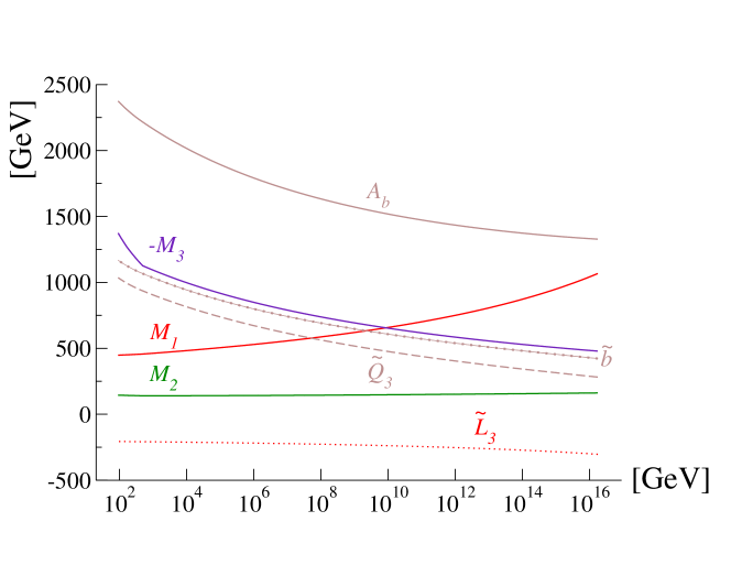
  Figure 2.1: Running of soft parameters to the weak scale in the mAMSB scenario for the point ($m_{0}$, $m_{3/2}$, $\textrm{tan}\ \beta$) = (0 GeV, 50 TeV, 10) with $\mu>0$.

• The anomaly contributions to scalars are partially determined by anomalous dimensions, which are negative for sleptons. After RGE running to the weak scale, sleptons remain with negative masses (see Figure ${\tilde{L}}_{3}$ in 2.1). The $minimal$ solution to this problem is to introduce the ad hoc parameter, $m_{0}$, in 2.1 at the $GUT$-scale to prevent tachyonic sleptons at the weak scale. This is achieved simply by adding $m_{0}^{2}$ to all scalar squared-masses and the $m_{0}$ value is taken as a free parameter of the mAMSBmodel.

• Scalars with different helicities are nearly (left/right) degenerate at the weak scale in the mAMSBmodel. This is despite possible splitting at the $GUT$ scale. This is demonstrated in Figure 2.2 where, for example, selectrons and up- squarks masses are run from the $GUT$ scale to the weak scale for a mAMSB point with $m_{0}$=300 GeV, $m_{3/2}=$ 50 TeV, $\textrm{tan}\ \beta=10$, and $\mu>0$. While left and right sparticle masses are split at the high scale, the evolution (accidentally) drives them closer at lower scales.

  

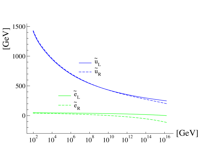
  Figure 2.2: Demonstration of near-degeneracy of left and right superparticles at weak scale in the mAMSB scenario for the point ($m_{0}$, $m_{3/2}$, $\textrm{tan}\ \beta$) = (300 GeV, 50 TeV, 10) with $\mu>0$.

• Requiring weak-scale gaugino masses places $m_{3/2}$ at much higher values than in other supersymmetry-breaking scenarios. With $m_{3/2}\sim O(10-100)$ TeV range, gravitinos have a short enough lifetime to avoid the gravitino problem [74][77][91].

• After evaluating gaugino masses at the weak scale (Equations (2.2 - 2.4) ), $|M_{2}|$ is invariably the lightest of them (see Figure 2.1). This, along with the potential minimization conditions, affects the diagonalization of the neutralino and chargino mass matrices of Equations (1.19) and (1.22) to produce $wino$-like lightest mass-eigenstates in both cases. Thus ${\tilde{Z}}_{1}$ and ${\tilde{W}}_{1}$ have nearly degenerate masses in AMSB type models.

This last point is particularly important because it potentially allows for a discrimination between AMSB and other types of supersymmetry-breaking effects at the LHC. Denote the mass difference between the lightest chargino and the lightest neutralino, $m_{{\tilde{W}}_{1}}-m_{{\tilde{Z}}_{1}}$, by $\Delta M_{{\tilde{Z}}_{1}}$. As $\Delta M_{{\tilde{Z}}_{1}}$ decreases, the chargino decay width decreases and its lifetime becomes longer. Thus, there is a possibility of detecting ${\tilde{W}}_{1}$s as highly ionizing tracks (HITS) in LHC detectors.
$\Delta M_{{\tilde{Z}}_{1}}\sim O({\rm MeV})$ splittings are rather small but ${\tilde{W}}_{1}$ can usually decay to e or $\mu$ through the three-body process ${\tilde{W}}_{1}\rightarrow e\nu{\tilde{Z}}_{1}$. When the gap opens beyond the pion mass ($\sim$ 140 MeV) hadronic decays of the chargino are allowed [42][78]. Further enlarging the mass gap leads to channels with 2$\pi$ and 3$\pi$ final states. The ${\tilde{W}}_{1}$ width would be smallest when it decays to a single lepton and obviously grows as other channels open. Chargino detection then falls into two categories [30]:

• $\Delta M_{{\tilde{Z}}_{1}}<m_{\pi^{+}}$ : $\pi$ decay modes are unavailable and ${\tilde{W}}_{1}$ can leave a track far out in the muon chambers!

• $m_{\pi^{+}}<\Delta M_{{\tilde{Z}}_{1}}<200$ MeV : high $p_{T}$ charginos decay in the inner detector region. The decays ${\tilde{W}}_{1}\rightarrow\pi^{\pm}{\tilde{Z}}_{1}~{}$ and ${\tilde{W}}_{1}\rightarrow l\nu{\tilde{Z}}_{1}~{}$ are accessible with $l$ and $\pi$ emitted softly. This regime has a clear signal. The charginos appear as highly ionizing tracks in the inner detector and decays to SM particles. But the SM particles are too soft for energy deposits in the Ecal or the Hcal and appear to contribute to the missing energy already taken away by the ${\tilde{Z}}_{1}$. This leads to an observable HIT that terminates, or a stub, and large amounts of $\not{E}_{T}$.

We will come back to this in Chapters 3 and 4 when we discuss the LHC phenomenology of AMSB models at greater depth.

3 Hypercharged AMSB

3.1 Introduction to the HCAMSB Model

Hypercharged anomaly-mediation is composed of two mechanisms that induce masses for visible sector matter fields. The soft masses come from the anomaly mediation already discussed and an additional $U(1)$ mediation, and the latter depends intricately on a particular D-brane setup. While this form of mediation is not general in the way that anomaly contributions are, it is an interesting pathway to understanding how D-brane constructions can impact the visible sector. In the next section the description of how the $U(1)$ gives masses to MSSM fields is given. Then the $U(1)$ will be paired with AMSB to give the full HCAMSB model. Following the next section the phenomenology of the model will be discussed.

3.2 Geometrical Setup with D-branes

There should be some comments made about D-branes first because the model relies on them. D-branes are extended objects on which strings can terminate with ‘D’irichlet boundary conditions. For this discussion we consider only type IIB string theory with Dp-branes that have $p=1-9$, odd. These branes fill the usual 3+1 space-time, but can have superfluous dimensions that must be wrapped by internal cycles to make them effectively invisible. A D7 brane, for example, requires a 4-cycle wrapped within the internal geometry, and D5 requires a 2-cycle, etc.
D-branes have interesting features that are useful for constructing realistic field theories. Most importantly for this discussion are the following two properties: 1.) chiral matter can exist as open strings at the intersection of two D-branes, and 2.) interactions with local curved geometry lead to bound states of D-branes known as “fractional branes” when branes of different dimensions are involved. In this model the bound states of branes occur at singularities in the Calabi-Yau (CY) manifold. There are two CY singularities; the brane located at one of the singularities will be the visible brane, and the other will be hidden. In addition, the two branes will share properties that allow for the U(1) mediation.

U(1) Mediation of SUSY Breaking

The main idea behind $U(1)$ mediation is that, given a proper geometrical setup, a brane can communicate SUSY breaking to another brane despite there not being any open string modes connecting them. An F-type breaking occurring on one brane can be mediated to another through bulk closed-string modes that have special couplings to gauge fields on the branes. To understand the mechanism, first consider a single D5 brane separated within the CY manifold with a U(1) symmetry and associated gauge field $A$. Dp-branes are themselves sources of generalized gauge fields $C_{p+1}$, for p=1, 3, & 5 in IIB theories [50] and exist in the bulk. $C_{p+1}$ have induced linear Chern-Simons couplings to the brane gauge fields. In particular, $C_{4}$ couples to $A$ through

$${\cal L}_{CS}=C_{4}\wedge dA+A\wedge F_{5},$$ (3.1)

where $F_{5}$ is the five-form field strength of $C_{4}$. $F_{5}$ has the special property of self-duality in 10 dimensions, that is, $F_{5}=*F_{5}$. The equations of motion for this Lagrangian are

$$dF_{5}=dA\wedge\delta_{brane},\qquad\textrm{and}\qquad*F_{5}=dC_{4}+A\wedge\delta_{brane.}$$ (3.2)

Now consider a 2-cycle $\alpha$ wrapped by the D5 brane, and the four-cycle $\beta$ dual to $\alpha$. When the extra dimensions are reduced, $C_{4}$ leads to a massless two-form for each two-cycle wrapped by the brane, and each 4-cycle leads to a massless scalar. For the cycles $\alpha$ and $\beta$ this means that we have

$$C =\int_{\alpha}C_{4}\qquad\textrm{(2-form)}$$ (3.3)

$$\varphi =\int_{\beta}C_{4}\qquad\textrm{(scalar)},$$ (3.4)

and we assume that there are no other cycles around. $C$ and $\varphi$ are related via the self-duality of $F_{5}$. A unique basis can be chosen for the expansion of $F_{5}$ consisting of a 2-form $\sigma$ and its dual 4-form $\rho$ that satisfy the following properties:

$$\int_{\alpha}\sigma=1,\qquad\int_{\beta}\rho=1,\quad\textrm{and}\quad\int_{CY}\sigma\wedge\rho=1.$$ (3.5)

These forms are related by Hodge duality:

$$*_{6}\ \rho=\mu^{2}\sigma,\qquad\int_{CY}\sigma\wedge*_{6}\ \sigma=\frac{1}{\mu^{2}},$$ (3.6)

where $\mu\sim$ string scale and characterizes the size of the compactification. We can expand $F_{5}$ in this basis and KK reduce it:

$F_{5}=dC\wedge\sigma+(d\phi+A)\wedge\rho+...$.

From this self-duality of $F_{5}$ is satisfied provided that

$$*_{4}dC=\mu^{2}(d\phi+A),$$ (3.7)

where $\mu^{2}$ appears in the $\sigma$ and $\rho$ duality relations. This equation is a solution to the equations of motion of the action dual to the 4D version of Equation (3.1) + $C$-kinetic term. This results in a low energy mass term for A.
Now when we consider the actual setup which is similar to that already considered but consists of two D5 branes, one visible (V) and one hidden (H). There are $U(1)$ gauge bosons on the branes denoted now by $A_{V}$ and $A_{H}$, and each D5 brane wraps its own two- and four-cycles (and associated 2- and 4- forms), denoted by $\alpha_{V}$, $\alpha_{H}$, $\beta_{V}$, and $\beta_{H}$. Actually we choose the CY geometry such that these cycles are topologically the same. For instance, if $\alpha_{V}$ and $\alpha_{H}$ are topologically the same two-cycle they can be continuously transformed into each other. If we follow the same procedure outlined above, we again arrive at Equation 3.7 but with $A\rightarrow A_{V}+A_{H}$, and this leads to a mass for the combination $A_{V}+A_{H}$. With string scale compactifications, this combination is quite heavy, and is lifted from the low-energy spectrum. However, the remaining light combination, $A_{V}-A_{H}$, does survive to low energies as a light vector boson [48]. In this model, this combination is identified with the ordinary hypercharge boson, and the effects of supersymmetry breaking are imparted to the superpartner of $A_{H}$. Thus, the bino acquires extra soft contributions that will alter the usual mAMSBcontributions in interesting ways to be described in the next section.

3.3 Spectrum and Parameter Space

In this section we examine the mass spectrum and understand how it evolves from GUT-scale running to the weak scale. Because we have the Feynman rules for the MSSM, all rates can be calculated as long as the masses are given. This includes rates of rare processes that can be sensitive to the choice of model parameters. These measurements are used to place constraints on the parameter space of the theory. We will also constrain the parameter space as much as possible from other theoretical considerations such as the requirement of proper electroweak symmetry breaking.
The soft mass contribution RGEs are

$$M_{1} ={\tilde{M}}_{1}+\frac{33}{5}\frac{g_{1}^{2}}{16\pi^{2}}m_{3/2}^{2}$$ (3.8)

$$M_{a} =\frac{b_{a}g_{a}^{2}}{16\pi^{2}}m_{3/2}^{2}\quad a=2,3$$ (3.9)

$$m_{i}^{2} =\frac{1}{4}\bigr{\{}\frac{\partial\gamma}{\partial g}\beta_{g}+\frac{\partial\gamma}{\partial f}\beta_{f}\bigl{\}}m_{3/2}^{2}$$ (3.10)

$$A_{f} =\frac{\beta_{f}}{f}m_{3/2}.$$ (3.11)

The difference between these and mAMSB renormalizations is that the equation for $M_{1}$ has an extra ${\tilde{M}}_{1}$ input at the high scale (GUT scale chosen for convenience) that accounts for the hypercharge contribution. Winos and gluinos only receive negligible two-loop contributions from the bino [48]. To compare the $U(1)$ effects with those of AMSB we rewrite ${\tilde{M}}_{1}$ proportional to $m_{3/2}$ as

${\tilde{M}}_{1}$ = $\alpha~{}m_{3/2}$

so that the bino soft mass reads as

$$M_{1}=(\alpha+\frac{33}{5}\frac{g_{1}^{2}}{16\pi^{2}})m_{3/2}.$$ (3.12)

The parameter space of the HCAMSB model is then

$\alpha,m_{3/2},\textrm{tan}\ \beta,$ and $sign(\mu)$,

which resembles the mAMSB space except that $\alpha$ will be the parameter that helps to avoid tachyonic sleptons at the weak scale.

Figure 3.1: Mass spectrum for mAMSB(left) and HCAMSB(right) with model parameters $m_{3/2}=50$ TeV, $\textrm{tan}\ \beta=10$, and $\mu>0$.

Figure 3.1 shows the particle mass spectrum at the weak scale for both the mAMSBand HCAMSBmodels against $m_{0}$ and $\alpha$ respectively. In order to compare the effect of $m_{0}$ with that of $\alpha$ (= $\frac{{\tilde{M}}_{1}}{m_{3/2}}$) we consider its ratio to $m_{3/2}$, while fixing $m_{3/2}=50$ TeV and $\textrm{tan}\ \beta=$ 10. We will fully explore the impact of varying the other parameters later.
These plots have a few qualitative similarities. The first feature is that each has a yellow-shaded region corresponding to RGE solutions with tachyonic sleptons. These regions are forbidden because the scalar potential should not be minimized by charged scalars, as this would lead to breakdown of electric charge conservation. These regions are where they would be expected; for mAMSBthis is near $m_{0}\sim 0$, and for HCAMSBit is around $\alpha\sim 0$ where the bino contribution is small and pure AMSB is recovered. In general, as each parameter increases the general trend is for masses to increase (although here are important exceptions in each case). Each has nearly-degenerate ${\tilde{Z}}_{1}$ and ${\tilde{W}}_{1}$ and their masses remain relatively flat for all $m_{0}$ and $\alpha$. This is also the case for the ${\tilde{g}}$. Conversely $\mu$ is seen to decrease with increasing values of the parameters. The upper edges themselves are due to improper breaking of the electroweak symmetry which is signaled by $\mu^{2}<0$.
There are also notable differences between the spectra that eventually lead to distinct phenomenology. In the mAMSBcase, there is a near-degeneracy between left and right particles of the same flavor due to the nearly-equal $\beta$-functions and that $m_{0}^{2}$ is universally added to all scalar squared masses. HCAMSBon the contrary exhibits a left-right split spectrum. For example, mAMSBhas $m_{{\tilde{e}}_{R}}$ $\simeq$ $m_{{\tilde{e}}_{L}}$ but these values can be seen to differ by over 0.3 TeV in the HCAMSBcase for all $\alpha$.
The plot also shows that stop and sbottom masses actually decrease in HCAMSBfor larger hypercharge contributions unlike the other scalars of the theory. Within mAMSBall scalars increase with $m_{0}^{2}$ because this contribution is simply added to all high-scale, scalar, squared soft mass values .
The parameters $\mu$, $M_{1}$, and $M_{2}$ determine the composition of the neutralinos and are different between mAMSBand HCAMSBmodels. These parameters mix to form the eigenstates of the neutralino mass matrix, ${\tilde{Z}}_{i}$. Because the values of these parameters and their relative ordering determine the composition of the LSP, they are also responsible for its interaction properties. For example, Table 3.1 shows the ordering of neutralino mass parameters and the main components of the neutralino mass eigenstates for the benchmark point for mAMSBand Point 1 for HCAMSB(the selection of representative points will discussed in the next section). Since $M_{2}$ has the smallest value in each case the LSP is wino-like with a small mixture of bino and higgsino components. However, ${\tilde{Z}}_{2}$ is bino-like for mAMSBand mainly higgsino for HCAMSB. We can see already that when ${\tilde{Z}}_{2}$ is produced in collisions that its decays will be heavily model-dependent and will lead to final states with either strong bino or higgsino couplings. This will be crucial is distinguishing between the two models in the LHC section.

Neutralino Eigenstates	mAMSB	HCAMSB
	$\mu>M_{1}>M_{2}$	$M_{1}>\mu>M_{2}$
${\tilde{Z}}_{1}$	99.09 % wino; $\sim$ 1 % bino-higgsino	99.04 % wino; $\sim$ 1 % bino-higgsino
${\tilde{Z}}_{2}$	99.35 % bino; $<$ .7 % higgsino-wino	70.30 % higgsino; 29.09 % bino
${\tilde{Z}}_{3}$	99.72 % higgsino; $<$ .30 % bino-wino	99.74 % higgsino; $<$ .30 % bino-wino
${\tilde{Z}}_{4}$	98.73 % higgsino; $<$ .30 % wino-bino	70.88 % bino; 28.93 % higgsino

Table 3.1: Compositions of the neutralino mass eigenstates. Both models have wino-like LSP, but heavier states differ due to order of $\mu$, $M_{1}$, and $M_{2}$.

We should now turn our attention to understanding the sources of the spectrum patterns described in the previous few paragraphs. In order to understand mass parameters at the weak-scale we need to examine how they evolve from the GUT scale. It is seen from the RGEs that the AMSB contribution to scalar masses are determined by anomalous dimensions, $\gamma_{i}$. Because $\gamma_{i}$ are positive for squarks and negative for sleptons, the masses of particles begin at the GUT scale with their respective signs. Each scalar receives a contribution from the hypercharge mediation of the form [48]

$$\delta m_{i}^{2}(Q)=-\frac{3}{10\pi^{2}}g_{1}^{2}Y_{i}^{2}M_{1}^{2}log\Bigl{(}\frac{Q}{M_{GUT}}\Bigr{)}$$ (3.13)

where $Y_{i}$ is the hypercharge of the $i^{th}$ scalar. This contribution serves to uplift masses as the scale $Q$ decreases. This accounts for the large left-light splitting between the scalars in figure 3.1, since right-handed particles have a greater hypercharge in general. As $Q$ approaches the weak-scale the masses become larger and Yukawa terms tend to dominate the RGEs which leads to suppression of masses. Figure 3.2 shows these effects for hypercharge anomaly mediation and for pure AMSB. In the case of pure AMSB, the sleptons begin with negative mass parameters and are tachyonic at the weak scale as expected. Sleptons have large hypercharge absolute values, and the figure shows that the hypercharge contribution lifts slepton masses to positive values for the HCAMSB case.

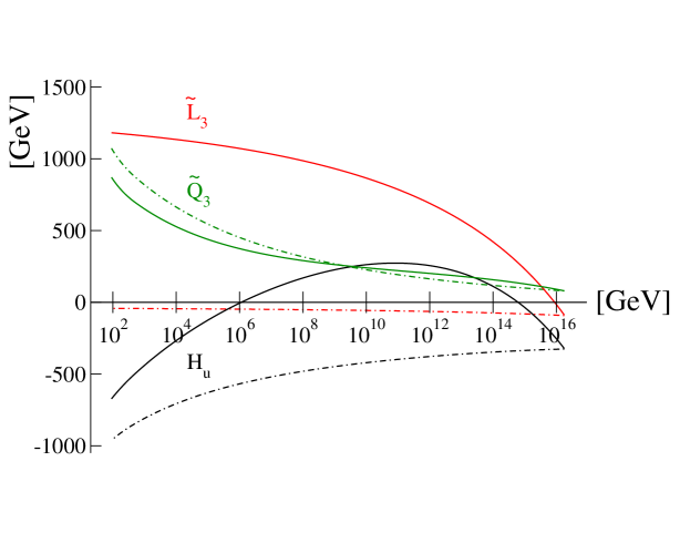
Figure 3.2: HCAMSB (solid) and pure AMSB (dotted) mass evolution from GUT scale to the weak scale for third-generation sleptons, third-generation squarks, and the up-type Higgs.

Pure hypercharge mediation however has the opposite effect on the third generation squarks. As we evolve to the weak scale, the left-handed stops may become tachyonic because they have relatively small hypercharge values and the same large Yukawa couplings of top quarks. But the stops also receive AMSB contributions that leave them with positive masses in the HCAMSB scenario. The anomaly and hypercharge mediation mechanisms are complementary in the respect that each helps to avoid the tachyonic particles that are present when only the other mechanism is present.
We can understand the extra suppression with increasing $\alpha$ for third generation squarks by taking a closer look at the RGEs. Both ${\tilde{t}}_{L}$ and ${\tilde{b}}_{L}$ belong to the same $SU(2)$ doublet, $Q_{3}$. The running of the doublet mass includes the terms [20]

$$\frac{dm_{Q_{3}}^{2}}{d(log\ Q)}\ni Y_{t}^{2}X_{t}+Y_{b}^{2}X_{b}$$ (3.14)

where $X_{t,b}$ is defined to be

$$X_{t} =m_{Q_{3}}^{2}+m_{{\tilde{t}}_{R}}^{2}+m_{H_{u}}^{2}+A_{t}^{2}$$ (3.15)

$$X_{b} =m_{Q_{3}}^{2}+m_{{\tilde{b}}_{R}}^{2}+m_{H_{d}}^{2}+A_{t}^{2}.$$ (3.16)

Again, right-handed particles have larger hypercharge than $SU(2)$ doublets, and the values $m_{{\tilde{t}}_{R}}^{2}$ and $m_{{\tilde{b}}_{R}}^{2}$ steepen the running slope near the weak scale. Then it is evident that for larger values of $\alpha$ in HCAMSB, the third generation doublet receives extra suppression from Yukawa effects relative to other generations. This suppression affects ${\tilde{t}}_{L}$- and ${\tilde{b}}_{L}$-production rates at the LHC for the HCAMSBmodel as will be discussed in the next section.
We can also see which RGE effect leads to $\mu$-suppression with increasing $\alpha$. The tree-level scalar minimization given by Equation 1.17 shows that $\mu$ goes as $-m_{H_{u}}^{2}$, and increasing $m_{H_{u}}^{2}$ implies decreasing $\mu$. The $m_{H_{u}}^{2}$ RGE includes the terms

$$\frac{dm_{H_{u}}^{2}}{d\ log(Q)}\ni-\frac{3}{5}g_{i}^{2}M_{i}^{2}+3Y_{t}^{2}X_{t}.$$ (3.17)

Again the large $M_{1}$ value uplifts $m_{H_{u}}^{2}$ in the early running from $Q=M_{GUT}$, and at low $Q$ Yukawa effects again dominate over the hypercharge effects. This is shown in Figures 3.2 and 3.3. In Figure 3.3 three values of $\alpha$ have been chosen and the 1-loop RGEs have been used in the evolution. As $\alpha$ increases the Higgs mass increases at the weak scale. For the largest $\alpha$ shown the Higgs mass is positive which could imply negative $\mu^{2}$ and therefore no electroweak symmetry breaking. However, when large 1-loop corrections are added to the scalar potential $\mu^{2}$ is once again positive. In Figure 3.3, $\alpha\sim 0.195$ is the upper edge of parameter space beyond which EW-breaking does not occur.

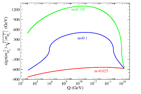
Figure 3.3: $m_{H_{u}}^{2}$ evolution for the three values of $\alpha$: 0.025, 0.01, and 0.195.

As already mentioned, $\mu$ is an important parameter in the neutralino sector. Towards higher values of $\alpha$, $\mu$ decreases as mentioned above and moves nearer to the value of $M_{2}$ (over all of the parameter space ${\tilde{Z}}_{1}$ is mainly wino and $M_{{\tilde{Z}}_{1}}\simeq M_{2}$). Here the ${\tilde{Z}}_{1}$ mass state is a mixture of wino and higgsino. Because of this, the mass splitting $\Delta M_{{\tilde{Z}}_{1}}$ between ${\tilde{W}}_{1}$ and ${\tilde{Z}}_{1}$ will increase leading to a shorter lifetime of the former.
To understand this last point, note that in the limit of $\mu$, $M_{1}>>M_{2}$ the mass eigenstates ${\tilde{Z}}_{1}$ and ${\tilde{W}}_{1}^{\pm}$ form an $SU(2)$ triplet with common mass $M_{2}$. The symmetry is broken by gaugino-higgsino mixing which leads to mass splitting between the neutralino and the chargino. As we saw in Chapter 2, $\Delta M_{{\tilde{Z}}_{1}}$ is important in the detection of charginos. We now see that the detection of the chargino can depend on the value of $\alpha$, and its lifetime is shown in Figure 3.4. As can be seen, larger $\alpha$ leads to shorter ${\tilde{W}}_{1}$ lifetimes.

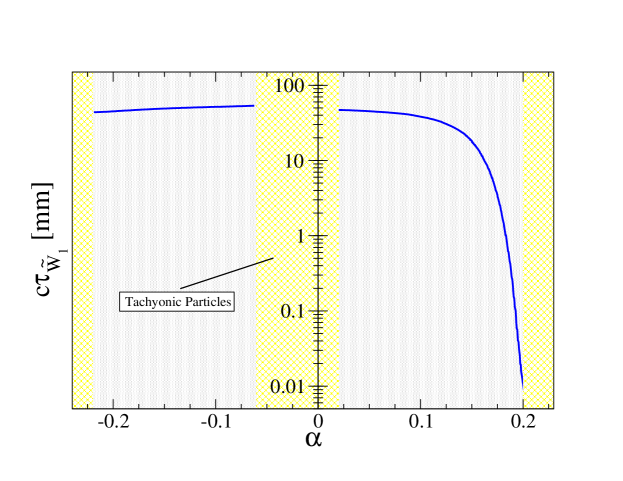
Figure 3.4: ${\tilde{W}}_{1}$ lifetime as a function of $\alpha$.

All of these results can be summarized as in Table 3.2 for the mAMSBpoint with $(m_{0},m_{3/2},\textrm{tan}\ \beta)$ = (300 GeV, 50 TeV, 10), and for similar parameter choices for two HCAMSBpoints, with a low and high value of $\alpha$, 0.025 and 0.195, defined respectively as points HCAMSB1 and HCAMSB2. By comparing the model lines we see that the table reflects all of the HCAMSBfeatures: L-R splitting, wino-like ${\tilde{Z}}_{1}$/${\tilde{W}}_{1}$, $m_{Q_{3}}$- and $\mu$-suppression and $\Delta M_{{\tilde{Z}}_{1}}$ increase with increasing $\alpha$, etc.

parameter	mAMSB	HCAMSB1	HCAMSB2
$\alpha$	—	0.025	0.195
$m_{0}$	300	—	—
$m_{3/2}$	$50\ {\rm TeV}$	$50\ {\rm TeV}$	$50\ {\rm TeV}$
$\tan\beta$	10	10	10
$M_{1}$	460.3	997.7	4710.5
$M_{2}$	140.0	139.5	137.5
$\mu$	872.8	841.8	178.8
$m_{{\tilde{g}}}$	1109.2	1107.6	1154.2
$m_{{\tilde{u}}_{L}}$	1078.2	1041.3	1199.1
$m_{{\tilde{u}}_{R}}$	1086.2	1160.3	2826.3
$m_{{\tilde{t}}_{1}}$	774.9	840.9	427.7
$m_{{\tilde{t}}_{2}}$	985.3	983.3	2332.5
$m_{{\tilde{b}}_{1}}$	944.4	902.6	409.0
$m_{{\tilde{b}}_{2}}$	1076.7	1065.7	1650.7
$m_{{\tilde{e}}_{L}}$	226.9	326.3	1973.1
$m_{{\tilde{e}}_{R}}$	204.6	732.3	3964.9
$m_{{\tilde{W}}_{2}}$	879.2	849.4	233.1
$m_{{\tilde{W}}_{1}}$	143.9	143.5	107.1
$m_{{\tilde{Z}}_{4}}$	878.7	993.7	4727.2
$m_{{\tilde{Z}}_{3}}$	875.3	845.5	228.7
$m_{{\tilde{Z}}_{2}}$	451.1	839.2	188.6
$m_{{\tilde{Z}}_{1}}$	143.7	143.3	105.0
$m_{A}$	878.1	879.6	1875.1
$m_{h}$	113.8	113.4	112.1

Table 3.2: Parameters and masses in GeV units for three case study points mAMSB, HCAMSB1 and HCAMSB2 using Isajet 7.79 with $m_{t}=172.6$ GeV and $\mu>0$.

3.4 HCAMSB Model Constraints

We now examine the allowed parameter space of the HCAMSBmodel and begin to infer some sparticle mass ranges observable at the LHC. There are both theoretical and experimental constraints for the model parameter space. On the theory side we have the requirement of proper electroweak symmetry breaking which implies that only $m_{H_{u}^{2}}$ can become less than zero because the scalar potential cannot be minimized by fields with conserved charges. If other mass parameters (including $\mu$) become negative and/or $H_{u}$ does not, then the corresponding region of parameter space is prohibited. Experimental constraints come in two varieties: direct and indirect. The direct constraints considered are the LEP2 mass limits on $m_{{\tilde{W}}_{1}}$ or $m_{h}$. Indirect constraints come from measurements that would be sensitive to supersymmetric particles appearing in loops. The indirect constraints considered here are the branching ratio from inclusive radiative B-meson decays, $BF(b\rightarrow s\gamma)$ [84], and $(g-2)_{\mu}$ measurements. Consideration of cosmological constraints are postponed until Chapter 5 where Dark Matter in AMSB models is discussed.

Figure 3.5: Allowed $m_{3/2}$-$\alpha$ parameter space for $\textrm{tan}\ \beta=10$ and $40$ with $\mu>0$ and $m_{t}=172.6$ GeV. The orange vertical lines at lower values of $m_{3/2}$ represent the LEP2 excluded region where $m_{{\tilde{W}}_{1}}<91.9$ GeV. The yellow regions at the far-right, far-left, and center are regions where electroweak symmetry is improperly broken. The white regions are acceptable, and constant-mass contours for ${\tilde{u}}_{1},{\tilde{g}},{\tilde{t}}_{1}$, and ${\tilde{e}}_{L}$ are shown.

We begin exploring the parameter space by plotting various masses in the $m_{3/2}-\alpha$ plane in Figure 3.5. The plots in the figure have excluded regions for improper EW symmetry breaking (yellow-thatched region) due to tachyonic sleptons at $\alpha\sim 0$ and $\mu^{2}<0$ at the extreme $\alpha$ values. The orange region at lower $m_{3/2}$ values is where $m_{{\tilde{W}}_{1}}$ is below the LEP2 limit of 91.9 GeV [80] in the search for nearly degenerate ${\tilde{W}}_{1}$s and ${\tilde{Z}}_{1}$s.
The plot shows that the region with $m_{3/2}\lesssim 30$ TeV are excluded by the LEP2 chargino limit. For $m_{3/2}\sim 30$ TeV, we have for the gluino $m_{\tilde{g}}\sim$ 730 GeV which is beyond the reach of any reasonable search at the Tevatron, so the discovery potential for this model must be investigated for the LHC. There is not an upper-bound on the gravitino mass, but the plot extends up to $m_{3/2}\sim$ 150 and 160 TeV for the 3 TeV contours in $m_{\tilde{g}}$ and $m_{{\tilde{u}}_{L}}$ respectively. These are somewhat above the reach of 2.1 TeV for squarks and 2.8 TeV for gluinos [30] predicted in the case of mAMSBfor the LHC. We will explore the reach of this model in Section 3.6.

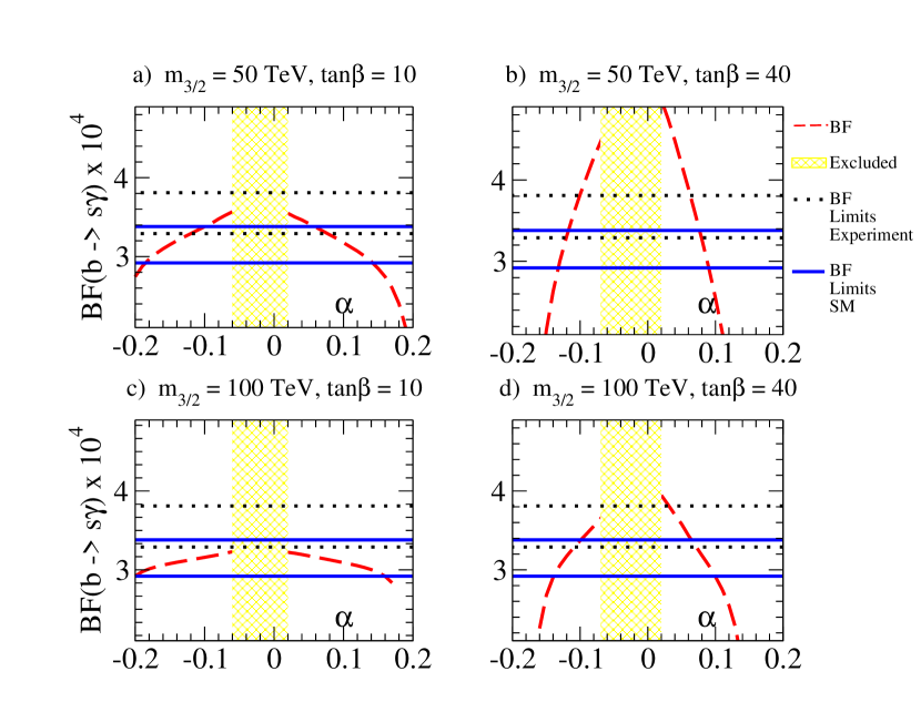
Figure 3.6: The branching fraction for $b\rightarrow s\gamma$ vs. $\alpha$ for combinations of $m_{3/2}=$ 50 and 100 TeV and $\textrm{tan}\ \beta=$ 10 and 40.

We also check whether there are regions of parameter space that agree with indirect measurements. Figure 3.6 shows the branching fraction of $b\rightarrow s\gamma$ as a function of $\alpha$ for four pairings of the $m_{3/2}$ and $\textrm{tan}\ \beta$ parameters to span the space. The dashed red line represent the HCAMSBvalues calculated with using the Isatools subroutine ISABSG [13]. The blue line is the theory result for the SM at order $\alpha_{s}^{2}$ [84] with the range of values $BF(b\rightarrow s\gamma)=3.15\pm 0.23\times 10^{-4}$. The black-dotted lines are the combined experimental branching fraction results of CLEO, BELLE, and BABAR [29] and have values in the range $BF(b\rightarrow s\gamma)=3.55\pm 0.26\times 10^{-4}$. The plot shows that there are regions of near-agreement in the parameter space of each case. Exceptions include the low $\alpha$ region in frame b) where the BF is too big, and very high $\alpha$ values in frames a), c), and d) where BF is too small. Finally, we close this section with contribution to $\frac{(g-2)_{\mu}}{2}$, denoted as $\Delta a_{\mu}^{SUSY}$, in the HCAMSBmodel. Figure 3.7 shows $\Delta a_{\mu}^{SUSY}$ calculated with ISAAMU from Isatools [17], with four plots with high and low values of $m_{3/2}$ and $\textrm{tan}\ \beta$. In each of the four cases, low $\alpha$ leads to relatively light ${\tilde{\mu}}_{L}$ and ${\tilde{\nu}}_{L}$ that appear in loop corrections to the photon vertex. This appears in the plots as larger corrections at low $\alpha$ to SM predictions. Parameter values with $\Delta a_{\mu}^{SUSY}\gtrsim 60\times 10^{-10}$ or $<0$ are disfavored [20].

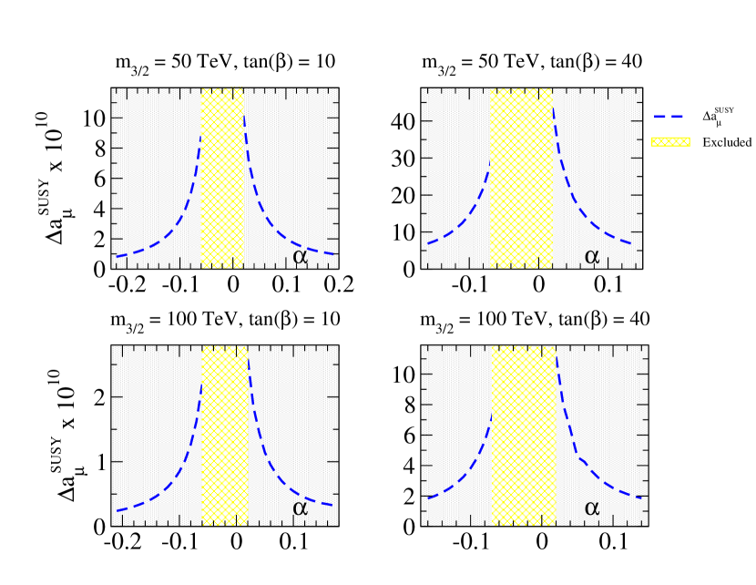
Figure 3.7: The SUSY contribution to $(g-2)_{\mu}$ as a function of $\alpha$.

3.5 HCAMSB Cascade Decays Patterns

All of the signatures at the LHC for the HCAMSB model will be shown in this section. That is, the physical outcome of those regions of parameter space that are not already excluded will be explored. We will also rely on the findings of section 3.3 to understand the production rates when necessary.
We begin by examining the largest LHC production cross sections in order to understand what are the HCAMSBsignatures. Note that all of the following analysis is done for the 14 TeV pp beams. Table 3.3 shows for the three model lines the total SUSY production cross section and the percentages for the pair-production for gluinos, squarks, EW-inos, sleptons, and light stops. It is seen that the EW-ino pairs dominate over all other production rates while squarks and gluinos are produced in lower, but still significant, amounts.
The dominant EW-ino cross sections come from the reactions $pp\rightarrow{\tilde{W}}_{1}^{+}{\tilde{W}}_{1}^{-}X$ and $pp\rightarrow{\tilde{W}}_{1}^{\pm}{\tilde{Z}}_{1}X$. However, the ${\tilde{W}}_{1}$ decays and the ${\tilde{Z}}_{1}$ do not lead to calorimeter signals that can serve as triggers for LHC detectors. So we must instead look at squark and gluino production mechanisms.

	mAMSB	HCAMSB1	HCAMSB2
$\sigma\ [{\rm fb}]$	$7.7\times 10^{3}$	$7.4\times 10^{3}$	$1.8\times 10^{4}$
${\tilde{g}},{\tilde{q}}\ pairs$	15.0%	15.5%	14.3%
$EW$-$ino\ pairs$	79.7%	81.9%	85%
$slep.\ pairs$	3.7%	0.8%	–
${\tilde{t}}_{1}{\tilde{\bar{t}}}_{1}$	0.4%	0.2%	5.5%
$BF({\tilde{Z}}_{2}\to{\tilde{Z}}_{1}Z)$	$0.01\%$	7.7%	22.3%

Table 3.3: HCAMSBrates for the LHC.

We first consider that $m_{3/2}$ = 30 TeV, the lowest value not excluded by experiment, and qualitatively discuss the emergence of the final states. Because of the absence of third-generation partons in the initial state, squark and gluino rates are determined by SUSY QCD and only depend on their respective masses. Since $m_{{\tilde{q}}_{L}}$, $m_{{\tilde{q}}_{R}}$ and $m_{\tilde{g}}$ have similar values for low $\alpha$, the final states ${\tilde{g}}{\tilde{g}},{\tilde{g}}{\tilde{q}}$, and ${\tilde{q}}{\tilde{q}}$ are produced at similar rates. In general, R-squarks are heavier than their L-partners due to the U(1) contribution. Already for low $\alpha$, $m_{{\tilde{u}}_{R}}$ and $m_{{\tilde{c}}_{R}}$ $>m_{\tilde{g}}$ (similarly to $m_{3/2}$ = 50 TeV in Figure 3.1). The subsequent decays of these squarks enhance the production of gluinos through ${\tilde{u}}_{R}\rightarrow u{\tilde{g}}$ and ${\tilde{c}}_{R}\rightarrow c{\tilde{g}}$. Gluinos finally decay in quark-squark pairs, and they have the highest rates into $b\bar{\tilde{b}}_{1}+h.c.$ and $t\bar{\tilde{t}}_{1}+h.c.$ and subdominant rates into other $q{\tilde{q}}_{L}$ pairs.
Conversely, as $\alpha$ increases, right-handed sparticle masses become larger to the point that eventually they cannot be produced in collisions. At higher values of $\alpha$, left-sparticles become heavier than ${\tilde{g}}$, while ${\tilde{t}}_{1}$ and ${\tilde{b}}_{1}$ are significantly lighter and again can be found in the main quark-squark decay modes of gluinos. At the highest $\alpha$ values, gluinos decay only into quark-squark pairs involving ${\tilde{t}}_{1}$s or ${\tilde{b}}_{1}$s: ${\tilde{g}}\rightarrow t{\tilde{t}}_{1}$ or $b{\tilde{b}}_{1}$.
We also find for high $\alpha$ that, in addition to ${\tilde{g}}\rightarrow{\tilde{t}}_{1}/{\tilde{b}}_{1}+X$, direct production of ${\tilde{b}}_{1}\bar{\tilde{b}}_{1}+h.c.$ and ${\tilde{t}}_{1}\bar{\tilde{t}}_{1}+h.c.$ pairs dominate over ${\tilde{g}}{\tilde{g}},{\tilde{g}}{\tilde{u}}_{L}$, and ${\tilde{g}}{\tilde{c}}_{L}$. The ${\tilde{t}}_{1}$ and ${\tilde{b}}_{1}$ mass eigenstates are mainly L-squarks at high $\alpha$, and appear approximately in a weak doublet. Thus they have nearly the same mass, $m_{{\tilde{t}}_{1}}\approx$ $m_{{\tilde{b}}_{1}}$, and their production rates are nearly identical. Figure 3.8 shows the direct production cross section of sbottom pairs using the program Prospino2.1 [33], and it is understood that pair-production cross section of stops is nearly equal.

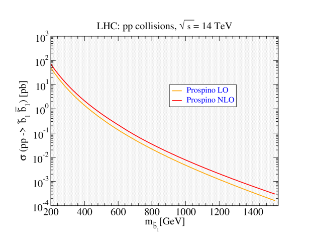
Figure 3.8: Total ${\tilde{b}}_{1}\bar{\tilde{b}}_{1}$ production cross section.

To recap the findings of the previous three paragraphs we see that light stop and sbottom squark, as well as top and bottom quarks are produced in the following ways:

low $\alpha$:	$\bullet$ gluino production and main decays to quark- squark pairs;
high $\alpha$:	$\bullet$ gluino production and subsequent decay purely to quark-squark pairs;
	$\bullet$ direct stop and sbottom pair production.

Obviously the production of stops and sbottoms is important in HCAMSBphenomenology. Then to proceed we need to examine the decay patterns of these particles to arrive at the final state.

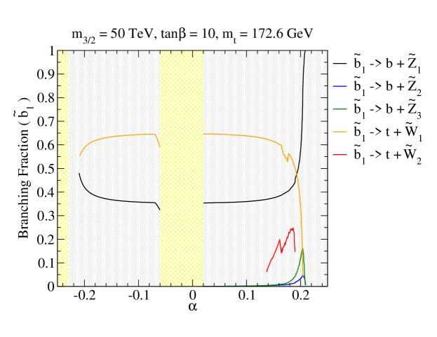
Figure 3.9: Branching fraction of ${\tilde{b}}_{1}$ for model parameters $m_{3/2}$ = 50 TeV, $\textrm{tan}\ \beta=10$, and $sgn(\mu)>0$.

Figure 3.10: Branching fraction of ${\tilde{t}}_{1}$ for model parameters $m_{3/2}$ = 50 TeV, $\textrm{tan}\ \beta=10$, and $sgn(\mu)>0$.

We now move from $m_{3/2}=$ 30 TeV up to 50 TeV to match the benchmark points and we find that the features of the previous paragraphs are unchanged. To proceed, the branching fractions of the lightest sbottoms and stops are plotted as a function of $\alpha$ in Figures 3.9 and 3.10. The features of low $\alpha$ are simple: both light sbottoms and stops decay to lightest charginos with about 67% and to lightest neutralinos with about 33%, and those make up the entire branching fractions. As $|\alpha|$ increases, $\mu$ decreases and approaches $M_{2}$, and again ${\tilde{Z}}_{1}$ makes the transition from wino-like to a wino-higgsino mix. ${\tilde{Z}}_{2}$ and ${\tilde{Z}}_{3}$ are mainly higgsino (as in Table 3.1) and become lighter with decreasing $\mu$, so that the decay channels ${\tilde{b}}_{1}\rightarrow b{\tilde{Z}}_{2},b{\tilde{Z}}_{3},t{\tilde{W}}_{2}$ and ${\tilde{t}}_{1}\rightarrow t{\tilde{Z}}_{2},t{\tilde{Z}}_{3},b{\tilde{W}}_{2}$ open. Finally, at the largest values of $|\alpha|$, the sbottoms and stops decrease in mass and the decay modes close. In particular, it can be seen in Figure 3.10 that all two-body modes for the light stop are closed, but its decays proceed via the ${\tilde{t}}_{1}\rightarrow bl\nu{\tilde{Z}}_{1}$ and $c{\tilde{Z}}_{1}$.
We also check what effects increasing $m_{3/2}$ has on the branching fractions. Figure 3.11 shows the branching fractions verses $m_{3/2}$ for sbottoms and stops at low $|\alpha|$. It is seen in both cases that out to very large values of $m_{3/2}$, two-body decays modes with ${\tilde{W}}_{1}$ and ${\tilde{Z}}_{1}$ are dominant while all others are subdominant. Explicitly, these modes are ${\tilde{t}}_{1}\rightarrow b{\tilde{W}}_{1},t{\tilde{Z}}_{1}$ and ${\tilde{b}}_{1}\rightarrow b{\tilde{Z}}_{1},t{\tilde{W}}_{1}$.

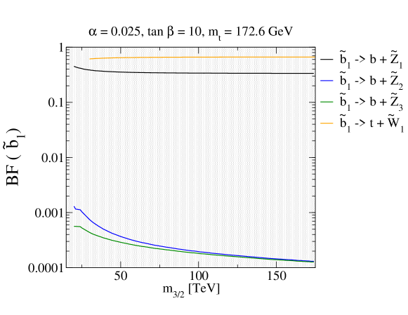
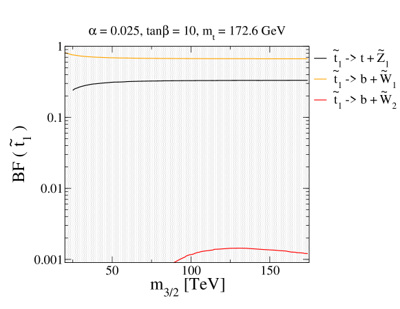
Figure 3.11: Branching fraction for ${\tilde{b}}_{1}$ (a) and ${\tilde{t}}_{1}$ (b) vs. $m_{3/2}$ for model parameters $\alpha=0.025$, $\textrm{tan}\ \beta=10$, and $sgn(\mu)>0$.

Then, to summarize the HCAMSBsignatures, we have seen that gluino and squark production always lead to cascade decays to third-generation quarks and squarks. From these products should emerge high multiplicities of $b-jets$ as well isolated leptons emerging from the $t\rightarrow bW$ decays. There should also be significant $\not{E}_{T}$ due to the presence of ${\tilde{Z}}_{1}$s and $\nu$s escaping the detectors. In addition to these, there is also the possibility of detecting highly-ionizing tracks as is usually for AMSB models. This is due to the wino-like nature ($M_{2}<<M_{1},\mu$) of ${\tilde{W}}_{1}$ and ${\tilde{Z}}_{1}$ states and to their near mass degeneracy that leads to a narrower width for the former. Because ${\tilde{W}}_{1}\rightarrow\pi^{+}{\tilde{Z}}_{1}$ has too soft a pion to leave a calorimeter signal (Chapter 2), the HITs should be seen to abruptly terminate without a calorimeter signal.

3.6 HCAMSB and the LHC

In this section we analyze events using the Isajet 7.79 [88] event generator (for specific details of the simulation, see section 1.5 of the Introduction). As we saw in section 3.4, the lowest gluino mass is too large to be detected at the Tevatron; we then must understand how HCAMSBwould appear at the LHC. It is expected that the LHC phenomenology will have similarities to mAMSB on general grounds. So part of the aim of this section will be to see in which ways this theory will be distinguishable from mAMSB at the LHC.
The discussion in this section is split into two subsections. In the first we flesh out the final states of cascade decays and optimize the cuts used to observe them. In the subsection that follows we analyze the reach for the LHC.

Final State Analysis

We generate 2M events for the points HCAMSB1 and HCAMSB2 from Table 3.2 and compare with SM backgrounds. QCD jets are generated with Isajet and include the following jet types: $g,u,d,s,c$, and $b$. Additional jets are produced in parton showering and other parton-level processes considered. Other backgrounds include the following: $W+jets$, $Z+jets$, $t\bar{t}$(172.6 GeV), and $WW,WZ$, and $ZZ$ vector boson production. Both $W+jets$ and $Z+jets$ have exact matrix elements for one parton emission and use parton showering for subsequent emissions.
We would like to apply cuts to these backgrounds without overly diminishing the signal (a “good” signal to be quantified in the next subsection on the LHC reach). Initially we choose the following cuts labeled C1:

• $n(jets)\geq 4$,

• $\not{E}_{T}>max$(100 GeV, 0.2 $M_{eff}$),

• ${E_{T}}(j_{1},j_{2},j_{3},j_{4})>$ 100, 50, 50, 50 GeV,

• Transverse sphericity: $S_{T}>0.2$,

where $M_{eff}=\not{E}_{T}+{E_{T}}(j_{1})+{E_{T}}(j_{2})+{E_{T}}(j_{3})+{E_{T}}(j_{4})$. After applying the C1 cuts we arrive at Figures 3.12 and 3.13. Figure 3.12 shows three multiplicity distributions: (a) number of jets, (b) number of b-jets, and (c) number of leptons. The kinematic distributions in Figure 3.13 are for (a) hardest jet $p_{T}$, (b) second hardest jet $p_{T}$, (c) $\not{E}_{T}$, and (d) the augmented effective mass, $A_{T}$ (this is the effective mass as earlier, but also includes $\sum{E_{T}}(leptons)$ and the ${E_{T}}$ of all jets). These distributions are used to improve on the cuts and each is discussed in the following.
Figure 3.12:

• (a) Jet multiplicity (after relaxing $n(jets)\geq 4$) after C1 cuts – signals for HCAMSBpoints 1 & 2 do not exceed background until very high jet multiplicities. For instance the HCAMSB1 distribution does not exceed background until $n(jet)\sim 9$. The selection of $n(jet)\geq 4$ should be beneficial in this case.

• (b) $b-jet$ multiplicity (after relaxing $n(jets)\geq 4$) after C1 cuts – signal cross section appears harder than background due to the appearance of extra $b$ and $t$ quarks from cascade decays as discussed in Section 3.5. The signals exceed background around $n(b-jet)\sim 5$. We conservatively choose events with at least a single $b-jet$ to cut down on background.

• (c) Lepton multiplicity after C1 cuts – we can see a much harder signal distribution of leptons than for background due to the presence of leptons from cascade decays as in the discussion of Section 3.5. The HCAMSB1 signal appears even stronger because sleptons are lighter at lower $\alpha$. Signal exceeds backgrounds around $n(l)\sim 3$, and HCAMSB1 has sufficient strength to be visible here with only a few fb^-1 of LHC data [22][21].

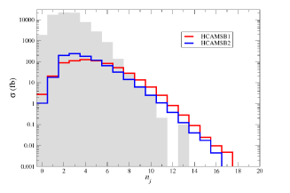
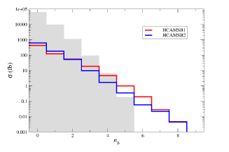
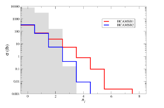
Figure 3.12: Jet, b-jet, and lepton multiplicity distributions for HCAMSBpoints 1 (red) & 2 (blue), and SM background (gray), all after C1 cuts.

Figure 3.13:

• (a) ${E_{T}}$ of hardest jet after C1 cuts (${E_{T}}(j_{1})$ cut relaxed) – the HCAMSB2 signal peaks for ${E_{T}}(jet_{1})\sim 150$ GeV because of ${\tilde{b}}_{1}\bar{\tilde{b}}_{1}$ production followed by ${\tilde{b}}_{1}\rightarrow b{\tilde{Z}}_{1}$. Signal exceeds background around 450 GeV for HCAMSB1 and 550 GeV for HCAMSB2.

• (b) ${E_{T}}$ of second hardest jet after C1 cuts (${E_{T}}(j_{2})$ cut relaxed) – Similar to (a), but signal exceeds background at ${E_{T}}(jet_{2})\sim$ 350 GeV for HCAMSB1 and $\sim$ 450 GeV for HCAMSB2.

• (c) $\not{E}_{T}$ after C1 cuts – the HCAMSB2 distribution is softer than for HCAMSB1 because the $\not{E}_{T}$ originates from third-generation squarks, $e.g.\ {\tilde{b}}_{1}\rightarrow b{\tilde{Z}}_{1}$, whereas in the latter case harder ${\tilde{Z}}_{1}$s are produced from TeV-scale squarks and gluinos.

• (d) Augmented effective mass – $A_{T}=$ $\not{E}_{T}+\sum{E_{T}}(jets)$ $+\sum{E_{T}}(isolated\ leptons)$. HCAMSB1 has a smooth distribution and exceeds background at $A_{T}\sim 1600$ GeV. The HCAMSB2 distribution interestingly has two components: a soft component with peak at $A_{T}\sim 750$ GeV due to third-generation squark pair production, and a hard component with peak at $A_{T}\sim 2000$ GeV due to ${\tilde{g}}$ and ${\tilde{q}}_{L}$ production.

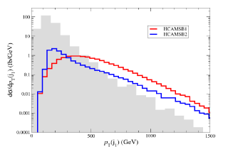
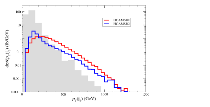
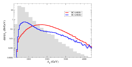
Figure 3.13: Kinematic distribution for HCAMSBpoints 1 (red) & 2 (blue) and SM background (gray) after C1 cuts.

And finally, in addition to the distributions just discussed, we consider Figure 3.14, which shows the oppositely-signed (OS), dilepton invariant mass distribution for HCAMSB points 1 & 2 and the background after C1 cuts and an extra cut of $A_{T}>1500$ GeV. This type of distribution is useful in SUSY studies because of the appearance of kinematic mass edges due to ${\tilde{Z}}_{2}\rightarrow{\tilde{l}}^{\pm}l^{\mp}$ or ${\tilde{Z}}_{2}\rightarrow\l^{\pm}l^{\mp}{\tilde{Z}}_{1}$ decays. For mAMSBmodels the bino-like ${\tilde{Z}}_{2}$ produce a mass edge since it efficiently decays to ${\tilde{l}}_{R}^{\pm}l^{\mp}$. In the HCAMSBmodel however, ${\tilde{Z}}_{2}$ is higgsino-like and rather heavy (see Table 3.1 for a comparison). In this case the decay channels are ${\tilde{Z}}_{2}\rightarrow{\tilde{W}}_{1}^{\pm}W^{\mp}$, ${\tilde{Z}}_{1}h$, and ${\tilde{Z}}_{1}Z$. Most importantly is the last decay channel which should always be open (except when $\mu\rightarrow 0$, when the $\alpha$ is at its very highest value) and occurs with a branching fraction at the tens of percent level. The decay to ${\tilde{Z}}_{1}Z$ of the bino-like ${\tilde{Z}}_{2}$ of mAMSBis highly suppressed due to the structure of $Z{\tilde{Z}}_{1}{\tilde{Z}}_{2}$ coupling [20], where Z couples to neutralinos only through their higgsino component. Thus we expect to be able to distinguish between HCAMSBand mAMSBmodels in the OS dilepton, invariant mass distribution because the former has a Z-peak structure and the latter does not. This is clear from Figure 3.14, which shows a clear Z-peak structure in HCAMSBpoints 1 & 2, and a diminished SM background.

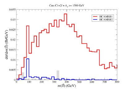
Figure 3.14: $m(l^{+}l^{-})$ distribution for HCAMSBpoints 1 (red) & 2 (blue) and SM background (gray) after C1 cuts.

LHC Reach

In this section we would like to understand the range of parameters accessible at the LHC. To this end, we vary over the range $m_{3/2}=30-200$ TeV and we adopt the two following model lines (again, low and high $\alpha$):

• HCAMSB1: $\alpha=0.025,\textrm{tan}\ \beta=10,\mu>0$,

• HCAMSB2: $\alpha=0.15,\textrm{tan}\ \beta=10,\mu>0$.

We take a somewhat lower value of $\alpha$ in HCAMSB2 than previously because $m_{3/2}$ could only be extended up to $\sim 60$ TeV before EW symmetry is improperly broken (see Figure 3.5). The spectrum is shown for the two points above while varying the $m_{3/2}$ parameter in Figure 3.15. The relative ordering of particle masses are unchanged.

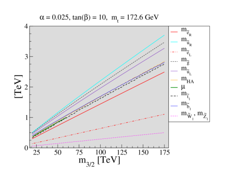
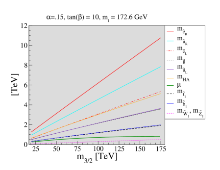
Figure 3.15: Spectrum versus $m_{3/2}$ for HCAMSBpoints 1 & 2.

The distributions of the last section allow us to improve on the background cuts. Instead of C1 cuts we will now use the following set of cuts that we label C2:

• $n(jets)\geq 2$,

• Transverse sphericity: $S_{T}>0.2$,

• $n(b-jets)\geq 1$,

• ${E_{T}}(j_{1}),{E_{T}}(j_{2}),\not{E}_{T}>E_{T}^{cut}$,

$E_{T}^{cut}$ will be variable minimum transverse energy value. Parameter space points with lower sparticle masses will benefit from a low $E_{T}^{cut}$, while points with high sparticle mass but lower production rates benefit from higher $E_{T}^{cut}$.
We apply the C2 cuts to the following lepton multiplicity channels: 0lep, 1lep, OS dilep, SS dilep, 3lep, and 4lep. As a supplement to the above cuts, in the 0lep channel, it is required that the $\not{E}_{T}$-(nearest jet ${E_{T}}$) transverse opening angle is constrained to $30^{\circ}<\Delta\phi(\not{E}_{T},{E_{T}}(j_{nearest}))<90^{\circ}$. Furthermore, all isolated leptons are required to have a minimum ${p_{T}}$ of 20 GeV, and events with single leptons are required to have transverse mass $M_{T}(l,\not{E}_{T})\geq 100GeV$ to reject leptons from W decays.

Process	$0\ell$	$1\ell$	$OS$	$SS$	$3\ell$
QCD($p_{T}$: 0.05-0.10 TeV)	–	–	–	–	–
QCD($p_{T}$: 0.10-0.20 TeV)	–	–	–	–	–
QCD($p_{T}$: 0.20-0.40 TeV)	73.5	–	–	–	–
QCD($p_{T}$: 0.40-1.00 TeV)	42.6	26.5	37.3	–	–
QCD($p_{T}$: 1.00-2.40 TeV)	0.8	0.6	0.3	0.015	–
$t\bar{t}$	1253.2	341.2	224.9	$0.25$	$0.25$
$W+jets;W\to e,\mu,\tau$	60.6	5.6	2.8	$--$	$--$
$Z+jets;Z\to\tau\bar{\tau},\ \nu s$	61.4	0.0	0.77	$--$	$--$
$WW,ZZ,WZ$	0.11	–	$--$	$--$	$--$
$Summed\ SM\ BG$	1492.3	374.1	266.1	$0.26$	$0.25$
HCAMSB1	100.1	53.2	13.1	2.4	3.3
HCAMSB2	223.5	58.7	4.6	1.7	0.35

Table 3.4: Estimated SM background cross sections (plus two HCAMSB benchmark points) in fb for various multi-lepton plus jets $+\not{E}_{T}$ topologies after cuts C2 with $E_{T}^{c}=100$ GeV.

The results of C2 cuts on SM background and the two model lines is shown in Table 3.4 for ${E_{T}^{c}}=100$ and for 2M events. Backgrounds cannot be detected for several multi-lepton channels. We consider an observable signal to be one that satisfies the following criteria for an assumed integrated luminosity:

• $S/B>0.2$,

• Signal has at least 5 events, and

• $S>5\sqrt{B}$,

Where $S$ and $B$ are the number of events for signal and background respectively. The first requirement is imposed to prevent the use of data that has a small signal on top of a large background, and that requires the use of extremely precise backgrounds [23]. The last requirement means that we require the signal to have a $5\sigma$ statistical significance above the background.
Using the criteria above and assuming 100 ${\textrm{fb}^{-1}}$ of data, we plot signal and background versus $m_{3/2}$ for C2 cuts with each of ${E_{T}^{c}}=100,300,$ and $500$ GeV and in each of the lepton multiplicity channels. Figure 3.16 shows the $5\sigma/5$ event SM background values with dotted horizontal lines, while the signal is represented by solid lines. Signal values above the horizontal lines qualify as observable. The value of $m_{3/2}$ where the solid line meets its corresponding (same color) dotted line is the value of $m_{3/2}$ that is accessible at the LHC. A SUSY signal is not observable where the solid line appears below the horizontal line.
The summary of the results from the plots in Figure 3.16 is given in Table 3.5. In the table, the upper entries are the $m_{3/2}$ reach values for point 1 ($\alpha=0.025$) and the lower entries are the same for point 2 ($\alpha=0.15$), and each row corresponds to a different ${E_{T}^{c}}$ value. The highest gravitino mass probed for ${E_{T}^{c}}=100$ GeV is 80 TeV and is found in the $3l$ channel. However, we can see by going to the harder cut, ${E_{T}^{c}}=500$ GeV, in the 0l channel, the reach is extended up to 115 TeV for $m_{3/2}$ for HCAMSB1. This value of $m_{3/2}$ corresponds to a gluino mass of $m_{\tilde{g}}\sim$ 2.4 TeV. Similarly, the best reach for HCAMSB2 is in the $0l$ channel with ${E_{T}^{c}}=500$ GeV, with the 105 TeV gravitino mass being probed, corresponding to a gluino mass of $\sim$ 2.2 TeV.

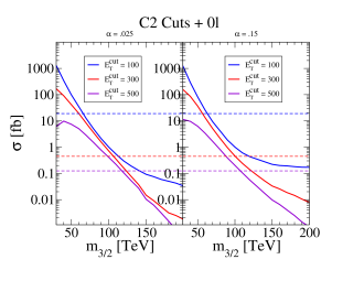
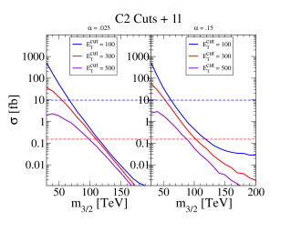
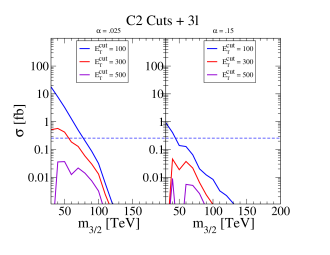
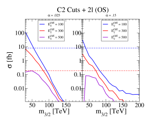
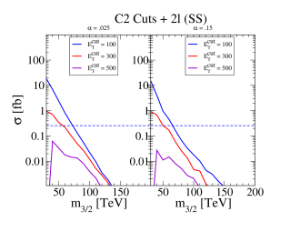
Figure 3.16: Cross section versus $m_{3/2}$ for HCAMSBpoints 1 & 2, after C2 cuts and in various lepton channels.

$E_{T}^{c}$ (GeV)	$0\ell$	$1\ell$	$OS$	$SS$	$3\ell$
100	$65/60$	$65/65$	$55/40$	$70/65$	$80/45$
300	$105/100$	$110/105$	$85/70$	$-/-$	$-/-$
500	$115/105$	$-/-$	$-/-$	$-/-$	$-/-$

Table 3.5: Estimated reach of 100 fb^-1 LHC for $m_{3/2}$ (TeV) in two HCAMSB model lines: $\alpha=0.025$ (upper entry) and $\alpha=0.15$ (lower entry), in various signal channels.

3.7 Summary

In this chapter we have given a complete analysis of the HCAMSBmodel relevant to physics at the LHC. We calculated the spectrum from which we were able to further calculate branching fractions and production cross sections, and to simulate LHC collider events for comparison again SM backgrounds. The final result of our analysis is that after 100 ${\textrm{fb}^{-1}}$ of data collection running at 14 TeV, the gravitino mass reach is $m_{3/2}\sim 115$ TeV ($m_{\tilde{g}}\sim 2.4$ TeV) for low values of $\alpha$, and $m_{3/2}\sim 105$ TeV ($m_{\tilde{g}}\sim 2.2$ TeV) for large $\alpha$. Since the spectra is so similar for $\mu>0$ and $\mu<0$, we do not expect changes in the reach due to the change in the $sgn(\mu)$. If instead $\textrm{tan}\ \beta$ was moved to higher values, we do not expect there to be differences in the $0l$ and $1l$ channels where we have maximal reach. Although it is possible there would be differences in the multi-lepton channels due to enhanced -ino decays to $\tau$s and $b$s at large $\textrm{tan}\ \beta$. In references [16][30], the mAMSBreach was shown to be around $m_{\tilde{g}}\sim 2.75$ TeV for low values of $m_{0}$, which is somewhat larger than for HCAMSB. This is due to the fact that squark masses tend to cluster around a common mass scale $m_{0}$ in mAMSB, while in the HCAMSBcase right and left squark states are highly split.
The mAMSBand HCAMSBmodels appear to have similar signatures at the LHC. Both would have multi-jet, multi-lepton, and $\not{E}_{T}$ events. In addition to these, long chargino tracks of $O(1-10)$ cm are possible. However, there are major differences between these two models that are summarized below.

• HCAMSBhas a highly left-right split scalar spectrum due to the left- right asymmetry in hypercharge assignments. For mAMSBthere is instead a near-equality between left and right mass parameters. The lightest stau, ${\tilde{\tau}}_{1}$, is mainly left-handed, while in mAMSBit is mainly right-handed. While it is possible that the left-right mixing could be determined at the LHC, this task would be easily done at a linear collider with polarized beams [15].

• We saw that high rate production of $b$s and $t$s was due to light ${\tilde{t}}_{1}$ and ${\tilde{b}}_{1}$ states relative to the gluino. In particular, with the HCAMSBmodel we expect high multiplicities of final state b-quarks, whereas for mAMSBmodels much few are expected (this also depends on the chosen $\textrm{tan}\ \beta$).

• We also see that the ordering of $\mu>M_{1}>M_{2}$ implied a bino-like ${\tilde{Z}}_{2}$ for mAMSB, while for HCAMSB, with $M_{1}>\mu>M_{2}$, it is higgsino-like. This crucially changes the decays of ${\tilde{Z}}_{2}$ and leads to an important distinction between mAMSBand HCAMSBmodels: the $m(ll)$ distribution for OS, dilepton events has a $Z\rightarrow l^{+}l^{-}$ peak in the latter, while the former would have a smooth distribution with no peak (except at large $\textrm{tan}\ \beta$ where there is greater mixing in the neutralino sector). Thus, HITs (see Chapter 2) from charginos and a Z-peak from ${\tilde{Z}}_{2}$ decays could yield a promising signal for HCAMSBand LHC.

4 inoAMSB

4.1 Introduction to inoAMSB Models

The combination of anomaly mediated (Section 1.4) and gaugino mediated [67] soft SUSY breaking parameters is suggested by two classes of models that arise in type IIB string theories compactified on a Calabi-Yao Orientifold (CYO). These model types differ in the number of Kähler moduli and they are:

• Single Kähler modulus (SKM models) – KKLT type with uplift of soft terms and cosmological constant coming from one-loop effects, and generally favors smaller CY compactification volumes;

• Large Volume Scenario (LVS models) – require at least two moduli and, as the name implies, favors larger CY compactification volumes.

The F-terms of moduli are responsible for SUSY breaking. In both cases the moduli are stabilized using a combination of fluxes and non-perturbative effects while the interactions with the MSSM are gravitational. The models also share two crucial features: gauginos receive their masses only from Weyl anomalies (string contributions are suppressed) and the soft scalar and trilinear parameters are naturally suppressed as usual in gaugino mediated scenarios (see [67][20]).
Having just analyzed the HCAMSBmodel, it should be possible to study other models in a similar fashion. In this chapter we do just that for a class of string models whose soft parameters arise in a pattern that we call the “Gaugino Anomaly Mediated SUSY Breaking” pattern, or more succinctly, “inoAMSB” [26]. The string theory origin for this model is quite different than for the case of HCAMSB, but we will see some similarities in the spectra that will lead to collider signatures already familiar from the last chapter. Furthermore, we will more or less follow the same procedure for arriving at the collider analysis level. Schematically this procedure is as follows:

• define the model high-scale boundary conditions,

• discuss the evolution of theory parameters from high-scale to TeV scale,

• explore the allowed parameter space subject to experimental constraints,

• choose the generally representative points for collider analysis and examine branching fractions and cross sections to determine possible signatures,

• and finally, determine the parameter reach for an experiment to produce a statistically significant signal.

4.2 Setup of the inoAMSBModels

Before moving on to the details of the models we should first consider a few preliminaries. A supergravity model is defined in terms of three functions: a superpotential, a Kähler potential, and the gauge kinetic function. They each have implicit $\Phi$ dependence and can be expanded in a series of MSSMsuperfields ($C^{\alpha}$) as follows:

$$W =\hat{W}(\Phi)+\mu(\Phi)H_{d}H_{u}+\frac{1}{6}Y_{\alpha\beta\gamma}C^{\alpha}C^{\beta}C^{\gamma}+\dots$$ (4.1)

$$K =\hat{K}(\Phi,\bar{\Phi})+\tilde{K}_{\alpha\beta}(\Phi,\bar{\Phi})C^{\alpha}C^{\beta}+[Z(\Phi,\bar{\Phi})H_{d}H_{u}+h.c.]+\dots,$$ (4.2)

$$f_{a} =f_{a}(\Phi).$$ (4.3)

The role of these moduli fields is to break supersymmetry. This happens once they are stabilized and acquire VEVs such that at least one of them has a non-zero F-term.
Each of the first terms in the above expansions have implicit dependence on the Calabi-Yau Orientifold (CYO):

$$\hat{K} =-2\rm{ln}({\cal V}+\frac{\xi}{2})-ln(i\int\Omega\wedge\bar{\Omega}(U,\bar{U}))-ln(S+\bar{S}),$$ (4.4)

$$\hat{W} =\int G_{3}\wedge\Omega+\sum_{i}A_{a}e^{-a_{i}T^{i}}.$$ (4.5)

Most notably, the first term in $\hat{K}$ contains the CYO volume, $\cal V$, and a stringy correction $\hat{\xi}$ that depends on the Euler character of the CYO and the real part of the dilaton superfield S. The last term in $\hat{W}$ is non-perturbative and is responsible for stabilizing the Kähler modulus at the minimum of the potential as in KKLT models. $\Omega$ are 3-forms on the CYO and are functions of $U_{r}$, the complex structure moduli.
The standard SUGRA potential is given by

$$V(\Phi)=F^{A}F^{\bar{B}}K_{A\bar{B}}-3|m_{3/2}(\Phi)|^{2},$$ (4.6)

where the SUSY breaking F-terms at the minimum are given by $F^{A}=e^{K/2}K^{A\bar{B}}D_{\bar{B}}W$, and the covariant derivatives are given by $D_{A}=\partial_{A}+K_{A}$, where subscripts indicate derivatives with respect to fields. Also, $\Phi$ stands collectively for all moduli that describe the internal geometry of the CYO plus the axion-dilaton. The minimum of the potential, $V_{0}$, gives the cosmological constant (CC) of the theory. The CC is known to be small, and taking it to be close to zero implies that at the minimum of the potential $F^{A}\stackrel{{\scriptstyle<}}{{\sim}}m_{3/2}$.

Single Kähler Modulus Scenario (SKM)

This model has IIB string theory compactified on a CYO, has only one Kähler modulus, T, and the MSSMfields come from open string fluctuations on a stack of D3 branes. Other moduli and the axio-dilaton are stabilized by internal fluxes and non-perturbative effects, as in KKLT .
At the classical level the CC would be small in magnitude but negative and the soft masses would be highly suppressed. However, because SUGRA theories have quadratic divergences at the quantum level (unlike broken global SUSY ), there are corrections to these quantities that are dependent on the string scale cutoff $\Lambda$. Such contributions can serve to uplift the CC to small and positive values and can generate soft SUSY breaking masses proportional to $\frac{\Lambda}{4\pi}m_{3/2}$. The cutoff is taken to be the string scale and can be between $\sim 10^{14}$ GeV and $\sim M_{GUT}$.

Large Volume Scenario (LVS)

In this class of models [28], IIB string theory is again compactified on a CYO. However, now more than one Kähler modulus is considered, $T_{i}$ $(i=1,\dots,h_{11}$). In particular, in the simplest situation there is a large modulus, $\tau_{b}$, and small moduli, ($\tau_{s}$ , $\tau_{a}$), controlling the overall size of the CYO and the volume of two small 4-cycles respectively. The total volume is then given by

$${\cal V} =\tau_{b}^{3/2}-\tau_{s}^{3/2}-\tau_{a}^{3/2}.$$ (4.7)

This is referred to as a “Swiss Cheese” model. Again the MSSM may be located on D3 branes at a singularity. Alternatively, it could be placed on a stack of D7 branes wrapping a four cycle (taken to be the one labelled by the index “a”). In this case, it has been argued [35] that the necessity of having chiral fermions on this brane prevents this cycle from being stabilized by non-perturbative effects and it shrinks below the string scale. Effectively, this means that the physics is the same as in the D3 brane case.
Extremizing the potential leads to an exponentially large volume [28] $V\sim e^{a\tau_{s}},\tau_{s}\sim\hat{\xi}$. It turns out that the suppression of FCNC effects lead to $V\sim 10^{5}l_{P}$ [47] (where $l_{P}$ is the Planck length), so the string scale is $M_{string}\sim M_{P}/\sqrt{V}\sim 10^{15.5}$ GeV. The minimum of the potential (CC) is given by $V_{0}\sim-\frac{m_{3/2}^{2}M_{P}^{2}}{\ln m_{3/2}\mathcal{V}}$. This minimum can be uplifted to zero when $S$ and $U_{r}$ acquire (squared) $F$-terms of the order $\frac{m_{3/2}^{2}M_{P}^{2}}{\ln m_{3/2}\mathcal{V}}$. Classical contributions to the scalar and slepton masses are also of this same order. With the above lower bound on the volume, this means that even for $m_{3/2}\sim 100$ TeV, the classical soft terms are $\stackrel{{\scriptstyle<}}{{\sim}}100$ GeV. Of course if one wants to avoid fine-tuning of the flux superpotential, it would be necessary to take even larger values of ${\cal V}$ corresponding to a string scale of $10^{12}$ GeV. In this case the classical soft terms are completely negligible (for $m_{3/2}\sim 100$ TeV) but the (classical) $\mu$-term is also strongly suppressed.
In the rest of this section the holomorphic variable associated with the large modulus $\tau_{b}$ will be called $T$.

Gaugino Masses - Weyl Anomaly Effects

For a generic version of supergravity, the gaugino masses satisfy the following relation at the classical level:

$$\frac{M_{a}}{g_{a}^{2}}=\frac{1}{2}F^{A}\partial_{A}f_{a}(\Phi).$$ (4.8)

In the single Kähler modulus model the MSSM resides on D3 branes at a singularity. In the LVS case, we may either have the MSSM on D3 branes at a singularity, or we may have it on a stack of D7 branes wrapping a four cycle which shrinks below the string scale. In both cases the classical gauge coupling function is effectively of the form

$$f_{a}=S$$ (4.9)

where $S$ is the axio-dilaton (for more details see [47] section 3.1 and references therein). The important point is that it is independent of the modulus $T$. So at a classical minimum, where the SUSY breaking is expected to be in the $T$ modulus direction, the string theoretic contribution to the gaugino mass is highly suppressed.
However, there is an additional contribution to the gaugino mass due to the (super) Weyl anomaly as discussed in Section 1.4. This comes from the expression for the effective gauge coupling superfield that has been derived by Kaplunovsky and Louis [68] (KL). For the gaugino masses, the relevant contribution comes from taking the $F$-term of

$$H_{a}(\Phi,\tau,\tau_{Z})=f_{a}(\Phi)-\frac{3c_{a}}{8\pi^{2}}{\rm ln}C-\frac{T_{a}(r)}{4\pi^{2}}\tau_{Z}.$$ (1.37)

Here, the first term on the RHS is the classical term; the second comes from the anomaly associated with rotating to the Einstein-Kähler frame. $c_{a}=T(G_{a})-\sum_{r}T_{a}(r)$ is the anomaly coefficient and the last term comes from the anomaly associated with the transformation to canonical kinetic terms for the MSSM fields. Also note that we have ignored the gauge kinetic term normalization anomaly [9, 46] which is a higher order effect. The chiral superfields $\phi,\phi_{r}$ that generate these transformations are given by,

$${\rm ln}C+{\rm ln}\bar{C} = \frac{1}{3}K|_{\rm harmonic},$$ (4.10)

$$\tau_{Z}+\bar{\tau}_{Z} = \ln\det\tilde{K}_{\alpha\bar{\beta}}^{(r)}.$$ (4.11)

The instruction on the RHS of the first equation is to take the sum of the chiral and anti-chiral (i.e. harmonic) part of the expression. After projecting the appropriate $F$ terms we arrive at the following expression:

$$\frac{2M_{a}}{g_{a}^{2}}=F^{A}\partial_{A}f_{a}-\frac{c_{i}}{8\pi^{2}}F^{A}K_{A}-\sum_{r}\frac{T_{i}(r)}{4\pi^{2}}F^{A}\partial_{A}\ln\det\tilde{K}_{\alpha\bar{\beta}}^{(r)}.$$ (4.12)

The first (classical) term is greatly suppressed relative to $m_{3/2}$ since the $T$-modulus does not contribute to the classical gauge coupling function as discussed earlier (see paragraph after (4.8)). The dominant contribution therefore comes from the last two (Weyl anomaly) contributions. It turns out that (after using the formulae $F^{T}=-(T+\bar{T})m_{3/2}$, $K_{T}=-3/(T+\bar{T})$ and $\tilde{K}_{\alpha\bar{\beta}}=k_{\alpha\beta}/(T+\bar{T})$ which are valid up to volume suppressed corrections), this yields,

$$M_{a}=\frac{b_{a}g_{a}^{2}}{16\pi^{2}}m_{3/2},$$ (4.13)

where $b_{a}=-3T(G_{a})+\sum_{r}T_{a}(r)$ is the beta function coefficient.

Scalar Masses, Trilinear Couplings, $\mu$ and $B\mu$ terms

Here are summarized the results from this class of string theory models for the values of the soft parameters at the UV scale, i.e. $\Lambda\sim M_{string}\sim M_{P}/\sqrt{{\cal V}}$. These values should be the initial conditions for the RG evolution of these parameters. In the LVS case, it was estimated [47] that the lower bound on the CYO volume was ${\cal V}>10^{5}$. Also, typical values of $h_{21}\sim O(10^{2})$ are chosen for the number of complex structure moduli. The gravitino mass is chosen to be $m_{3/2}\sim|W|M_{P}/{\cal V}\sim 50\ {\rm TeV}$. Such a large value of $m_{3/2}$ allows us to avoid the SUGRA gravitino problem, which leads to a disruption of Big Bang nucleosynthesis if $m_{3/2}\stackrel{{\scriptstyle<}}{{\sim}}5$ TeV and $T_{R}\stackrel{{\scriptstyle>}}{{\sim}}10^{5}$ GeV [74][77][91].
Unlike the gaugino masses, scalar masses and trilinear soft terms do not acquire corrections from the Weyl anomaly. They are essentially given at the UV scale by their classical string theory value plus one loop string/effective field theory corrections. In the $h_{11}=1$ case, the classical soft terms are essentially zero while in the LVS case

$$m_{0}\sim O\left(\frac{m_{3/2}}{\sqrt{\ln m_{3/2}{\cal V}}}\right),\ \ \mu\sim\frac{B\mu}{\mu}\stackrel{{\scriptstyle<}}{{\sim}}\sqrt{h_{21}}m_{0},\ \ A_{0}\ll m_{0}.$$ (4.14)

As discussed in [47] the estimate of the $\mu,B\mu$ term comes from the generic case of assuming that the uplift of the negative CC is distributed amongst the complex structure moduli as well as the dilaton. It was estimated in that reference that the $F$-term for a complex structure modulus is $|F_{m}|\stackrel{{\scriptstyle<}}{{\sim}}m_{3/2}/\sqrt{h_{21}(\ln m_{3/2})\cal{V}}$. Since the expression for the $\mu$ term involves a sum over $h_{21}$ terms this gives the estimate in (4.14). The parametric dependence on the volume factor in the upper bounds for the $\mu,B\mu/\mu$ terms goes as $\sqrt{h_{21}}/\sqrt{\cal V}$ and clearly favors the “small” values CYO volume i.e. ${\cal V}\sim 10^{5}$ and the large values of the number of complex structure moduli ($\sim 10^{2}$). However it should be stressed that these estimates are on a different footing than the rigorous calculation of $m_{0}$ and the gaugino masses, and indeed it is possible that these LVS models may have a $\mu$-problem.
After adding quantum corrections at the UV scale, both cases give similar values for the soft terms. As an example, this is illustrated for two values for the CYO volume:

• ${\cal V}\sim 10^{5},M_{string}\sim\Lambda\sim 10^{-2.5}M_{P}\sim 10^{15.5}\ {\rm GeV}$. Then,

  $$\mu\sim\frac{B\mu}{\mu}\stackrel{{\scriptstyle<}}{{\sim}}250\ {\rm GeV},\,m_{0}\sim 25\ {\rm GeV},\,A_{0}\ll m_{0}.$$ (4.15)

• ${\cal V}\sim 10^{12},\ M_{string}\sim\Lambda\sim 10^{-6}M_{P}\sim 10^{12}\ {\rm GeV}$. Then,

  $$\mu\sim\frac{B\mu}{\mu}\stackrel{{\scriptstyle<}}{{\sim}}10^{-1}\ {\rm GeV},\,m_{0}\sim 10^{-2}\ {\rm GeV},\,A_{0}\ll m_{0}.$$ (4.16)

The second very large volume case can be accessed only in the LVS model. Our favored case however is the first one with a volume around ${\cal V}\sim 10^{5}$ in Planck units. It should be noted that even with this value, it is only expected that stringy corrections to the numerical estimates of the above values of the soft masses etc. will be of order $\alpha^{\prime}/R_{CYO}^{2}\sim 1/{\cal{V}}^{1/3}\stackrel{{\scriptstyle<}}{{\sim}}10\%$.
The first case is at the lower bound for the volume. This gives the largest allowable string scale. This is still somewhat below the apparent unification scale, but it is close enough that (allowing for undetermined $O(1)$ factors) the GUT scale may be used as the point at which to impose the boundary conditions. This is useful for the purpose of comparing with other models of SUSY mediation where it is conventional to use the GUT scale.
The second case above corresponds to choosing generic values of the flux superpotential, while the first needs a fine tuned set of fluxes to get $|W|\sim 10^{-8}$, in order to have a gravitino mass of $\sim 10^{2}$ TeV, though in type IIB string theory general arguments show that there exist a large number of solutions which allow this. The most significant problem with the second case (apart from the fact that there is no hope of getting a GUT scenario) is the extremely low upper bound on the $\mu$ term. In other words, there is a serious $\mu$- problem. The first case also may have a $\mu$ term problem, but again since these estimates are accurate only to $O(1)$ numbers, it is possible to envisage that the problem can be resolved within the context of this model.
In any case, the string theory input is used to suggest a class of phenomenological models. Given that in both the GUT scale model and the intermediate scale model, the soft scalar mass and $A$ term are suppressed well below the weak scale and assumed to be zero for these at the UV scale, while the gaugino masses at this scale are given by

$$M_{a}=\frac{b_{a}g_{a}^{2}}{16\pi^{2}}m_{3/2}$$ (4.17)

as was the case in the last subsection.
The case when the input scalar mass $m_{0}$ is non-negligible will also be discussed. This would be the case for instance in the SKM model with smaller volumes and/or larger values of $h_{21}$, and also in the case of LVS with the volume at the lower bound but with larger values of $h_{21}$.

4.3 Spectrum, Parameter Space, and Constraints

The parameter space for this model is

$m_{3/2},\textrm{tan}\ \beta$, and $sgn(\mu)$,

and, given the discussion of the previous section the boundary conditions

$$m_{0}=A_{0}=0$$ (4.18)

are imposed along with AMSB masses for gauginos at $M_{string/GUT}$. Note that even when $m_{0}$ and $A_{0}$ are negligible at the GUT, scalars will be massive at the weak scale due to uplift from gauginos in the renormalization group running.
To illustrate the running of soft masses from the GUT scale to the weak scale, Figure 4.1 shows gaugino masses (top) and scalars (bottom) for the point $m_{3/2}$ = 50 TeV, $\textrm{tan}\ \beta=10$, and $\mu>0$ for $M_{\rm{string}}=M_{GUT}$. Gauginos begin with the usual ratio of ($M_{1}:M_{2}:M_{3}$) = (6.6 : 1 : -4.5), but at the weak scale the 1 and 3 masses switch in ordering leaving $|M_{3}|>>M_{1}>M_{2}$. The lower value of $M_{2}$ indicates that the lightest neutralino will be wino-like. Scalars begin with negligible masses as required by the boundary conditions. However the mass parameters are uplifted by radiative self-couplings. In particular, the large value of $M_{1}$ is responsible for the uplift near the $M_{GUT}$. In the early running the right-slepton, $E_{3}$, moves to the highest values because it has the largest hypercharge ($Y$=2). Because the hypercharges for the left-sleptons are lower than for the right-sleptons, they appear to have lower masses at the weak scale, which leaves us with a left-right split spectrum for sleptons. This effect is similar to what was seen in the case of HCAMSB, although the splitting for that model was more severe because of the much heavier $M_{1}$. Squarks receive extra uplift from QCD effects leaving them in the TeV range, while sleptons are generally lower: approximately between 200-400 GeV. Also, since ${\tilde{Z}}_{1}$ is wino-like and $M_{2}<\sqrt{m_{{\tilde{L}}_{3}}^{2}}$, charged LSPs are not of concern.

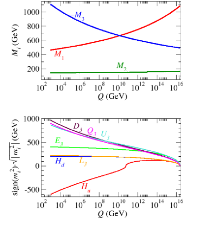
Figure 4.1: inoAMSB soft SUSY breaking parameters as a function of energy scale Q for model parameters $m_{3/2}$=50 TeV, $\textrm{tan}\ \beta$=10, $\mu>0$, and $M_{\rm{string}}$=$M_{GUT}$.

At the weak scale, physical masses and mixings are computed as usual and 1-loop corrections are added. The resulting spectrum for two inoAMSBpoints with $m_{3/2}$ = 50 and 100 TeV is listed in columns 3 and 4 of Table 4.1. In column 1 of the same table is the mAMSBpoint with $m_{0}=300$ GeV in column 2 is an HCAMSBpoint with $\alpha=0.025$ for comparison. By inspection it is seen that the features of the previous paragraph are represented in the table: large left-right splitting of sleptons, generally heavier squarks, and a ${\tilde{Z}}_{1}$ with a mass close to $M_{2}$ reflecting that it is wino-like. By comparison, HCAMSBhas a much larger left-right splitting in the sleptons (reflective of the heavier $M_{1}$ in that case), whereas mAMSBhas a much smaller splitting (nearly-degenerate with $m_{{\tilde{e}}_{R}}<m_{{\tilde{e}}_{L}}$).

parameter	mAMSB	HCAMSB1	inoAMSB1	inoAMSB2
$\alpha$	—	0.025	—	—
$m_{0}$	300	—	—	—
$m_{3/2}$	$50\ {\rm TeV}$	$50\ {\rm TeV}$	$50\ {\rm TeV}$	$100\ {\rm TeV}$
$\tan\beta$	10	10	10	10
$M_{1}$	460.3	997.7	465.5	956.1
$M_{2}$	140.0	139.5	143.8	287.9
$\mu$	872.8	841.8	607.8	1127.5
$mg$	1109.2	1107.6	1151.0	2186.1
$m_{{\tilde{u}}_{L}}$	1078.2	1041.3	1011.7	1908.7
$m_{{\tilde{u}}_{R}}$	1086.2	1160.3	1045.1	1975.7
$m_{{\tilde{t}}_{1}}$	774.9	840.9	878.8	1691.8
$m_{{\tilde{t}}_{2}}$	985.3	983.3	988.4	1814.8
$m_{{\tilde{b}}_{1}}$	944.4	902.6	943.9	1779.5
$m_{{\tilde{b}}_{2}}$	1076.7	1065.7	1013.7	1908.3
$m_{{\tilde{e}}_{L}}$	226.9	326.3	233.7	457.8
$m_{{\tilde{e}}_{R}}$	204.6	732.3	408.6	809.5
$m_{{\tilde{W}}_{2}}$	879.2	849.4	621.2	1129.8
$m_{{\tilde{W}}_{1}}$	143.9	143.5	145.4	299.7
$m_{{\tilde{Z}}_{4}}$	878.7	993.7	624.7	1143.2
$m_{{\tilde{Z}}_{3}}$	875.3	845.5	614.4	1135.8
$m_{{\tilde{Z}}_{2}}$	451.1	839.2	452.6	936.8
$m_{{\tilde{Z}}_{1}}$	143.7	143.3	145.1	299.4
$m_{A}$	878.1	879.6	642.9	1208.9
$m_{h}$	113.8	113.4	112.0	116.0

Table 4.1: Masses and parameters in GeV units for four case study points mAMSB1, HCAMSB1, inoAMSB1 and inoAMSB2 using Isajet 7.80 with $m_{t}=172.6$ GeV and $\mu>0$. Also listed are the total tree level sparticle production cross section in fb at the LHC.

The inoAMSBparameter space is simpler than either the mAMSBor HCAMSBcase because it has one less model parameter. We begin by recognizing that once a point is chosen, the increasing $m_{3/2}$ value increases all masses but leaves the relative hierarchy unchanged. This is demonstrated in Figure 4.2 (a) where the spectrum is plotted versus $m_{3/2}$ for $\textrm{tan}\ \beta=10$ and $\mu>0$. Everywhere in the parameter space of the inoAMSBmodel the hierarchy is generally in the order $m_{\tilde{g}}>m_{\tilde{q}}$ $>|\mu|$ $>m_{{\tilde{e}}_{R}}$ $>m_{{\tilde{e}}_{L},{\tilde{\nu}}_{L}}$ $>m_{{\tilde{Z}}_{1},{\tilde{W}}_{1}}$. We then expect squark pairs to be produced in LHC events either directly or through the decay of pair-produced gluinos. Furthermore, because squarks are heavier than sleptons we can expect squark cascade decays to two hard jets + isolated leptons through ${\tilde{q}}\rightarrow$ $q{\tilde{Z}}_{i}\rightarrow$ $q{\tilde{l}}^{\pm}l^{\mp}$.
In frame (b) of Figure 4.2, taking $m_{3/2}$ = 50 TeV, an example of the spectrum versus $\textrm{tan}\ \beta$ is given. Some interesting effects occur in the region of high $\textrm{tan}\ \beta$. There are noticeable dips in the masses for ${\tilde{b}}$ and ${\tilde{\tau}}$ eigenstates since larger $\textrm{tan}\ \beta$ results in larger Yukawa couplings for these particles, and thus greater suppression of masses when approaching the TeV scale. The $m_{A}$ parameter decreases most significantly in the plot. Because of the increased down-type Yukawa couplings for large $\textrm{tan}\ \beta$, $m_{H_{d}}$ is pushed towards negative values. Since the EW-breaking minimization conditions give $m_{A}^{2}\sim m_{H_{d}}^{2}-m_{H_{u}}^{2}$, the pseudoscalar too decreases for larger $\textrm{tan}\ \beta$. Negative values of $m_{H_{d}}^{2}$ signal improper breaking and this occurs around $\textrm{tan}\ \beta\sim 42$. And finally, $m_{A}$ cannot fall below the LEP2 bounds on the Higgs. In the plot $m_{h}\sim 111$ GeV which we consider near the acceptable edge due to the $\pm 3$ GeV error in the theory calculation. As $\textrm{tan}\ \beta$ increases, the LEP2 bound is violated, and shortly thereafter the EW symmetry is not properly broken. It can also been seen that at the lowest $\textrm{tan}\ \beta$ values, the lightest Higgs is too light.

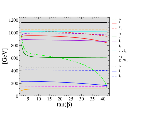
Figure 4.2: Sparticle masses: (a) as function of $m_{3/2}$, with $\textrm{tan}\ \beta=10$, $\mu>0$, and $M_{\rm{string}}=M_{GUT}$; (b) as a function of $\textrm{tan}\ \beta$, with $m_{3/2}=$ 50 TeV, $\mu>0$, and $M_{\rm{string}}=M_{GUT}$.

With the features of Figure 4.2 in mind, we look at the entire $\textrm{tan}\ \beta-m_{3/2}$ parameter space in Figure 4.3. The orange region is specifically excluded by LEP2 bounds on the chargino mass, and all $m_{3/2}$ values between this region and zero are likewise excluded. The brown regions are also excluded as in Figure 4.2 (b): the high $\textrm{tan}\ \beta$ regions has improper EW-breaking and the lower region (just above $\textrm{tan}\ \beta=0$) is where the light Higgs is too light. Gluino contours are also shown in the plane, and it is seen that the major (quasi-linear) dependence is on $m_{3/2}$. A gluino with the higher masses shown will not be accessible at the LHC.

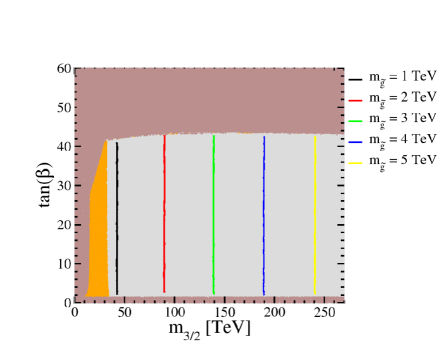
Figure 4.3: $\textrm{tan}\ \beta-m_{3/2}$ parameter space, with $\mu>0$ and $M_{\rm{string}}=M_{GUT}$. Also shown are gluino mass contours in the parameter plane.

Until now we have made the assumption that $M_{\rm{string}}=M_{GUT}$, but this is not necessarily so as pointed out earlier. In fact, we should expect that $M_{\rm{string}}$ will be somewhat lower than the GUT scale in order to have enough FCNC suppression. Figure 4.4 is a plot of the spectrum as a function of the string scale, and the latter is taken as low as $10^{11}$ GeV. As $M_{\rm{string}}$ is lowered the spectrum is seen to spread out, and there are cases of mass re-ordering. The most important feature of this plot is that around $5\times 10^{13}$ GeV, the LSP is the tau-sneutrino. There are severe limits on stable sneutrino dark matter [5]. Then, in order to avoid these limits and to have a ${\tilde{Z}}_{1}$ LSP, we do not consider such low $M_{\rm{string}}$.

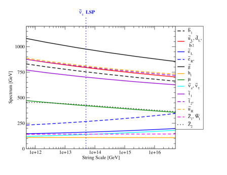
Figure 4.4: inoAMSBspectrum versus string scale for $m_{3/2}$ = 50 TeV, $\textrm{tan}\ \beta=10$, and $\mu>0$.

Finally, we also have been assuming that $m_{0}=0$. However this is not completely realistic, as they are only expected to be suppressed. The spectrum is shown again in Figure 4.5, this time as a function of $m_{0}$, the classical mass added universally to all scalars. We adopt values $m_{3/2}=50$ TeV and $\textrm{tan}\ \beta=10$ for this plot. As $m_{0}$ increases beyond zero, it is seen that the spectra change little so long as $m_{0}\stackrel{{\scriptstyle<}}{{\sim}}100$ GeV, and also the mass orderings remain intact. For larger values of $m_{0}$, the left- and right-slepton masses begin to increase, with first $m_{{\tilde{e}}_{R}}$ surpassing $m_{{\tilde{Z}}_{2}}$, and later even $m_{{\tilde{e}}_{L}}$ surpasses $m_{{\tilde{Z}}_{2}}$. At these high values of $m_{0}$, decay modes such as ${\tilde{Z}}_{2}\rightarrow\l^{\pm}{\tilde{l}}^{\mp}$ would become kinematically closed, thus greatly altering the collider signatures. However, generically in this class of models, we would not expect such large additional contributions to scalar masses.

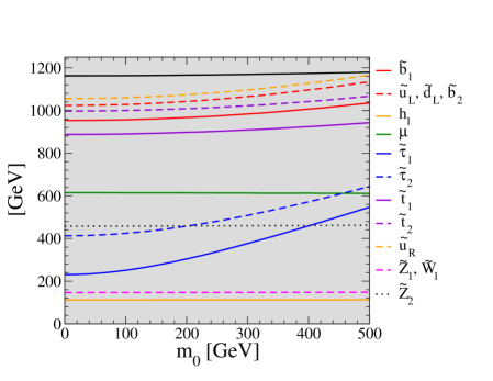
Figure 4.5: inoAMSBspectrum versus classical common soft mass, $m_{0}$. The parameters for this plot are $m_{3/2}=50$ TeV, $\textrm{tan}\ \beta=10$, and $\mu>0$.

BF($b\rightarrow s\gamma$) and (g-2)_μ/2

Along with experimental constraints on the inoAMSB models from LEP2 limits on $m_{h}$ and $m_{{\tilde{W}}_{1}}$, there also exist indirect limits on model parameter space from comparing measured values of $BF(b\to s\gamma)$ and $\Delta a_{\mu}\equiv(g-2)_{\mu}/2$ against SUSY model predictions. Figure 4.6 (a) shows regions of the branching fraction for $BF(b\rightarrow s\gamma)$ in the inoAMSB model versus $m_{3/2}$ and $\textrm{tan}\ \beta$ variation, calculated using the Isatools subroutine ISABSG[13]. The red-shaded region corresponds to branching fraction values within the SM theoretically predicted region $BF(b\rightarrow s\gamma)_{SM}=(3.15\pm 0.23)\times 10^{-4}$, by a recent evaluation by Misiak[84]). The blue-shaded region corresponds to branching fraction values within the experimentally allowed region [29]: here, the branching fraction $BF(b\to s\gamma)$ has been measured by the CLEO, Belle and BABAR collaborations; a combined analysis [29] finds the branching fraction to be $BF(b\to s\gamma)=(3.55\pm 0.26)\times 10^{-4}$. The gray shaded region gives too large a value of $BF(b\rightarrow s\gamma)$. This region occurs for low $m_{3/2}$, where rather light ${\tilde{t}}_{1}$ and ${\tilde{W}}_{1}$ lead to large branching fractions, or large $\textrm{tan}\ \beta$, where also the SUSY loop contributions are enhanced [14].
Figure 4.6 (b) shows the plot of the SUSY contribution to $\Delta a_{\mu}$: $\Delta a_{\mu}^{SUSY}$ (using ISAAMU from Isatools [17]). The contribution is large when $m_{3/2}$ is small; in this case, rather light ${\tilde{\mu}}_{L}$ and ${\tilde{\nu}}_{\mu L}$ masses lead to large deviations from the SM prediction. The SUSY contributions to $\Delta a_{\mu}^{SUSY}$ also increase with $\textrm{tan}\ \beta$. It is well-known that there is a discrepancy between the SM predictions for $\Delta a_{\mu}$, where $\tau$ decay data, used to estimate the hadronic vacuum polarization contribution to $\Delta a_{\mu}$, gives rough accord with the SM, while use of $e^{+}e^{-}\rightarrow hadrons$ data at very low energy leads to a roughly $3\sigma$ discrepancy. The measured $\Delta a_{\mu}$ anomaly, given as $(4.3\pm 1.6)\times 10^{-9}$ by the Muon $g-2$ Collaboration[39], is shown by the black dotted region.

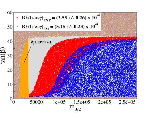
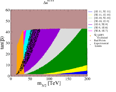
Figure 4.6: (a) $BF(b\rightarrow s\gamma)$ and (b) SUSY contribution to $(g-2)_{\mu}$ in the inoAMSBparameter plane with $M_{\rm{string}}=M_{GUT}$.

4.4 inoAMSBat the LHC

Sparticle Production

	mAMSB	HCAMSB1	inoAMSB1	inoAMSB2
$\sigma\ [{\rm fb}]$	$7.7\times 10^{3}$	$7.4\times 10^{3}$	$7.5\times 10^{3}$	$439$
${\tilde{g}},{\tilde{q}}\ {\rm pairs}$	15.0%	15.5%	19.1%	3%
${\rm EW-ino\ pairs}$	79.7%	81.9%	75.6%	93%
${\rm slep.}\ {\rm pairs}$	3.7%	0.8%	3.1%	3%
${\tilde{t}}_{1}\bar{\tilde{t}}_{1}$	0.4%	0.2%	0.1%	0%

Table 4.2: Cross sections for $pp\rightarrow SUSY$ at 14 TeV.

Table 4.2 shows the distributions in the cross section of various sparticle pair-production channels. EW-ino pairs dominate over all other forms of production. As in the case of HCAMSB, because ${\tilde{Z}}_{1}$ is stable and ${\tilde{W}}_{1}^{\pm}$ decays to soft $\pi^{\pm}$ and ${\tilde{Z}}_{1}$, the processes $pp\rightarrow{\tilde{W}}_{1}^{\pm}{\tilde{W}}_{1}^{\mp}$, ${\tilde{W}}_{1}^{\pm}{\tilde{Z}}_{1}$ do not produce sufficient visible energy to meet detector trigger requirements. We must instead rely on detecting produced squark and gluino pairs.
We will will be mainly interested in $pp\rightarrow{\tilde{g}}{\tilde{g}},{\tilde{q}}{\tilde{g}},{\tilde{q}}{\tilde{q}}$ because of their significant cross sections and visible final states. Figure 4.2 shows that there are significant cross sections for slepton production as well, but those cross sections are still lower than QCD pairs and the LHC reach in $m_{3/2}$ is much less. Therefore, for this analysis we focus strictly on QCD pair-production.
Since sparticle masses depend mainly on $m_{3/2}$, the plot of multiple pair-production cross sections is shown as a function of this parameter in Figure 4.7. We see that for $m_{3/2}\stackrel{{\scriptstyle<}}{{\sim}}$ 65 TeV ${\tilde{g}}{\tilde{q}}$ and ${\tilde{q}}{\tilde{q}}$ rates are comparable, but for higher $m_{3/2}$ that level squark pairs dominate. Rates for ${\tilde{g}}{\tilde{g}}$ can be significant, but they are never dominant.

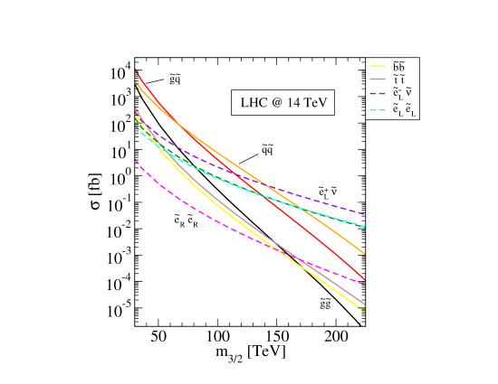
Figure 4.7: Production cross sections for various pairs versus $m_{3/2}$ for $\textrm{tan}\ \beta$ = 10, and $\mu>0.$

Sparticle Decay

We saw that the inoAMSBRGE running leads to a hierarchy of masses in which all squark masses are close in value and less than the gluino mass. Thus, produced gluinos decay nearly equally to squark species through ${\tilde{g}}\rightarrow q{\tilde{q}}$. Left squarks decay mainly through ${\tilde{q}}_{L}\rightarrow q+wino$, and the calculation shows ${\tilde{q}}_{L}\rightarrow q^{\prime}{\tilde{W}}_{1}$ at 67% and ${\tilde{q}}_{L}\rightarrow q{\tilde{Z}}_{1}$ at 33% over the entire parameter space. Right squarks on the other hand decay to $q+bino$, and therefore the decays ${\tilde{q}}_{R}\rightarrow q{\tilde{Z}}_{2}$ occur at 97% over all the parameter values.
The RGE evolution also led to a large left-right splitting in the sleptons, and this should have noticeable effects. Left sleptons decay mainly to $wino+lepton$ and the calculation shows ${\tilde{l}}_{L}\rightarrow l{\tilde{Z}}_{1}$ at 33% and ${\tilde{l}}_{L}\rightarrow\nu_{lL}{\tilde{W}}_{1}$ at 67% over all parameters. Sneutrinos decay invisibly to $\nu_{l}{\tilde{Z}}_{1}$ at 33%, but has 66% visible branching to $l{\tilde{W}}_{1}$. If right-sleptons were heavy enough, they would decay to $bino+lepton$, but since they are too light they decay via ${\tilde{l}}_{R}\rightarrow$ $e{\tilde{Z}}_{1}$ at 78%, as well as through three-body modes ${\tilde{l}}^{-}_{R}\rightarrow$ $l^{-}\tau^{+}{\tilde{\tau}}_{1}^{-}$ and $l^{-}\tau^{-}{\tilde{\tau}}_{1}^{+}$ at 13% and 7% respectively.

inoAMSBLHC Events

Isajet [88] was used for the LHC event simulation, the details of which can be found in Section 1.5. Two-million events for inoAMSBpoint 1 of Table 4.1 were generated in addition to the same Standard Model backgrounds discussed in the Chapter 3, which are $W+jets,\ \ Z+jets$, $t\bar{t},\ \ WW,\ \ WZ$, and $ZZ$.
We first apply a rudimentary set of cuts on signal and background that we will label C1. This first round of cuts will help to understand the underlying properties of LHC events and will give us information on how to make better cuts. The C1 cuts are as follows:

• $n(jets)\geq 2$

• $\not{E}_{T}>max(100\ \textrm{GeV},0.2M_{eff})$

• ${E_{T}}(j_{1},j_{2})>100,50\ \textrm{GeV}$

• transverse sphericity $S_{T}>0.2$,

where $M_{eff}=\not{E}_{T}+{E_{T}}(j_{1})+{E_{T}}(j_{2})+{E_{T}}(j_{3})+{E_{T}}(j_{4})$.
Since the sparticle production is dominated by ${\tilde{g}}{\tilde{q}}$ and ${\tilde{q}}{\tilde{q}}$ we expect to have two very hard jets in each event through the squark decays to EW-ino + quark. This is seen in Figure 4.8 where the first and second hardest ${p_{T}}$ distributions are seen to emerge from background around 450 GeV and 250-300 GeV respectively.

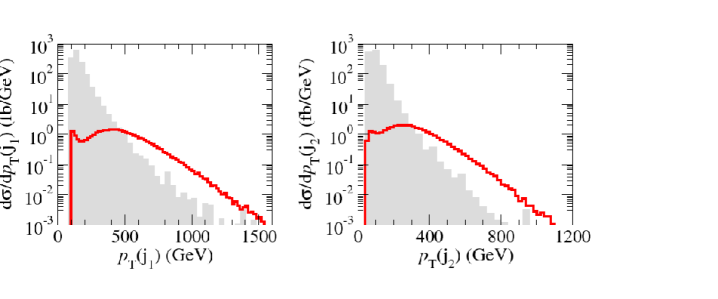
Figure 4.8: ${p_{T}}$ distributions for hardest (left) and second hardest (right) jets for inoAMSB1 and SM backgrounds after C1 cuts for 14 TeV pp collisions.

Figure 4.9 shows the $\not{E}_{T}$ and $A_{T}(=\not{E}_{T}+\sum^{jets}{E_{T}}+\sum^{isolated\atop leptons}{E_{T}}$) distributions for inoAMSB1 with SM backgrounds. The $\not{E}_{T}$ distribution emerges from background around 500 GeV and appears rather hard because squarks have a significant invisible branching to ${\tilde{Z}}_{1}$s. The $A_{T}$ distribution has a peak around 400 GeV that is buried under background, and a broad hard peak at higher $A_{T}$. The softer peak originates in chargino, neutralino, and slepton pair production, while the hard peak is due to squark and gluino pair production and emerges from background around 1400 GeV.

Figure 4.9: ${E_{T}}$ and $A_{T}$ distributions for inoAMSB1 and SM backgrounds after C1 cuts for 14 TeV pp collisions.

We also examine jet (left) and lepton (right) multiplicities in Figure 4.10. We expect to see hard dijet events from squark decays, but the jet distribution shows a broad peak between $n_{j}=$ 2–5 as well as much higher values. These extra jets occur because of cascade decays and ISR and because in this first round of cuts $\not{E}_{T}>$ 50 GeV which is rather low compared to when the hardest jets exceed background in Figure 4.8. The leptons are seen to stand out above background already at 3 leptons, and so we see already that with the minimal cuts a signal with 3 leptons, at least 2 jets, and $\not{E}_{T}$ should appear well above background.

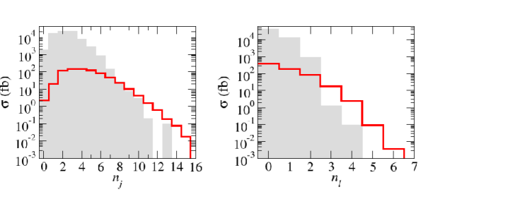
Figure 4.10: Jet multiplicity (left) and lepton multiplicity (right) distributions for inoAMSB1 and SM backgrounds after C1 cuts for 14 TeV pp collisions.

Again, as was the case for mAMSBand HCAMSBalready encountered, HITs (see Section 2) from long-lived charginos is an important signal for models with wino-like ${\tilde{Z}}_{1}$s, particularly AMSB models. If the anomaly mediation supersymmetry breaking pattern is the correct one, we expect HITs to play an important role in the discovery of SUSY at the LHC. After an AMSB discovery, deciphering further whether a model is correct would be the next step. After discussing the reach in the next subsection, it will be shown that if mAMSB, HCAMSB, and inoAMSBare accessible at the LHC, it would be possible to unambiguously distinguish between all three models! This is a major result of this work.

LHC Reach

Now we would like to find what are the maximum inoAMSBparameter values accessible at the LHC after one year of data collection (100 ${\textrm{fb}^{-1}}$) at $\sqrt{s}=$ 14 TeV. This amounts to finding the reach in the $m_{3/2}$ parameter because it makes the most significant contribution to sparticle mass as seen in Figure 4.2.
Taking what was learned in the last section by the C1 cuts on signal and background, we adopt the following new set of cuts labeled C2:

• $n(jets)\geq 2$

• $S_{T}>0.2$

• ${E_{T}}(j_{1}),\ {E_{T}}(j_{2}),\ \not{E}_{T}\ >\ {E_{T}^{c}}$

where ${E_{T}^{c}}$ is variable in order to maximize the reach. Parameter space points with lower masses benefit from lower ${E_{T}^{c}}$. Heavier particles have lower cross sections but also have higher energy release per event and thus are more visible for higher ${E_{T}^{c}}$. Additionally, we apply extra cuts for multilepton channels. For the $0l$ channel we apply a cut on the transverse opening angle between $\not{E}_{T}$ and the nearest jet, $30^{\circ}<$ $\Delta\phi(\not{E}_{T},{E_{T}}(j^{near})<90^{\circ})$. For all isolated leptons a minimum ${p_{T}}$ of 20 GeV is required. For the sake of brevity we will consider $0l,2l(OS),3l,\textrm{and}\ 4l$ channels because they provide the best reach.
After applying C2 cuts with ${E_{T}^{c}}=100$ GeV on SM backgrounds (2M events each) and the inoAMSB1 point, the total cross sections are shown in Table 4.3. The hard C2 cuts prevent some backgrounds from producing noticeable cross sections indicated in the table by dashes. For a signal to be considered observable, we require that i.) $S/B>0.2$, ii.) Signal has at least 5 events, and iii.) $S>5\sqrt{B}$ (5$\sigma$ significance), where $S$ and $B$ are respectively the signal and the background numbers of events for a given luminosity.

Process	$0\ell$	$OS$	$SS$	$3\ell$	$4\ell$
QCD($p_{T}$: 0.05-0.10 TeV)	–	–	–	–	–
QCD($p_{T}$: 0.10-0.20 TeV)	755.1	–	–	–	–
QCD($p_{T}$: 0.20-0.40 TeV)	803.8	621.1	109.6	36.5	–
QCD($p_{T}$: 0.40-1.00 TeV)	209.8	304.7	72.6	29.0	2.6
QCD($p_{T}$: 1.00-2.40 TeV)	2.2	5.3	1.7	1.5	0.2
$t\bar{t}$	1721.4	732.6	273.8	$113.3$	$6.6$
$W+jets;W\to e,\mu,\tau$	527.4	22.6	8.4	$1.3$	$--$
$Z+jets;Z\to\tau\bar{\tau},\ \nu s$	752.9	11.1	1.3	$0.2$	$--$
$WW,ZZ,WZ$	3.4	0.3	$0.25$	$--$	$--$
$Summed\ SM\ BG$	4776.1	1697.8	467.7	$181.9$	$9.4$
inoAMSB1	112.7	85.7	27.6	36.0	7.5

Table 4.3: Estimated SM background cross sections and the inoAMSB1 benchmark point in fb for various multi-lepton plus jets $+\not{E}_{T}$ topologies after cuts C2 with ${E_{T}^{c}}=100$ GeV.

Applying these criteria, the model’s $m_{3/2}$ reach after 100 ${\textrm{fb}^{-1}}$ of data collection is computed for each of the lepton channels and for each of ${E_{T}^{c}}=100,300$ and 500 GeV. Figure 4.11 shows the plots of the cross section for the background (horizontal) and signal (decreasing slopes) as a function of $m_{3/2}$. In the figure solid blue represents cuts with ${E_{T}^{c}}=100$ GeV, red dash-dotted represents 300 GeV, and purple dashed represents 500 GeV. Where the signal touches its corresponding (5$\sigma$) background value on the plot is the where signal is no longer significant enough to be observable. These $m_{3/2}$ values are listed in Table 4.4 (along with the SS dilepton reach). It is seen there that the best reach at 100 ${\textrm{fb}^{-1}}$ for the inoAMSB model (with $\textrm{tan}\ \beta=10$ and $\mu>0$) is for multi-jet + $\not{E}_{T}$ + 3l which shows significant cross section up to $m_{3/2}\sim 118$ TeV ($m_{\tilde{g}}\sim 2.6$ TeV) when ${E_{T}^{c}}=$ 500 GeV.

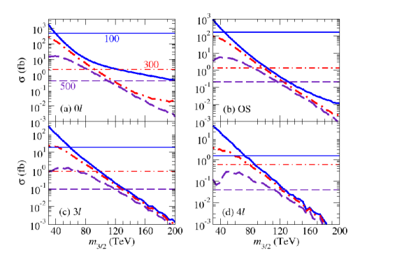
Figure 4.11: Cross section for multi-jet plus $\not{E}_{T}$ events with a). $n(\ell)=0$, b). OS isolated dileptons c). isolated $3\ell$s and d). isolated $4\ell$s at the LHC after cuts $C2$ listed in the text with $E_{T}^{c}=100$ GeV (blue solid), $E_{T}^{c}=300$ GeV (red dot-dashed) and $E_{T}^{c}=500$ GeV (purple dashes), versus $m_{3/2}$, from the inoAMSB model line points with $\tan\beta=10$ and $\mu>0$. We also list the 100 fb^-1 $5\sigma$, 5 event, $S>0.1\ BG$ limit with the horizontal lines.

$E_{T}^{c}$ (GeV)	$0\ell$	$OS$	$SS$	$3\ell$	$4\ell$
100	$40$	$57$	62	$60$	$75$
300	$93$	$95$	85	$98$	$80$
500	$110$	$115$	105	$118$	$110$

Table 4.4: Estimated reach of 100 fb^-1 LHC for $m_{3/2}$ (TeV) in the inoAMSB model line in various signal channels.

HITs + multi-peak $m(l^{+}l^{-})$ Distribution

We next examine the dilepton invariant mass distribution for cascade decay events for $\geq 2$ high ${p_{T}}$ jets, large $\not{E}_{T}$ and $SF/OS$ dileptons. It is known that the $m(l^{+}l^{-})$ distribution is capable of having a “kinematic mass edge” structure through the decay ${\tilde{Z}}_{2}\rightarrow{\tilde{l}}^{\pm}l^{\mp}$ or through ${\tilde{Z}}_{2}\rightarrow l^{\pm}l^{\mp}{\tilde{Z}}_{1}$[87]. Because the inoAMSBmodel predicts L/R splitting in the slepton masses, so it is expected that two edges can occur from the first type of decay through ${\tilde{Z}}_{2}\rightarrow{\tilde{l}}_{L}^{\pm}l^{\mp}$ and ${\tilde{Z}}_{2}\rightarrow{\tilde{l}}_{R}^{\pm}l^{\mp}$.
It is also expected that a peak can occur in the $m(l^{+}l^{-})$ distribution around $M_{Z}$ because of the decays ${\tilde{Z}}_{3}\rightarrow Z{\tilde{Z}}_{1}$, ${\tilde{Z}}_{4}\rightarrow Z{\tilde{Z}}_{1}$ and ${\tilde{W}}_{2}\rightarrow Z{\tilde{W}}_{1}$. In the case of point inoAMSB1, these branching occur for 25%, 6%, and 29% respectively.
Figure 4.12 frame (a) shows the $m(l^{+}l^{-})$ distribution for inoAMSB1 (red line) along with mAMSB(green) and HCAMSB(blue) points. The cuts are C1 with $\not{E}_{T}>300$ GeV and $A_{T}>$ 900 GeV, and the SM backgrounds are completely suppressed. The peak at $M_{Z}$ is clear and there is a ${\tilde{Z}}_{2}$ decay double-edge structure calculated to be at values

$$m(l^{+}l^{-})\leq m_{{\tilde{Z}}_{2}}\sqrt{1-\frac{m_{{\tilde{l}}}^{2}}{m_{{\tilde{Z}}_{2}}^{2}}}\sqrt{1-\frac{m_{{\tilde{Z}}_{1}}^{2}}{m_{{\tilde{l}}}^{2}}}=\textrm{182 GeV and 304 GeV.}$$ (4.19)

The former is for ${\tilde{Z}}_{2}$ to ${\tilde{l}}_{R}$ decays where as the latter is for the decays to left-sleptons.

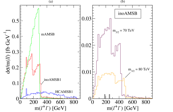
Figure 4.12: Dilepton invariant mass distribution. (a) comparison of inoAMSBto mAMSBand HCAMSB. C1 cuts are used with $\not{E}_{T}>300$ GeV and $A_{T}>900GeV$. (b) the same distribution except $m_{3/2}=70$ and 80 TeV values. The double-edge is still visible at these high $m_{3/2}$ values.

Unlike inoAMSB, the mAMSBplot exhibits only a single edge because mAMSBpoints predict nearly-degenerate L and R sleptons. mAMSBalso lacks a Z-peak because the second heaviest neutralino, ${\tilde{Z}}_{2}$, is bino-like and thus has suppressed couplings to ${\tilde{Z}}_{1}Z$. HCAMSBdoes not have an edge because here ${\tilde{Z}}_{2}$ is higgsino-like and has different decay products: ${\tilde{Z}}_{2}\rightarrow{\tilde{W}}_{1}^{\pm}W^{\mp}$, ${\tilde{Z}}_{1}h$, and ${\tilde{Z}}_{1}Z$. Because the last decay channel should always be open, HCAMSBhas a smooth $m(l^{+}l^{-})$ distribution with a visible Z-resonance.
We conclude that inoAMSB, mAMSB, and HCAMSBmodels can be distinguished at the LHC. First, AMSB models in general are identified by a wino-like ${\tilde{Z}}_{1}$ with near degeneracy to the lightest chargino. This would be seen in gluino and squark cascade decay events including a long-lived chargino with a terminating track (HIT signal). Then the different $m(l^{+}l^{-})$ distributions could be used to distinguish between the inoAMSB, HCAMSB, or mAMSBcases. These results are summarized in Table 4.5 for the reader’s convenience.

Model	HITs	# of edges	${\tilde{Z}}_{2}$	$m_{{\tilde{l}}_{L}}\stackrel{{\scriptstyle?}}{{\approx}}m_{{\tilde{l}}_{R}}$
inoAMSB	Yes	2	bino	No
mAMSB	Yes	1	bino	Yes
HCAMSB	Yes	0	higgsino	No

Table 4.5: The three AMSB models can be distinguished in the dilepton invariant mass distribution by the number of edges. The structures depend crucially on the type of ${\tilde{Z}}_{2}$ and the slepton masses predicted by the models.

4.5 Summary

In this chapter, we have examined the phenomenology of supersymmetric models with the boundary conditions $m_{0}\sim A_{0}\sim 0$ at $M_{string}$, while gaugino masses assume the form as given in AMSB. We have labeled this class of boundary conditions gaugino-AMSB boundary conditions, or inoAMSBfor short. Such boundary conditions can arise in type IIB string models with flux compactifications. They are very compelling in that off-diagonal flavor violating and also $CP$ violating terms are highly suppressed, as in the case of no-scale supergravity or gaugino-mediated SUSY breaking models. However, since gaugino masses assume the AMSB form at $M_{GUT}$, the large $U(1)_{Y}$ gaugino mass $M_{1}$ pulls slepton masses to large enough values through renormalization group evolution that one avoids charged LSPs (as in NS or inoMSB model) or tachyonic sleptons (as in pure AMSB models).
The expected sparticle mass spectrum is very distinctive. Like mAMSB and HCAMSB, it is expected that lightest neutralino (${\tilde{Z}}_{1}$) will be wino-like, and a quasi-stable chargino (${\tilde{W}}_{1}$) would leave observable highly ionizing tracks in collider detectors. The spectrum is unlike mAMSB in that a large mass splitting is expected between left- and right- sleptons. The case when the string scale, $M_{string}$, is much lower than $M_{GUT}$ was also investigated. In this case, the entire spectrum becomes somewhat spread-out, and if $M_{s}\stackrel{{\scriptstyle<}}{{\sim}}10^{14}$ GeV, then the left-sneutrino becomes the LSP, which is excluded by double beta decay experiments [5].
We also saw in detail some aspects of LHC collider signatures. Since $m_{{\tilde{q}}}<m_{{\tilde{g}}}$ in inoAMSB models, we expect dominant ${\tilde{q}}{\tilde{q}}$ and ${\tilde{q}}{\tilde{g}}$ production at LHC, followed by 2-body ${\tilde{q}}$ and ${\tilde{g}}$ decays. This leads to collider events containing at least two very high $p_{T}$ jets plus $\not{E}_{T}$ as is indicative of squark pair production.
While squark and gluino cascade decay events should be easily seen at the LHC (provided $m_{3/2}\stackrel{{\scriptstyle<}}{{\sim}}110$ TeV), the signal events should all contain visible HITs, which would point to a model with $m_{{\tilde{W}}_{1}}\simeq m_{{\tilde{Z}}_{1}}$, as occurs in anomaly-mediation where $M_{2}<M_{1},\ M_{3}$ at the weak scale. We find a LHC reach, given 100 fb^-1 of integrated luminosity, out to $m_{3/2}\sim 118$ TeV, corresponding to a reach in $m_{{\tilde{g}}}$ of about 2.6 TeV. We note here that if a signal is found at the outer edges of the reach limit, the signal will consist of typically just a few (5-10) events (due to hard cuts) over a small background. The signal events should include the characteristic presence of HITs, which should be absent in the background. As data accumulates, signals should also appear in the complementary channels, thus building confidence in a discovery.
We also find that the invariant mass distribution of SF/OS dilepton pairs should have a distinctive two-bump structure that is indicative of neutralino decays through both left- and right- sleptons with a large slepton mass splitting. This distribution would help distinguish inoAMSB models from HCAMSB, where a continuum plus a $Z$-peak distribution is expected, or from mAMSB, where the two mass edges (present only if $m_{0}$ is small enough that $m_{{\tilde{l}}_{L}}$ and $m_{{\tilde{l}}_{R}}$ are lighter than $m_{{\tilde{Z}}_{2}}$) would be very close together, and probably not resolvable.

5 Dark Matter in AMSB Models

5.1 Introduction to Dark Matter in AMSB Models

Now that we know what to expect for mAMSB, HCAMSB, and inoAMSBmodels at the LHC, we can now turn our attention to using astrophysical methods to observe them. In particular we are interested in i) whether these models can account for the observed cold dark matter (CDM) abundance

$$\Omega h^{2}=0.1123\pm 0.0035\ \ 68\%CL$$ (5.1)

according to WMAP7 [75] measurements, where $\Omega=\frac{\rho}{\rho_{c}}$, and $\rho_{c}=1.88\times 10^{-29}\ h^{2}$ ${\rm g\ cm^{-3}}$ is the critical closure density; ii) if current or future experiments can either confirm or rule out regions of their parameter spaces; and iii) how cosmological data compares with LHC data.
At first sight there appear to be problems with AMSB models arising from the fact that the LSPs annihilate and co-annihilate (with the lightest chargino) too efficiently [41] and leave the relic density of thermally produced neutralinos 1–2 orders of magnitude below the experimental value in Equation 5.1. Indeed, this is a major issue with AMSB models that has led many to consider other model types to be more interesting. However, it is argued here that when one looks back into the history of the Universe it is important not only to consider thermal production of LSPs in quasi-thermal equilibrium, but it is also important to consider the impact of non-thermal production of LSPs: production of LSPs through the decay of heavy particles that may have existed early on.
In this chapter we will explore several possibilities to increase the CDM abundance(s) that are strongly motivated in theory. String theories require the presence of heavy moduli fields (and other heavy scalars) and local SUSY theories require gravitinos, both of which decay through gravitational interactions and can add to $\Omega h^{2}$. We also consider here the case where the strong CP problem is solved by invoking the axion ($a$) solution. When this solution is combined with the SUSY framework, the axion’s supersymmetric partner, the axino ($\tilde{a}$), appears in the spectrum [93] and its mass is tied (model-dependently) to the SUSY breaking sector. This means that the axino can be heavy enough that its decay chains terminate with LSP production or it can even serve as the LSP itself and contribute, along with the axion, to the CDM abundance.
Non-thermal production mechanisms must not only produce enough DM to account for WMAP, but must also be careful not to disrupt Big Bang Nucleosynthesis (BBN) which includes measurements of light element abundances, baryon-entropy ratio, and the neutron-proton ratio. With these requirements being met, the AMSB models’ parameters can be further constrained and the reaches will be shown for direct and indirect detection experiments.
This chapter is organized as follows. In Section 5.2, four non-thermal production mechanisms of dark matter will be described. The first two result in an increase of wino-neutralino DM as a result of moduli decay and (thermally-produced) gravitino decay. The remaining mechanisms will invoke the Peccei-Quinn (PQ) solution to the strong CP problem. The third mechanism will increase the wino DM through heavy axino decays and there will be an additional component of axion (a) DM from the breaking of the PQ symmetry. In the fourth mechanism we take the axino ($\tilde{a}$) to be the LSP such that it is produced both thermally and in neutralino decays. This last case will have a mixture of axion and axino CDM.
Dark matter may be observable in future experiments through direct detection (DD) where the relic DM particles scatter from target nuclei in the experimental apparatus. It is also possible that it will be observed through indirect detection (ID) where DM annihilate into SM particles somewhere else in the galaxy and we see its products. A brief description of CDM experiments is given Section 5.3.
Sections 5.4 and 5.5 contain the results of this research. In Section 5.4, the calculated DD cross sections for AMSB wino DM are given. In Section 5.5, the ID rates for mAMSB, HCAMSB, and inoAMSBmodels are also given. The discussions in these sections describe the interactions that lead to the calculated rates and explore the current experimental exclusions and future experimental reaches of the parameter space. Finally, we close this chapter in Section 5.6 with a summary and conclusion.

5.2 Thermal and Non-thermal Production of Dark Matter in AMSB Models

As described in the Introduction of this chapter, dark matter (DM) production in the early universe can happen both thermally and non-thermally. In this section we explore four cases where the abundance of DM is composed of thermal and non-thermal components. In addition, we will see in these cases the DM can be wino (as for our AMSB models), axion, axino, or mixtures of these.

Neutralino CDM via Moduli Decay

Shortly after the introduction of AMSB models, Moroi and Randall proposed a solution to the AMSB dark matter problem based on augmented neutralino production via the decays of moduli fields in the early universe [85]. The idea here is that string theory is replete with additional moduli fields: neutral scalar fields with gravitational couplings to matter. In generic supergravity theories, the moduli fields are expected to have masses comparable to $m_{3/2}$. When the Hubble expansion rate becomes comparable to the moduli mass $m_{\phi}$, then an effective potential will turn on, and the moduli field(s) will oscillate about their minima, producing massive excitations, which will then decay to all allowed modes: e.g. gauge boson pairs, higgs boson pairs, gravitino pairs, $\cdots$. The neutralino production rate via moduli decay has been estimated in Ref. [85]. It is noted in Ref. [2] that the abundance– given by

$$\Omega_{{\tilde{Z}}_{1}}^{mod.}h^{2}\sim 0.1\times\left(\frac{m_{{\tilde{Z}}_{1}}}{100\ {\rm GeV}}\right)\left(\frac{10.75}{g_{*}}\right)^{1/4}\left(\frac{\sigma_{0}}{\langle\sigma v\rangle}\right)\left(\frac{100\ {\rm TeV}}{m_{\phi}}\right)^{3/2}$$ (5.2)

with $\sigma_{0}=3\times 10^{-24}$ cm³/sec – yields nearly the measured dark matter abundance for wino-like neutralino annihilation cross sections and $m_{\phi}\sim 100$ TeV. These authors dub this the “non-thermal WIMP miracle”.
A necessary condition for augmented neutralino production via scalar field decay is that the re-heat temperature of radiation $T_{R}$ induced by moduli decays is bounded by $T_{R}\stackrel{{\scriptstyle>}}{{\sim}}5$ MeV (in order to sustain Big Bang Nucleosynthesis (BBN) as we know it), and $T_{R}<T_{fo}$, where $T_{fo}$ is the freeze-out temperature for thermal neutralino production $T_{fo}\sim m_{{\tilde{Z}}_{1}}/20$. If $T_{R}$ exceeds $T_{fo}$, then the decay-produced neutralinos will thermalize, and the abundance will be given by the thermal calculation as usual.
This “low re-heat” neutralino production mechanism has been investigated extensively by Gondolo, Gelmini, et. al. [58][57][56]. The low re-heat neutralino abundance calculation depends on the input value of $T_{R}$ and the ratio $b/m_{\phi}$, where $b$ is the average number of neutralinos produced in moduli decay, and $m_{\phi}$ is the scalar field mass. They note that theories with an under-abundance of thermally produced neutralino CDM with $\Omega_{{\tilde{Z}}_{1}}^{TP}\stackrel{{\scriptstyle>}}{{\sim}}10^{-5}\left(\frac{100\ {\rm GeV}}{m_{{\tilde{Z}}_{1}}}\right)$ can always be brought into accord with the measured DM abundance for at least one and sometimes two values of $T_{R}$.
While the low $T_{R}\sim 10-1000$ MeV scenario with DM generation via scalar field decay is compelling, we note here that it is also consistent with some baryogenesis mechanisms: e.g. Affleck-Dine baryogenesis wherein a large baryon asymmetry is generated early on, only to be diluted to observable levels via moduli decay [69], or a scenario wherein the baryon asymmetry is actually generated by the moduli decay [71].

Neutralino CDM via Gravitino Decay

An alternative possibility for augmenting the production of wino-like neutralinos in AMSB models is via gravitino production and decay in the early universe. While gravitinos would not be in thermal equilibrium during or after re-heat, they still can be produced thermally via radiation off ordinary sparticle scattering reactions in the early universe. The relic density of thermally produced gravitinos as calculated in Ref’s [92] [36] is given by

$$\Omega_{\tilde{G}}^{TP}h^{2}=\sum_{i=1}^{3}\omega_{i}g_{i}^{2}\left(1+\frac{M_{i}^{2}}{3m_{3/2}^{2}}\right)\log\left(\frac{k_{i}}{g_{i}}\right)\left(\frac{m_{3/2}}{100\ {\rm GeV}}\right)\left(\frac{T_{R}}{10^{10}\ {\rm GeV}}\right),$$ (5.3)

where $g_{i}$ and $M_{i}$ are the gauge couplings and gaugino masses evaluated at scale $Q=T_{R}$, and $\omega_{i}=(0.018,0.044,0.117)$ and $k_{i}=(1.266,1.312,1.271)$. Each gravitino ultimately cascade decays down to the wino-like ${\tilde{Z}}_{1}$ state, so the neutralino relic density is given by

$$\Omega_{{\tilde{Z}}_{1}}h^{2}=\Omega_{{\tilde{Z}}_{1}}^{TP}h^{2}+\frac{m_{{\tilde{Z}}_{1}}}{m_{3/2}}\Omega_{\tilde{G}}^{TP}h^{2}.$$ (5.4)

A plot of the value of $T_{R}$ and $m_{3/2}$ which is required to yield $\Omega_{{\tilde{Z}}_{1}}h^{2}=0.11$ from Equation 5.4 is shown in Figure 5.1 for mAMSB ($m_{0}=0.01m_{3/2}$), HCAMSB ($\alpha=0.02$) and inoAMSB using $\tan\beta=10$ and $\mu>0$. The region above the $\Omega_{{\tilde{Z}}_{1}}h^{2}=0.11$ curves would yield too much dark matter, while the region below the curves yields too little.

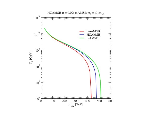
Figure 5.1: Plot of allowed region of $T_{R}\ vs.\ m_{3/2}$ plane allowed for wino-like neutralino DM from thermal production plus thermally produced gravitino decay. For HCAMSB $\alpha=0.02$ and for mAMSB $m_{0}=0.01\ m_{3/2}$.

We should consider the curves shown in Figure 5.1 as only indicative of the simplest scenario for wino production via gravitino decay. Three other effects can substantially change the above picture from what is presented in Equation 5.4.

• On the one hand, if moduli fields $\phi_{m}$ exist with mass $m_{\phi_{m}}>2m_{3/2}$, then gravitinos can also be produced via moduli production and decay [73][10]. The exact abundance of these moduli-produced gravitinos is very model dependent, and depends on the moduli and gravitino mass and branching fractions.

• A second case arises if we consider gravitino production via inflaton decay at the end of inflation [51]. This production mechanism depends on unknown properties of the inflaton: e.g. its mass and branching fractions, and the re-heat temperature generated by inflaton decay. These latter quantities are very model dependent.

• Additional entropy production generated via the inflaton, moduli and gravitino decays may also dilute the above relic abundance in Equation 5.4.

We will bear in mind that these possibilities permit much lower or much higher values of $T_{R}$ and $m_{3/2}$ than those shown by the $\Omega_{{\tilde{Z}}_{1}}h^{2}=0.1$ contour of Figure 5.1.

Neutralino CDM from Heavy Axino Decays Mixed with Axion CDM

A third mechanism for increasing the wino-like relic abundance is presented in Ref. [43], in the context of the PQMSSM. If we adopt the Peccei- Quinn (PQ) solution to the strong $CP$ problem within the context of supersymmetric models, then it is appropriate to work with the PQ-augmented MSSM, which contains in addition to the usual MSSM states, the axion $a$, the $R$-parity even saxion field $s$, and the spin-${1\over 2}$ $R$-parity odd axino ${\tilde{a}}$. The axino can serve as the lightest SUSY particle if it is lighter than the lightest $R$-odd MSSM particle. The $a$ and ${\tilde{a}}$ have couplings to matter which are suppressed by the value of the PQ breaking scale $f_{a}$, usually considered to be in the range $10^{9}\ {\rm GeV}\stackrel{{\scriptstyle<}}{{\sim}}f_{a}\stackrel{{\scriptstyle<}}{{\sim}}10^{12}$ GeV[11].
In Ref. [43], it is assumed that $m_{{\tilde{a}}}>m_{{\tilde{Z}}_{1}}$, where ${\tilde{Z}}_{1}$ is the LSP. In the AMSB scenarios considered here, we will assume $T_{R}\stackrel{{\scriptstyle<}}{{\sim}}10^{10}$ GeV, so as to avoid overproduction of dark matter via gravitinos. With these low values of $T_{R}$, we are also below the axino decoupling temperature $T_{{\tilde{a}}-dcp}=10^{11}\ {\rm GeV}\left(\frac{f_{a}}{10^{12}\ {\rm GeV}}\right)^{2}\left(\frac{0.1}{\alpha_{s}}\right)^{3}$, so the axinos are never considered at thermal equilibrium [93]. However, axinos can still be produced thermally via radiation off usual MSSM scattering processes at high temperatures. The calculation of the thermally produced axino abundance, from the hard thermal loop approximation, yields [37]

$$\Omega_{{\tilde{a}}}^{TP}=h^{2}\simeq 5.5g_{s}^{6}\ln\left(\frac{1.211}{g_{s}}\right)\left(\frac{10^{11}\ {\rm GeV}}{f_{a}/N}\right)^{2}\left(\frac{m_{{\tilde{a}}}}{0.1\ {\rm GeV}}\right)\left(\frac{T_{R}}{10^{4}\ {\rm GeV}}\right)$$ (5.5)

where $g_{s}$ is the strong coupling evaluated at $Q=T_{R}$ and $N$ is the model dependent color anomaly of the PQ symmetry, of order 1. Since these axinos are assumed quite heavy, they will decay to $g{\tilde{g}}$ or ${\tilde{Z}}_{i}\gamma$ modes, which further decay until the stable LSP state, assumed here to be the neutral wino, is reached.
If the temperature of radiation due to axino decay ($T_{D}$) exceeds the neutralino freeze-out temperature $T_{fo}$, then the thermal wino abundance is unaffected by axino decay. If $T_{D}<T_{fo}$, then the axino decay will add to the neutralino abundance. However, this situation breaks up into two possibilities: i). a case wherein the axinos can dominate the energy density of the universe, wherein extra entropy production from heavy axino decay may dilute the thermal abundance of the wino-like LSPs, and ii). a case where they don’t. In addition, if the yield of winos from axino decay is high enough, then additional annihilation of winos after axino decay may occur; this case is handled by explicit solution of the Boltzmann equation for the wino number density. Along with a component of wino-like neutralino CDM, there will of course be some component of vacuum mis-alignment produced axion CDM: thus, in this scenario, we expect a WIMP/axion mixture of CDM.

Mixed Axion/Axino CDM

In this case, we again consider the PQMSSM, as in the last subsection. But now, we consider a light axino with $m_{{\tilde{a}}}<m_{{\tilde{Z}}_{1}}$, so that ${\tilde{a}}$ is the stable LSP [44]. Here, the thermally produced wino-like neutralinos will decay via ${\tilde{Z}}_{1}\to{\tilde{a}}\gamma$, so we will obtain a very slight dark matter abundance from neutralino decay: $\Omega_{{\tilde{a}}}^{NTP}=\frac{m_{{\tilde{a}}}}{m_{{\tilde{Z}}_{1}}}\Omega_{{\tilde{Z}}_{1}}h^{2}$, since each thermally produced neutralino gives rise to one non-thermally produced (NTP) axino. We will also produce axinos thermally via Equation 5.5. Finally, we will also produce axion CDM via the vacuum mis- alignment mechanism[1]: $\Omega_{a}h^{2}\simeq\frac{1}{4}\left(\frac{f_{a}/N}{10^{12}\ {\rm GeV}}\right)^{7/6}\theta_{i}^{2}$ (we will take here the initial mis-alignment angle $\theta_{i}\simeq 1$). The entire CDM abundance is then the sum

$$\Omega_{a{\tilde{a}}}h^{2}=\Omega_{{\tilde{a}}}^{NTP}h^{2}+\Omega_{{\tilde{a}}}^{TP}h^{2}+\Omega_{a}h^{2}.$$ (5.6)

In this case, the TP axinos constitute CDM as long as $m_{{\tilde{a}}}\stackrel{{\scriptstyle>}}{{\sim}}0.1$ MeV. The NTP axinos constitute warm DM for $m_{{\tilde{a}}}\stackrel{{\scriptstyle<}}{{\sim}}1$ GeV [63], but since their abundance is tiny, this fact is largely irrelevant. The entire CDM abundance then depends on the parameters $f_{a}$, $m_{{\tilde{a}}}$ and $T_{R}$; it also depends extremely weakly on $\Omega_{{\tilde{Z}}_{1}}h^{2}$, since this is usually small in AMSB models.
As an example, we plot in Fig. 5.2 the three components of mixed axion/axino DM abundance from HCAMSB benchmark point 1 in Reference [25]: $\alpha=0.025$, $m_{3/2}=50$ TeV, $\tan\beta=10$ and $\mu>0$. The neutralino thermal DM abundance would be $\Omega_{{\tilde{Z}}_{1}}h^{2}=0.0015$ if the ${\tilde{Z}}_{1}$ was stable. We require instead $\Omega_{a{\tilde{a}}}h^{2}=0.11$, and plot the three components of $\Omega_{a{\tilde{a}}}h^{2}$ versus $f_{a}/N$, for three values of $T_{R}=10^{6}$, $10^{7}$ and $10^{8}$ GeV. The value of $m_{{\tilde{a}}}$ is determined by the constraint $\Omega_{a{\tilde{a}}}h^{2}=0.11$. We see that at low values of $f_{a}/N$, the NTP axino abundance is indeed tiny. Also the axion abundance is tiny since the assumed initial axion field strength is low. The TP axino abundance dominates. As $f_{a}/N$ increases, the axion abundance increases, taking an ever greater share of the measured DM abundance. The TP axino abundance drops with increasing $f_{a}/N$, since the effective axino coupling constant is decreasing. Around $f_{a}/N\sim 3\times 10^{11}$ GeV, the axion abundance becomes dominant. It is in this range that ADMX[3] would stand a good chance of measuring an axion signal using their microwave cavity experiment.

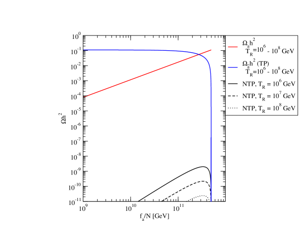
Figure 5.2: Abundance of TP and NTP axino DM and vacuum-misalignment production of axion CDM versus $f_{a}/N$, for various values of $T_{R}$.

In Figure 5.3, we again require $\Omega_{a{\tilde{a}}}h^{2}=0.11$ for HCAMSB benchmark point 1, but this time plot the value of $T_{R}$ which is needed versus $m_{{\tilde{a}}}$, for various values of $f_{a}/N$. The plots terminate at high $T_{R}$ in order to avoid reaching the axion decoupling temperature $T_{a-dcp}$. Dashed curves indicate regions where over 50% of the DM is warm, instead of cold. Solid curves yield the bulk of DM as being cold.
We see that for very light axino masses, and large values of $f_{a}$, the value of $T_{R}$ easily reaches beyond $10^{6}$ GeV, while maintaining the bulk of dark matter as cold. Such high values of $T_{R}$ are good enough to sustain baryogenesis via non-thermal leptogenesis[79], although thermal leptogenesis requires $T_{R}\stackrel{{\scriptstyle>}}{{\sim}}10^{10}$ GeV[40]. Since $f_{a}$ is quite large, we would expect that the dominant portion of DM is composed of relic axions, rather than axinos; as such, detection of the relic axions may be possible at ADMX[3]. While Figures 5.2 and 5.3 were created for the HCAMSB model, quite similar results are obtained for the mAMSB or inoAMSB models.

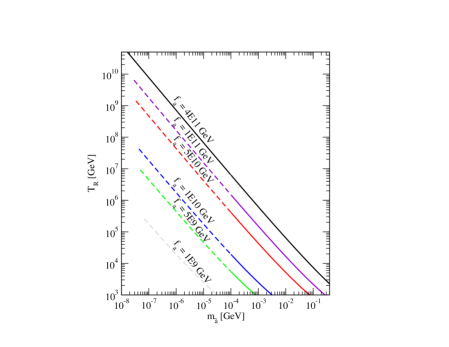
Figure 5.3: Plot of $T_{R}$ needed to ensure $\Omega_{a{\tilde{a}}}h^{2}=0.1$ for HCAMSB benchmark Pt. 1, versus $m_{{\tilde{a}}}$ for various values of the PQ breaking scale $f_{a}$. The dashed curves yield mainly warm axino DM, while solid curves yield mainly cold mixed axion/axino DM.

5.3 Dark Matter Detection

In this section a brief description of Dark Matter experiments are given. These break down into two categories: direct detection (DD) and indirect detection (ID) and each are described separately.

Direct Detection

Direct detections experiments are those that are intended to measure properties of Weakly Interacting Massive Particles (WIMPs) via their direct elastic scatterings off of nuclei. This is in contrast to the ID experiments (described in the next subsection) where WIMP interactions lead to different final state particles, and these products are observed and analyzed.
DD experiments are considered to be extremely important in WIMP searches for a number of reasons. Although a neutralino mass should in principle be re-constructable through LHC data, its interactions are much more difficult to decipher as a result of its inertness in the detector. If there are WIMPS with weak interactions, DD experiments should be able to probe the couplings of these particles. Furthermore, $\not{E}_{T}$ signatures in a collider experiment do not give us information on the stability of particles on cosmological time scales, but only on collider time scales. Thus only DD experiments can tell us whether a particle produced in collisions is “absolutely” stable. And finally, DD experiments do not have the serious systematic uncertainties that ID experiments have. This is because the WIMP properties are measured directly, and because the backgrounds to these experiments are well understood and, in principle, can be controlled. The largest uncertainties in direct detection experiments comes from the observed local density of WIMPs in the vicinity of the earth and their velocity distributions. Increased local density of DM through clumping, etc. would have an impact on the rate of interactions in DD experiments.
Dark matter must be cold and the calculations of wimp-nucleon scattering cross sections must be made in the zero momentum transfer limit. In SUSY theories, the interactions of neutralinos with quarks in the proton are dominated by t-channel CP even Higgs exchange[62]. This is because the relevant vertex is gaugino-higgsino-Higgs [20]. Thus, purely gaugino or purely higgsino neutralinos will have suppressed couplings to nuclei[62].
The total elastic scattering cross section for WIMP-nucleon has contributions from a part that is spin-independent and from one that is spin-dependent. Because the WIMP de Broglie wavelength is expected to be of the order the dimension of heavy atoms, the WIMP will scatter from the coherent composite of nucleons. Thus the spin-independent cross section will be enhanced by factors of $A^{2}$, where A is the atomic number of the target nucleus. The spin- dependent contribution to the cross section only occurs through spin interactions and scales with $J(J+1)$.
The best limits on the spin-dependent cross section come from the Cryogenic Dark Matter Search (CDMS: Ge/Si detectors) experiment which exclude WIMPs with weak scale masses and cross sections at the level of $5\times 10^{-8}$ pb level. We will compare our model to the spin-independent limits set by CDMS and other experiments in the text. We will also compare spin-dependent cross sections as well, but we should note that the constraints placed by spin- dependent DD experiments however are not nearly as strong as for spin- independent cross sections.
The results of the XENON experiments (liquid Xenon detectors) are expected to surpass limits set by its competitors due to its size. XENON has already taken DM searches from the 10 to 100 kg-scale detectors. Impressively, future XENON experiments will be at the ton-scale with SI reaches in the $10^{-10}-10^{-11}$ pb range.

Indirect Detection

Indirect detection (ID) observations are complementary to direct detection (DD) of DM, and there is a wide variety of ID programs that seek annihilation products of DM particles from displaced sources. Any locus of strong gravitation potential is capable of squeezing WIMPs close enough to interact highly with one another. Examples include the galactic center, dwarf spheroidal galaxies, the Sun, the core of the Earth, and inhomogeneities in WIMP halo profiles. However, different sources will provide different information about DM depending on the strength and distance of the source, the distribution of DM around the source, and on the mass and coupling of the WIMPs. A few general descriptions of potential ID signals are described in this subsection

• Gamma Rays

The galactic center of the Milky Way and dwarf spheroidal galaxies in or near the Milky Way are the most capable of gathering DM because of their large gravitation pull. But these sources are relatively far away and so evidence of WIMP interactions must arrive at Earth unattenuated and undeflected by large magnetic field variations in the galaxy. Because gamma rays do not carry charge and travel in straight lines they retain their spectral information and hence are excellent probes of interactions at far distances.
The gamma ray fluxes produced by annihilations of DM for any structure and at any distance was performed in [32] and analyzed in [98]. The expression for the flux of gamma rays is

$$\Phi_{\gamma}(E_{\gamma})\approx 2.8\times 10^{-12}\rm{cm^{-2}s^{-1}}\frac{dN_{\gamma}}{dE_{\gamma}}\biggl{(}\frac{<\sigma v>}{3\times 10^{-26}cm^{2}/s}\biggr{)}\biggl{(}\frac{1\ \rm{TeV}}{m_{\chi}}\biggr{)}^{2}J(\Delta\Omega,\psi)\Delta\Omega,$$ (5.7)

where $\Delta\Omega$ is the solid angle observed and the interaction cross section appears explicitly and $\frac{dN_{\gamma}}{dE_{\gamma}}$ is the spectrum. $J(\Delta\Omega,\psi)$ depends only on the DM distribution and is averaged over the solid angle to give

$$J(\psi)=\frac{1}{8.5\rm{kpc}}\biggl{(}\frac{1}{.3\rm{GeV/cm^{3}}}\biggr{)}^{2}\int_{los}\rho^{2}(r(l,\psi))dl,$$ (5.8)

where the DM density, $\rho$, appears quadratically, $\psi$ is the angle from the galactic center, and the integral takes place over the line of sight (los).
The spectrum for standard astrophysical sources is generally expected to have power law behavior [34], i.e. $\frac{dN_{\gamma}}{dE_{\gamma}}\propto E_{\gamma}^{-\alpha}$. The HESS collaboration has found a high energy source of gamma rays near the galactic center [4] that exhibits the power law behavior with $\alpha=2.2\pm 0.09\pm 0.05$ above the threshold 165 GeV. It is difficult to pick out a signal of DM annihilations from this background, but it is still an interesting target for Fermi-LAT that explores $E_{\gamma}>1$ GeV, which is well below the high HESS energy threshold.

• Antimatter

Charged matter including positrons ($e^{+}$), antiprotons ($\bar{p}$), and antideuterons ($\bar{D}$) are also interesting probes of DM and are produced in WIMP pair-annihilations in the halo. In the case of $wino$ DM pairs will annihilate most efficiently to combinations of Higgs and gauge bosons, whose further decays lead to antimatter [62]. Of these products, cosmic positrons are the most interesting. Because positrons lose the majority their energy over kiloparsec lengths, they only probe the local DM (in sharp contrast to gamma rays). Since DM densities are better understood locally than, say, at the galactic center, positron measurements are subject to fewer systematic uncertainties than other antimatter species.
Cosmic ray protons interacting with our galaxy’s interstellar gas would provide the largest background sources of $\bar{D}$ and $\bar{p}$ fluxes. These types of reactions rarely produce low-energy particles, much less nucleons with energies small enough to match the binding energy of $\bar{D}$ (2.2 MeV) [49]. $\bar{D}$ production is indeed very rare and the background of these particles is highly suppressed at low energies, with estimated flux of $\Phi_{\bar{D}}\sim 5\times 10^{-13}$ [GeV cm² s sr]^-1. For the future GAPS[54] experiment, sensitive to fluxes above $1.5\times 10^{-11}$ [GeV cm² s sr]^-1, the background is essentially absent [45]. An anomalous amount of detected low-energy $\bar{D}$ could be a signature of neutralino annihilations in the halo, because the hadronization of WIMP hadronic annihilation channels (${\tilde{Z}}_{1}{\tilde{Z}}_{1}\rightarrow q\bar{q}$) are confined by color to occur in the rest frame of the halo. Vector boson and Higgs channels can also inject significant amounts of $\bar{D}$ for light Higgs and lower values of WIMP mass [45], especially near the $\bar{D}$ threshold.
Antiproton production is not rare, in contrast to $\bar{D}$, but it also would not be a clean signal of WIMP annihilation at low energies. This is because, of the two, $\bar{p}$ is more susceptible to ionization losses, synchrotron radiation, and solar modulation, allowing it to eventually populate the lower energies [49].

• Neutrinos

WIMPs are thought to become captured by elastically scattering from hydrogen and helium in the Sun and dissipating energy. High-energy neutrinos may be produced in WIMP annihilations in the core of the Sun. The $\nu_{\mu}$s can then undergo $\nu_{\mu}+q\rightarrow q^{\prime}+\mu$ scattering to produce muons in terrestrial ice or water. Thus, the detection of muons on Earth from the WIMP annihilation to neutrinos depends critically on the Sun capture rate of WIMPs, which further depends on the WIMP’s nucleon cross section, its density near the Sun, and its mass.
The the capture rate depends on the effective WIMP-nucleus cross section which is

$$\sigma_{eff}=\sigma_{H}^{SD}+\sigma_{H}^{SI}+0.07\sigma_{He}^{SI},$$ (5.9)

where the factor 0.07 reflects the relative abundance if He to H along with other dynamical factors [62]. An important point here is that while spin-independent WIMP-nucleus cross sections tend to be highly constrained by DD experiments, SD cross sections are not so constrained and can be conceivable much higher. Thus ID experiments such as ICECUBE should be able to probe much lower values of the spin-dependent cross section than DD experiments such as COUPP.

5.4 Direct Detection Rates for the AMSB Models

The ability to directly detect WIMPs depends not only on the mass, interactions, and the local density of the candidate, but also on the local velocity distribution. In the standard cosmological scenario WIMPs are thermally produced in an expanding universe, they freeze out, and then fall into gravitational wells. It is generally assumed, at present, that WIMPs conform to a Maxwell-Boltzmann velocity distribution, $i.e.$, $\ f(v)\sim v^{2}e^{-v^{2}/v_{0}^{2}}$, where $v_{0}^{2}\sim 220$ km/s is the Sun’s velocity about the galactic center. The same distribution holds for our cases, even despite the fact that $non-thermal$ production of the DM candidates (moduli, gravitino, axino decays) can distort the initial velocity distributions of the WIMPs. This is because the original velocity distributions are red-shifted away, and the Maxwell-Boltzmann distributions arise as usual from gravitational in-fall. Thus, the calculations or WIMP-target scattering cross sections for direct detection can be carried out as usual.
As described in Section 5.3, WIMP scattering cross sections from target nuclei are described through spin-independent (SI) and spin-dependent (SD) parts. Because SI cross sections receive enhancement from the mass of heavy targets DD will have better constraints of SI interactions. The SI WIMP-nucleon cross sections are calculated using the Isatools subroutine IsaReS [19].
In Figure 5.4 we scan over all parameters of the mAMSB, HCASMB, and inoAMSBparameter spaces, with a low and high value of $\textrm{tan}\ \beta$ and $\mu>0$, and plot the ${\tilde{Z}}_{1}-p$ scattering cross section versus $m_{{\tilde{Z}}_{1}}$. Only points with $m_{{\tilde{W}}_{1}}>91.9$ GeV are retained, as required by LEP2 [80]. The inoAMSBpoints appear as lines because they have one less parameter than either of the mAMSB or HCAMSB models.
Several crucial features emerge from this plot.

• First, we note that for a given value of $m_{{\tilde{Z}}_{1}}$, the value of $\sigma({\tilde{Z}}_{1}p)$ is bounded from below, unlike the case of the mSUGRA model. That means that wino-WIMP dark matter can be either detected or excluded for a given $m_{{\tilde{Z}}_{1}}$ value.

• Second, we note that the cross section values generally fall in the range that is detectable at present or future DD experiments. The purple contour, for instance, exhibits the CDMS reach based on 2004-2009 data, and already excludes some points, especially those at large $\textrm{tan}\ \beta$. We also show the reach of Xenon-100, LUX, Xenon-100 upgrade, and Xenon 1 ton[53]. These experiments should be able to either discover or exclude AMSB models with $m_{{\tilde{Z}}_{1}}$ values below $\sim 90,\ 100,\ 200$ and 500 GeV respectively. These WIMP masses correspond to values of $m_{{\tilde{g}}}\sim 690,\ 770,\ 1540$ and 3850 GeV, respectively! The latter reach far exceeds the 100 fb^-1 of integrated luminosity reach of LHC for $m_{{\tilde{g}}}$, which were shown in Chapters 3 and 4 to be $m_{{\tilde{g}}}\sim 2.2-2.4$ for HCAMSBand $m_{{\tilde{g}}}<2.6$ TeV for inoAMSBrespectively. For inoAMSB models, where the minimal value of $\sigma^{SI}({\tilde{Z}}_{1}p)$ exceeds that of mAMSB or HCAMSB for a given $m_{{\tilde{Z}}_{1}}$ value, the Xenon 1 ton reach is to $m_{{\tilde{Z}}_{1}}\sim 800$ GeV, corresponding to a reach in $m_{{\tilde{g}}}$ of 6200 GeV!

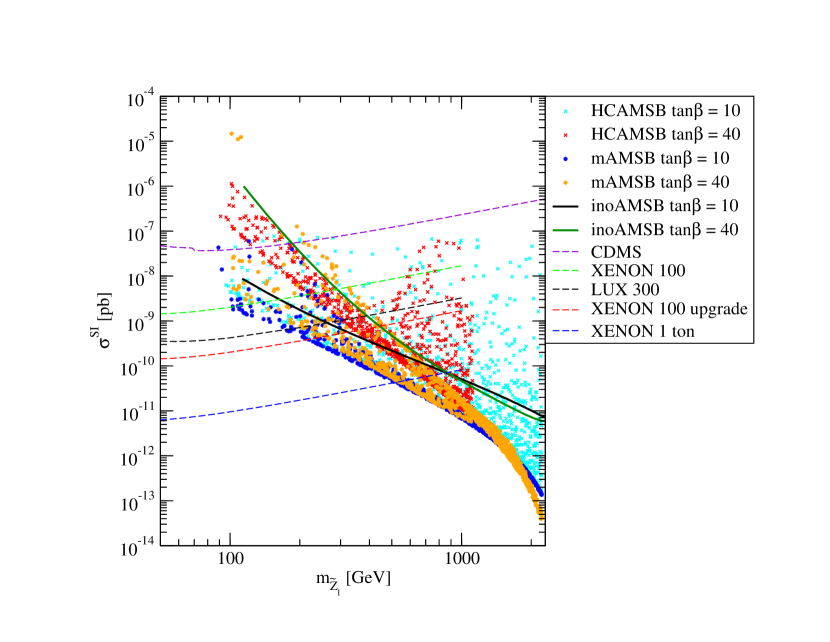
Figure 5.4: Spin-independent ${\tilde{Z}}_{1}-p$ scattering cross section versus $m_{{\tilde{Z}}_{1}}$ for mAMSB, HCAMSB and inoAMSB models for $\textrm{tan}\ \beta=10$ and 40 and $\mu>0$. The parameters $m_{3/2}$ and also $m_{0}$ (for mAMSB) and $\alpha$ (for HCAMSB) have been scanned over. We also show the CDMS limit and projected Xenon and LUX sensitivities.

In Figure 5.5 we scan the parameter spaces again and plot the spin-dependent DD cross section versus $m_{{\tilde{Z}}_{1}}$. The recent DD limit by the COUPP experiment appears at least two orders of magnitude above the theory predictions of all of the models. The probes of the SD cross section are actually better constrained by ID experiments. The ID limits from ICECUBE and its projected DeepCore limit are shown in this figure, and the cross section is that of winos interacting with solar Hydrogen. Though DeepCore will be able to access portions of parameter space, it will not be capable of reaching any of the the models’ lower limits.

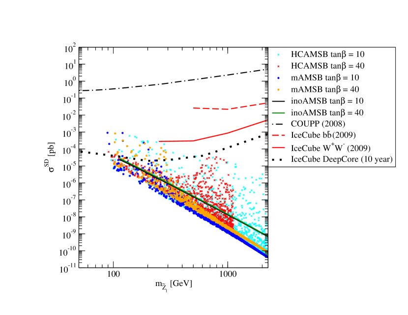
Figure 5.5: Spin-dependent ${\tilde{Z}}_{1}-p$ scattering cross section versus $m_{{\tilde{Z}}_{1}}$ for mAMSB, HCAMSB and inoAMSB models for $\textrm{tan}\ \beta=10$ and 40 and $\mu>0$. The parameters $m_{3/2}$ and also $m_{0}$ (for mAMSB) and $\alpha$ (for HCAMSB) have been scanned over. We also show the COUPP and IceCube limits in $\sigma^{SD}({\tilde{Z}}_{1}p)$.

5.5 Indirect Detection Rates for the AMSB Models

In this section the Indirect Detection (ID) rates for mAMSB, HCAMSB, and inoAMSBare given. We consider the indirect detection of WIMPs from their annihilation in the solar core via neutrino telescopes, and we also consider gamma ray and antimatter fluxes originating in halo WIMP annihilations. These fluxes depend (quadratically) on the assumed density profile of the galaxy, and the results of two profiles, isothermal and Navarro-Frenk-White [86], are given. Most halo models are in near-agreement at the Earth’s position ($\sim$ 8 kpc from the galactic center), however they differ widely at the inner parsecs of the galaxy. This translates into large uncertainties in the gamma fluxes from these regions. As mentioned in Section 5.3, antimatter signals tend to have fewer uncertainties because they should originate closer to earth.
This section is broken into three parts. In the first subsection we consider the mAMSBmodel and calculate ID rates by varying $m_{0}$ and $\textrm{tan}\ \beta$ and analyze the interactions that lead to these rates. In the following subsection we do the same for HCAMSB, but this time we vary $\alpha$ and $\textrm{tan}\ \beta$. And finally, in the last subsection we show the calculated ID rates while varying the remaining parameter, $m_{3/2}$, for the mAMSB, HCAMSB, and the inoAMSBmodels.

Indirect Wino Detection for mAMSB

We begin the analysis with mAMSB. We choose $m_{3/2}=$ 50 TeV and $\textrm{tan}\ \beta=10$, which gives a wino-like neutralino with mass $m_{{\tilde{Z}}_{1}}\simeq 144$ GeV. All of the ID rates for these parameters, while varying $m_{0}$, are shown in Figure 5.6 and each is discussed in turn.
In Figure 5.6 (a) we show the SI DD cross section for comparison, along with approximate reaches for XENON-10 and XENON-100. For higher $m_{0}$, the value of $|\mu|$ drops, much like it does in mSUGRA when the focus-point region is approached. Thus, when $m_{0}$ is large, ${\tilde{Z}}_{1}$ picks up a higgsino component that enhances the SI DD cross section since the relevant vertex is Higgs-higgsino-gaugino. For $m_{0}\stackrel{{\scriptstyle>}}{{\sim}}3500$ GeV, it is seen that the ${\tilde{Z}}_{1}$ becomes directly observable for XENON-100.
Figure 5.6 (b) shows the first ID rate which is the flux of muons from the solar direction. To calculate the flux we used the Isajet/DarkSusy interface (see Chapter 1 for descriptions of these programs) and require $E_{\mu}>50$ GeV as required for ICECUBE. When ${\tilde{Z}}_{1}$s annihilate in the core of the Sun they produce $\nu_{\mu}$s that travel to Earth and convert in water/ice to muons via the charged-current interaction. ${\tilde{Z}}_{1}$s are captured by the Sun in the first place through its spin-dependent interactions with Hydrogen that is mainly sensitive to $Z^{*}$ exchange. Thus, for larger values of $m_{0}$ where the neutralino has more higgsino content, the flux is expected to be larger due to the $Z$-${\tilde{Z}}_{1}$-${\tilde{Z}}_{1}$ coupling.
In Figure 5.6 (c) we show the expected flux of gamma rays from the galactic core with $E_{\gamma}>1$ GeV as required by the Fermi Gamma-ray Space Telescope (FGST) experiment. The gamma ray fluxes are due to neutralino annihilations and depend mainly on the ${\tilde{Z}}_{1}{\tilde{Z}}_{1}\rightarrow W^{+}W^{-}$ annihilation cross section which occurs via chargino exchange. This is followed by $W\rightarrow q\bar{q}^{\prime}\rightarrow$ $\ \pi^{0}\rightarrow\gamma\gamma$ to produce the gammas. The rates do not change with $m_{0}$ because ${\tilde{Z}}_{1}$s remain wino-like and the chargino mass does not change significantly. As expected, the type of profile plays a significant role in gamma detection, and the predictions for the two differ by over an order of magnitude. Still, in both cases the fluxes exceed the approximate reach of FGST.
Figures 5.6 (d)-(f) show antimatter fluxes for $e^{+}$, $\bar{p}$, and $\bar{D}$ respectively that come from halo annihilations. For $e^{+}$ and $\bar{p}$ there are observable rates predicted for Pamela [89], and $\bar{D}$ observables rates might be seen by GAPS [54]. These elevated rates reflect the $wino-wino$ annihilation into $W^{+}W^{-}$ cross section.

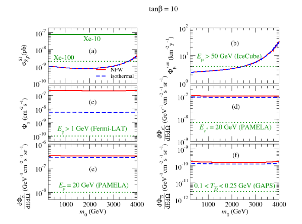
Figure 5.6: Wino CDM direct detection (a) and indirect detection (b)–(f) rates versus $m_{0}$ in mAMSB for $m_{3/2}=50$ TeV, $\textrm{tan}\ \beta$=10, and $\mu>0$.

Now the same calculations are done and plotted in Figure 5.7 with $m_{3/2}=50$ TeV and $\mu>0$, but this time $\textrm{tan}\ \beta$ is increased 40. The SI DD cross section in frame (a) has the usual enhancement due to increased higgsino content of ${\tilde{Z}}_{1}$ at larger $m_{0}$ values. Additionally, there is an enhancement for low $m_{0}$ values as well. As described in Section 5.3, $\sigma^{SI}_{{\tilde{Z}}_{1}p}$ depends on Higgs and squark exchange diagrams between ${\tilde{Z}}_{1}$ and quarks and through loops via Higgs exchange between ${\tilde{Z}}_{1}$ and gluons. Now that $\textrm{tan}\ \beta$ is higher, the heavy Higgs mass is quite light, e.g., for $m_{0}\sim$ 600 GeV the heavy Higgs mass is $m_{H}\sim$ 152 GeV. This results in a huge DD cross section at low $m_{0}$, and regions with $m_{0}\stackrel{{\scriptstyle<}}{{\sim}}900$ GeV and $\textrm{tan}\ \beta=40$ are already excluded by DD WIMP searches.
Related to this, Figure 5.7 (b) shows an increase in the muon flux for low $m_{0}$ and $\textrm{tan}\ \beta=40$. Usually the spin-dependent cross section is considered to be the most important part of ${\tilde{Z}}_{1}$ capture at high $\textrm{tan}\ \beta$ in the sun because the SI cross section receives minimal enhancement from the target (H and He) masses. However, because of the lighter Higgs effects of the last paragraph at low $m_{0}$, the SI cross section plays a significant role in ${\tilde{Z}}_{1}$ capture and hence muon detection on Earth. Of course, this region is already excluded by DD experiments. We also note the interesting “anti-resonance” effect in $\Phi_{\mu}$ for $m_{0}\sim 850$ GeV. Here, $m_{A}\sim 2m_{{\tilde{Z}}_{1}}$, and on the Higgs resonance ${\tilde{Z}}_{1}{\tilde{Z}}_{1}\rightarrow b\bar{b}$ is the dominant annihilation mode. The $b$-decays modes produce a softer distribution of $\nu_{\mu}$s than from vector bosons leading to fewer muons passing the $E_{\mu}>50$ GeV requirement, and hence the sharp dip in flux. Finally, at large $m_{0}$ we again see an increase in muon flux due to the increased higgsino component of ${\tilde{Z}}_{1}$.
Finally, gamma and antimatter fluxes versus $m_{0}$ are shown in Figure 5.7 in frames (c) - (f). The rates are again flat due to the constant ${\tilde{Z}}_{1}{\tilde{Z}}_{1}$ annihilation rate to vector bosons. The exception occurs at $m_{0}\sim 850$ GeV where the $A$-resonance enhances the annihilation rate [18]. At high $m_{0}$, $e^{+}$ and $\bar{p}$ fluxes drop slightly because ${\tilde{Z}}_{1}{\tilde{Z}}_{1}$ annihilations to $b\bar{b}$ become prominent relative to the usual vector boson products. Subsequent decays lead to softer $e^{+}$ and $\bar{p}$, and hence less detectability above the $E_{e^{+},\bar{p}}=20$ GeV threshold. In frame (f), the $\bar{D}$ rate actually increases with $m_{0}$ since the softer $\bar{D}$s produced are still in the low energy range of detection.

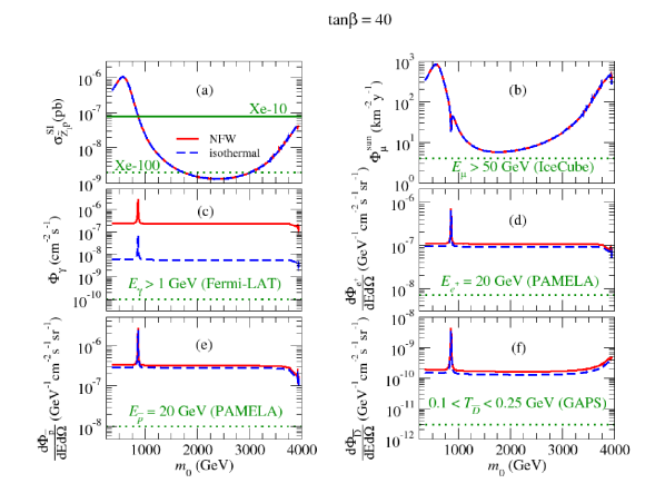
Figure 5.7: Wino CDM direct detection (a) and indirect detection (b)–(f) rates versus $m_{0}$ in mAMSB for $m_{3/2}=50$ TeV, $\textrm{tan}\ \beta$=40, and $\mu>0$.

Indirect Wino Detection for HCAMSB

In this subsection results similar to those of the last subsection are shown for the HCAMSBmodel for $m_{3/2}=50$ TeV, but now we vary the $\alpha$ parameter. It was seen in Chapter 3 that $\alpha\sim 0$ corresponds to pure anomaly mediation, while larger $\alpha$ values give increasing $M_{1}$ at the GUT scale. This affects the RGEs of sparticle masses through their hypercharge numbers, and this leads to a left-right split sparticle spectrum at the weak scale. This effect, combined with the effect of a large t-quark Yukawa coupling, leads to light, dominantly left top squark state ${\tilde{t}}_{1}$ at large $\alpha$. Raising $\alpha$ also leads to a diminished $|\mu|$ value, and this results in ${\tilde{Z}}_{1}$ acquiring more of a higgsino component.
Figure 5.8 (a) shows the SI cross section for direct detection. Reminiscent of $m_{0}$ in mAMSB, the cross section increases for larger values of $\alpha$, and this is, of course, due to the larger higgsino component of ${\tilde{Z}}_{1}$.
In Figure 5.8 (b) is the muon flux versus $\alpha$ for the HCAMSBmodel. At low $\alpha$ the flux is quite low, but increases considerable at high $\alpha$. The higgsino component at high $\alpha$ leads to unsuppressed couplings to $Z$. Since the ${\tilde{Z}}_{1}$–nucleon SD cross section, is mainly sensitive to $Z^{*}$-exchange, a higher flux of muons are seen on the Earth.
In Figure 5.8, in frames (c)-(f) are the plots of the gamma ray flux and antimatter fluxes. The high rates are due to the large $wino-wino$ $\rightarrow VV$ annihilation cross sections and are relatively flat with $\alpha$. At large $\alpha$ the annihilation to $b\bar{b}$ states is enhanced leading to smaller detection rates for $e^{+}$ and $\bar{p}$ (softer spectrum does not pass experimental threshold) and slightly increased $\bar{D}$ (by soft energy requirements).

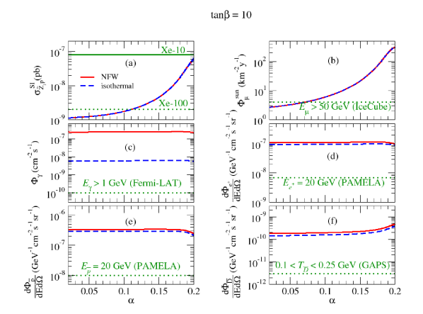
Figure 5.8: Wino CDM direct detection (a) and indirect detection (b)–(f) rates versus $\alpha$ in HCAMSBfor $m_{3/2}=50$ TeV, $\textrm{tan}\ \beta$=0, and $\mu>0$.

In Figure 5.9, we perform the same calculations as in Figure 5.8, but now $\textrm{tan}\ \beta$ is chosen to be 40. In frame (a), the spin-independent DD cross section is enhanced relative to the $\textrm{tan}\ \beta=10$ case because of the now much lighter, heavy and pseudoscalar Higgs ($H$ and $A$) and the increased $b$-quark Yukawa coupling. As $\alpha$ increases, $m_{H}$ increases and the rate diminishes until the highest $\alpha$ values are reached. Here the presence of the higgsino component of ${\tilde{Z}}_{1}$ enhances the cross section. As in the mAMSBcase, the large SI enhancement leads to greater solar capture rate of ${\tilde{Z}}_{1}$s, which in turn leads to greater muon fluxes on earth, and this is seen in frame (b).
In Figure 5.9 (b), we see the same type of anti-resonance effect as in Figure 5.7, where near $2m_{{\tilde{Z}}_{1}}\sim m_{A}$, annihilation to heavy fermion pairs dominate over the usual $VV$ pairs ($V=W^{\pm},\ Z$), and lead to a softer distribution of neutrinos. In frames (c)-(f) are the halo annihilation rates for HCAMSBwith $\textrm{tan}\ \beta=40$. These rates are generally flat with changing $\alpha$, and do not suffer an increase as compared with low $\textrm{tan}\ \beta$, since $wino-wino\rightarrow VV$ still dominates the annihilation rate. The exception again occurs near the A-resonance, and halo annihilation is enhanced by pseudoscalar Higgs exchange.

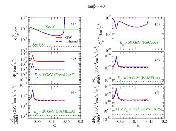
Figure 5.9: Wino CDM direct detection (a) and indirect detection (b)–(f) rates versus $\alpha$ in HCAMSBfor $m_{3/2}=50$ TeV, $\textrm{tan}\ \beta$=40, and $\mu>0$.

Indirect Detection Rates for mAMSB, HCAMSB, and inoAMSBversus $m_{3/2}$

In this subsection we explore the remaining parameter of our AMSB models: $m_{3/2}$. While $m_{3/2}$ is roughly bounded from below by LEP2 constraints, in principle there is no upper bound for the parameter. In general, increasing the gravitino mass increases all sparticle mass as can be seen for example in Table 4.1 for the inoAMSBcase. Thus we expect a diminution of rates toward higher $m_{3/2}$ values due to decreased interactions. Also, in all ID plots we assume the standard NFW halo profile.
In Figure 5.10 we show direct and indirect wino DM detection rates versus $m_{3/2}$ for all three models considered in this thesis, with $\textrm{tan}\ \beta=10$ and $\mu>0$. For the comparison, in the HCAMSBcase the choice $\alpha=0.1$ is made, and for mAMSBwe take $m_{0}=1$ TeV.
The spin-independent cross section is shown in frame (a) of Figure 5.10 for all models. The larger inoAMSBcross section is due in part to the smaller $\mu$ values for a given $m_{3/2}$, which enhances ${\tilde{Z}}_{1}$ scattering via Higgs exchange made possible by the Higgs-higgsino-gaugino vertex.
Figure 5.10 (b) shows the muon flux with the minimum energy of $E_{\mu}>50$ GeV required for detectability at IceCube. Due to the relative values of $\mu$ in all three models, inoAMSByields the highest rates while mAMSByields the lowest. Since inoAMSBgenerally has the lowest $|\mu|$ values, its ${\tilde{Z}}_{1}$ can interact more strongly through $Z^{*}$ exchange (see previous two subsections). This enhances the SD cross section, which eventually leads to greater $\mu$ flux on earth. The rough reach of IceCube is shown, and the figure indicates that the lower values of $m_{3/2}$ may be accessible in $\nu_{\mu}\rightarrow\mu$ searches.
The ID rates for $\gamma$,$e^{+}$,$\bar{p}$, and $\bar{D}$ are shown in Figure 5.10, frames (c)-(f). The rates for all models are nearly identical in each case for varying $m_{3/2}$. This is due to the dominance of ${\tilde{Z}}_{1}{\tilde{Z}}_{1}$$\rightarrow VV$ halo annihilations, which mainly depend on the gaugino (wino) component of ${\tilde{Z}}_{1}$. Rough reaches for Fermi-LAT, Pamela, and GAPS are shown for reference, and high wino annihilations should yield observable signals.

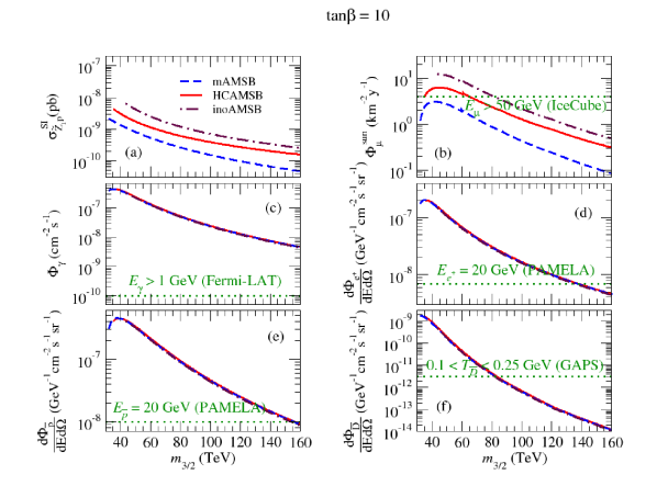
Figure 5.10: DD and ID rates for wino CDM in mAMSB, HCAMSB, and inoAMSBmodels versus $m_{3/2}$, for $\textrm{tan}\ \beta=10$, and $\mu>0$. For mAMSB, $m_{0}=1$ TeV, and for HCAMSB, $\alpha=0.1$. In these plots we adopt the NFW DM halo profile.

Increasing $\textrm{tan}\ \beta$ to 40, the same rates are shown versus $m_{3/2}$ in Figure 5.11. As in the previous subsections, the SI cross section in frame (a) is enhanced relative to $\textrm{tan}\ \beta=10$ due to the simultaneous decrease in the Higgs mass and increase in $b$-quark Yukawa coupling. Because inoAMSBhas both the smallest $m_{H}$ and smallest $|\mu|$ values of all models for low $m_{3/2}$, this model shows the largest SI cross section. As $m_{3/2}$ increases, $m_{H}$ increases for inoAMSBand HCAMSB, but actually decreases for mAMSB. Thus for $m_{3/2}\stackrel{{\scriptstyle>}}{{\sim}}75$ TeV, the mAMSBmodel yields the highest value of $\sigma^{SI}({\tilde{Z}}_{1}p)$.
Figure 5.11, frame (b), shows the muon flux, which is elevated relative to the $\textrm{tan}\ \beta=10$ case, again due to the increased SI cross section of frame (a). At low $m_{3/2}$ the inoAMSBmodel shows the highest flux due to its low $\mu$ value which enhances the $Z^{*}$ exchange in ${\tilde{Z}}_{1}$-$q$ scattering. Around $m_{3/2}\sim 60$ TeV, the mass of A is near twice the ${\tilde{Z}}_{1}$ mass, and resonant ${\tilde{Z}}_{1}$ annihilations to $b\bar{b}$ final states dominate over $VV$. This diminishes the flux of detectable muons (see previous two subsections for further discussion). For higher $m_{3/2}$ values, beyond the resonance, the $mAMSB$ model yields the highest muon flux due to its elevated value of $\sigma^{SI}({\tilde{Z}}_{1}p)$.
Figure 5.11, frames (c)-(f), show the gamma and antimatter fluxes versus $m_{3/2}$. Relatively little change in the ID rates are seen in going from $\textrm{tan}\ \beta=10$ to $\textrm{tan}\ \beta=40$, since $wino-wino\rightarrow VV$ dominates the annihilations. An exception, of course, is due to A-resonance enhancement of halo annihilations, where $2m_{{\tilde{Z}}_{1}}\sim m_{A}$. And $\bar{D}$ rates appear enhanced for inoAMSBand mAMSBat large $m_{3/2}$ because in these cases the ${\tilde{Z}}_{1}{\tilde{Z}}_{1}$$\rightarrow$$b\bar{b}$ annihilation rate, which does receive $\textrm{tan}\ \beta$ enhancement, contributes to the detection of rather low energy $\bar{D}$s.

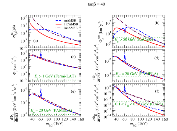
Figure 5.11: DD and ID rates for wino CDM in mAMSB, HCAMSB, and inoAMSBmodels versus $m_{3/2}$, for $\textrm{tan}\ \beta=40$, and $\mu>0$. For mAMSB, $m_{0}=1$ TeV, and for HCAMSB, $\alpha=0.1$. In these plots we adopt the NFW DM halo profile.

5.6 Summary

In this Chapter we have investigated aspects of cold dark matter in three models of anomaly mediation: mAMSB, HCAMSB and inoAMSB. Typically, each gives rise to a wino-like lightest neutralino, unless very high values of $m_{0}$ (for mAMSB) or $\alpha$ (for HCAMSB) are used, in which case the ${\tilde{Z}}_{1}$ becomes a mixed wino-higgsino state. In this class of models with a wino-like ${\tilde{Z}}_{1}$, the thermal abundance of neutralino CDM is well below measured values, unless $m_{{\tilde{Z}}_{1}}\stackrel{{\scriptstyle>}}{{\sim}}1300$ GeV. We discuss four ways to reconcile the predicted abundance of CDM with experiment:

1. enhanced neutralino production via scalar field (e.g. moduli) decay,

2. enhanced neutralino production via gravitino decay, where gravitinos may arise thermally, or by moduli or inflaton decay,

3. enhanced neutralino production via heavy axino decay, and

4. neutralino decay to axinos, where the bulk of CDM comes from a mixture of vacuum mis-alignment produced axions and thermally produced axinos.

Cases 1 and 2 should lead to a situation where all of CDM is comprised of wino- like WIMPs; they will be very hard, perhaps impossible, to tell apart. Case 3 would contain a mixture of axion and wino-like WIMP CDM. It is a scenario where it is possible that both a WIMP and an axion could be detected. Case 4 predicts no direct or indirect detection of WIMPs, but a possible detection of relic axions. It is important to note that more than one of these mechanisms may occur at once: for instance, we may gain additional neutralino production in the early universe from moduli, gravitino and axino decay all together.
In Sections 5.4 and 5.5, we presented rates for direct and indirect detection of relic wino-like WIMPs. The SI direct detection cross sections are bounded from below. Ultimately, ton-scale noble liquid or SuperCDMS experiments should probe out to $m_{{\tilde{Z}}_{1}}\sim 500$ GeV, which would exceed the 100 ${\textrm{fb}^{-1}}$ reach of LHC; a non-observation of signal would put enormous stress on AMSB-like models as new physics. We also evaluated SD direct detection: current experiments have little reach for AMSB-like models, although IceCube DeepCore and possibly COUPP upgrades may probe more deeply.
WIMP indirect detection rates for all three AMSB models were also presented. The IceCube experiment has some reach for WIMPs from AMSB models, especially at high $\textrm{tan}\ \beta$ or when the ${\tilde{Z}}_{1}$ picks up a higgsino component. We noted an interesting inverse resonance effect in the muon flux detection rate, caused by transition from solar core annihilations to $VV$ states, to annihilations to mainly $b\bar{b}$ states. The detection of $\gamma$s, $e^{+}$s, $\bar{p}$s and $\bar{D}$s are all elevated in AMSB-like models compared to mSUGRA [18], due to the high rate for ${\tilde{Z}}_{1}{\tilde{Z}}_{1}\to VV$ annihilation in the galactic halo. The results do depend on the assumed halo profile, especially for $\gamma$ ray detection in the direction of the galactic core. Generally, if a signal is seen in the $e^{+}$ channel, then one ought to be seen in the $\bar{p}$ channel, and ultimately in the $\gamma$, $\bar{D}$ (if/when GAPS flies) or direct detection channel. In addition, a sparticle production signal should ultimately be seen at the LHC, at least for $m_{{\tilde{g}}}\stackrel{{\scriptstyle<}}{{\sim}}2400$ GeV, once 100 ${\textrm{fb}^{-1}}$ of integrated luminosity is accrued.
As a final remark, we should note here that the dark matter detection signals all provide complementary information to that which will be provided by the CERN LHC. At the LHC, each model– mAMSB, HCAMSB and inoAMSB– will provide a rich assortment of gluino and squark cascade decay signals which will include multi-jet plus multi-lepton plus missing $E_{T}$ events. In all cases, the wino-like lightest neutralino state will be signaled by the well-known presence of highly ionizing tracks (HITs) from quasi-stable charginos with track length of order centimeters, before they decay to soft pions plus a ${\tilde{Z}}_{1}$. It was discussed in Chapter 4 that the three models should be distinguishable at the LHC by the differing opposite-sign/same flavor dilepton invariant mass distributions. In the case of mAMSB, with $m_{{\tilde{l}}_{L}}\simeq m_{{\tilde{l}}_{R}}$, we expect a single mass edge from ${\tilde{Z}}_{2}\to$ $l{\tilde{l}}_{L,R}\to$ $l^{+}l^{-}{\tilde{Z}}_{1}$ decay. In HCAMSB, the sleptons are rather heavy, and instead ${\tilde{Z}}_{2}\to{\tilde{Z}}_{1}Z$ occurs at a large rate, leading to a bump in $m(l^{+}l^{-})\sim M_{Z}$, upon a continuum distribution. In inoAMSB, with $m_{{\tilde{Z}}_{2}}>m_{{\tilde{l}}_{L,R}}$, but with ${\tilde{l}}_{L}$ and ${\tilde{l}}_{R}$ split in mass (due to different $U(1)_{Y}$ quantum numbers), a characteristic double mass edge is expected in the $m(l^{+}l^{-})$ invariant mass distribution.

6 Conclusion

We conclude by summarizing the main points of this thesis. We have compared three model types, all having supergravity anomaly contributions (AMSB) to the soft parameters. We began with the mAMSBmodel of Chapter 2 which was the starting point of comparison for all other models. This model features a wino-like LSP (${\tilde{Z}}_{1}$), a lightest chargino (${\tilde{W}}_{1}$) with mass nearly equal to that of the LSP, and a near left-right degeneracy in scalar masses. Since $m_{{\tilde{Z}}_{1}}\sim m_{{\tilde{W}}_{1}}$, we expect the presence of HITs (for all of the models) as described in Chapter 2. The second lightest neutralino, ${\tilde{Z}}_{2}$, is bino-like and can be produced in LHC pp collisions and subsequently decays through ${\tilde{Z}}_{2}\rightarrow{\tilde{l}}_{L/R}^{\pm}l$, while slepton decays produce the LSP and dilepton final states. Since left- and right-handed states are degenerate, the OS $m(l^{\pm}l^{\mp})$ distribution for these final states results in a single (comparatively large) mass edge, as can be see in Figure 4.12.
We also examined the Hypercharged Anomaly Mediated Supersymmetry-Breaking model, which incorporates effects from a geometrically separated hidden sector. The hidden sector communicates the supersymmetry-breaking to the visible sector via a combination of supergravity anomaly and a new $U(1)$ mediation. The soft masses are those of mAMSB, but with an extra contribution to the bino mass parameterized as $\alpha$ in Equation (3.12). Because left- and right-handed particles have different hypercharge quantum numbers, the mass spectrum for this model is highly left-right split (in contrast to mAMSB). The LSP is still a wino-like neutralino with near-degeneracy to the lightest chargino, and we again expect highly-ionizing track chargino events. The second-lightest neutralino, however, is higgsino-like in this case due to heaviness of the bino soft mass, $M_{1}$. The higgsino component in ${\tilde{Z}}_{2}$ allows for decays to $Z$ and ${\tilde{Z}}_{1}$. Without intermediate slepton decays, the OS dilepton distribution appears as a smooth distribution with a peak around $m_{Z}$.
The last model(s) we examined originate in string theories with Calabi-Yao orientifold compactifications and moduli stabilization through fluxes and non-perturbative (KKLT) effects. The supersymmetry-breaking is communicated to the MSSM via gravitation. The resulting soft contributions appear as a combination of anomaly mediation and gaugino mediation, and we have labeled these parameters space points “inoAMSB”. In these models, the AMSB contributions are only present for gaugino masses, $M_{1},M_{2}$, and $M_{3}$. But like gaugino mediation, the soft scalar and trilinear coupling are suppressed, $i.e.$, $m_{0}\sim A_{0}\sim 0$ at $M_{string}$. We expect for this class of models to yield HITs, as usual for AMSB models. We also expect with a double edge structure in the $m(l^{\pm}l^{\mp})$ distribution. This is because, like in mAMSB, ${\tilde{Z}}_{2}$ is bino-like, but the sleptons here are left-right split leading to two distinct mass edges, instead of just one as in the mAMSB framework (again, see Figure 4.12).
Finally, we explored the Dark Matter predictions for all of these models. It is well-known that the neutralino LSPs of AMSB models annihilate and co-annihilate too efficiently to account for DM relic density of the universe. However, if any of these models are the correct description of nature, there are likely other $non$-$thermal$ sources of LSP-production that can serve to increase the value of the relic density. Assuming these mechanism provide the correct DM abundance, we calculated direct and various indirect detection rates for a multitude of experiments for every model. For the direct detection, we saw that CDMS data has already excluded some regions of the parameters spaces of these models. It was also striking to find that the cross sections were all bounded from below (Figure 5.4), leading to a XENON 1 Ton reach that far exceeded the reach of the LHC; the extreme example being the inoAMSBreach $m_{\tilde{g}}\sim$ 6.2 TeV compared to $m_{\tilde{g}}\stackrel{{\scriptstyle<}}{{\sim}}2.6$ TeV for 100 ${\textrm{fb}^{-1}}$ of LHC data.
For indirect detection, we found that the ICECUBE experiment provided some reach for AMSB models, particularly in cases with high $\textrm{tan}\ \beta$, or in parameter space regions where ${\tilde{Z}}_{1}$ has significant higgsino content (high $m_{0}$ or high $\alpha$). The detection elevated rates of gammas, positrons, antiprotons, and antideuterons in AMSB models is due to high rate of ${\tilde{Z}}_{1}{\tilde{Z}}_{1}\rightarrow VV$ annihilations. We noted interesting inverse resonance effects in the muon flux. We also observed how indirect detection rates depend on the assumed galactic DM profile.

Bibliography

- [1] L. F. Abbott and P. Sikivie, Phys. Lett. B 120 (1983) 133; J. Preskill, M. Wise and F. Wilczek, Phys. Lett. B 120 (1983) 127; M. Dine and W. Fischler, Phys. Lett. B 120 (1983) 137; M. Turner, Phys. Rev. D 33 (1986) 889; L. Visinelli and P. Gondolo, Phys. Rev. D 80 (2009) 035024.
- [2] B. S. Acharya, G. Kane, S. Watson and P. Kumar, Phys. Rev. D 80, 083529 (2009) [arXiv:astro-ph.CO/0908.2430].
- [3] L. Duffy et al., Phys. Rev. Lett. 95 (2005) 091304 and Phys. Rev. D 74 (2006) 012006; for a review, see S. Asztalos, L. Rosenberg, K. van Bibber, P. Sikivie and K. Zioutas, Ann. Rev. Nucl. Part. Sci.56 (2006) 293.
- [4] F. Aharonian et al. [The HESS Collaboration], Astron. Astrophys. 425, L13 (2004) [arXiv:astro-ph/0408145].
- [5] S. P. Ahlen et al., Phys. Lett. B 195 (1987) 603; D. Caldwell et al., Phys. Rev. Lett. 61 (1988) 510 and Phys. Rev. Lett. 65 (1990) 1305; D. Reusser et al., Phys. Lett. B 235 (1991) 143; T. Falk, K. Olive and M. Srednicki, Phys. Lett. B 339 (1994) 248.
- [6] J. Angle et al. [XENON Collaboration], Phys. Rev. Lett. 100, 021303 (2008) [arXiv:astro-ph/0706.0039].
- [7] D. Amati, K. Konishi, Y. Meurice, G. C. Rossi and G. Veneziano, Phys. Rept. 162, 169 (1988).
- [8] C. Amsler et al. [Particle Data Group], Phys. Lett. B 667, 1 (2008).
- [9] N. Arkani-Hamed and H. Murayama, JHEP 0006, 030 (2000) [arXiv:hep-th/9707133].
- [10] T. Asaka, S. Nakamura and M. Yamaguchi, Phys. Rev. D 74, 023520 (2006) [arXiv:hep-ph/0604132].
- [11] For a recent review, see P. Sikivie, hep-ph/0509198; M. Turner, Phys. Rept. 197 (1990) 67; J. E. Kim and G. Carosi, arXiv:0807.3125 (2008)
- [12] H. Baer and C. Chen and F. Paige and X. Tata, “Detecting Sleptons at Hadron Colliders and Supercolliders“ Physical Review D vol. 49 (1994) [arXiv:hep-ph/9311248]
- [13] H. Baer and M. Brhlik, Phys. Rev. D 55, 3201 (1997) [arXiv:hep-ph/9610224];
- [14] H. Baer, M. Brhlik, D. Castano and X. Tata, Phys. Rev. D 58, 015007 (1998) [arXiv:hep-ph/9712305].
- [15] H. Baer, R. B. Munroe and X. Tata, Phys. Rev. D 54, 6735 (1996) [Erratum-ibid. D 56, 4424 (1997)] [arXiv:hep-ph/9606325].
- [16] H. Baer, J. K. Mizukoshi and X. Tata, Phys. Lett. B 488, 367 (2000) [arXiv:hep-ph/0007073].
- [17] H. Baer, C. Balazs, J. Ferrandis and X. Tata, Phys. Rev. D 64, 035004 (2001) [arXiv:hep-ph/0103280].
- [18] H. Baer and J. O’Farrill, JCAP 0404, 005 (2004) [arXiv:hep-ph/0312350]; H. Baer, A. Belyaev, T. Krupovnickas and J. O’Farrill, JCAP 0408, 005 (2004) [arXiv:hep-ph/0405210].
- [19] H. Baer, C. Balazs, A. Belyaev and J. O’Farrill, JCAP 0309, 007 (2003) [arXiv:hep-ph/0305191].
- [20] For detailed discussions see H. Baer and X. Tata, Weak scale supersymmetry: From superfields to scattering events, Cambridge, UK: Univ. Pr. (2006)
- [21] H. Baer, A. Lessa and H. Summy, Phys. Lett. B 674, 49 (2009) [arXiv:hep-ph/0809.4719 ].
- [22] H. Baer, H. Prosper and H. Summy, Phys. Rev. D 77, 055017 (2008) [arXiv:hep-ph/0801.3799].
- [23] H. Baer, V. Barger, A. Lessa and X. Tata, JHEP 0909, 063 (2009) [arXiv:hep-ph/0907.1922].
- [24] H. Baer, A. D. Box and H. Summy, JHEP 0908, 080 (2009) [arXiv:hep-ph/0906.2595].
- [25] H. Baer, R. Dermisek, S. Rajagopalan and H. Summy, JHEP 0910, 078 (2009) [arXiv:hep-ph/0908.4259].
- [26] H. Baer, S. de Alwis, K. Givens, S. Rajagopalan and H. Summy, JHEP 1005, 069 (2010) [arXiv:hep-ph/1002.4633].
- [27] H. Baer, R. Dermisek, S. Rajagopalan and H. Summy, JCAP 1007, 014 (2010) [arXiv:hep-ph/1004.3297].
- [28] V. Balasubramanian, P. Berglund, J. P. Conlon and F. Quevedo, JHEP 0503, 007 (2005) [arXiv:hep-th/0502058].
- [29] E. Barberio et al. [Heavy Flavor Averaging Group (HFAG)], [arXiv:hep-ex/0603003].
- [30] A. J. Barr, C. G. Lester, M. A. Parker, B. C. Allanach and P. Richardson, JHEP 0303, 045 (2003) [arXiv:hep-ph/0208214].
- [31] A. Barr, C. Lester and P. Stephens, J. Phys. G 29, 2343 (2003) [arXiv:hep-ph/0304226].
- [32] L. Bergstrom, J. Edsjo and P. Ullio, Phys. Rev. Lett. 87, 251301 (2001) [arXiv:astro-ph/0105048].
- [33] W. Beenakker, R. Hopker and M. Spira, PROSPINO: A program for the PROduction of Supersymmetric Particles In Next-to-leading Order QCD, [arXiv:hep-ph/9611232].
- [34] G. Bertone, Dark Matter: A Multidisciplinary Approach, [arXiv:astro-ph/0710.5603].
- [35] R. Blumenhagen, S. Moster and E. Plauschinn, JHEP 0801, 058 (2008) [arXiv:hep-th/0711.3389].
- [36] M. Bolz, A. Brandenburg and W. Buchmuller, Nucl. Phys. B 606, 518 (2001) [Erratum-ibid. B 790, 336 (2008)] [arXiv:hep-ph/0012052].
- [37] A. Brandenburg and F. D. Steffen, JCAP 0408, 008 (2004) [arXiv:hep-ph/0405158].
- [38] A. Brignole, L. E. Ibanez and C. Munoz, Soft supersymmetry-breaking terms from supergravity and superstring models, [arXiv:hep-ph/9707209].
- [39] H. N. Brown et al. (Muon g-2 collaboration), Phys. Rev. Lett. 86 (2001) 2227
- [40] W. Buchmuller, P. Di Bari and M. Plumacher, Nucl. Phys. B 643, 367 (2002) [Erratum-ibid. B 793, 362 (2008)] [arXiv:hep-ph/0205349].
- [41] C. H. Chen, M. Drees and J. F. Gunion, Phys. Rev. D 55, 330 (1997) [Erratum-ibid. D 60, 039901 (1999)] [arXiv:hep-ph/9607421].
- [42] C. H. Chen, M. Drees and J. F. Gunion, Addendum/Erratum for Searching for invisible and almost invisible particles at e+ e- colliders and A non-standard string/SUSY scenario and its phenomenological implications,” [arXiv:hep-ph/9902309].
- [43] K. Y. Choi, J. E. Kim, H. M. Lee and O. Seto, Phys. Rev. D 77, 123501 (2008) [arXiv:hep-ph/0801.0491].
- [44] L. Covi, J. E. Kim and L. Roszkowski, Phys. Rev. Lett. 82, 4180 (1999) [arXiv:hep-ph/9905212]; L. Covi, H. B. Kim, J. E. Kim and L. Roszkowski, JHEP 0105, 033 (2001) [arXiv:hep-ph/0101009].
- [45] Y. Cui, J. D. Mason and L. Randall, [arXiv:hep-ph/1006.0983].
- [46] S. P. de Alwis, Phys. Rev. D 77, 105020 (2008) [arXiv:hep-th/0801.0578].
- [47] S. P. de Alwis, JHEP 1003, 078 (2010) [arXiv:hep-th/0912.2950].
- [48] R. Dermisek, H. Verlinde and L. T. Wang, Phys. Rev. Lett. 100, 131804 (2008) [arXiv:hep-ph/0711.3211].
- [49] F. Donato, N. Fornengo and P. Salati, Phys. Rev. D 62, 043003 (2000) [arXiv:hep-ph/9904481]; F. Donato, N. Fornengo, D. Maurin and P. Salati, Phys. Rev. D 69, 063501 (2004) [arXiv:astro-ph/0306207].
- [50] M. R. Douglas and S. Kachru, Rev. Mod. Phys. 79, 733 (2007) [arXiv:hep-th/0610102].
- [51] M. Endo, F. Takahashi and T. T. Yanagida, Phys. Rev. D 76, 083509 (2007) [arXiv:hep-ph/0706.0986].
- [52] D. Z. Freedman, P. van Nieuwenhuizen and S. Ferrara, Phys. Rev. D 13, 3214 (1976).
- [53] See http://dmtools.berkeley.edu/limitplots/, maintained by R. Gaitskell and J. Filippini.
- [54] K. Mori, C. J. Hailey, E. A. Baltz, W. W. Craig, M. Kamionkowski, W. T. Serber and P. Ullio, Astrophys. J. 566, 604 (2002) [arXiv:astro-ph/0109463].
- [55] S. J. Gates, M. T. Grisaru, M. Rocek and W. Siegel, Front. Phys. 58, 1 (1983) [arXiv:hep-th/0108200].
- [56] G. B. Gelmini, P. Gondolo, A. Soldatenko and C. E. Yaguna, Phys. Rev. D 76, 015010 (2007) [arXiv:hep-ph/0610379].
- [57] G. Gelmini, P. Gondolo, A. Soldatenko and C. E. Yaguna, Phys. Rev. D 74, 083514 (2006) [arXiv:hep-ph/0605016].
- [58] G. B. Gelmini and P. Gondolo, Phys. Rev. D 74, 023510 (2006) [arXiv:hep-ph/0602230].
- [59] G. F. Giudice and A. Masiero, Phys. Lett. B 206, 480 (1988).
- [60] P. Gondolo, J. Edsjo, P. Ullio, L. Bergstrom, M. Schelke and E. A. Baltz, JCAP 0407, 008 (2004) [arXiv:astro-ph/0406204]; P. Gondolo, J. Edsjö, P. Ullio, L. Bergström, M. Schelke, E.A. Baltz, T. Bringmann and G. Duda, http://www.physto.se/edsjo/darksusy
- [61] S. Heinemeyer, W. Hollik and G. Weiglein, Comput. Phys. Commun. 124, 76 (2000) [arXiv:hep-ph/9812320]; homepage S. Heinemeyer, http://www.feynhiggs.de.
- [62] D. Hooper and E. A. Baltz, Ann. Rev. Nucl. Part. Sci. 58, 293 (2008) [arXiv:hep-ph/0802.0702].
- [63] K. Jedamzik, M. Lemoine and G. Moultaka, JCAP 0607, 010 (2006) [arXiv:astro-ph/0508141].
- [64] D. W. Jung and J. Y. Lee, AIP Conf. Proc. 1200, 545 (2010) [arXiv:hep-ph/0909.5284].
- [65] R. H. K. Kadala, P. G. Mercadante, J. K. Mizukoshi and X. Tata, Eur. Phys. J. C 56, 511 (2008) [arXiv:hep-ph/0803.0001].
- [66] G. L. Kane, Perspectives on supersymmetry, Singapore, Singapore: World Scientific (1998) 479 p
- [67] D. E. Kaplan, G. D. Kribs and M. Schmaltz, Phys. Rev. D 62, 035010 (2000) [arXiv:hep-ph/9911293].
- [68] V. Kaplunovsky and J. Louis, Nucl. Phys. B 422, 57 (1994) [arXiv:hep-th/9402005].
- [69] M. Kawasaki and K. Nakayama, Phys. Rev. D 76, 043502 (2007) [arXiv:hep-ph/0705.0079].
- [70] M. Kawasaki and K. Nakayama, Phys. Rev. D 77, 123524 (2008) [arXiv:hep-ph/0802.2487].
- [71] R. Kitano, H. Murayama and M. Ratz, Phys. Lett. B 669, 145 (2008) [arXiv:hep-ph/0807.4313].
- [72] K. Kohri, M. Yamaguchi and J. Yokoyama, Phys. Rev. D 70, 043522 (2004) [arXiv:hep-ph/0403043].
- [73] K. Kohri, M. Yamaguchi and J. Yokoyama, Phys. Rev. D 72, 083510 (2005) [arXiv:hep-ph/0502211].
- [74] K. Kohri, T. Moroi and A. Yotsuyanagi, Phys. Rev. D 73, 123511 (2006) [arXiv:hep-ph/0507245].
- [75] E. Komatsu et al., Seven-Year Wilkinson Microwave Anisotropy Probe (WMAP) Observations: Cosmological Interpretation, [arXiv:astro-ph.CO/1001.4538].
- [76] K. Konishi, Phys. Lett. B 135, 439 (1984).
- [77] M. Kawasaki, K. Kohri, T. Moroi and A. Yotsuyanagi, Phys. Rev. D 78, 065011 (2008) [arXiv:hep-ph/0804.3745].
- [78] J. H. Kuhn and A. Santamaria, Z. Phys. C 48, 445 (1990).
- [79] G. Lazarides and Q. Shafi, Phys. Lett. B 258 (1991) 305; K. Kumekawa, T. Moroi and T. Yanagida, Prog. Theor. Phys. 92 (1994) 437; T. Asaka, K. Hamaguchi, M. Kawasaki and T. Yanagida, Phys. Lett. B 464 (1999) 12.
- [80] LEP SUSY Working Group, ALEPH, DELPHI, L3 and OPAL experiments, note LEPSUSYWG/02-04.1 (http://lepsusy.web.cern.ch/lepsusy/Welcome.html).
- [81] J. D. Lykken, Introduction to supersymmetry, [arXiv:hep-th/9612114].
- [82] S. P. Martin, A Supersymmetry Primer, [arXiv:hep-ph/9709356].
- [83] K. T. Matchev and M. Park, A general method for determining the masses of semi-invisibly decaying particles at hadron colliders, [arXiv:hep-ph/0910.1584].
- [84] M. Misiak et al., Phys. Rev. Lett. 98, 022002 (2007) [arXiv:hep-ph/0609232].
- [85] T. Moroi and L. Randall, Nucl. Phys. B 570, 455 (2000) [arXiv:hep-ph/9906527].
- [86] J. F. Navarro, C. S. Frenk and S. D. M. White, Astrophys. J. 462, 563 (1996) [arXiv:astro-ph/9508025].
- [87] F. E. Paige and J. D. Wells, Anomaly mediated SUSY breaking at the LHC, [arXiv:hep-ph/0001249].
- [88] F. E. Paige, S. D. Protopopescu, H. Baer and X. Tata, ISAJET 7.69: A Monte Carlo event generator for p p, anti-p p, and e+ e- reactions, [arXiv:hep-ph/0312045]; IsaRED, by H. Baer, C. Balazs and A. Belyaev, J. High Energy Phys. 0203 (2002) 042
- [89] M. Pearce [PAMELA Collaboration], Nucl. Phys. Proc. Suppl. 113, 314 (2002).
- [90] D. H. Perkins, Introduction To High Energy Physics, Reading 1972, 353 p
- [91] J. Pradler and F. D. Steffen, Phys. Lett. B 648, 224 (2007) [arXiv:hep-ph/0612291].
- [92] J. Pradler and F. D. Steffen, Phys. Rev. D 75, 023509 (2007) [arXiv:hep-ph/0608344].
- [93] K. Rajagopal, M. S. Turner and F. Wilczek, Nucl. Phys. B 358, 447 (1991).
- [94] L. Randall and R. Sundrum, Nucl. Phys. B 557, 79 (1999) [arXiv:hep-th/9810155].
- [95] L. Randall and D. Tucker-Smith, Phys. Rev. Lett. 101, 221803 (2008) [arXiv:hep-ph/0806.1049].
- [96] M. Schmaltz and W. Skiba, Phys. Rev. D 62, 095005 (2000) [arXiv:hep-ph/0001172].
- [97] M. A. Shifman and A. I. Vainshtein, Nucl. Phys. B 277, 456 (1986) [Sov. Phys. JETP 64, 428 (1986 ZETFA,91,723-744.1986)].
- [98] J. E. Taylor and J. Silk, Mon. Not. Roy. Astron. Soc. 339, 505 (2003) [arXiv:astro-ph/0207299].
- [99] J. Terning, Modern supersymmetry: Dynamics and duality, Oxford, UK: Clarendon (2006) 324 p
- [100] D. R. Tovey, JHEP 0804, 034 (2008) [arXiv:hep-ph/0802.2879].
- [101] S. Weinberg, The quantum theory of fields. Vol. 3: Supersymmetry, Cambridge, UK: Univ. Pr. (2000) 419 p
- [102] J. Wess and J. Bagger, Supersymmetry and supergravity, Princeton, USA: Univ. Pr. (1992) 259 p