On the dynamics of tidal streams in the Milky Way galaxy

On the dynamics of tidal streams in the Milky Way galaxy
Andrew M Eyre
Rudolf Peierls Centre for Theoretical Physics
Merton College
University of Oxford

Abstract
We present a brief history of Galactic astrophysics, and explain the origin of halo substructure in the Milky Way Galaxy. We motivate our study of the dynamics of tidal streams in our Galaxy by highlighting the tight constraints that analysis of the trajectories of tidal streams can place on the form of the Galactic potential.

We address the reconstruction of orbits from observations of tidal streams. We upgrade the geometrodynamical scheme reported by Binney (2008) and Jin & Lynden-Bell (2007), which reconstructs orbits from streams using radial-velocity measurements, to allow it to work with erroneous input data. The upgraded algorithm can correct for both statistical error on observations, and systematic error due to streams not delineating individual orbits, and given high-quality but realistic input data, it can diagnose the potential with considerable accuracy.

We complement the work of Binney (2008) by deriving a new algorithm, which reconstructs orbits from streams using proper-motion data rather than radial-velocity data. We demonstrate that the new algorithm has a similar potency for diagnosing the Galactic potential.

We explore the concept of Galactic parallax, which arises in connection with our proper-motion study. Galactic parallax allows trigonometric distance calculation to stars at 40 times the range of conventional parallax, although its applicability is limited to only those stars in tidal streams.

We examine from first principles the mechanics of tidal stream formation and propagation. We find that the mechanics of tidal streams has a natural expression in terms of action-angle variables. We find that tidal streams in realistic galaxy potentials will generally not delineate orbits precisely, and that attempting to constrain the Galactic potential by assuming that they do can lead to large systematic error. We show that we can accurately predict the real-space trajectories of streams, even when they differ significantly from orbits.

A thesis submitted for the degree of Doctor of Philosophy
at the University of Oxford
Hilary Term 2010

Foreword

The journey of this thesis has been a long one. Although I present thanks overleaf to those who have been of direct assistance in my work, I would like to use this page to speak of those who made the journey pleasurable as well as possible.

Firstly, I will mention my guide along the way, James Binney, without whom this endeavour would never have been started, let alone finished. While I was contemplating where to go for my PhD, a very esteemed astrophysicist, upon learning of my list of prospective supervisors, said: “James Binney is virtually in a class of his own … in terms of the breadth and profundity of his physics knowledge. If you have the chance to work with him, I would advise you to take it.” It does not take a prolonged conversation with James to confirm this opinion as abundantly true. It has indeed been a rare honour and a privilege to work with him.

Without my fellow travellers from Room 2.9 of the Peierls Centre, office life would have been so much duller. They are, in order of appearance: Ralf Donner, whose Teutonic expressivity is surely unmatched by anyone; Sarah Sägesser, who was always in the office, no matter how early I arrived; Rachel Koncewicz, whose delicious coffee gave life to the office, both metaphorically and literally; Mimi Zhang, whose inscrutable Confucianism made our chats so challenging and yet so interesting; Mike Williams, whose track record of involvement in creative projects—including but not limited to: a movie, a record label, and at least three PhD projects—is utterly bewildering; Ben Burnett, whose repartee is eclipsed only by his skill in physics; Calum Brown, who always had to hand a bolus of healthy Scottish realism; Francesco Fermani, whose fiery Italian spirit was a welcome new broom; and Alfred Mallet, who finally relieved me of the burden of being the only turncoat around.

From elsewhere in the Physics Department, I wish to mention: John Magorrian, whose ever-welcome humour is lost on many of the Peierls Centre residents, I am sure; Carole Jordan, who can be relied upon to find the silver lining in any cloud; Paul McMillan and Christophe Pichon, who both helped enspiritualize our Monday lunchtime meetings; Will Newton, whose unerring knack for attracting the unusual led to a high-speed bus chase along the M40, a well-timed escape from an Eton man waving a fistful of £20 notes, and numerous other close shaves; Garrett Cotter, who has an inexhaustible supply of tales of tutorial-room woe; and Tom Mauch, for the much-vaunted musical education that is hopefully soon to materialize!

External to the department, I have counted amongst my friends: Maja Starcevic and Kreso Petrinec, Claire Labrousse, Daniel Rotenberg and Merav Haklai-Rotenberg, Jonathan Riley, Jim Naughton, and countless others that I apologize for unfairly forgetting to mention. Whilst at home, my enduring memory is of the abundant worldly wisdom of Charlie being punctuated by the incessant banter of Clo. I would also like to thank my family, who have always given me their unconditional love and support.

Lastly, I wish to speak of Michal. She is wise and beautiful. If Michal has taken of me but a fraction of that which I have taken of her, she must indeed be the richest woman in the world. For without a shadow of a doubt in my mind, there are none that are richer than me for having shared in her life for these past few years.

Andy Eyre

Oxford, July 2010

To my mother and father

and to Michal

Derivative publications

The following publications have arisen out of the work of this thesis.

Parts of Chapter 2 appeared in:
Eyre, A., & Binney, J. 2009, Mon. Not. R. Astron. Soc., 400, 528

Parts of Chapter 3 appeared in:
Eyre, A., & Binney, J. 2009, Mon. Not. R. Astron. Soc., 399, L160

Parts of Chapter 4 appeared in:
Eyre, A. 2010, Mon. Not. R. Astron. Soc., 403, 1999

Contents

1. 1 Introduction
   1. 1.1 A brief history of galactic astronomy
   2. 1.2 Galactic cannibalism in action: tidal streams
   3. 1.3 The use of tidal streams as probes of the potential
   4. 1.4 Overview of this thesis
2. 2 Finding the orbits delineated by tidal streams
   1. 2.1 Introduction
   2. 2.2 Reconstructing orbits from tracks on the sky
   3. 2.3 Specifying stream tracks
   4. 2.4 Identifying dynamical orbits
   5. 2.5 Testing the method
   6. 2.6 The effect of changing the potential
   7. 2.7 Conclusions
3. 3 Fitting orbits to streams using proper motions
   1. 3.1 Introduction
   2. 3.2 Reconstructing orbits with proper motions
   3. 3.3 Tests
   4. 3.4 Conclusions
4. 4 Galactic parallax for the tidal stream GD-1
   1. 4.1 Introduction
   2. 4.2 Galactic parallax
   3. 4.3 Uncertainty in Galactic parallax calculations
   4. 4.4 Practicality of Galactic parallax as a distance measuring tool
   5. 4.5 Tests of Galactic parallax
   6. 4.6 Distance to the GD-1 stream
   7. 4.7 Conclusions
5. 5 The mechanics of streams
   1. 5.1 Introduction
   2. 5.2 The formation of streams from tidally stripped clusters
   3. 5.3 Stream formation in spherical potentials
   4. 5.4 Mapping streams from action-angle space to real space
   5. 5.5 The consequences of fitting orbits
   6. 5.6 The action-space distribution of disrupted clusters
   7. 5.7 Non-spherical systems
   8. 5.8 Conclusions
6. 6 Conclusions
   1. 6.1 Overview
   2. 6.2 This work in context
   3. 6.3 Future work
7. A Some results in Stäckel potentials
   1. A.1 Computing the actions
   2. A.2 Computing the frequencies
   3. A.3 Computing the derivatives of the frequencies
   4. A.4 Computing the angles

List of Tables

1. 2.1 Highlighted orbits from Chapter 2
2. 2.2 Configurations of test pseudo-data sets
3. 5.1 Parameters for the spherical potentials used in Chapter 5
4. 5.2 Highlighted orbits in the potentials of Table 5.1
5. 5.3 Coordinate extrema of selected orbits from Fig. 5.5
6. 5.4 Details of the cluster models used in §5.6.1
7. 5.5 Parameters for the Stäckel potentials used in Chapter 5
8. 5.6 Coordinate extrema of selected orbits from Fig. 5.26
9. 5.7 Coordinate extrema of selected orbits from Fig. 5.27
10. 5.8 Highlighted orbits in the potentials of Table 5.5

List of Figures

1. 1.1 The “field of streams” of Belokurov et al. (2006)
2. 2.1 Orbital energy conservation for reconstructions using perfect and erroneous data
3. 2.2 On-sky projection and line-of-sight velocities for an N-body simulation of the Orphan stream, from two perspectives
4. 2.3 Baseline input for the on-sky stream track of pseudo-data sets PD2–PD7
5. 2.4 Baseline input for the line-of-sight velocities of pseudo-data sets PD2–PD4
6. 2.5 Values of the diagnostic $D^{\prime}$ for reconstructions using PD1
7. 2.6 Baseline input for the line-of-sight velocities of pseudo-data sets PD5–PD6
8. 2.7 On-sky projection and line-of-sight velocities of selected orbits reconstructed from data sets PD2 and PD6
9. 2.8 Heliocentric distance and tangential velocity of the best reconstruction from Fig. 2.5
10. 2.9 As Fig. 2.5 but for input data sets PD2–PD7
11. 2.10 Heliocentric distance for selected reconstructed orbits from the data sets PD2–PD7
12. 2.11 Tangential velocities for selected reconstructed orbits from the data sets PD2–PD7
13. 2.12 As Fig. 2.5 but for data set PD2 analyzed in a Kepler potential and a rising rotation-curve potential
14. 2.13 Behaviour of the diagnostic $D^{\prime}$ with variation in halo mass parameter
15. 3.1 Diagrams of velocities in the grf and the hrf
16. 3.2 Test input for the algorithm
17. 3.3 Orbital energy conservation for reconstructions using proper motions
18. 4.1 Diagram illustrating the Galactic parallax effect
19. 4.2 Galactic parallax distances computed using erroneous pseudo-data
20. 4.3 The K10 orbit for the GD-1 stream, and pseudo-data derived from it
21. 4.4 Galactic parallax distances computed from the pseudo-data of Fig. 4.3
22. 4.5 On-sky position data for the GD-1 stream
23. 4.6 Galactic parallax distances for the GD-1 stream
24. 4.7 Galactic rest-frame proper motions for the GD-1 stream
25. 5.1 In-plane rotation curves for selected potentials from Chapter 5
26. 5.2 Real-space trajectories for selected orbits in the spherical potentials of Table 5.1
27. 5.3 A stream formed from the orbit K1
28. 5.4 Angle-space configuration for the particles shown at apocentre in Fig. 5.3
29. 5.5 Details of stream geometry in the isochrone potential of Table 5.1
30. 5.6 Angle-space distribution of a stream formed from the orbit I1
31. 5.7 Real-space configuration for the stream shown in Fig. 5.6
32. 5.8 Mapping of action-space to angle-space for the orbit I1
33. 5.9 Three trajectories in angle-space, derived from the orbit I1
34. 5.10 Real-space trajectories of the lines shown in Fig. 5.9, phase-matched near apocentre
35. 5.11 As Fig. 5.10, but phase-matched near pericentre
36. 5.12 As Fig. 5.10, but phase-matched at a point well away from apsis
37. 5.13 A stream of test particles to check that the mapping from angle-space to real-space is accurate
38. 5.14 Demonstration of the effect of changes in action $J_{r}$ on the real-space orbital trajectory of streams
39. 5.15 Demonstration of the effect of changes in angular momentum $L$ on real-space orbital trajectory
40. 5.16 Plots of goodness-of-fit for stream pseudo-data to the best-fitting orbit, for a range of potential parameters
41. 5.17 Plots of goodness-of-fit for stream pseudo-data to the best-fitting orbit, versus potential mass parameter
42. 5.18 Plan views of the orbits used in §5.6
43. 5.19 Action-space distribution of the cluster model C1, at different times along the orbit I4
44. 5.20 Radial velocity versus tangential velocity for the C1 cluster model, on the I4 orbit
45. 5.21 Diagram showing the Lagrange points in the reduced three-body problem
46. 5.22 Particle-density plots for selected panels from Figs. 5.19 and 5.23
47. 5.23 Action-space distribution of particles for different cluster models on various orbits
48. 5.24 Angle-space and real-space distribution of particles for cluster C1 on orbit I4
49. 5.25 Contours of equal density and potential, for the Stäckel models used in Chapter 5
50. 5.26 Details of stream geometry for the Stäckel potential SP1
51. 5.27 Similar to Fig. 5.26, but for the Stäckel potential SP2
52. 5.28 Real-space trajectories for selected orbits in the Stäckel potentials of Table 5.5
53. 5.29 Action-space distribution for the simulated cluster C5, on the orbit SO1 in the Stäckel potential SP1, at various points in time
54. 5.30 Particle-density plots for selected panels from Fig. 5.29
55. 5.31 Angles for the N-body cluster shown in the bottom panels of Fig. 5.29
56. 5.32 Real-space configuration of the cluster model C6 evolved on the orbit SO1
57. 5.33 Actions for the cluster C6 on orbit GD1 in the Stäckel potential SP2
58. 5.34 Particle-density plots for the scatter plots of Fig. 5.33
59. 5.35 Angle-space configuration of the simulated GD-1 stream, shown in Fig. 5.33
60. 5.36 Real-space configuration of the simulated GD-1 stream, shown in Fig. 5.33
61. 5.37 Actions for the N-body cluster C7 on orbit OS1 in the Stäckel potential SP2
62. 5.38 Particle-density plots for the scatter plots of Fig. 5.37
63. 5.39 Angle-space configuration of the simulated Orphan stream, corresponding to the actions shown in Fig. 5.37
64. 5.40 Real-space configuration of the simulated Orphan stream

Chapter 1 Introduction

The study of astronomy has long held an ennobled position amongst the fields of natural enquiry, of which it is undoubtedly one of the oldest: the first written records of astronomical measurement were made by the ancients in the city-state of Babylon. The study almost certainly goes back further, however, since many of the Babylonian constellations were named in a Sumerian dialect, and the Sumerian civilization had already crumbled by the 3rd millennium BC. The origins of Sumer predate that by some thousands of years, and are lost is the mists of prehistory: one can perhaps imagine our Mesopotamian ancestors staring at the heavens at night, and being amazed by both the regularity and spectacular beauty of the slow procession of the bodies held therein.

Even within the irrational world-views held by the ancients, it was recognized that the processes governing the movement of the heavenly bodies must be mechanical. This insight lead to the earliest recorded attempts to impart mechanical descriptions on natural phenomena. For instance, the regularity of the diurnal motion of the planets and stars about the Earth’s axis led to the quantization of the passage of time: it is no coincidence that, even today, our measure of time is fundamentally a measure of angle, and indeed was without alternate physical basis until as recently as 1967.

It is therefore unsurprising that history credits astronomy with provoking a most extraordinary series of physical discoveries. The motions of the planets, as observed by Tycho Brahe and resolved into orbits by Johannes Kepler, both inspired Isaac Newton and provided him with the necessary data to inform his deduction of the laws of classical mechanics and of universal gravitation. In the process of formulating his theories of planetary motion, Newton discovered the differential calculus—a necessary tool for his task—and consequently founded physics as a mathematical discipline. Newton then went on to write his second great treatise Opticks, which made great advances in the geometric description of light and directly derived from experiments he began in order to construct a better telescope.

Newton’s theories were a well-spring of progress in physics, and much of this progress came in pursuit of astronomy. Although fully-formulated in Principia by Newton, classical mechanics later evolved under the genius of the likes of Joseph-Louis Lagrange, Pierre-Simon Laplace and William Hamilton. Lagrange and Hamilton each reformulated Newtonian mechanics into their respective, eponymous dynamics. These new dynamics readily admit solutions to problems that are computationally taxing using Newtonian mechanics, and both were directly inspired by their namesake’s desire to solve problems in celestial mechanics. As too was Laplace. Intrigued by celestial mechanics, he developed potential theory, culminating in his eponymous equation: he then invented spherical harmonics in order to solve it. Laplace also laid the modern foundations of probability theory and statistics, in order to better interpret incomplete astronomical observations.

The list could go on. Astronomy has indeed inspired many of the greatest scientists in their greatest work. It is yet more remarkable, therefore, that it was only with the middle-half of the 20th century that confirmation was finally made that there existed galaxies other than our own.

1.1 A brief history of galactic astronomy

The idea of the Milky Way—easily visible on a dark night away from the glare of artificial city lighting—as a collection of stars similar to our own Sun is very old, dating from antiquity. The confirmation of this supposition came by way of the persecuted genius Galileo Galilei whose self-made optical telescope allowed him to observe that the Milky Way, which appears nebulous to the naked eye, is actually comprised of countless distinct and individual stars.

The first mention of objects that we now know to be galaxies external to our own came somewhat later than did those of the Milky Way. The Magellanic clouds were first recorded by 10th century Arabian astronomers, and the knowledge of their existence was eventually brought to Europe following the global circumnavigation of the 16th century explorer Ferdinand Magellan.

It would require Newton’s law of universal gravitation in order to begin to understand the true nature of galaxies, although Newton himself apparently failed to make any significant progress in the task. The English astronomer Thomas Wright (1750) was the first to understand that the Milky Way might be a rotationally-supported, flattened disk of stars, which we view as a tract across the sky by nature of our position within it. His speculation was made with little evidence to back it up. Wright also speculated that the mysterious “nebulae,” such as the Magellanic clouds, might well be separate galaxies in their own right. His ideas were taken up and promulgated by Immanuel Kant, who called the structures “island universes.”

Remarkably, it was not until the 1920s that observational technology improved to the point where either of these hypotheses could be conclusively confirmed. In 1924, while working at the Mount Wilson Observatory, the American astronomer Edwin Hubble used the brand-new Hooker Telescope to resolve individual stars in several nearby galaxies, including M31. Several of the stars he observed were Cepheid variables, for which the Harvard astronomer Henrietta Leavitt had some years earlier deduced a tight period-luminosity relation. With their intrinsic brightness determined by this relation, the faint apparent magnitude of the stars put them far beyond the most generous estimates for the extent of the Milky Way galaxy at that time (Hubble, 1926). M31 and its companion nebulae could be nothing other than external galaxies. Thus, the Wrightian conjecture of “island universes” made almost 200 years earlier was proved and the study of extragalactic astronomy was born.

As has often been the case in the history of our field, fate conspired that the mathematical tools and the experimental machinery to probe a new area of science became available at the same time. Einstein’s general theory of relativity (1915) had provided the physical framework upon which consistent cosmological theories could be constructed. Hubble was again instrumental in advancing the field, and in 1929 he made the discovery of a linear relationship between the distance to, and the measured line-of-sight velocity of, far-away galaxies (Hubble, 1929). This was the first observational evidence for the expansion of the Universe, and the modern study of cosmology was born, with Hubble having launched his second new field of natural enquiry in about as many years.

The consequences of Hubble’s two great discoveries were enormous. The expansion of the Universe requires that at some time in the past all matter was coincident, and hence the Universe is of finite age. Although it would take many decades before this age was known with any kind of precision, it was apparent from Hubble’s first observations that the age of the entire Universe was not incomparable to the geological age of the Earth—some billions of years.

One conclusion to be drawn from this is that galaxies are not and were never steady-state objects. Since they cannot be substantially older than the stars within them, and given the great distance scales that they span, galaxies cannot be dynamically very old. Indeed, our own Milky Way cannot have completed more than 70 complete revolutions since the big bang, assuming that it formed shortly thereafter.

It thus became—and remains—a core problem in modern astrophysics to explain the structure, formation and evolution of galaxies. It was immediately possible for Hubble’s contemporaries, such as James Jeans and Arthur Eddington, to begin this difficult task because the evocation of statistical mechanics by James Clerk Maxwell and Ludwig Boltzmann in the late 19th century had provided the tools necessary to begin to understand the bulk motion of stars under the influence of gravity. In combination with orbital mechanics, this laid the framework for the study of stellar dynamics, which deals with systems comprised of many-fold more bodies than does celestial mechanics, its direct intellectual predecessor.

Here we will leave our whistle-stop history tour of galactic astronomy, but for one small diversion of direct relevance to our work. Of the many astounding scientific discoveries of 20th century, one of the least expected, and certainly one of the least well-understood, has been the growing—and by now, colossal—body of evidence that there is simply insufficient baryonic matter in most galaxies to explain the observed kinematics.

The first observation to this effect was reported by the Swiss astronomer Fritz Zwicky (1933), who combined the virial theorem with measurements of velocity dispersion in galaxy clusters to argue that the bulk of their mass must be in non-luminous matter. Further progress awaited technological advances. Up until the late 1950s, galactic astronomy consisted mostly of observations of stars at optical or near-optical wavelengths. The discovery of the so-called 21-cm neutral hydrogen transition, which arises because of spin-spin coupling between electron and proton in the ground state of atomic hydrogen, heralded yet another revolution in galactic astronomy. Radio astronomy observations of 21-cm emission allowed the optically-transparent, non-ionized gaseous content of galaxies to be mapped for the first time, and since then with ever increasing sensitivity.

The first 21-cm maps of gas in external galaxies showed that the circular speed of matter was independent of radius. One corollary of this surprising observation is that the mass interior to a given radius must grow linearly with radius: thus, the dynamical mass in these galaxies was not concentrated in those regions of high luminous mass, as had previously been supposed. Even more significantly, the 21-cm maps were used to quantify the mass of gas in these galaxies, which was then added to star counts to estimate the total content of baryonic matter. The resulting estimate for the mass content of these galaxies was insufficient to explain the observed kinematics of the gas and stars, with this so-called “missing mass” problem becoming most acute at large radii where the density of baryonic matter falls rapidly, but where the kinematics indicate that most of the matter is concentrated (Binney & Merrifield, 1998, §8.2.4).

The description of this “dark matter” is one of the foremost problems in modern astrophysics, and neither the formation nor the evolution of galaxies can be properly studied without addressing it. N-body simulation of cosmological structure formation has provided clues as to what the dark matter distribution should look like (Navarro et al., 1997), and the suggested profiles have some corollary in observations of external galaxies (e.g. Rix et al., 1997). However, the universal applicability of the simulation results is far from proved, and apart from its general presence, the distribution of dark matter in the Milky Way in particular is still not well-determined (Smith et al., 2007).

Observations are needed. Unfortunately, all attempts to directly detect particle annihilation signatures from concentrations of dark matter have as yet been unsuccessful (Ahmed, 2009), and in any case, the detection rate of such signatures is unlikely to ever be high enough for useful imaging to take place. Our only option to examine the dark matter content of the Milky Way is to utilize that very mechanism by which we hypothesize its existence in the first place, namely, the effects of its gravity on the dynamics of luminous, observable matter.

It will therefore be the topic of this thesis to address certain indirect methods of probing the mass distribution of our Galaxy. To do this, we will examine the mechanics of tidal streams.

1.2 Galactic cannibalism in action: tidal streams

“Galactic cannibalism”—to use the words of Ostriker & Hausman (1977)—refers to the merging of individual galaxies to form a greater whole and has been increasingly recognized over the last 30 years as playing a significant role in determining the structure of galaxies in general, and the Milky Way in particular (Binney & Tremaine, 2008, §8). Indeed, it is a fundamental tenet of the White & Rees (1978) model of galaxy formation, which has dominated our understanding since its inception. In this picture, baryonic components are embedded in massive dark haloes, which cluster and then merge purely under the force of gravity. Radiative processes then cause the gaseous phase to cool and contract and eventually form stars at the bottom of the potential well.

In support of this model, we note that collisions between external galaxies have been known about for a long time. The M51 “Whirlpool” and NGC 4038/9 “Antennae” galaxies are all undergoing obvious merging events, and all were discovered in the 18th century, although their nature was not understood at the time. Violent mergers, such as those of the Antennae, are often associated with tidal tails: high-energy ejecta made up of stars and gas, catapulted from the edges of the colliding objects by immense tidal forces, and only marginally bound, if bound at all, to the resulting combined host mass (Toomre & Toomre, 1972). Many more such merging systems are now known, and these interactions are believed to be commonplace.

The hierarchical galaxy formation model is particularly successful in explaining the presence of the Milky Way’s halo: a spheroid of old, metal-poor stars and globular clusters, extending some tens of  kpc from the Galactic centre (Binney & Merrifield, 1998, §10.5). The halo contains very little gas and dust and is hard to see how the halo stars could form in situ. The White & Rees (1978) mechanism answers this, by explaining the halo as the phase-mixed stellar remnant of long-ago mergers.

However, up until the 1990s, very little evidence of cannibalization of its satellites by the Milky Way had been seen at all: the Large Magellanic Cloud was identified by Mathewson et al. (1974) as losing mass to the Milky Way halo, but the mass lost is in gas and not stars, and rather than being evidence of a gravity-driven merging event, it is most likely that the observed ‘tail’ is simply the streamlined wake of the Cloud’s gaseous envelope being stripped due to ram pressure from the Milky Way’s own halo gas (Moore & Davis, 1994).

The advent of multi-million particle N-body simulations of cosmological structure formation allowed quantitative predictions for the expected number of Milky Way satellite galaxies and merger remnants to be made (Navarro et al., 1997; Moore et al., 1998; Bullock et al., 2001). The outcome was problematic: simulations showed that, although the numbers of high-mass satellites was predicted almost perfectly, the Milky Way ought to have accreted an order of magnitude more low-mass satellite galaxies than were actually known at the time (Klypin et al., 1999). Attempts were made to repair the “missing satellite” problem by proposing mechanisms to shut off star formation in low-mass haloes, thus rendering them invisible, but the situation still remained highly unsatisfactory (Klypin et al., 1999; Bullock et al., 2000; Moore et al., 2006).

The predictions of the simulations went further. Long-lived stellar substructure in the Milky Way’s halo was shown to be a consequence on ongoing merger activity, and this substructure was associated with kinematic and chemical signatures that ought to be observable (Bullock & Johnston, 2005). Indeed, the substructure was reckoned to be permeate the Galaxy with sufficient density to leave kinematic traces in the Solar neighbourhood (Helmi & White, 1999). In this way, some of the first direct evidence for substructure resulting from past mergers was identified by Helmi et al. (1999) using data from the Hipparcos satellite (van Leeuwen, 2007).

The discovery of the Sagittarius Dwarf galaxy by Ibata et al. (1995), on the far side of the Milky Way, provided dramatic evidence for ongoing merger activity. This galaxy stands out amongst the other known companion galaxies on account of both its high mass and close proximity to the centre of the Milky Way. Dynamics requires the Milky Way to impart strong tidal forces across the Sagittarius Dwarf galaxy, with it being so large and so close, and thus the existence of a tidal stream of stripped dark matter and stars was predicted soon after its discovery (Velazquez & White, 1995; Johnston et al., 1995). It took nearly 10 years before the stars of the massive Sagittarius stream were conclusively observed by Majewski et al. (2003) in infra-red data from the Two Micron All-Sky Survey (2MASS, Skrutskie et al., 2006).

It is difficult to observe merger substructure in external galaxies, because it phase-mixes rapidly, and is only detectable thereafter in the form of kinematic and chemical signatures, which require observations of such precision that they can only be performed in the Milky Way. It was therefore with some great anticipation that data from the automated Sloan Digital Sky Survey (SDSS, York et al., 2000) arrived. This project used a purpose-built 2.5-m telescope to survey tens of millions of stars, as faint as magnitude $r\sim 24$, away from the Galactic plane. Nonetheless, despite its impressive performance, the very faint substructure of the Galactic halo still required careful data processing in order to expose its signal above the noise of the halo stars.

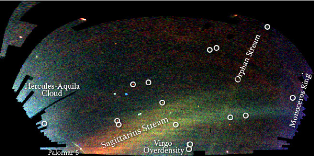
Figure 1.1: The “field of streams” of Belokurov et al. (2006). The observation of tens of millions of stars with SDSS, combined with appropriate cuts to the data, expose the dramatic merger-history substructure present in the Milky Way’s halo. The colours are for $r$ magnitude, which proxies for heliocentric distance in this image. The circles highlight clusters/galaxies newly discovered in this image. Credit: V. Belokurov and the Sloan Digital Sky Survey. Image source: sdss.org.

Fig. 1.1 shows one result of the effort: an on-sky map along the north Galactic pole, which was reported by Belokurov et al. (2006). This image shows the halo to be criss-crossed by extant tidal streams, and dotted with hitherto undetected low-mass halo-dwelling galaxies. Indeed, the observational evidence unearthed by the SDSS, and its follow-on extension programme (SEGUE, Yanny et al., 2009), revealed a dramatic number of tidal streams in the Milky Way halo, often with no obvious associated progenitor object (Odenkirchen et al., 2003; Majewski et al., 2003; Yanny et al., 2003; Belokurov et al., 2006, 2007; Grillmair, 2006a; Grillmair & Dionatos, 2006; Grillmair & Johnson, 2006; Grillmair, 2009; Newberg et al., 2009).

These streams are almost certainly the remnants of objects of extragalactic origin. Short of a major merger, it is hard to envisage a scattering event that could launch an existing Milky Way globular cluster onto a lower-energy orbit on which it cannot survive. Hence, it is likely that these streams originated either from former members of the cluster system of a larger cannibalized galaxy, which could not then survive on their new orbit around the Milky Way, or tiny galaxies whose streams are the fading echo of their cannibalization by the Milky Way in their own right.

The nature of the progenitors of these streams may be important for tracing the merger history of our Galaxy (Helmi, 2008). However, in this thesis, we will be concerned with the use of tidal streams as probes of the matter distribution of the Milky Way itself. As such, the details of their origin do not concern us greatly: we simply accept that at some point in their history, these objects have found their way onto orbits around our Galaxy, along which they experience tidal forces strong enough to promote their disintegration.

1.3 The use of tidal streams as probes of the potential

The possibility that the morphology of tidal tails from colliding galaxies could act as a probe of the potential has been recognized for almost as long as the physics of the tails themselves has been understood (Faber & Gallagher, 1979), although it is only much more recently (Dubinski et al., 1996) that simulation technology has been sufficient to make a serious attempt at constraining the potential with models of galaxies undergoing a major merger.

However, on account of the great disparity in mass between the Milky Way and its victims, the mergers observed are less violent than those seen between objects of similar mass. We should therefore be careful to distinguish the tidal streams resulting from the simple disintegration of clusters and small galaxies in the gravity field of a massive host—as is typically seen in the Milky Way—from those tidal tails, which result from major mergers. The stars of the former remain in low-energy orbits around the massive host, while the stars in the latter are unbound, or nearly so.

Furthermore, although the same fundamental physical principles underlie the creation of both species, the tidal streams that result from cannibalization of low-mass satellites, such as we see in the Milky Way halo, are almost certainly more useful than tails from major mergers in probing the potential of an individual galaxy. The reason is that major mergers must involve the catastrophic agglomeration of the dark matter haloes, wiping out all precursory substructure in favour of the newly virialized dark halo blob. Indeed, in the White & Rees (1978) model of galaxy formation it is the very occurrence of this dark-matter agglomeration which seals the fate of the merger. Hence, any probe of the dark matter distribution resulting from such a merger would be of comparatively little use in constraining the dark matter distribution of the precursor objects. Lastly, the unbound or marginally-bound tail stars from a major merger feel the gravity of their former hosts only weakly, which therefore has little effect on their motion, making them less sensitive probes overall.

The use of Milky Way streams as probes of the Galaxy potential stems from a recognition of the similarity between the trajectory of a stream, and the orbital trajectory of the progenitor object (McGlynn, 1990; Johnston et al., 1996). Observing the trajectory of an orbit places strong constraints on the gravitational force-field that gave rise to that trajectory, and hence also constrains the distribution of matter that generates that field (Binney, 2008). Indeed, it is precisely the knowledge of orbital trajectories in the Solar system that allows the mass of the Sun and the planets to be so well constrained. Similarly tight constraints can be placed on the mass of the Milky Way’s black hole, from the orbital trajectories of S-stars near the Galactic centre (Ghez et al., 2005).

In recognition of the diagnostic power of orbits, many recent papers have put some considerable effort into the attempt to locate the orbits delineated by tidal streams (Law et al., 2005; Fellhauer et al., 2007a, b; Odenkirchen et al., 2009; Willett et al., 2009; Koposov et al., 2010). Unfortunately, success in this endeavour, to date, has been somewhat limited. The traditional methods of finding orbits consistent with the data, namely, to search over a range of initial conditions from which one integrates the equations of motion, have resulted in fewer convincing fits to the data than might be expected (Eyre & Binney, 2009a).

Part of the problem is the enormous space of initial conditions that must be searched over. Even if one is lucky enough to stray upon an initial condition which reproduces an orbit roughly consistent with the data, it is not clear that a better match could not be found, with a different initial condition, and perhaps in a different potential. Ockham’s razor requires that we be able to convincingly falsify any theory of equal or lesser complexity to our own: to make a strong statement about the Galactic potential, we must be able to show that no other orbits in a given potential are compatible with the data.

“Geometrodynamical” methods—in the parlance of Jin & Lynden-Bell (2008)—are one answer to this difficulty. Such techniques utilize additional measurements of the stream, such as line-of-sight velocity measurements, to place additional constraints upon its trajectory (Jin & Lynden-Bell, 2007, 2008; Binney, 2008). These additional constraints substantially reduce the scope of the problem: solutions are now parameterized by the form of the potential and perhaps one other measurement. This substantial reduction in the space that parameterizes solutions makes an automated search over it feasible. Hence, the orbit consistent with a stream in a given potential can be isolated; or it can be shown that the data are incompatible with a given potential. This first half of the this thesis will advance the work of Jin & Lynden-Bell (2007) and Binney (2008) by specifying procedures to make such methods robust against errors in input data. We will also derive a new method, similar to the Binney (2008) procedure, but one that uses proper-motion measurement data as input instead of radial-velocity measurements.

Another issue that affects attempts to constrain the Galactic potential using streams is the degree to which the latter truly represent orbits. The belief that they do seems to originate in empiricist observations, made from the results of N-body simulations (e.g. McGlynn, 1990). Latterly, evidence has come to light, again from N-body simulations, that this belief may not be strictly true (Choi et al., 2007; Eyre & Binney, 2009b). Indeed, it turns out that the belief has no basis in classical mechanics, and quite the opposite is true: generally streams do not delineate orbits. In the second half of this thesis, we will demonstrate this from first principles. We will also examine techniques that attempt to ameliorate the use of such non-orbital stream data to constrain the Galactic potential.

1.4 Overview of this thesis

This thesis comprises several related studies in the dynamics of tidal streams around our Galaxy. The common thread that links these studies is the desire to exploit observations of tidal streams to place constraints upon the form of the Galactic potential.

The thesis is laid out in four substantive chapters according to the descriptions that follow. In addition to those, Chapter 6 reviews our findings in the context of astrophysics as a whole. We also provide some ancillary results to the calculations of Chapter 5 in Appendix A.

1.4.1 Chapter 2: Finding the orbits delineated by tidal streams

Binney (2008) and Jin & Lynden-Bell (2007) independently reported an algorithm for reconstructing full phase-space trajectories for tidal streams, given only the projection of a stream’s trajectory onto the plane of the sky, and measurements for the line-of-sight velocities everywhere along the stream. In this chapter, we demonstrate that the applicability of this algorithm is limited by errors in the input tracks from the following sources: likely statistical errors from observations, and systematic errors due to the fact that streams do not precisely delineate individual orbits.

We offer a procedure to overcome these difficulties by specifying a parameter space, which describes modifications to the baseline input in a way that is likely to correct for the above-mentioned errors while still remaining consistent with specified uncertainty in the baseline input. We then describe procedures to search over this parameter space, while applying the Binney (2008) algorithm to isolate those modifications that correspond to orbits. In this way, we are able to find orbits consistent with stream observations, without being hamstrung by errors in input data.

The ultimate goal of our work is to diagnose the Galactic potential. Binney (2008) showed that precise measurements of streams could place stunningly tight constraints on the potential. We illustrate the extent to which this is possible using realistic data.

1.4.2 Chapter 3: Fitting orbits to streams using proper motions

The major limitation on the work of Chapter 2 is the lack of line-of-sight velocity measurements to distant main-sequence stream stars. Although obtaining such measurements is within the capability of the technology of the day, it does require the commitment of 8-m class telescope time, which is unlikely to be forthcoming soon for more than a few streams.

In this chapter, we present a possible alternative: the probing of the potential using proper-motion measurements along streams. Following the same logical schema as is used in Binney (2008), we develop an algorithm to reconstruct the orbits of streams using such measurements. We find that it is equally efficacious to use proper-motion measurements of streams to reconstruct orbits and constrain the Galactic potential.

1.4.3 Chapter 4: Galactic parallax

Measuring distances in our Galaxy is critical to understanding its structure. However, line-of-sight distances can typically be measured with only relatively poor precision, and this lack of precision is manifest in the most basic of Galactic parameters, for instance, the distance to the Galactic centre (McMillan & Binney, 2010).

The gold standard of Galactic distance estimation is trigonometric parallax. However, its applicability is effectively limited to nearby stars. For more distant objects, alternative techniques such as photometric distance estimation must be used. Unfortunately, such non-geometric techniques necessarily rely on assumptions about stellar chemistry and composition that add complexity and uncertainty to measurements made using them.

The work of this chapter shows that by making use of the known trajectory of stream stars on the sky, and given accurate enough proper-motion measurements, it is possible to calculate trigonometric distances to stars in distant streams. This effect, which we call “Galactic parallax”, has a range some 40 times greater than that of conventional trigonometric parallax, given similarly accurate measurements of motion on the sky. We examine in detail the practicality and the limitations of distance estimation using the effect, and we demonstrate its utility by accurately computing the distance to the tidal stream GD-1 (Grillmair & Dionatos, 2006).

1.4.4 Chapter 5: The mechanics of streams

There has been some noise recently in the literature as to whether tidal streams can be taken to precisely delineate orbits (Choi et al., 2007; Eyre & Binney, 2009a, b). Standard techniques for constraining the potential by fitting orbits to streams rely upon the assumption that they can (e.g. Newberg et al., 2010). In this chapter, we demonstrate by use of analytical mechanics that streams, in general, do not delineate orbits. We further show that constraining the potential by assuming that streams make good proxies for orbits can lead to serious systematic error.

However, we also show that with relatively simple models of the phase-space distribution of disrupted clusters, it is possible to predict perfectly the trajectory of a stream, even when this differs significantly from the trajectory of a valid orbit. Thus, we conjecture it may be possible to repair the fitting algorithms, by having them utilize such stream trajectories instead.

Chapter 2 Finding the orbits delineated by tidal streams

2.1 Introduction

In this chapter, we first recount a procedure, independently described by Jin & Lynden-Bell (2007) and Binney (2008, herein B08), that permits the reconstruction of full phase-space information for an orbital trajectory, given only the assumption of the host Galaxy potential, and knowledge of both the track of the trajectory across the sky, and the rest-frame line-of-sight velocity down the track.

In B08 it was shown that, in addition to reconstructing phase-space information, by further examining which of the reconstructed trajectories (if any) constitute dynamical orbits, it is possible to utilize such tracks to diagnose the host potential. Given good enough input data, the precision with which both the trajectory can be reconstructed, and the potential diagnosed, was shown to be exquisite: distances and potential parameters are predicted to better than one per cent, which is far better than anything that has hitherto been possible with conventional techniques.

This advent of this procedure is particularly exciting in the context of Galactic astrophysics, since tidal streams from disrupted satellite galaxies have been held for some time to effectively delineate the orbit of their progenitor (Johnston et al., 1996; Odenkirchen et al., 2003). Thus, the detailed examination of the kinematics of these structures may well prove an important method for determining the nature of the Galactic potential.

The major limitations with the procedure as detailed in B08 are two-fold. Firstly, input data derived from observations will be subject to error, which limits the degree to which they can accurately represent an orbital track. Secondly, it has been noted (e.g. Choi et al., 2007) that tidal streams do not delineate individual orbits. This compromises a core requirement of the B08 procedure, since the input tracks now no longer represent dynamical orbits, and hence dynamics cannot be used to select the physical reconstructions from the unphysical ones.

The work of this chapter, much of which has been published in an article by Eyre & Binney (2009b), is devoted to examining these limitations, and exploring procedures by which they may be overcome.

The chapter is laid out as follows. §2.2 recounts some of the work of B08, upon which this chapter draws heavily, and demonstrates its limitations when applied to data for a simulated tidal stream. §2.3 briefly examines, with the aid of a simulated example, the constraints that observations of a stream’s track place on the orbits of the stream’s constituent stars. §2.4 describes procedures by which we identify those orbits (if any exist) that are consistent with such constraints. §2.5 tests the method, with the aid of a simulated example. §2.6 examines our ability to diagnose the host potential. In §2.7 we present our concluding remarks.

For the remainder of this chapter, the reference frame used is the inertial frame in which the Galactic centre is at rest; consequently line-of-sight velocities are obtained by subtracting the projection of the Sun’s motion from the measured heliocentric velocities. We assume complete knowledge of the velocity of the Sun with respect to the Galactic centre throughout most of this chapter.

Except where stated otherwise, orbits and reconstructions are calculated using the Galactic potential of Model II from Binney & Tremaine (2008, Table 2.3), which is a slightly modified version of a halo-dominated potential described by Dehnen & Binney (1998a). We take the distance to the Galactic centre to be $8\,{\rm kpc}$ and from Reid & Brunthaler (2004) (for $V$ and $W$) and Dehnen & Binney (1998b) we take the velocity of the Sun in the Galactic rest frame to be $(U,V,W)=(10.0,241.0,7.6)\,{\rm km}\,{\rm s}^{-1}$.

2.2 Reconstructing orbits from tracks on the sky

The following formulation for reconstructing complete phase-space information from a single point in space, an on-sky track, and the line-of-sight velocity measurements along that track, was discovered independently by Jin & Lynden-Bell (2007) and B08. Our work draws heavily on the latter formulation, so it is that formulation which we recount here.

Consider a tidal stream around the Galaxy, which we assume to delineate an orbit. Now let ${\bf r}$ be the position vector from the Sun to a star in this stream, let ${\bf v}$ be the rest-frame velocity of that star, and let $\Phi({\bf r})$ describe the potential of the Galaxy. At this point we assume the track to delineate an orbit perfectly, so its trajectory obeys the equations of motion

$$\ddot{{\bf r}}=-\nabla\Phi({\bf r})={\bf F}({\bf r}),$$ (2.1)

where ${\bf F}$ is the acceleration due to the gravity of the Galaxy. We define $v_{r}$ as the radial component of velocity,

$$v_{r}=\hat{{\bf r}}\cdot{\bf v}=\dot{r},$$ (2.2)

and we note that its derivative

$$\dot{v_{r}}=F_{r}+{\bf v}\cdot{{\rm d}\hat{{\bf r}}\over{\rm d}t},$$ (2.3)

where we have defined $F_{r}={\bf F}\cdot\hat{{\bf r}}$ as that component of the acceleration ${\bf F}$ along the line of sight. From the definition of ${\bf v}$ we have

$${\bf v}={{\rm d}(r\hat{{\bf r}})\over{\rm d}t}=v_{r}\hat{{\bf r}}+r{{\rm d}\hat{{\bf r}}\over{\rm d}t},$$ (2.4)

which rearranges to

$${{\rm d}\hat{{\bf r}}\over{\rm d}t}={\left({\bf v}-v_{r}\hat{{\bf r}}\right)\over r}.$$ (2.5)

Combining the above expression with equation (2.3), we find

$$\dot{v_{r}}=F_{r}+{\left(v^{2}-v_{r}^{2}\right)\over r}=F_{r}+{v_{t}^{2}\over r},$$ (2.6)

where ${\bf v}_{t}$ is the component of the star’s velocity in the plane of the sky. ${\bf v}_{t}$ must satisfy the relation

$$v_{t}^{2}=\left(r{{\rm d}\hat{{\bf r}}\over{\rm d}t}\right)^{2}=\ (r\dot{u})^{2}\equiv r^{2}\left(\dot{b}^{2}+\dot{l}^{2}\cos^{2}b\right),$$ (2.7)

where $(l,b)$ are the on-sky Galactic coordinates and where we now fix the meaning of the parameter $u$ to be the angular distance along the track. Combining equation (2.6) and equation (2.7), we obtain the non-linear ODE

$${{\rm d}v_{r}\over{\rm d}t}=F_{r}+r\left({{\rm d}u\over{\rm d}t}\right)^{2}.$$ (2.8)

We can rearrange this equation for ${\rm d}t/{\rm d}u$ as follows. Utilizing the chain rule and multiplying through by $({\rm d}t/{\rm d}u)^{2}$,

$${{\rm d}t\over{\rm d}u}{{\rm d}v_{r}\over{\rm d}u}=F_{r}\left({{\rm d}t\over{\rm d}u}\right)^{2}+r.$$ (2.9)

This equation is quadratic in ${\rm d}t/{\rm d}u$, and it can be solved for that quantity

$${{\rm d}t\over{\rm d}u}={1\over 2F_{r}}\left({{\rm d}v_{r}\over{\rm d}u}-\sqrt{\left({\rm d}v_{r}\over{\rm d}u\right)^{2}-4\,rF_{r}}\right),$$ (2.10)

where the choice of the negative root is made by requiring that ${\rm d}t/{\rm d}u$ is always positive. Equation (2.10) forms a system of coupled ODEs along with

$${{\rm d}r\over{\rm d}u}=v_{r}{{\rm d}t\over{\rm d}u},$$ (2.11)

which follows from the definition of $v_{r}$ and the chain rule.

Momentarily assume that the host potential $\Phi({\bf r})$ is known, and that the line-of-sight velocity $v_{r}(u)$ is known everywhere along an on-sky track $[l(u),b(u)]$. Given a single initial distance $r_{0}$ to some fiducial point on that track, equations (2.10) and (2.11) can be integrated. The resulting solution describes a trajectory for which full phase-space information is defined.

This result was reached independently by B08 and Jin & Lynden-Bell (2007), although the latter did not realize that only a subset of the solutions to equations (2.10) and (2.11) could be dynamical orbits. If one is to unlock the full diagnostic power of streams, it is important to isolate those solutions that are dynamical orbits. Further, if one can show that no solution of equations (2.10) and (2.11) with any initial distance $r_{0}$ is dynamical, then it follows that the assumed form for the host potential $\Phi({\bf r})$ must be wrong. B08 identified as dynamical those solutions with minimal rms orbital energy variation down the track, and for a given set of input data, isolated them all by means of a comprehensive search over $r_{0}$.

2.2.1 The problem with erroneous data

B08 showed that equations (2.10) and (2.11) can locate dynamical orbits with exquisite precision, if given perfect input data in the form of $[l(u),b(u)]$ and $v_{r}(u)$. The example in Fig. 2 of B08 showed this for an orbit in the Miyamoto-Nagai potential (Miyamoto & Nagai, 1975). However, B08 also showed that the ability of the technique to identify dynamical orbits quickly degrades when the input data are convolved with small random errors.

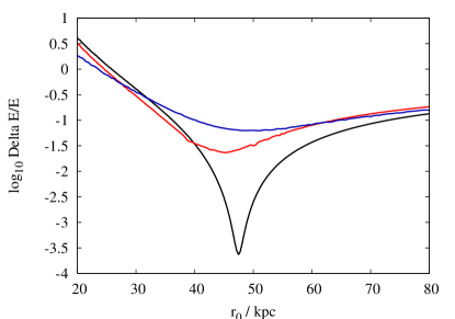
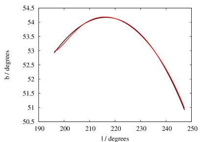
Figure 2.1: Left panel: normalized rms orbital energy, vs. initial distance to the stream $r_{0}$, for three input tracks. Right panel: on-sky plot of two tracks, used as the [l,b] input data for two of the curves in the left panel. The black curve in both panels is for the PD1 Test Orbit described in Table 2.1. The red curve in both panels is as the black curve, but with a small amount of random noise added to the input data. The blue curve is for a track derived from the simulated Orphan stream, shown in Fig. 2.2.

Fig. 2.1 demonstrates both these effects in the more realistic Model II potential used throughout this chapter. The right panel of Fig. 2.1 shows two on-sky tracks. The black track is the projection of a segment of the PD1 Test Orbit, described in Table 2.1. The red track is derived from the black track, but the input data $[l(u),b(u)]$ and $v_{r}(u)$ have been modified by the addition of random fluctuations, to $b(u)$ and $v_{r}(u)$, with the approximate amplitude of $3\,{\rm arcmin}$ and $0.35\,{\rm km}\,{\rm s}^{-1}$, respectively. The magnitude of these fluctuations is, respectively, smaller than the on-sky width of the narrowest known stream, and smaller than the velocity-measuring precision of an 8m-class spectrograph-equipped telescope when observing distant stream stars. Thus, such fluctuations are plausible estimates for likely errors introduced by the observational process. We note that the resulting red track is only marginally distinguishable from the black track, even at the augmented scale of the right panel of Fig. 2.1.

Using each of the tracks in the right panel, trajectories were reconstructed using equations (2.10) and (2.11) for a range of initial distances $r_{0}$. Along each such reconstructed trajectory, the normalized rms orbital energy variation

$${\Delta E\over E}\equiv\sqrt{{\langle E^{2}\rangle\over{\langle E\rangle}^{2}}-1},$$ (2.12)

was computed, where $E_{i}=v_{i}^{2}/2+\Phi({\bf r}_{i})$ at a point ${\bf r}_{i}$ along the track. The numerical scheme used in the solution of equations (2.10) and (2.11) was identical to that of B08, save for a minor upgrade to the endpoints of the splines, detailed in §2.4 below.

The left panel of Fig. 2.1 shows $\Delta E/E$ versus initial distance $r_{0}$, when each of the black and red tracks is used as input. In the case of the perfect input of the black track, the correct initial distance $r_{0}\simeq 47\,{\rm kpc}$ is identified with little scope for error, since $\Delta E/E$ reaches a deep and sharp minimum at that point. However, the effect of the random fluctuations in the input data on the ability to identify dynamical orbits has been very damaging. The depth of the minimum has decreased by two orders of magnitude, and the minimum has changed location to $r_{0}\simeq 45\,{\rm kpc}$. Although perhaps the extreme distances of $r_{0}\sim 20\,{\rm kpc}$ and $r_{0}\sim 80\,{\rm kpc}$ could still be ruled out, there is now only a marginal basis on which to select a distance at $r_{0}\simeq 45\,{\rm kpc}$ over another distance, since a different random fluctuation could put the easily-moved minimum elsewhere. Most disappointingly, all power to identify dynamical orbits from amongst the reconstructed trajectories has been lost, since the best trajectory only conserves energy to one part in 40, which would wash out most of the exquisite detail shown in Fig. 3 of B08, which was key to the ability of that work to diagnose the potential.

Table 2.1: Parameters of highlighted orbits from this chapter. The coordinate system used is right-handed with $\hat{x}$ pointing away from the Galactic centre and $\hat{y}$ opposite the sense of Galactic rotation.

	position (x,y,z)$\rm/kpc$	velocity (x,y,z)$/\!\,{\rm km}\,{\rm s}^{-1}$
N-body Orphan	$(28.1,-10.0,34.0)$	$(-89.2,-37.1,-76.2)$
PD1 Test Orbit	$(35.5,7.80,37.8)$	$(-7.97,56.3,47.8)$

We therefore conclude that the B08 procedure does not cope well with likely observational error.

2.2.2 The problem with real streams

The previous section, and the work of B08 that it recaps, are predicated on the assumption that streams precisely delineate orbits. Recent studies involving N-body simulations of such streams (e.g. Dehnen et al., 2004; Choi et al., 2007) have made it clear that they do not. Chapter 5 of this thesis investigates the mechanics of tidal stream formation in some detail, and concludes with the ability to predict the tracks of tidal streams with high precision. However, to motivate the work of this chapter, which was reported by Eyre & Binney (2009b) before the work of Chapter 5 was undertaken, we content ourselves with the examination of an N-body simulation of a stream superficially similar to the Orphan stream of Belokurov et al. (2007).

 

 

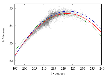
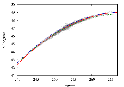
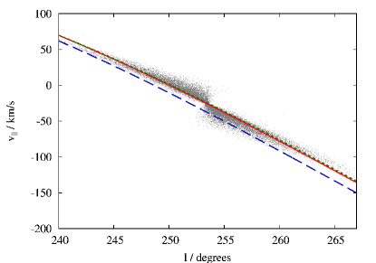
Figure 2.2: Full (red) lines: the orbit of a progenitor of an Orphan-like stream. Broken (green/blue) lines: orbits of a star now seen at either end of the tidal tail. Points: particles tidally stripped from an N-body model of the Orphan-like progenitor. Upper panels: distributions on the sky; lower panels: line-of-sight velocities. The N-body model had 60,000 particles set up as a King model with $W=2$, $r_{0}=13.66\,{\rm pc}$ and $M_{0}=9381M_{\odot}$, on the orbit detailed in Table 2.1, and evolved for $9.43\,{\rm Gyr}$. The particles were advanced in time by the fvfps tree code of Londrillo et al. (2003).

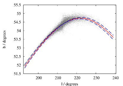
Figure 2.3: The dots are the projection of the simulated Orphan stream particles onto the sky. The red curve is a smooth polynomial fit to a set of points selected by eye to lie down the stream track. An input track $b(l)$ was defined by sampling 30 points from this curve, which was then used as input for the blue line in Fig. 2.1, and as baseline input for the data sets PD2–PD7. The blue dashed lines are the upper and lower bounds for PD2–PD7, as set by the penalty function $p_{\rm pos}$ (equation 2.23), and therefore represent the bow-tie region for these data sets.

The full red curves in Fig. 2.2 show projections of an orbit (described in Table 2.1) outwardly similar to that underlying the Orphan Stream, from two viewing locations: the position of the Sun and a position $120^{\circ}$ further round the Solar circle. Also shown in each projection are the locations of particles tidally stripped from a self-gravitating N-body model of a cluster launched on to that orbit. Clearly the particles provide a useful guide to the orbit of the cluster, but they do not precisely delineate it. Moreover, the relationship of the projected orbit to the stream depends on viewing angle. The line-of-sight velocities of the particles have a similar relationship to the orbit’s line-of-sight velocity. Hence even with perfectly error-free observations, the track of a stream will not coincide with the progenitor orbit.

What would be the result of attempting to utilize the track of this stream in the procedure of B08? A set of points $\{l,b\}$ and $\{l,v_{r}\}$ was selected from the simulation output, by eye, to lie down the middle of the stream. These sets were each fitted with a low-order polynomial to ensure smoothness, and these polynomials were sampled at 30 points to produce a set of input data, $b(l)$ and $v_{r}(l)$. The polynomial curves can be seen, along with the simulation data from which they derive, in Figs. 2.3 and 2.4.

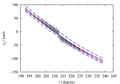
Figure 2.4: The dots are line-of-sight velocities for the particles of the simulated Orphan stream. The red curve is a smooth polynomial fit to a set of points selected by eye to lie down the stream track. An input track $v_{r}(l)$ was defined by sampling 30 points from this curve, and was used as input for the blue line in Fig. 2.1, and as baseline input for the data sets PD2–PD4. Also shown, as dashed blue lines, are the bow-tie regions for PD2 (narrow) and PD4 (wide). The bounds of these regions are enforced by the penalty function $p_{\rm vel}$ (equation 2.25).

The input data were used to solve the reconstruction equations (2.10) and (2.11) for a range of initial distances $r_{0}$. The blue curve in the left panel of Fig. 2.1 shows $\Delta E/E$ for the reconstructed trajectories. Unlike with the black curve, the minimum in the blue curve is very shallow, with energy conservation being half an order of magnitude worse than that of the erroneous input data, and $2{1\over 2}$ orders of magnitude worse than that of the perfect input data. It is not possible to make any statement about the true distance to the stream, or the validity of the potential, from the blue curve in Fig. 2.1.

Quite apart then from uncertainties in the observational data, the failure of tidal streams to properly delineate orbits has been shown to limit the diagnostic power of the B08 procedure. Therefore, in order to fully exploit the dynamical potential of streams, we have to understand how to infer the location of an underlying orbit from measurements of the stream.

For the moment we assume that any errors in measured quantities are negligible, which in practice means that they are small compared to the intrinsic width of the stream. This condition will certainly be satisfied by the on-sky coordinates. It will not always be satisfied by the velocity data, so we address the issue of velocity errors below.

2.3 Specifying stream tracks

With what precision could the track of an orbit be specified from the positions of the particles in Fig. 2.2? First we need to be clear that any orbit will do. Generally it will be convenient to use the orbit that passes through some point that lies near the centre of the observed stream, both on the sky and in line-of-sight velocity. In some circumstances this orbit will closely approximate the orbit of the centroid of the stream’s progenitor, but there is no requirement for it to do so. Since a single fiducial point on the orbit can be chosen at will, this point is associated with vanishing uncertainty. As one moves away from this point, either up or down the stream, it becomes more uncertain where the chosen orbit lies, and the size of the uncertainties must increase. Hence the region of $(l,b,v_{r})$ space to which the orbit is confined by the observations is widest at its extremities and shrinks to a point at its centre. We call this the “bow-tie region.”

In the top panels of Fig. 2.2 the leading and trailing streams are not offset for much of the span, so our first guess may be that the orbit of the centroid runs right down the centre of the stream. In the lower panels the stream has a kink at the progenitor and our best guess is that the orbit through the point where the two halves of the tail touch runs near the lower edge of the left-hand half and near the upper edge of the right-hand half. In every case the uncertainty in the location of the orbit grows from zero at the centre to roughly half the width of the stream at its ends. Quantitatively, the largest uncertainty is then $0.15^{\circ}$ for the top-left panel, $\sim 0.25^{\circ}$ for the top-right panel, and $\sim 5\,{\rm km}\,{\rm s}^{-1}$ in the bottom panels.

2.4 Identifying dynamical orbits

B08 showed that given an orbit’s projection onto the sky $[l(u),b(u)]$ and the corresponding line-of-sight velocities $v_{r}(u)$, the remaining phase space coordinates can be recovered by solving the differential equations (2.10) and (2.11).

If the input data used to solve those equations are not derived from an orbit in the same force field as is used to derive $F_{r}$, the reconstructed phase-space coordinates will not satisfy the equations of motion. B08 observed that violation of the equations of motion might cause the reconstructed solution to violate energy conservation, and therefore used rms energy variation down the track as a diagnostic for the quality of a solution. However, energy conservation is necessary but not sufficient to qualify a track as being an orbit. Here we construct a diagnostic quantity from residual errors in the equations of motion themselves, since orbits are defined to be solutions of these equations.

We first derive the equations of motion. In the Galactic rest-frame, the canonically conjugate momenta to the Galactic coordinates $(r,b,l)$ are

$$p_{r} =\dot{r},$$

$$p_{b} =r^{2}\dot{b},$$ (2.13)

$$p_{l} =r^{2}\cos^{2}b\,\dot{l},$$

and the Hamiltonian is

$${\rm H}=\frac{1}{2}p_{r}^{2}+\frac{1}{2}\frac{p_{b}^{2}}{r^{2}}+\frac{1}{2}\frac{p_{l}^{2}}{r^{2}\cos^{2}b}+\Phi(r,b,l).$$ (2.14)

The equations of motion are therefore

$$\dot{p_{r}} =\ddot{r}=\frac{p_{b}^{2}}{r^{3}}+\frac{p_{l}^{2}}{r^{3}\cos^{2}b}-\frac{\partial\Phi}{\partial r},$$

$$\dot{p_{b}} =\ddot{b}r^{2}+2\dot{b}\dot{r}r=-\frac{p_{l}^{2}}{r^{2}}\frac{\sin b}{\cos^{3}b}-\frac{\partial\Phi}{\partial b},$$ (2.15)

$$\dot{p_{l}} =r^{2}\ddot{l}\cos^{2}b-2r^{2}\dot{l}\dot{b}\,\sin b\,\cos b+2r\dot{r}\dot{l}\cos^{2}b=-\frac{\partial\Phi}{\partial l}.$$

As in B08, when solving equations (2.10) and (2.11) we make extensive use of cubic-spline fits to the data. In the examples presented in B08 natural splines were used in order to avoid specifying the gradient of the data at its end points. Significantly improved numerical accuracy can be achieved by taking the trouble to specify these gradients explicitly. Given input data, we estimate the quantity ${{\rm d}l}/{{\rm d}b}$ at the end points by fitting a quadratic curve through the first three and last three points. ${{\rm d}l}/{{\rm d}b}$ is then computed at the location of the middle point of each set, and the very first and very last points are considered ‘used’ and thrown away. This quantity is then used in the geometric relation

$$\frac{{\rm d}u}{{\rm d}b}=\pm\sqrt{1+\cos^{2}b\left(\frac{{\rm d}l}{{\rm d}b}\right)^{2}},$$ (2.16)

to compute ${{\rm d}b}/{{\rm d}u}$ at the ends of the track. The sign ambiguity is resolved by inspection of the directionality of the input data. We then use the geometric relation

$$\frac{{\rm d}l}{{\rm d}u}=\pm\sec b\sqrt{1-\left(\frac{{\rm d}b}{{\rm d}u}\right)^{2}},$$ (2.17)

to obtain ${{\rm d}l}/{{\rm d}u}$ at the ends of the track, where the sign ambiguity is resolved in the same way. We are now able to fit cubic splines through the input tracks, with the slopes at the ends of the $l(u)$ and $b(u)$ tracks given as above, but at this stage the track of $v_{r}(u)$ is fitted with a natural spline. The reconstruction equations (2.10) and (2.11) are now solved for $t(u)$, which is then fitted with a cubic spline, with the slopes at the ends given explicitly by equations (2.10) and (2.11) themselves.

We can now compute $l(t)$ and $b(t)$ and fit splines to them, with the slopes at the ends computed from ${{\rm d}l}/{{\rm d}u}$ and ${{\rm d}b}/{{\rm d}u}$ by the chain rule. The momenta (2.4) are now calculated explicitly, using the derivatives of the splines for $l(t)$ and $b(t)$ in place of $\dot{l}$ and $\dot{b}$. The slopes at the endpoints, ${{\rm d}v_{r}}/{{\rm d}u}$, can now be calculated from equation (2.4) and ${{\rm d}t}/{{\rm d}u}$; the $v_{r}(u)$ spline is refitted using these boundary conditions, the reconstruction repeated, and the momenta recalculated.

To compute a diagnostic quantity, the left- and right-hand sides of the equations of motion (2.4) are now evaluated explicitly. For each equation of motion we define a residual

$$R(t)=\dot{p}_{\rm lhs}(t)-\dot{p}_{\rm rhs}(t).$$ (2.18)

These residuals are used to compute, for each equation of motion, the diagnostic quantity

$$D=\log_{10}\left(\frac{\int_{t_{1}}^{t_{2}}{\rm d}t\,R(t)^{2}}{\int_{t_{1}}^{t_{2}}{\rm d}t\,\dot{p}_{\rm lhs}^{2}}\right),$$ (2.19)

where the residuals have been normalized by the mean-square acceleration and the times $t_{1}$ and $t_{2}$ correspond to the fifth and fifth-from-last input data points: numerical artefacts from the end regions, $0<t<t_{1}$ and $t_{2}<t<t_{\rm max}$, tend to dominate the integrated quantity and are not easily reduced by modifying the input; these regions are therefore excluded. The largest of the three values for $D$ is used as the diagnostic quantity for that particular input.

2.4.1 Parameterizing tracks

Our strategy for identifying a stream’s underlying orbit is to compute the diagnostic $D$ (equation 2.19) for a large number of candidate tracks, and to find which candidates yield values of $D$ consistent with their being dynamical orbits.

We start by specifying a baseline track across the sky $[l_{\rm b}(u^{\prime}),b_{\rm b}(u^{\prime})]$, where $u^{\prime}$ is a parameter that increases monotonically down the track from $-1$ to $1$. Similarly, we specify associated baseline line-of-sight velocities $v_{r\rm b}(u^{\prime})$. The baseline track is required to come closer to every data point than the given uncertainty at that point.

All candidate tracks should be smooth because orbits are. We satisfy this condition by expressing the difference between the baseline track and a candidate track as a low-order polynomial in $u^{\prime}$. For streams that cover a wide range of longitudes, the parameterization of candidate tracks is achieved by slightly changing the values of $b$ and $v_{r}$ associated with a given value of $l$ from the values specified by the baseline functions. That is we write

$$b(u^{\prime}) =b_{\rm b}(u^{\prime})+\sum_{n=0}^{N}b_{n}T_{n}(u^{\prime}),$$

$$v_{r}(u^{\prime}) =v_{r\rm b}(u^{\prime})+\sum_{n=0}^{N}a_{n}T_{n}(u^{\prime}),$$ (2.20)

where $T_{n}$ is the $n^{\rm{th}}$-order Chebyshev polynomial of the first kind and $a_{n}$ and $b_{n}$ are free parameters. These $2N$ parameters are coordinates for the space of tracks that we have to search for orbits. When a stream does not stray far from the Galactic plane, candidate tracks are best parameterized by adjusting the baseline values of $b$ and $v_{r}$ at given longitude. In all examples in this chapter, the series in equations (2.4.1) are truncated after $N=10$. A larger number of terms allows the correction function to produce tracks that represent orbits better, while using insufficient terms will fail to afford sufficient flexibility for the search procedure to find any orbits at all. However, using more terms makes the search procedure computationally more expensive, because the volume of the parameter space in which the search takes place grows exponentially with the number of terms, and locating solutions in this enlarged space requires commensurately more effort. The number of terms used is therefore a compromise between computational expense and the ultimate efficacy of the algorithm.

The space of tracks is defined by the $a_{n}$ and $b_{n}$ and one extra parameter, the distance to the stream, $r_{0}$, at the starting point $u=0$ for the integration of equations (2.10) and (2.11).

We shall henceforth denote a point in the ($2N+1$)-dimensional space of parameters by $\chi$. Each $\chi$ is associated with a complete specification of all six phase-space coordinates for every point on the candidate orbit: $l$, $b$ and $v_{r}$ follow from the parameterization and the remaining coordinates are obtained by solution of the differential equations (2.10) and (2.11). Consequently, each $\chi$ corresponds to a value of $D$ (equation 2.19) that quantifies the extent to which the phase-space coordinates deviate from a dynamical orbit in the given potential.

2.4.2 Searching parameter space

Dynamical orbits are found by minimizing the sum

$$D^{\prime}(\chi)=D(\chi)+p(\chi),$$ (2.21)

where $p(\chi)$ is the sum of the penalty functions:

$$p(\chi)=\sum_{i}p_{i,\rm pos}+\sum_{i}p_{i,\rm vel}+p_{s},$$ (2.22)

where

$$p_{i,\rm pos}=\begin{cases}\Delta_{i,\rm pos}&\text{if $\Delta_{i,\rm pos}>1$},\\ 0&\text{otherwise},\end{cases}$$ (2.23)

with

$$\Delta_{i,\rm pos}={\left|b(l_{i})-b_{\rm b}(l_{i})\right|\over\delta b(l_{i})}.$$ (2.24)

Here $\delta b_{i}$ is the width in $b$ of the bow-tie region at $l_{i}$. Similarly

$$p_{i,\rm vel}(l)=\begin{cases}\Delta_{i,\rm vel}&\text{if $\Delta_{i,\rm vel}>1$},\\ 0&\text{otherwise},\end{cases}$$ (2.25)

with

$$\Delta_{i,\rm vel}={\left|v_{r}(l_{i})-v_{r\rm b}(l_{i})\right|\over\delta v_{r}(l_{i})}.$$ (2.26)

Prior information about the distance to the stream is used by specifying the penalty function $p_{\rm s}$ to be

$$p_{\rm s}=\left\{\begin{array}[]{ll}\beta\left|r_{0}-r_{0\rm b}\right|/\delta r&\quad\mbox{if $\left|r_{0}-r_{0\rm b}\right|>\delta r$},\\ 0&\quad\mbox{otherwise},\end{array}\right.$$ (2.27)

where $\delta r$ is the half-width of the allowed range in the distance $r_{0}$ to the starting point of the integrations and $r_{0\rm b}$ is the baseline value of $r_{0}$. These definitions are such that $p(\chi)=0$ so long as the track lies within the region that is expected to contain the orbit, and rises to unity, or in the case of $p_{\rm r}$ to $\beta$, on the boundary and then increases continuously as the orbit leaves the expected region.

In practical cases the prior uncertainty in distance is large, and the obvious way to search for orbits is to set $\delta r$ to the large value that reflects this uncertainty and then set the algorithm described below to work. It will find candidate orbits for certain distances. However, we shall see below that it is more instructive to search the range of possible distances by setting $\delta r$ to a small value such as $0.5\,{\rm kpc}$ and searching for orbits at each of a grid of values of $r_{0\rm b}$. In this way we not only find possible orbits, but we show that no acceptable orbits exist outside a certain range of distances. In this procedure the logic underlying $\delta r$ is very different from that underlying $\delta b$ and $\delta v_{r}$.

Since $p(\chi)$ is added to the logarithm of the rms errors in the equations of motion and since it increases by of order unity at the edge of the bow-tie region, the algorithm effectively confines its search to the bow-tie region, where $p=0$. Thus at this stage we do not discriminate against orbits that graze the edge of the bow-tie region in favour of ones that run along its centre. Our focus at this stage is on determining for which distances dynamical orbits can be constructed that are compatible with the data. Once this has been established, distances that lie outside some range can be excluded from further consideration.

The space of candidate tracks $\chi$ is 21-dimensional, so an exhaustive search for minima of $D^{\prime}$ (equation 2.21) is impractical. Furthermore, the landscape specified by $D^{\prime}$ is complex. Some of this complexity is physical; the space should contain continua of related orbits, and ideally $D^{\prime}\to-\infty$ at orbits. Hence deep trenches should criss-cross the space. Superimposed on this physical complexity is a level of numerical noise arising from algorithmic limitations in the computation of $D^{\prime}(\chi)$. The limitations include the use of finite step sizes in the solution of equations (2.10) and (2.11) and the subsequent evaluation of $D^{\prime}(\chi)$, the inability of a finite series of Chebyshev polynomials to precisely describe a true orbital track, as well as the difficulty in representing this series with a collection of sparse input points interpolated with splines. Reconstructed tracks are therefore never perfect orbital trajectories, even when the method is initially presented with error-free input data, and this is manifest as a non-zero minimum residual for each equation of motion. In practice, this minimum residual sets a lower limit on the returned values of $D^{\prime}(\chi)$, which we refer to as the “numerical-noise floor”.

On account of the complexity of the landscape that $D^{\prime}$ defines, “greedy” optimization methods, which typically follow the path of steepest descent, are not effective in locating minima. The task effectively becomes one of global minimization, which is a well studied problem in optimization.

We have used the variant of the Metropolis “simulated annealing” algorithm described in Press et al. (2002), which uses a modified form of the downhill simplex algorithm. In the standard simplex algorithm, the mean of the values of the objective function over the vertices decreases every time the simplex deforms. In the Press et al. algorithm the simplex has a non-vanishing probability of deforming to a configuration in which this mean is higher than before. Consequently, the simplex has a chance of crawling uphill out of a local minimum. The probability that the simplex crawls uphill is controlled by a “temperature” variable $T$: when $T$ is large, uphill moves are likely, and they become vanishingly rare as $T\to 0$. During annealing the value of $T$ is gradually lowered from an initially high value towards zero.

One vertex of the initial simplex is some point $\chi_{\rm guess}$, and the remaining $2N+1$ vertices are obtained by incrementing each coordinate of $\chi_{\rm guess}$ in turn by a small amount. For the coefficients of the Chebyshev polynomial $T_{0}$ this increment is approximately the size of the allowed half widths, $\delta r,\delta v$ and $\delta b$. Increments for coordinates representing coefficients of higher-order polynomials $T_{n}$ are scaled as $1/n$. The overall size of these increments is therefore set by the size of the region within which we believe the global minimum to lie. It is important to note that in each generation of a simplex, the increments should independently have equal chance of being added to or subtracted from the values of $\chi_{\rm guess}$ so that no part of the parameter space is unfairly undersampled. The algorithm makes tens of thousands of deformations of the simplex while the temperature $T$ is linearly reduced to zero. This entire process is repeated some tens of times, after which we have a sample of local minima that are all obtained from $\chi_{\rm guess}$.

We now update $\chi_{\rm guess}$ to the location of the lowest of the minima just found and initiate a new search. The entire process is repeated until the value of the diagnostic function $D^{\prime}(\chi)$ hits a floor. When this floor lies higher than the numerical-noise floor, the attempt to find an orbit that is consistent with the assumed inputs has been a failure and we infer that no such orbit exists. When the floor coincides with the numerical-noise floor, we conclude that the corresponding $\chi$ specifies an orbit that is compatible with the inputs. An approximate value for the numerical-noise floor for a given problem may be obtained as follows: given input that perfectly delineates an orbit in the potential in use, the value of $D^{\prime}$ returned at the correct distance is approximately the numerical-noise floor. Conclusive proof that a candidate track with a particular value of $D^{\prime}$ is an orbit can be obtained by integrating the equations of motion from the position and velocity of any point on the track and ensuring that the time integration essentially recovers the track.

On account of the stochastic nature of the algorithm, an attempt to find a solution at a particular distance occasionally sticks at a higher value of $D^{\prime}$ than the underlying problem allows. This condition is identified by scatter in the values of $D^{\prime}$ reached on successive attempts and by inconsistency of these values with the values of $D^{\prime}$ achieved for nearby distances—we see from Fig. 2.5 that the function underlying the minima is smooth. When the magnitude of this scatter is significant, one can only confidently declare an attempt to find an orbit a failure if the $D^{\prime}$ achieved is consistently higher than the noise floor by more than the scatter; since the diagnostic measure $D^{\prime}$ quantifies the extent to which a candidate track satisfies the equations of motion, by definition, tracks with higher $D^{\prime}$ than the noise floor plus scatter cannot represent orbits.

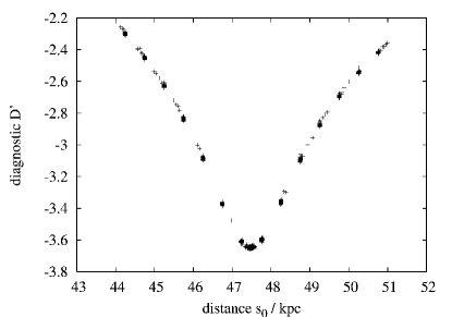
Figure 2.5: Values of the diagnostic function $D^{\prime}$ for candidate orbits reconstructed from the pseudo-data set PD1. Each group of crosses is associated with one of 15 ranges within which the starting distance $r_{0}$ was constrained to lie. For each such range the candidate orbit was reconstructed from 280 trial tracks, and each track yields a cross. In this figure the crosses are largely superimposed because the uncertainties are small and there is little scope for tweaking the track. This figure can be compared directly with the black curve of Fig. 2.1, the structure of which is clearly reflected in these results.

When the observational constraints are weak, we expect several orbits to be compatible with them. In particular, we will be able to find acceptable orbits for a range of initial distances $r_{0}$. It is therefore important, for any given input, to run the algorithm starting from many different values of $r_{0\rm b}$ with $\delta r$ set to prevent the algorithm straying far from the specified $r_{0\rm b}$. In this way, the full range of allowable distances can be mapped out, and dynamical orbits found for each distance in that range. In the case of significant scatter about the noise floor, the range of distances at which valid orbits are found is the range within which solutions yield values of $D^{\prime}$ smaller than the noise floor plus scatter. Similar degeneracies in the parameters controlling the astrometry and line-of-sight velocities are less of a concern because if we have orbits that differ in these observables, we simply concentrate on the orbit that lies closest to the baseline track.

2.5 Testing the method

To test this method, we used the N-body approximation to the Orphan Stream shown in Fig. 2.2 as our raw data. The baseline input data $b_{b}(l)$ and $v_{rb}(l)$ were chosen to be the same 30-point samples of the smooth red curves from Figs. 2.3 and 2.4 as was used in §2.2.2 to test the B08 procedure. To the baseline data we attached uncertainties $\delta b$ and $\delta v_{r}$, which through the penalty functions $p_{\rm pos}$ and $p_{\rm vel}$ (equations 2.23 and 2.25) constrain the tracks that the Metropolis algorithm can try. Details of the resulting pseudo-data sets are given below, and are summarised in Table 2.2.

Table 2.2: Configurations of pseudo-data sets used to test the method.

	$\delta v_{r,{\rm max}}/\!\,{\rm km}\,{\rm s}^{-1}$	$\delta v_{r,{\rm min}}/\!\,{\rm km}\,{\rm s}^{-1}$	offset $v_{r}/\!\,{\rm km}\,{\rm s}^{-1}$
PD1	$2\times 10^{-3}$	$2\times 10^{-3}$	0
PD2	4	0	0
PD3	6	2	0
PD4	10	10	0
PD5	6	2	2
PD6	15	10.5	10
PD7	4	0	0

In one case, PD1, the above baseline input data were replaced by those of a perfect orbit and $\delta b$ and $\delta v_{r}$ set very narrow ($6\,$arcsec and $2\times 10^{-3}\,{\rm km}\,{\rm s}^{-1}$) in order to validate the reconstruction algorithm.

The uncertainty $\delta b(l)$ takes the same value for all the remaining pseudo-data sets because we assume that the astrometry is sufficiently precise for the uncertainty in position to be dominated by the offset of the stream from an orbit. In all cases, $\delta b$ has a maximum value of $0.15^{\circ}$ at the ends of the stream, falling linearly to zero at the position of the progenitor, consistent with the orbit of the progenitor seen in Fig. 2.2. Fig. 2.3 shows this input alongside the N-body data from which it was derived.

For the pseudo-data sets PD2 and PD3, $\delta v_{r}$ is set to a maximum at the ends of the stream, and falls linearly to a minimum of zero and $2\,{\rm km}\,{\rm s}^{-1}$ respectively, at the position of the progenitor. These examples represent a case (PD2) in which the uncertainty in radial velocity is dominated by stream width, and a case (PD3) in which there is a significant contribution from measurement error at a level that is easily obtainable with a spectrograph. The pseudo-data set PD4 represents the case in which the uncertainty in $v_{r}$ is dominated by measurement errors: $\delta v_{r}$ is held fixed at $10\,{\rm km}\,{\rm s}^{-1}$, which is typical for the measurement errors in the line-of-sight velocities of SDSS stars in distant streams. Fig. 2.4 shows the input for these data sets.

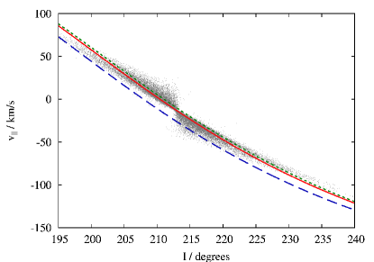
Figure 2.6: The broken lines show input tracks $v_{r}(l)$, as used for data sets PD5 (dotted green) and PD6 (dashed blue). The unmodified input of PD2 (full red curve) is shown for comparison. The dots are line-of-sight velocities for the particles of the simulated Orphan stream, from which the input was derived.

For the pseudo-data sets PD5 and PD6, we added to the baseline data systematic offsets in $v_{r}(l)$ to mimic systematic errors in radial velocity. $\delta v_{r}$ varies between a maximum and a minimum as in PD2 and PD3, with the values set to encompass the (assumed known) systematic bias. Fig. 2.6 shows the input for these data sets.

The pseudo-data set PD7 is identical to that of PD2, except that the number of raw $(l,v_{r})$ points was reduced to just three: one at either end of the N-body stream, and one at the location of the progenitor. A quadratic curve was perfectly fitted through these three points, and sampled at 30 locations to produce the baseline $v_{r}(l)$ input. $\delta v_{r}$ is set to the same maximum value as PD2 at the outermost points; $\delta v_{r}$ is set to zero at the centre point. Only these three points are allowed to contribute to the penalty function (2.25) in this pseudo-data set.

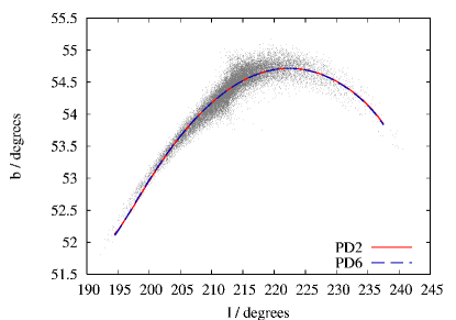
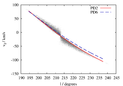
Figure 2.7: Left panel: projections onto the sky of two candidate orbits and the N-body data from which the input was derived. The full curves show the candidate orbit at $46\,{\rm kpc}$ from PD2, and the dashed curves show the candidate orbit at $43\,{\rm kpc}$ from PD6. Right panel: line-of-sight velocity down the track for the same candidate orbits. The penalty function (2.22) forces the sky projection and radial velocity curves of candidate orbits to be consistent with the data; the equivalent plots for all other tracks are very similar to these examples.

In all of the examples, the penalty function (2.22) acts to constrain the candidate tracks to be consistent with the data. The contribution of the penalty function to $D^{\prime}$ is therefore zero in all examples. All candidate tracks are guaranteed to be consistent with the data, even if they do not represent dynamical orbits. Fig. 2.7 provides example plots of $(l,b)$ and $(l,v_{r})$ for candidate tracks from PD2 and PD6 along with the raw N-body data from which the baseline data are derived. Equivalent plots for all candidate tracks are similar to these.

For PD1, PD2 and PD3, and each of 15 values of the baseline distance $r_{0\rm b}$, 280 optimization attempts were made, each involving Metropolis annealing for 24,000 simplex deformations, from an initial temperature of 0.5 dex. The starting distances were constrained by the penalty function $p_{s}$ (equation 2.27) with $\beta=10^{6}$ and $\delta r=0.5\,{\rm kpc}$, so the Metropolis algorithm could only explore a narrow band in $r_{0}$. After 40 optimization attempts from a given starting point $\chi_{\rm guess}$, the starting point was updated to the end point of the most successful of these optimizations, and annealing recommenced from a high temperature. In total 6 of these updates were performed. With these parameters, a search at a single distance completes in 12 CPU-hours on 3GHz Xeon-class Intel hardware. PD4, PD5 and PD6 follow almost the same schema, except that 48,000 simplex deformations were made for each of 60 attempts at the same $\chi$, which was updated 6 times. A single distance in the latter case took 36 CPU-hours to search: the computational load scales linearly with the number of deformations considered.

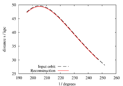
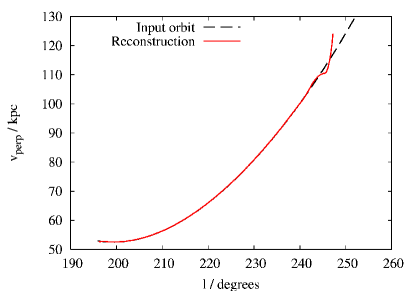
Figure 2.8: The left panel shows heliocentric distance, $r$, versus galactic longitude, $l$, for the best reconstruction from Fig. 2.5 and for the true orbit from which the input was generated. The two curves are close to overlying. The right panel shows tangential velocity, $v_{t}$, for the best reconstruction and for the true orbit: the departure of the reconstruction from the orbit near the endpoints is symptomatic of the problems near the endpoints that necessitate their excision from the diagnostic.

Fig. 2.5 shows the results obtained with PD1, which has very small error bars. The diagnostic function $D^{\prime}$ has a smooth minimum that pinpoints the distance $r_{0}=47.4\,{\rm kpc}$ to the starting point with an uncertainty of $\sim 0.2\,{\rm kpc}$. The Metropolis optimization can significantly reduce $D^{\prime}$ by tweaking the input track only when $r_{0}$ is close to the truth. The depth of the minimum indicates the numerical-noise floor for this particular problem, and no significant scatter is seen between successive runs. We do expect the noise floor to be slightly different for PD2–PD6 because both the underlying orbits and the input are somewhat different. Fig. 2.8 shows that the reconstructed solution at the minimum overlies the input orbit almost exactly. We conclude that when the error bars are as small as in PD1, only one orbit is consistent with the data.

The left panels of Fig. 2.9 show the results obtained with PD2, PD3 and PD4. For PD2 and PD3, which have small to moderate error bars, the Metropolis algorithm reduces $D^{\prime}$ to the noise floor only for $r_{0}$ in the range $(44,46)\,{\rm kpc}$. The scatter between runs is small, $\sigma_{D^{\prime}}\sim 0.1$. The left panels of Figs. 2.10 and 2.11 show the reconstructed distances and tangential velocities associated with the best two solutions found at $44$ and $46\,{\rm kpc}$. With PD2, these reconstructions provide a distance estimate to the stream that is, at worst, $2\,{\rm kpc}$ in error, and a $v_{t}$ estimate that is at worst $5\,{\rm km}\,{\rm s}^{-1}$ in error. With PD3, the reconstruction is, at worst, $3\,{\rm kpc}$ and $10\,{\rm km}\,{\rm s}^{-1}$ in error. For many sections of the orbits, the errors are less than stated. Thus the method can identify orbits consistent with the stream, and reject those that are inconsistent with it.

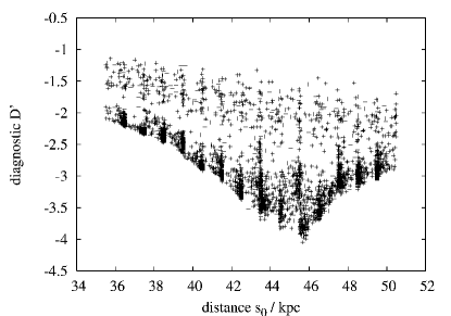
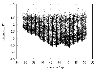
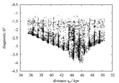
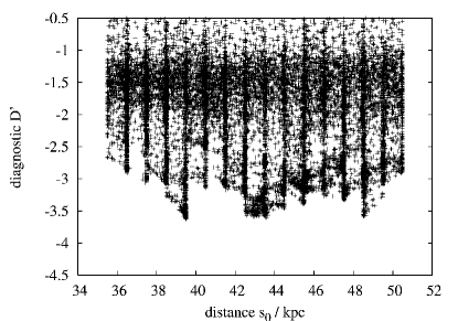
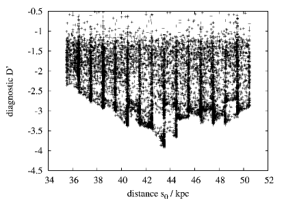
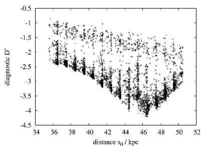
Figure 2.9: The same as Fig. 2.5 but for input data sets: PD2 (upper-left), PD3 (middle-left), PD4 (lower-left), PD5 (upper-right), PD6 (middle-right) and PD7 (lower-right). In PD2 and PD3, the noise floor $D^{\prime}\sim-4$ is reached only for starting distances in the range $44-46\,{\rm kpc}$. In PD4 we find an isolated good solution at $43\,{\rm kpc}$, but in contrast to what happens with data sets PD2 and PD3, as we change distance the value of $D^{\prime}$ oscillates around $\sim-3.25$ for most of the range, rather than varying smoothly. This behaviour arises because the volume of parameter space that has to be searched is large on account of the largeness of the velocity errors. Such an extensive volume of parameter space cannot be exhaustively searched with the allocated computational resource. Only orbits with $r_{0}<40\,{\rm kpc}$ could be excluded with confidence. In PD5 and PD6, the noise floor $D\sim-3.5$ is now approached over a wider range in $r_{0}$: $42-47\,{\rm kpc}$ in PD5 with some confidence, and $38-48\,{\rm kpc}$ in PD6 with little confidence. As the errors increase, the search becomes a more arduous task, and patchy performance of this task is reflected in the rough bottoms to the graphs. In PD7, the results are very similar to those of PD2 and PD3, with a noise floor $D^{\prime}\sim-4$ and solutions acceptable only in the range $44-46\,{\rm kpc}$.

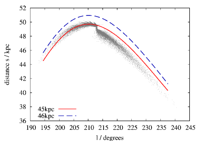
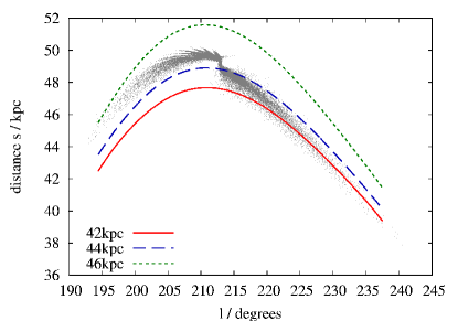
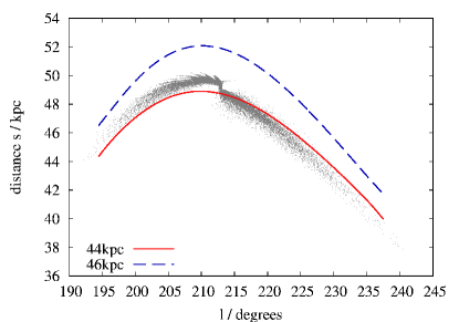
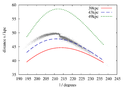
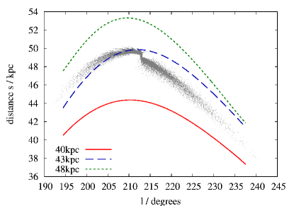
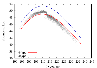
Figure 2.10: Heliocentric distance for selected reconstructed orbits from the data sets: PD2 (upper-left), PD3 (middle-left), PD4 (lower-left), PD5 (upper-right), PD6 (middle-right) and PD7 (lower-right). The tracks selected are those with lowest $D^{\prime}$ at distances for which $D^{\prime}$ approaches the noise floor in Fig. 2.9.

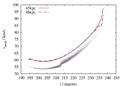
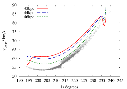
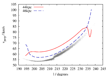
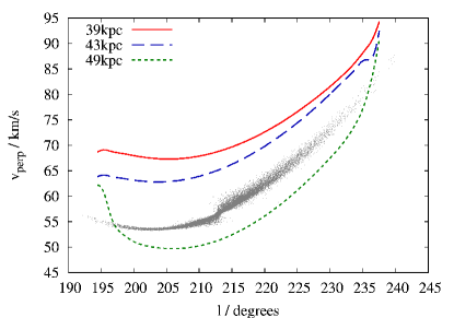
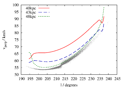
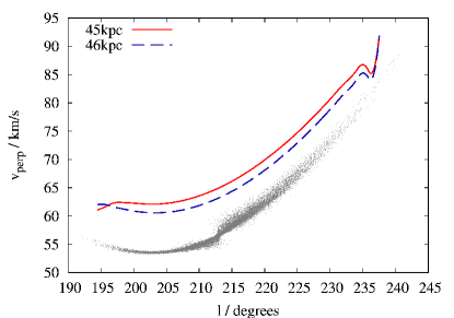
Figure 2.11: Tangential velocities for selected reconstructed orbits from the data sets: PD2 (upper-left), PD3 (middle-left), PD4 (lower-left), PD5 (upper-right), PD6 (middle-right) and PD7 (lower-right). The tracks selected are the same as in Fig. 2.10.

For PD4, which has large error bars comparable to those for velocity data from the SDSS, scatter between repeat runs is much larger, $\sigma_{D^{\prime}}\sim 0.5$. Only distances $r_{0}<40\,{\rm kpc}$ can be confidently excluded, although a high-quality solution near $r_{0}\sim 43\,{\rm kpc}$ provides a reconstruction in error by at most $2\,{\rm kpc}$ in distance and $5\,{\rm km}\,{\rm s}^{-1}$ in $v_{t}$. Figs. 2.10 and 2.11 show us that ignoring this high-quality solution would give reconstructed quantities in error by up to $5\,{\rm kpc}$ in distance and $12\,{\rm km}\,{\rm s}^{-1}$ in $v_{t}$. Increasing the errors associated with the input clearly permits less satisfactory solutions to be returned, and also decreases the ability of the search procedure to find true orbits at particular distances, should they exist, by increasing the volume of parameter space it has to search. The former complaint is a physical statement about the limitations of the input data. The latter complaint is an algorithmic one, which may be remedied by providing the search with more computational cycles, or improving its efficiency.

The upper-right and middle-right panels of Fig. 2.9 shows the results obtained from input sets PD5 and PD6, in which offsets were applied to the input velocities. The reconstructed distances and tangential velocities for interesting tracks are shown in the upper-right and middle-right panels of Figs. 2.10 and 2.11. For PD5, the scatter between runs is $\sigma_{D^{\prime}}\sim 0.5$, and the distance to the stream $r_{0}$ can be said to lie in the range $42-47\,{\rm kpc}$ with some confidence. Fig. 2.10 shows that the stream does indeed lie in this range, so the algorithm has successfully corrected the small offset. The error in reconstructed distance and $v_{t}$ would be $3\,{\rm kpc}$ and $8\,{\rm km}\,{\rm s}^{-1}$ at worst.

PD6 demonstrates the limits of the method. On account of the large scatter in $D^{\prime}$, $\sigma_{D^{\prime}}\sim 1$, we cannot identify the correct distance from the middle-right panel of Fig. 2.9. We expect the distance range for permitted orbits to be wide with this input, because the velocity error bars are large. PD5 and PD6 illustrate another problem of using large error bars: the search becomes harder because the parameter space to be searched is much larger. Consequently the plots of the results for PD5 and PD6 have rough bottoms, where the algorithm has failed to reach consistent minima for searches at adjacent distances. This can be remedied by re-running the search with more deformations and more iterations, and may be addressed in future upgrades to the search procedure.

PD7 demonstrates that the accuracy of the method is not necessarily significantly degraded when the number of velocity data points is substantially lower than the number of positional data points, as might be expected from a stream for which the only available radial velocities are those of giant stars. The results for PD7 are shown in the bottom-right panel of Fig. 2.9 and are directly comparable to those of PD2 and PD3 (the upper-left and middle-left panels). In particular, the range of allowed distances, $44-46\,{\rm kpc}$, is the same and the reconstructed orbits show comparable accuracy (cf. the upper-left and bottom-right panels of Figs. 2.10 and 2.11).

2.6 The effect of changing the potential

B08 demonstrated the ability of orbit reconstruction to diagnose the Galactic potential with astonishing precision when the track of an orbit on the sky is precisely known. Here we investigate the ability of orbit reconstruction to identify the correct potential when the track has to be inferred from realistic stream data.

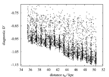
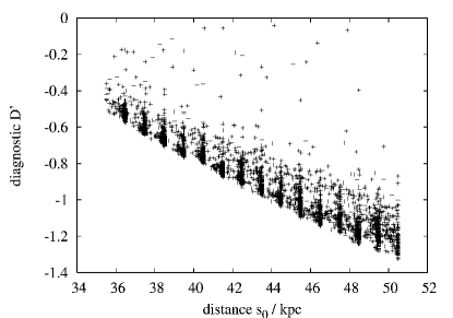
Figure 2.12: As Fig. 2.5, except the reconstruction (using PD2) takes place in a Kepler potential (left panel), and (right panel) a potential with $\Phi(r)\propto r$. In both cases, the potential parameters are set to generate approximately the same passage time along the stream as in Model II. Comparing with Fig. 2.9 shows the values of $D^{\prime}$ achieved are very poor, demonstrating that no orbits can be found in these potentials, which can therefore be excluded.

We use as our input the PD2 data set from §2.5. The left panel of Fig. 2.12 shows the results of asking the algorithm to find orbits in a Kepler potential with mass $M=4.18\times 10^{11}M_{\odot}$, which produces roughly the same passage time along the stream as does Model II. The right panel shows the results obtained using a potential of the form $\Phi(r)=rf_{r}$, which gives a rotation curve of the form $v_{c}(r)=\sqrt{rf_{r}}$ with $f_{r}=6.86\times 10^{2}(\,{\rm km}\,{\rm s}^{-1})^{2}/\,{\rm kpc}$, again chosen to produce the same passage time along the stream as does Model II. These two potentials represent, respectively, relatively extreme falling and rising rotation curve models. We do not offer them as realistic candidates for the Galactic potential, but we intend to demonstrate that model potentials with approximately correct radial force, but incorrect shape, can be excluded using this method.

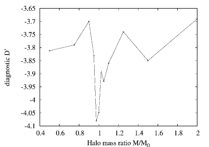
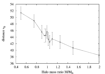
Figure 2.13: The left panel shows the minimum value of the diagnostic for attempted reconstruction of the PD2 input, versus the halo mass ratio of the Dehnen-Binney potential in which the reconstruction has been attempted. $M_{0}$ here is the value of the halo mass in the Model II potential. The right panel shows the characteristic distance, $r_{0}$, of the best solution, versus halo mass ratio. The error bars represent the approximate uncertainty in the recovered result.

The distance range considered in both cases spans approximately $\pm 15$ percent of the true distance, which is the uncertainty one might expect in distances obtained by photometry. Since all values of $D^{\prime}$ are several orders of magnitude larger than the values one obtains with the correct potential, it is clear that no orbits can be found at the distances considered, and both potentials can be excluded.

Fig. 2.13 shows the results of reconstructing an orbit from the PD2 data set in a potential that differs from the Model II potential used to define the tidal stream only in that the halo mass has been varied by the specified ratio. This high-quality data set yields a sharp minimum in $D^{\prime}$ as a function of $r_{0}$ (cf. the upper-left panel of Fig. 2.9) and the left panel of Fig. 2.13 shows this minimum value of $D^{\prime}$ as a function of assumed halo mass. The minimum of $D^{\prime}$ lies at $D^{\prime}<-4$ when the mass used lies within $\sim 5$ percent of the true value and $D^{\prime}>-3.85$ otherwise. Hence, with high-quality data it is possible to constrain with remarkable precision the parameters of a model potential that is otherwise of the correct shape.

Uncertainty estimates for potential parameters deduced in this way present some difficulty. Any parameters for which the minimum value of $D^{\prime}$ returned is greater than the noise floor are inconsistent with the data, and should be rejected. The uncertainty associated with each parameter is therefore that range over which solutions can be found that are consistent with the noise floor. Ambiguity arises, however, because the value of the noise floor itself must be estimated from the data, and is therefore uncertain. Furthermore, it is not clear with what probability an otherwise consistent set of parameters would return a value of $D^{\prime}$ higher than the noise floor, on purely stochastic grounds. In practice, potential parameters can only be confidently excluded if the scatter in returned value of $D^{\prime}$ is substantially smaller that the difference between $D^{\prime}$ and the noise floor, and yet the precise level of this confidence remains difficult to formally quantify.

The right panel of Fig. 2.13 shows the value of $r_{0}$ at which $D^{\prime}$ attains its minimum, as a function of assumed halo mass. We see that this value decreases systematically as the halo mass increases. Insight into this behaviour can be obtained by considering the discretized equation of angular-momentum conservation

$$\Delta(r\,v_{t})=-r\Delta t\,\nabla_{t}\Phi=-r{\Delta v_{r}\over F_{r}}\,\nabla_{t}\Phi,$$ (2.28)

where $-\nabla_{t}\Phi=(\hat{{\bf r}}\cdot\nabla\Phi\,\hat{{\bf r}}-\nabla\Phi)$ is the component of the force in the plane of the sky, and where $\Delta$ implies the change in a quantity between successive data points. By expanding the left side to first order in small quantities we can obtain an expression for $\Delta v_{t}$. Summing the changes in $v_{t}$ along the track we have

$$v_{t}(\hbox{end})-v_{t}(\hbox{start})=-\sum\left(\nabla_{t}\Phi\,{\Delta v_{r}\over F_{r}}+v_{t}{\Delta r\over r}\right).$$ (2.29)

An independent equation for $v_{t}$ is

$$v_{t}=r{\Delta u\over\Delta t}=rF_{r}{\Delta u\over\Delta v_{r}},$$ (2.30)

where we have used the radial component of Newton’s second law. Equations (2.29) and (2.30) yield independent estimates of $v_{t}(\hbox{end})-v_{t}(\hbox{start})$. The right side of equation (2.29) yields an estimate that is independent of the scaling of $\Phi$ but systematically decreases with increasing $r$, while the right side of equation (2.30) yields an estimate that is proportional to the scaling of $\Phi$, but is almost independent of $r$, since $F_{r}\propto 1/r$. When the machine is asked to reconstruct the orbit with $F_{r}$ taken too small, it can change the right side of equation (2.29) to match the new value of the right side of equation (2.30) by increasing $r$. In this way, the discrepancies between the left sides of equations (2.29) and (2.30), which contribute substantially to the diagnostic $D^{\prime}$, can be largely eliminated by increasing $r$ as $\Phi$ is scaled down.

In principle this variation in reconstructed distance with the scaling of the potential could be combined with photometric distances to constrain the potential. Unfortunately, Fig. 2.13 shows that in the particular geometry under consideration, even a $10$ percent distance error would produce a $\sim 50$ percent error in the estimate of the halo mass. Further work is required to discover what effect the geometry of a particular stream has on its sensitivity to the potential. Also of interest is whether simultaneously using multiple streams, or streams with multiple wraps (such as the Sagittarius Dwarf stream), can provide yet tighter constraints on the potential—B08 indicated that much could be gained from this approach, but more work is needed to extend the present schema to handle multiple independent segments of streams.

2.7 Conclusions

B08 demonstrated the tremendous diagnostic power that is available if one knows the track of an orbit on the sky and the associated line-of-sight velocities. Tidal streams are made up of stars that are on similar orbits. In particular, they roughly delineate the underlying orbit, but they do not do so exactly. We have presented a technique for identifying an underlying orbit and thus predicting the dynamical quantities that have not been observed, such as the distances to the stream and the proper motions of its particles.

A complete summary of our findings of this chapter is presented below. Following the summary is a discussion of the limitations of the work, accompanied by suggestions on how to overcome those limitations. Chapter 6 further reviews our findings in the context of contemporary astrophysics.

2.7.1 Summary

The technique presented involves defining a space of tracks on the sky and sequences of line-of-sight velocities that are consistent with the observational data, given the observational errors and the extent to which streams deviate from orbits. The equations of B08 are used to determine a candidate orbit for each track, and then the extent to which the candidate satisfies the equations of motion is quantified. This represents an enhancement over B08, in which only violations of energy conservation along a candidate were quantified. The resulting diagnostic quantity is used to search for tracks that could be projections of orbits in the Galactic potential. In practice the search is conducted for several possible distances to a fiducial point on the stream. If constraints on this distance are available from photometry, the computational effort of the search can be reduced by narrowing the range of distances for which searches need to be conducted. Our a priori assumptions are knowledge of the Galaxy’s gravitational potential, and the Sun’s velocity with respect to the Galactic centre.

The technique is moderately computationally expensive, in practice taking several CPU-core hours to process a given set of input for a single fiducial distance and potential combination. This computational expense arises from the large number of dimensions of the parameter space that the technique must search over: the parameter space must be sufficiently large to afford the technique the flexibility to derive a dynamical track from the input data, but the computational time that must be devoted to the search to ensure that the parameter space is appropriately explored grows exponentially with the dimensionality of the parameter space. The number of dimensions selected in practice is a compromise between these considerations. In mitigation, the search does lend itself to simple parallelization, and with a few dozen CPU-cores it is feasible to fully analyze a stream in a given potential in less than a day.

Our tests revolve around an N-body model of the Orphan Stream (Belokurov et al., 2007) on the assumption that it formed by the disruption of a globular cluster. We show that for this stream, which is $\sim 40^{\circ}$ long and $0.3^{\circ}$ wide at its ends, distances to and tangential velocities of points on the stream can be recovered to within $\sim 2\,{\rm kpc}$ and $\sim 5\,{\rm km}\,{\rm s}^{-1}$, respectively, if line-of-sight velocities accurate to $\sim 1\,{\rm km}\,{\rm s}^{-1}$ are measured. As the errors in the measured radial velocities increase, the space of tracks that must be considered grows bigger and the search for acceptable orbits becomes more laborious. Moreover, the range of distances for which acceptable orbits can be found broadens. However, even with errors in radial velocities as large as $\pm 10\,{\rm km}\,{\rm s}^{-1}$, the uncertainties in the recovered distances are no greater than $\sim 10$ percent and the recovered tangential velocities are accurate to better than $\sim 20$ percent. Zero-point errors in the input velocities that are reflected in appropriately wide error bars broaden the range of acceptable orbits but do not skew the results.

We have shown that the method maintains its accuracy even when very few radial velocity points are used to define the input, as might be necessary when radial velocities can only be measured for giant stars. In our tests, comparable results were obtained from pseudo-data based on only three velocity measurements and from pseudo-data based on fifteen velocity measurements. Indeed, the results obtained with three accurate velocity measurements were significantly superior to those obtained with fifteen lower-quality measurements. Naturally, exactly how many points are required to provide well-determined input will depend on the shape of the radial velocity curve along the stream in question.

We expect the accuracy of reconstructions to depend on the geometry of the problem in hand. In particular, we expect streams at apocentre, where families of orbits are compressed both on the sky and in radial velocity, to yield poorer results than streams away from apocentre. Unfortunately, streams are most likely to be discovered at apocentre because both trajectory compression and low proper motions around apocentre lead to a high density of stars at apocentre. We expect streams that are relatively narrow to produce more accurate results, because the permitted deviation of the orbit from the stream is then low. We also expect to have more difficulty reconstructing orbits from streams that contain a visible progenitor, since the potential of the progenitor will cause orbits in the progenitor’s vicinity to differ materially from orbits in the Galaxy’s underlying potential.

B08 suggested that it should be possible, if sufficiently accurate input is provided, to constrain the Galactic potential, since the wrong potential will not admit an acceptable orbit. We have tested this possibility for input with realistic errors. We find that two potentials of significantly different shape, the Kepler potential and $\Phi(r)\propto r$, are clearly excluded. We have also tested for changes in scaling of an otherwise correctly-shaped potential, by varying the mass of the assumed dark halo around the value used to make the pseudo-data. In this case, we find the correct potential is identified, with the diagnostic quantity generally worsening as the halo mass moves away from its correct value by more than $\sim 5$ percent. We further find a consistent relationship between the reported stream distance and the halo mass with which the reconstruction takes place. Although the reported distance is only weakly dependent upon halo mass, this does open the possibility of using alternative distance measurements, such as photometric distances, in conjunction with these techniques to constrain the Galactic potential.

Further work is necessary to determine a full scheme to recover parameters of the potential from stream data. Also in question is the extent to which simultaneous reconstruction of multiple streams, and reconstruction of streams with multiple wraps around the Galaxy, might provide stronger constraints on the Galactic potential than the short section of a single wrap that we have considered. It may also prove possible to refine the other main assumption of our scheme, the location and velocity of the Sun.

2.7.2 Discussion

It is interesting to compare our method of finding orbits of progenitors with the traditional N-body method. Firstly, our method explores each orbit at a tiny fraction of the computational expense of N-body modelling, so it is feasible to automate the search of orbit space. Moreover, the search lends itself to easy parallelization. Finally, whereas only a successful attempt to model a stream with N body simulation yields an interesting conclusion, our method can show that no orbit is consistent with a given range of distances. This latter facility is particularly powerful, because by guaranteeing that no consistent orbit can be found, it is possible to test our assumed form for the Galactic potential.

The most serious limitation on the applicability of this work is the lack of high precision radial velocity measurements for streams. At the time of preparation of the Eyre & Binney (2009b) work on which this chapter draws, the radial velocity data available for a long, cold stream were scant: perhaps the best available were the two data points for the Orphan stream of Belokurov et al. (2007), which were held by the authors to be “suggestive rather than conclusive”.

Since then, the situation has improved somewhat. Newberg et al. (2010) have recently reported radial velocity measurements for 7 fields along the Orphan stream, deriving from recently released SDSS/SEGUE spectra of giant stars. The measurements have associated uncertainties of $\sim\!10\,{\rm km}\,{\rm s}^{-1}$. The GD-1 (Grillmair & Dionatos, 2006) and Anticentre streams (Grillmair, 2006b) are closer to the Sun than is the Orphan stream, and therefore make easier targets for observations. Grillmair et al. (2008) obtained radial velocity data for two fields along the Anticentre stream (Grillmair, 2006b), with an accuracy of $\sim\!7\,{\rm km}\,{\rm s}^{-1}$. Koposov et al. (2010) combined SDSS/SEGUE spectra and purposely-obtained spectra of 24 main sequence and turn-off stars, and although they do not do so, their results could perhaps be organized into four or five fields with uncertainties of $\sim 4\,{\rm km}\,{\rm s}^{-1}$ in each.

The procedures in this chapter could be immediately applied to all these streams. However, our experiments with pseudo-data indicate that the strongest constraints on the potential are to be had from $\sim\!1\,{\rm km}\,{\rm s}^{-1}$ precision data, rather than $\sim\!10\,{\rm km}\,{\rm s}^{-1}$ precision data. Except for perhaps the Koposov et al. (2010) observations of GD-1, the available radial velocity data do not meet this requirement.

Part of the problem stems from the need to use only the brightest stars in order to obtain useful spectra on the small-aperture telescopes that have so far been used for this work. The density of such stars associated with tidal streams is low, which are by their nature dynamically old structures, and are often barely distinguishable from the field stars even in the main sequence. The few giant stars that are observed are insufficient in number to beat down the observational random errors to the required level. The problem is made worse by the difficultly in convincingly identifying giant stars with streams, with the small statistics involved leading to the possibility of a single contaminant star ruining an entire field.

Obtaining radial velocity measurements of streams with the required accuracy will necessitate the observation of main-sequence stars. Observations of main-sequence stars in distant streams such as the Orphan stream would require the use of $8\,$m-class equipment for what is superficially unglamourous work. However, the results of this chapter indicate that the scientific rewards of such an undertaking would be far-reaching.

Chapter 3 Fitting orbits to streams using proper motions

3.1 Introduction

The previous chapter has demonstrated the remarkable diagnostic power that orbit reconstruction from observed stream tracks can have, when coupled with radial velocity measurements down those streams.

However, it was proffered that perhaps the most serious problem afflicting such work is the difficulty in obtaining precise radial velocity measurements of stars in such streams, and particularly of the faint main-sequence stars that constitute the bulk of the prospective data.

One possible workaround to reconstruct phase-space tracks using measured proper motions rather than radial velocities. This is attractive because, although it is much harder to make an impromptu proper-motion measurement than it is to take a spectrum, it is possible to measure very many of the former simultaneously, down to the faint apparent magnitudes of main-sequence stars in distant streams.

This kind of work is already possible to some extent with the combined SDSS-USNO catalogue of Munn et al. (2004), as demonstrated by Koposov et al. (2010), who obtain comparatively high precision proper-motion measurements for the GD-1 stream (Grillmair & Dionatos, 2006) from lower-precision Munn et al. raw data, on account of the hundreds of main-sequence stars they are able to identify. By comparison, their spectroscopically-obtained radial velocity data number only in the dozens, with even this frugal number making GD-1 the best observed object in its class. Furthermore, with the advent of advanced astrometric projects such as the Pan-STARRS survey (Kaiser et al., 2002, currently commissioning), and its follow-on project LSST (Tyson, 2002), the future availability of large amounts of high-quality proper-motion data for main-sequence stars is assured. We note that Pan-STARRS proper motions will be obtained for stars seven visual magnitudes fainter than those to be observed by Gaia (Perryman et al., 2001).

In the work of this chapter, much of which has been published in an article by Eyre & Binney (2009a), we derive a set of equations that can reconstruct full-phase space information from an on-sky track, if proper-motion magnitudes are measured everywhere along that track. The application of this technique is logically identical to the reconstruction of trajectories using radial-velocity data (Jin & Lynden-Bell, 2007; Binney, 2008; Chapter 2). We will demonstrate numerically that the reconstructed tracks can be tested for dynamicity, just as were those in Chapter 2. We further illustrate that the ability to use reconstructed tracks as probes of the Galactic potential is retained when using proper-motion data.

The remainder of this chapter is arranged as follows. §3.2 derives a set of reconstruction equations that use proper motions to generate candidate orbit trajectories. §3.3 demonstrates the efficacy of the reconstruction equations with a numerical test. §3.4 discusses our findings and sums up.

3.2 Reconstructing orbits with proper motions

As in Chapter 2, we derive a reconstruction algorithm on the basis that a stream precisely delineates an orbit. The probable effects of this incorrect assumption will be noted when applications of the work are discussed.

Consider two inertial frames of reference: one in which the Galactic centre is at rest (the grf), and another in which the Sun is instantaneously at rest (the hrf). In the grf, let ${\bf x}_{0}$ be the position vector of the Sun, ${\bf x}$ the location of a star in the stream and let ${\bf r}$ be the vector from the Sun to the star. By definition

$${\bf r}=r\hat{{\bf r}}={\bf x}-{\bf x}_{0},$$ (3.1)

where $\hat{{\bf r}}$ is the direction from the Sun to the star. Now let ${\bf x}^{\prime}$ be the vector obtained by transforming ${\bf x}$ from the grf frame to the hrf. Again, by definition

$${\bf r}^{\prime}=r^{\prime}\hat{{\bf r}}^{\prime}={\bf x}^{\prime}-{\bf x}^{\prime}_{0}.$$ (3.2)

Consider the measurement of $\hat{{\bf r}}$ and $\hat{{\bf r}}^{\prime}$, each made by one two observers, both at the location of the Sun, but each in his respective frame. Instantaneously the frames must coincide, so ${\bf r}={\bf r}^{\prime}$ at that given moment. However, the instantaneous derivatives ${\rm d}\hat{{\bf r}}/{\rm d}t$ and ${\rm d}\hat{{\bf r}}^{\prime}/{\rm d}t$ will not be equal. The former derivative is tangent to the stream, and is the proper motion that would be made by an observer stationary with respect to the Galactic centre. The latter derivative is the terrestrial observable proper motion of the star, and includes a component perpendicular to the stream, due to the reflex motion of the Sun. Diagrams illustrating these configurations are shown in Fig. 3.1.

 

Figure 3.1: Diagrams illustrating the velocities of the Sun and of a stream of stars, as seen from (left) the Galactic rest-frame, and (right) the heliocentric rest-frame. Black arrows represent the velocities of objects. The components of velocity along the line-of-sight (blue arrows), and in the plane of the sky (red arrows), are shown for a star in the stream at position ${\bf r}$. A section of the plane of the sky at the radius $r$ is shown as a dotted red circle, while the dashed red line shows the tangent to that circle at the position ${\bf r}$. Note that, even while the stream stars have been taken to follow one another in the grf, in the hrf the velocities of the stream stars do not point along the stream.

Now let $u$ be the on-sky angle along the stream from some fiducial point. We may write

$$\frac{{\rm d}\hat{{\bf r}}^{\prime}}{{\rm d}t}=\mu\hat{{\bf t}};\qquad\frac{{\rm d}\hat{{\bf r}}}{{\rm d}t}=\dot{u}\hat{{\bf p}},$$ (3.3)

where $\mu$ and $\hat{{\bf t}}$ are the magnitude and direction of the measured proper motion, while $\dot{u}$ and $\hat{{\bf p}}$ are the on-sky magnitude and direction of the star’s motion along the stream. Space velocities measured in the grf differ from those measured in the hrf by the velocity of the Sun, that is

$${{\rm d}{\bf r}^{\prime}\over{\rm d}t}={{\rm d}{\bf r}\over{\rm d}t}-{\bf v}_{0},$$ (3.4)

where ${\bf v}_{0}$ is the grf velocity of the Sun. Differentiating equations (3.1) and (3.2), and combining the results with equation (3.3) and equation (3.4), we obtain

$${{\rm d}{\bf r}\over{\rm d}t} =\dot{r}\hat{{\bf r}}+r\mu\hat{{\bf t}}$$

$$={{\rm d}{\bf r}^{\prime}\over{\rm d}t}-{\bf v}_{0}=\dot{r}^{\prime}\hat{{\bf r}}^{\prime}+r^{\prime}\dot{u}{\bf p}-{\bf v}_{0}=\dot{r}^{\prime}\hat{{\bf r}}+r\dot{u}{\bf p}-{\bf v}_{0},$$ (3.5)

where in the last step we have made use of the instantaneous equality ${\bf r}={\bf r}^{\prime}$. We note that ${\rm d}r^{\prime}/{\rm d}t=\dot{r}^{\prime}$ is the spectroscopically measured heliocentric velocity, and that ${\rm d}r/{\rm d}t=\dot{r}=v_{r}$ is the projection along the line of sight of the star’s velocity with respect to the Galactic centre. Equating the components in the plane of the sky, we have

$$r\mu\hat{{\bf t}}=r\dot{u}\hat{{\bf p}}-({\bf v}_{0}-\hat{{\bf r}}\cdot{\bf v}_{0}\,\hat{{\bf r}})=r\dot{u}\hat{{\bf p}}-{\bf v}_{s},$$ (3.6)

where ${\bf v}_{s}$ is the component of the Sun’s velocity perpendicular to the line of sight. This equation has just two unknowns, $\dot{u}$ and $r$, and we can in principle solve for both through

$$\dot{u}\hat{{\bf p}}=\mu\hat{{\bf t}}+\frac{{\bf v}_{s}}{r}.$$ (3.7)

Specifically, since both $\hat{{\bf t}}$ and $\hat{{\bf p}}$ can in principle be deduced from the observations and ${\bf v}_{s}$ may be presumed known, we could determine $r$ such that the right side is parallel to $\hat{{\bf p}}$, and then read off $\dot{u}$ from the magnitude of the right side. Startlingly, this permits the distance to the stream to be recovered from the observables with no additional assumptions. This method embodies the idea of Galactic parallax, and is examined further in Chapter 4. For now, we will consider that case where the uncertainty in the direction $\hat{{\bf t}}$ is significant, prohibiting the use of the Galactic parallax procedure. We proceed to eliminate $\hat{{\bf t}}$ by squaring up

$$(\dot{u})^{2}-2\frac{{\bf v}_{s}\cdot\hat{{\bf p}}}{r}\dot{u}+\frac{\left|{\bf v}_{s}\right|^{2}}{r^{2}}-\mu^{2}=0.$$ (3.8)

The roots of this quadratic equation in $(r\dot{u})$ are given by,

$$r\dot{u}={\bf v}_{s}\cdot\hat{{\bf p}}\pm\sqrt{({\bf v}_{s}\cdot\hat{{\bf p}})^{2}+(r\mu)^{2}-\left|{\bf v}_{s}\right|^{2}}.$$ (3.9)

The sign ambiguity is resolved as follows. Using this expression to eliminate $\dot{u}$ from equation (3.7), we find

$$\mu\,\hat{{\bf t}}\cdot\hat{{\bf p}}=\pm\sqrt{({\bf v}_{s}\cdot\hat{{\bf p}})^{2}-\left|{\bf v}_{s}\right|^{2}+(r\mu)^{2}}.$$ (3.10)

Since $\mu$ is inherently positive, we see that the sign of the radical in equation (3.9) must be chosen to agree with the sign of $\hat{{\bf t}}\cdot\hat{{\bf p}}$. Even though the directions of individual proper motions may be uncertain, it should be possible to decide whether they are on average opposed to the direction of travel along the stream. This ambiguity resolved, equation (3.9) now makes $\dot{u}$ into a function of both $r$ and quantities that can be determined from the observations.

Now let ${\bf F}({\bf r})=-\nabla\Phi({\bf r})$ be the Galaxy’s gravitational acceleration. We recall that when we resolve the star’s equation of motion along the line of sight, we obtain (equation 2.6)

$${{\rm d}v_{r}\over{\rm d}t}=\dot{u}{{\rm d}v_{r}\over{\rm d}u}=F_{r}+{v_{t}^{2}\over r},$$ (3.11)

where $F_{r}=\hat{{\bf r}}\cdot{\bf F}$ is the radial component of the acceleration, $v_{t}=\sqrt{v^{2}-v_{r}^{2}}$ is the magnitude of the on-sky component of the star’s velocity, and where we have explicitly written the time derivative in terms of $u$ to make it clear that we refer to phase along the stream, and not a measured flux.

Since equation (3.9) makes $\dot{u}$ a known function of $r$, in conjunction with equation (3.11) we can now write down a system of three coupled nonlinear ODEs for the unknowns along the stream

$${{\rm d}r\over{\rm d}u} ={v_{r}\over\dot{u}},$$

$${{\rm d}v_{r}\over{\rm d}u} ={F_{r}+r\dot{u}^{2}\over\dot{u}},$$ (3.12)

$${\rm d}t\over{\rm d}u ={1\over\dot{u}}.$$

If initial conditions on $(r,v_{r},t)$ were given at some point on the stream, by integrating these equations we can obtain complete phase-space coordinates at every point along the stream. We can trivially set $t=0$ at a fiducial point along the stream, and like in Chapter 2, we can guess an initial distance $r=r_{0}$ at that point. To obtain the initial condition on $v_{r}$ we write

$$F_{t} ={{\rm d}{\bf v}\over{\rm d}t}\cdot\hat{{\bf p}}={{\rm d}\over{\rm d}t}(v_{r}\hat{{\bf r}}+r\dot{u}\hat{{\bf p}})\cdot\hat{{\bf p}}$$

$$=v_{r}{{\rm d}\hat{{\bf r}}\over{\rm d}t}\cdot\hat{{\bf p}}+v_{r}\dot{u}+r\ddot{u}$$ (3.13)

$$=2v_{\parallel}\dot{u}+s\ddot{u},$$

where we have used equation (3.3) to eliminate ${\rm d}\hat{{\bf r}}/{\rm d}t$. Hence

$$\frac{{\rm d}(r\dot{u})}{{\rm d}t}=\dot{u}{{\rm d}(r\dot{u})\over{\rm d}u}=F_{t}-v_{r}\dot{u}.$$ (3.14)

The lhs of this equation is obtained by explicitly differentiating equation (3.9)

$$\frac{{\rm d}(r\dot{u})}{{\rm d}u}=\alpha+{1\over\beta}\left(\alpha\gamma+\mu r^{2}\frac{{\rm d}\mu}{{\rm d}u}+{r\mu^{2}v_{r}\over\dot{u}}-{\bf v}_{s}\cdot\frac{{\rm d}{\bf v}_{s}}{{\rm d}u}\right),$$ (3.15)

where we have defined

$$\alpha= \frac{{\rm d}{\bf v}_{s}}{{\rm d}u}\cdot\hat{{\bf p}}+{\bf v}_{s}\cdot\frac{{\rm d}\hat{{\bf p}}}{{\rm d}u},$$

$$\beta= \sqrt{({\bf v}_{s}\cdot\hat{{\bf p}})^{2}+(r\mu)^{2}-v_{s}^{2}},$$ (3.16)

$$\gamma= {\bf v}_{s}\cdot\hat{{\bf p}}.$$

We can evaluate the terms in these quantities as follows. By differentiation of ${\bf v}_{s}={\bf v}_{0}-\hat{{\bf r}}\cdot{\bf v}_{0}\,\hat{{\bf r}}$, we find that

$$\frac{{\rm d}{\bf v}_{s}}{{\rm d}u} =-\hat{{\bf r}}\cdot{\bf v}_{0}\,\frac{{\rm d}\hat{{\bf r}}}{{\rm d}u}-\frac{{\rm d}\hat{{\bf r}}}{{\rm d}u}\cdot{\bf v}_{0}\,\hat{{\bf r}}.$$

$$=-\hat{{\bf r}}\cdot{\bf v}_{0}\,\hat{{\bf p}}-\hat{{\bf p}}\cdot{\bf v}_{0}\,\hat{{\bf r}},$$ (3.17)

and so

$$\frac{{\rm d}{\bf v}_{s}}{{\rm d}u}\cdot\hat{{\bf p}}=-\hat{{\bf r}}\cdot{\bf v}_{0},$$ (3.18)

and

$${\bf v}_{s}\cdot\frac{{\rm d}{\bf v}_{s}}{{\rm d}u}=-(\hat{{\bf r}}\cdot{\bf v}_{0})\,{\bf v}_{s}\cdot\hat{{\bf p}},$$ (3.19)

all of which can be evaluated given the initial condition $r_{0}$ and the observables. Since equation (3.15) is linear in $v_{r}$, we can combine it with equation (3.14) and rearrange to give

$$v_{r}={1\over{\beta+s\mu^{2}/\dot{u}}}{\left({\beta F_{t}\over\dot{u}}-\alpha\beta-\alpha\gamma+{\bf v}_{s}\cdot\frac{{\rm d}{\bf v}_{s}}{{\rm d}u}-\mu{{\rm d}\mu\over{\rm d}u}s^{2}\right)}.$$ (3.20)

Once an initial distance $r=r_{0}$ has been chosen, the right side of this equation can be evaluated from the observables at the fiducial point on the stream. The initial conditions required for the integration of equations (3.2) are then known, and full phase-space information for the stream is defined.

In practice, it is clear that not all values of $r_{0}$ will provide solutions to equation (3.7). In particular, if $r$ is significantly too small, equation (3.7) will become insoluble at some point along the track. This pathology manifests itself as $\dot{u}\rightarrow 0$ which halts the solution of the differential equations (3.2). This event signals that the measured value of $\mu$ is too small to be consistent with the reflex motion of the Sun at the proposed distance, and it effectively sets a geometrical lower bound on $r_{0}$. There is no similar geometrical upper bound, since $\dot{u}\rightarrow\mu$ as $r_{0}\rightarrow\infty$ and equation (3.7) always has a solution. In the range above the lower bound, $r_{0}$ must be searched over, with dynamics used to isolate any physical solutions, just as for the radial-velocity reconstruction in Chapter 2.

3.3 Tests

The implementation of the radial-velocity reconstruction algorithm from Chapter 2 was adapted to solve equations (3.2). Given an on-sky track $[l(u),b(u)]$ and heliocentric proper motions $\mu(u)$, along with an assumed potential $\Phi({\bf r})$ and an initial distance $r_{0}$, the algorithm returns a trajectory for which full phase-space information is known. Aside from the system of equations being solved, the sole difference between the implementation in Chapter 2 and that here is the following minor procedural upgrade: instead of the fiducial point from which the integration begins being located at one of the ends of the input track, it was instead located in the middle. This leads to a somewhat more accurate start to the integration, since the data constrain the derivatives much more tightly in the middle of the track than they do at the ends.

Figure 3.2: Test input for the algorithm. The input is derived from a perfect orbit in the Model II potential, and is described in the text. Left panel: on-sky projection of the orbit. Right panel: heliocentric proper-motion magnitude.

To test the algorithm, a segment of the PD1 Test Orbit from Chapter 2 was integrated in the Model II potential of Binney & Tremaine (2008). This segment, which is identical to that used to test the radial velocity reconstruction algorithm in Fig. 2.1, was used to generate the input data sets $[l(u),b(u)]$ and $\mu(u)$, assuming the Sun to be on a circular orbit of radius $R_{0}=8\,{\rm kpc}$, at which Model II generates a circular velocity $v_{c}=v_{0}=227\,{\rm km}\,{\rm s}^{-1}$. The input data sets, which represent a perfect orbit in the Model II potential, are shown in Fig. 3.2.

The reconstruction equations (3.2) were then solved for this input, and for a range of initial distances $r_{0}$, with each initial distance producing a different reconstructed trajectory. As in Binney (2008) and §2.2, the trajectories were tested for dynamicity by examining the conservation of orbital energy along them. The normalized rms orbital energy variation

$${\Delta E\over E}\equiv\sqrt{{\langle E^{2}\rangle\over{\langle E\rangle}^{2}}-1},$$ (3.21)

was computed for each trajectory, where $E_{i}=v_{i}^{2}/2+\Phi({\bf r}_{i})$ at a point ${\bf r}_{i}$ along the track.

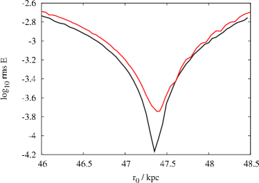
Figure 3.3: Diagnostic quantity $\Delta E/E$ for a range of initial distances, $r_{0}$, for input corresponding to a perfect orbit in the Model II potential. Black line: the procedure performed in the Model II potential. Red line: the procedure performed in a potential with halo asymmetry parameter $q=1$, but otherwise identical to the Model II potential.

The black curve of Fig. 3.3 shows the diagnostic quantity $\Delta E/E$ as a function of initial distance $r_{0}$, where the reconstruction algorithm has been given the correct form of the host potential $\Phi({\bf r})$. As with the reconstruction using radial velocities in Chapter 2, the procedure has highlighted the correct distance to the stream with superb precision. Indeed, in this example, the energy conservation of the best reconstructed trajectory exceeds, by half an order of magnitude, the energy conservation of the equivalent track when reconstructed from radial velocity data. The reasons for this are twofold. Firstly, the upgraded technique of beginning the integration from the centre of the track has reduced numerical noise slightly. Secondly, the two reconstruction techniques, while intellectually equivalent, are mathematically distinct, and it is understandable that one technique may fare better than another, given otherwise identical input.

The red curve in Fig. 3.3 is for reconstructions using the same input data as the black curve, but in this case we have asked the algorithm to reconstruct in a potential similar to Model II, but for which the halo asymmetry parameter (Binney & Tremaine, 2008, Table 2.3) has been changed from its Model II value of $q=0.8$ to $q=1.0$. Thus, the algorithm is attempting to reconstruct trajectories using a potential which is less flattened than the truth.

A minimum in the red curve is still very distinct, and the minimum indeed occurs at approximately the correct distance, as can be seen by comparison with the black curve. We understand this, because we have not altered the halo mass, only its shape. Thus, the magnitude of the force at the distance of the stream remains approximately correct. The results of §2.6 showed that the force strongly determines the distance $r_{0}$ at which the optimum trajectory is found. However, the minimum in the red curve shows substantially worse energy conservation than does the black curve, being half an order of magnitude above the noise floor, as determined by the minimum of the black curve. Thus, as in a reconstruction using radial velocities, when given perfect input, the algorithm can successfully diagnose an incorrect potential.

3.4 Conclusions

We have complemented the work of Binney (2008) and Chapter 2 by showing that, given proper motions measured everywhere along a segment of a single orbit, then full phase-space information can be reconstructed for that orbit, just as it can if radial-velocity measurements are known.

However, proper motions are two-dimensional vectors rather than scalars like line-of-sight velocities, and this fact is rather useful. We have found that, in principle, an orbit can be recovered from proper-motion measurements on purely geometric grounds, with no assumptions made about the potential, and no scanning over distances to find dynamical tracks required. Since any orbit so recovered must correspond to an orbit in the correct potential, the latter would be tightly constrained.

We explore this exciting discovery is full detail in Chapter 4. In the work of this chapter, we have chosen to sacrifice some of the diagnostic power of the proper motions by utilizing only their magnitude, and not their direction, which we deem to be the most difficult quantity to measure. The resulting scheme is logically identical to the scheme of Binney (2008) for reconstructing trajectories from radial-velocity data. Just as in the latter, trajectories reconstructed from proper motions are not forced to be dynamical, and we must hunt for those that are, by computing a diagnostic criterion for each candidate trajectory.

Our tests have indicated that reconstructions using proper motion data are at least as potent as are radial-velocity reconstructions when it comes to both isolating dynamical orbits, and diagnosing the potential. However, like with the radial velocity reconstruction, we expect random input errors, and the failure of actual stream tracks to delineate individual orbits, to be destructive of our ability to identify dynamical solutions.

In order to unlock the diagnostic power of streams using proper-motion measurement, it is likely that techniques similar to those presented in Chapter 2 will be necessary, affording the algorithm the ability to detect those dynamical solutions that can be found with constrained modification of its input. In principle, the adaptation of the procedures to the new algorithm ought to be straightforward, given the intellectual similarity between the two sets of reconstruction equations, and given the similarity in our method of implementing them.

However, we will leave this interesting endeavour for future work. Instead, in the following chapter we will revisit our assertion that recovery of the distance to a stream star can proceed from nothing more than measurement of its on-sky coordinates and proper-motion vector.

Chapter 4 Galactic parallax for the tidal stream GD-1

4.1 Introduction

Conventional trigonometric parallax has long been used to calculate accurate distances to nearby stars. The regular nature of the parallactic motion of a star, caused by the Earth’s orbit around the Sun, allows this motion to be decoupled from the intrinsic proper motion of the star in the heliocentric rest-frame. Hence the distance to the star can be calculated. However, the maximum baseline generating such parallaxes is obviously limited to 2AU. For a given level of astrometric precision, this imposes a fundamental limit to the observable distance. Indeed, the accuracy of parallaxes reported by the Hipparcos mission data (van Leeuwen, 2007) falls to $20$–$30$ percent at best for distances $\sim\!300\,{\rm pc}$ and only then for the brightest stars. Upcoming astrometric projects such as Pan-STARRS (Kaiser et al., 2002), LSST (Tyson, 2002) and the Gaia mission (Perryman et al., 2001) will achieve similar uncertainty for Sun-like stars as distant as a few kpc, and at fainter magnitudes than was possible with Hipparcos. This extended range will encompass less than 1 percent of the total number of such stars in our Galaxy.

It is clear that it will not soon be possible to calculate distances to many of the stars in our Galaxy with conventional trigonometric parallaxes. Alternative means to compute distances to stars are therefore required. Photometry can be used to estimate the absolute magnitude of a star which, when combined with its observed magnitude, allows its distance to be computed. Unfortunately, all attempts to calculate such photometric distances are hindered by the same problems: obscuration by intervening matter alters both observed magnitude (Vergely et al., 1998) and colour (Schlegel et al., 1998; Drimmel & Spergel, 2001), and it is difficult to model appropriate corrections without a reference distance scale. The effects of chemical composition and age further complicate matters (Jurić et al., 2008). It is therefore difficult to compute photometric distances with an accuracy much better than 20 percent, even for nearby stars, and distances to faint stars are less accurate still (Jurić et al., 2008).

Consequently, there exists a demand for long-range distance measuring tools that can complement the existing tools by overcoming some of their limitations. The work of this chapter, much of which was published in articles by Eyre & Binney (2009a) and Eyre (2010), describes such a tool, which measures distances by utilizing the parallactic motion between a distant star and the Sun, rather than that between a star and the Earth as in conventional parallax.

In the general case, it is not possible to obtain distances this way, because the parallactic motion of the star and its intrinsic proper motion are inextricably mixed up. However, in the special case where the star can be associated with a stellar stream, its rest-frame trajectory can be predicted from the locations of the other associated stars. Using this trajectory, the proper motion in the Galactic rest-frame can indeed be decoupled from the reflex motion of the Sun, and the component of its motion due to parallax can be computed.

In the work of the preceding chapter it was discovered that by measuring the proper-motion vector of a star belonging to a stream, it is possible to directly recover the distance to that star. This discovery is an embodiment of the Galactic parallax effect: since we assume that the peculiar motion of the star is tangent to its stream, any proper motion observed perpendicular to that stream can only be due to the reflex motion of the Sun. If the motion of the Sun in a common rest-frame is already known through alternate means, then a parallax can be computed from this perpendicular motion. A diagram illustrating the effect is shown in Fig. 4.1.

Figure 4.1: An illustration of the Galactic parallax effect. The Sun is at some distance $r$ from a star in a stream. The stream track is oriented perpendicularly to the plane of the diagram. In the rest-frame of the Galaxy, the Sun has a velocity ${\bf v}_{0}$ (marked in red), while the velocity of the stream star points vertically out of the page, consistent with it travelling along the stream. In the heliocentric rest-frame, however, the stream star acquires a velocity component $-{\bf v}_{0}$ (marked in black) in the plane of the diagram, due to the reflex motion of the Sun. Observationally, this reflex motion causes the stream star to acquire a component of proper motion, equal to $v_{0}/r\equiv\Pi v_{0}$ projected onto the plane of the sky, that is perpendicular to the stream track. This is the Galactic parallax effect, and allows $\Pi$ to be calculated if ${\bf v}_{0}$ and the proper motion are known.

Such Galactic parallaxes have the same geometrical basis as conventional trigonometric parallaxes, and as such are free from errors induced by obscuration and reddening. However, the range of Galactic parallax significantly exceeds that of conventional parallax. This is because the Sun orbits about the Galactic centre much faster than the Earth orbits the Sun, and because, unlike with conventional parallax, the Galactic parallax effect is cumulative with continued observation. In realistic cases, for a typically oriented stream, we can expect the Galactic parallax to be observable at nearly 40 times the distance of the equivalent trigonometric parallax, based on 3 years of observations. For increased range, one simply observes over a longer baseline.

This large range means that Galactic parallax might prove a powerful tool to complement conventional parallaxes, and validate other distance measuring tools. It is exciting to note that the capabilities of astrometric projects such as LSST, which will observe the conventional parallax of a G star at a distance of $\sim\!1\,{\rm kpc}$ with 20 percent uncertainty, will put much of the Galaxy in range of Galactic parallax calculations with similar accuracy.

The main restriction on the use of Galactic parallax is the requirement for stars to be part of a stream. However, the continuing discovery of significant numbers of streams (Odenkirchen et al., 2003; Majewski et al., 2003; Yanny et al., 2003; Belokurov et al., 2007; Grillmair, 2006a; Grillmair & Dionatos, 2006; Grillmair & Johnson, 2006; Grillmair, 2009; Newberg et al., 2009) using optical surveys implies that they are a staple feature of the Galactic environment, rather than a rarity. The deep surveys of Pan-STARRS and LSST are likely to find yet more, increasing the number of applications for Galactic parallax.

The remainder of this chapter explores the viability of using Galactic parallax to estimate distances and demonstrates its practicality by applying it to data for the GD-1 stream (Grillmair & Dionatos, 2006) published by Koposov et al. (2010, herein K10); we choose to work with the latter over the earlier analysis of the same stream by Willett et al. (2009) on account of the significantly smaller proper-motion uncertainties ($1\,{\rm mas}\,{\rm yr}^{-1}$ vs $4\,{\rm mas}\,{\rm yr}^{-1}$) cited in the later work. Throughout the chapter, the Solar motion is assumed to be

$$(U,V,W)=(10.0,252,7.1)\pm(0.3,11,0.34)\,{\rm km}\,{\rm s}^{-1},$$

consistent with Aumer & Binney (2009), Reid & Brunthaler (2004) and Gillessen et al. (2009).

The chapter is arranged as follows. §4.2 outlines the calculation of Galactic parallax from observational data. §4.3 examines how uncertainties affect Galactic parallax calculations, and §4.4 discusses the practicality of using Galactic parallax as a distance measuring tool in light of those findings. §4.5 demonstrates the use of Galactic parallax on pseudo-data, and shows that our uncertainty estimates are correct, and that the technique is practical. §4.6 uses Galactic parallax to find distances to the tidal stream GD-1. §4.7 presents our concluding remarks.

4.2 Galactic parallax

Suppose that a star is part of a stellar stream, and has a location relative to the Sun described by $({\bf x}-{\bf x}_{0})=r\hat{{\bf r}}$, where $r$ is the distance to the star, and ${\bf x}_{0}$ is the position of the Sun. In the plane of the sky, let the tangent to the trajectory of the stream, near the star, be indicated by the vector $\hat{{\bf p}}$. Assume the velocity of the Sun, ${\bf v}_{0}$, in the Galactic rest-frame (grf) is known, and for the time being assume that streams perfectly delineate orbits. Chapter 3 showed that if the measured proper motion of the star is $\mu\hat{{\bf t}}$, then (equation 3.7)

$$\dot{u}\hat{{\bf p}}=\mu\hat{{\bf t}}+\frac{{\bf v}_{s}}{r}=\mu\hat{{\bf t}}+\Pi{\bf v}_{s},$$ (4.1)

where $\Pi\equiv 1/r$ is the Galactic parallax, $\dot{u}$ is the proper motion as would be seen from the grf, and ${\bf v}_{s}$ is the Sun’s velocity projected onto the plane of the sky. We note that $\dot{u}=v_{t}/r$, where $v_{t}$ is that component of the star’s grf velocity perpendicular to the line of sight, and that

$${\bf v}_{s}=({\bf v}_{0}-\hat{{\bf r}}\cdot{\bf v}_{0}\,\hat{{\bf r}}).$$ (4.2)

Equation (4.1) is a vector expression and can be solved simultaneously for both $\dot{u}$ and $\Pi$ provided that $\hat{{\bf p}}$, $\hat{{\bf t}}$ and ${\bf v}_{s}$ are not parallel. The stream direction $\hat{{\bf p}}$ will not typically be known outright, but must be estimated from the positions of stream stars on the sky. We can achieve this by fitting a low order curve through the position data, the tangent of which is then taken to be $\hat{{\bf p}}$. The curve must be chosen to reproduce the gross behaviour of the stream, but we must avoid fitting high-frequency noise, because $\hat{{\bf p}}$ is a function of the derivative of this curve, which is sensitive to such noise.

4.3 Uncertainty in Galactic parallax calculations

We begin by taking the cross-product of equation (4.1) with $\hat{{\bf p}}$ in order to eliminate $\dot{u}$, and we render the resulting equation into an orthogonal on-sky coordinate system, whose components are denoted by $(x,y)$. Re-arranged for $\Pi$, we find

$$\Pi={{\mu\left(t_{x}\sin\alpha-t_{y}\cos\alpha\right)}\over{v_{s,y}\cos\alpha-v_{s,x}\sin\alpha}},$$ (4.3)

where the $(x,y)$ suffixes denote the corresponding components of their respective vectors, and where we have defined the angle $\alpha\equiv\arctan(p_{y}/p_{x})$.

The choice of coordinates $(x,y)$ is arbitrary. We are therefore free to choose the coordinate system in which $\alpha=0$, i.e. that system in which the $x$-axis points along the stream trajectory, $\hat{{\bf p}}$. Equation (4.3) becomes

$$\Pi=-{\mu t_{\perp}\over v_{s\perp}},$$ (4.4)

where we now identify the $y$-component of the various vectors as that component perpendicular ($\perp$) to the stream trajectory, and the $x$-component as that component parallel ($\parallel$) to the trajectory. Equation (4.4) shows explicitly that the Galactic parallax effect is due to the reflex motion of stream stars perpendicular to the direction of their travel.

Uncertainties in the $(x,y)$ components of the measured quantities $\mu\hat{{\bf t}}$ and ${\bf v}_{s}$, and uncertainty in $\alpha$, can be propagated to $\Pi$ using equation (4.3). When we set $\alpha=0$, this equation becomes

$${\sigma^{2}_{\Pi}\over\Pi^{2}}={\sigma_{\mu}^{2}\over\mu^{2}t_{\perp}^{2}}+{\sigma_{v_{s\perp}}^{2}\over v_{s\perp}^{2}}+{\sigma_{\alpha}^{2}\over v_{s\perp}^{2}}\left(v_{s\parallel}+{\mu t_{\parallel}\over\Pi}\right)^{2},$$ (4.5)

where we anticipate the uncertainty in $\mu\hat{{\bf t}}$ to be isotropic, and so we have set $\sigma_{\mu t_{x}}=\sigma_{\mu t_{y}}=\sigma_{\mu}$.

We assume $\sigma_{\mu}$ to be known from observations; it may contain any combination of random and systematic error. $\sigma_{v_{s\perp}}$ is calculated directly from the error ellipsoid on ${\bf v}_{0}$, which is assumed known. Any error on ${\bf v}_{0}$ affects all data in exactly the same way. However, the projection of error on ${\bf v}_{0}$ to ${\bf v}_{s}$ varies with position on the sky. Hence, the effect of $\sigma_{{\bf v}_{s}}$ is to produce a systematic error in reported distance that varies along the stream in a problem-specific way.

Uncertainty in $\alpha$ arises from three sources. Firstly, a contribution $\sigma_{\alpha,m}$ arises due to the possible misalignment of the stream direction with the rest-frame proper motions of the stars. The magnitude of this misalignment is dependent upon both the geometry of the stream and the nature of the host potential, as is detailed extensively in Chapter 5 of this thesis. However, the misalignment is for the most part predictable, given an initial estimate of the stream’s orbit. The tangent vectors $\hat{{\bf p}}$ can therefore be corrected for the most part of this misalignment, and the residual error is expected to be small.

The second contribution arises because the on-sky trajectory $\hat{{\bf p}}$ is chosen by fitting a smooth curve through observational fields, so $\hat{{\bf p}}$ need not be exactly parallel to the underlying stream. Further, since $\hat{{\bf p}}$ depends on the derivative of the fitted curve, it is likely to be much less well constrained for the data points at the ends of the stream than for those near the middle.

We can quantify this effect. At the endpoints, the fitted curve is likely to depart from the stream by at most $\Delta\psi$, the angular width of the stream on the sky. For a low-order curve, this departure is likely to have been gradual over approximately half the angular stream length, $\Delta\theta$, giving a contribution to $\sigma_{\alpha}$ from fitting of

$$\sigma^{2}_{\alpha,f}={4\Delta\psi^{2}\over\Delta\theta^{2}}.$$ (4.6)

The third contribution to $\sigma_{\alpha}$ arises as follows. Since the stream has finite width, at any point, the stars within it have a spread of velocities, corresponding to the spread in action of the orbits that make up the stream. If the stars in a stream show a spread in velocity $(\sigma_{v_{x}},\sigma_{v_{y}})$ about a mean velocity ${\bf v_{t}}=r\dot{u}\hat{{\bf p}}$, this effect contributes

$$\sigma^{2}_{\alpha,v}={1\over v_{t}^{2}}\left(\sigma_{v_{y}}^{2}\cos^{2}\alpha+\sigma_{v_{x}}^{2}\sin^{2}\alpha\right),$$ (4.7)

to the uncertainty in $\alpha$ for a single star. Again we can choose $\alpha=0$, such that $\sigma_{v_{y}}=\sigma_{v\perp}$, the velocity dispersion perpendicular to the stream direction. Equation (4.7) becomes

$$\sigma^{2}_{\alpha,v}={\sigma^{2}_{v\perp}\over v_{t}^{2}}={\sigma^{2}_{v\perp}\over(v\sin\beta)^{2}},$$ (4.8)

where we have introduced $v$, the grf speed of the stream, and $\beta$, the angle of the stream to the line of sight. $\sigma_{v\perp}$ has its origin in the random motions of stars that existed within the progenitor object. In fact, if we assume the stream has not spread significantly in width, then the width and the velocity dispersion (Binney & Tremaine, 2008, §8.3.3) are approximately related by

$${\sigma_{v\perp}\over v}\simeq{w\over R_{\rm p}}={r\Delta\psi\over R_{\rm p}},$$ (4.9)

where $w$ is the physical width of the stream, and $R_{\rm p}$ is the radius of the stream’s perigalacticon. This gives

$$\sigma_{\alpha,v}={r\Delta\psi\over R_{\rm p}\sin\beta}.$$ (4.10)

If secular spread has made the stream become wider over time, then this relation will over-estimate $\sigma_{\alpha,v}$, since $\sigma_{v\perp}/v$ is roughly constant. $\Delta\psi$ therefore represents an upper bound on the true value of $\sigma_{\alpha,v}$ through this relation. This argument also assumes that the stream was created from its progenitor in a single tidal event. Real streams do not form in this way. However, repeated tidal disruptions can be viewed as a superposition of ever younger streams, created from a progenitor of ever smaller $\sigma_{v\perp}$. Equation (4.10) holds for each of these individually. Thus, $\Delta\psi$ remains a good upper bound for $\sigma_{\alpha,v}$ through this relation.

In reality, we do not measure the proper motion of individual stream stars, but rather the mean motion of a field of $N$ stars. The contribution to $\sigma_{\alpha}$ is from the error on this mean. Putting this together with equation (4.6) gives our final expression for $\sigma_{\alpha}$

$$\sigma^{2}_{\alpha}={\sigma^{2}_{\alpha,v}\over N}+\sigma^{2}_{\alpha,f}+\sigma_{\alpha,m}^{2}={r^{2}\Delta\psi^{2}\over NR_{\rm p}^{2}\sin^{2}\beta}+{4\Delta\psi\over\Delta\theta^{2}}+\sigma_{\alpha,m}^{2}.$$ (4.11)

We note that the first term represents a random error, while the second and third terms represent systematic errors that will vary with position down the stream. In general, $\sin\beta$ and $R_{\rm p}$ are a priori unknown. We can infer $\sin\beta$ from radial velocity information, either directly where the measurements exist, or indirectly from Galactic parallax distances. Guessing $R_{\rm p}$ requires assumptions to be made about the dynamics, but in general we expect the ratio $r/R_{\rm p}\simeq 1$ or less.

Explicit evaluation of $\sin\beta$ and $R_{\rm p}$ are not necessary to evaluate the uncertainty if the contribution from $\sigma_{\alpha,v}$ is overwhelmed by the error from fitting, $\sigma_{\alpha,f}$. We can see this will be the case when the number of observed stars per field

$$N>\Big{(}{r\Delta\theta\over 2R_{\rm p}\sin\beta}\Big{)}^{2}.$$ (4.12)

We expect this to be true in almost all practical cases.

4.3.1 Uncertainty in tangential velocity calculations

Equation (4.1) can also be used to solve for $\dot{u}$

$$\dot{u}={\mu(t_{y}+t_{x})+\Pi(v_{s,y}+v_{s,x})\over\cos\alpha+\sin\alpha},$$ (4.13)

which becomes

$$\dot{u}=\mu(t_{\parallel}+t_{\perp})+\Pi(v_{s\parallel}+v_{s\perp})=\mu t_{\parallel}+\Pi v_{s\parallel},$$ (4.14)

when we set $\alpha=0$. Equation (4.13) combined with equation (4.3) can be used to explicitly propagate uncertainties in the measured quantities to $\dot{u}$. When $\alpha=0$, the uncertainty in $\dot{u}$ is

$${\sigma^{2}_{\dot{u}}\over\dot{u}^{2}} = {{\bf v}_{s}^{2}\sigma_{\mu}^{2}\over\mu^{2}(t_{\perp}v_{s\parallel}-t_{\parallel}v_{s\perp})^{2}}+{t_{\perp}^{2}(v_{s\perp}^{2}\sigma_{v_{s\parallel}}^{2}+v_{s\parallel}^{2}\sigma_{v_{s\perp}}^{2})\over v_{s\perp}^{2}(t_{\perp}v_{s\parallel}-t_{\parallel}v_{s\perp})^{2}}$$ (4.15)

$${}-{2t_{\perp}^{2}v_{s\parallel}v_{s\perp}{\rm cov}(v_{s\parallel},v_{s\perp})\over v_{s\perp}^{2}(t_{\perp}v_{s\parallel}-t_{\parallel}v_{s\perp})^{2}}+{v_{s\parallel}^{2}\sigma_{\alpha}^{2}\over v_{s\perp}^{2}}.$$

$\sigma_{v_{s\parallel}}$ and ${\rm cov}(v_{s\parallel},v_{s\perp})$ are calculated directly from the error ellipsoid on ${\bf v}_{0}$, which we have assumed known.

4.4 Practicality of Galactic parallax as a distance measuring tool

Using equation (4.4) to eliminate $\mu t_{\perp}$ from equation (4.5), and taking the dot product of $\hat{{\bf p}}$ with equation (4.1) to simplify the last term, we obtain

$${\sigma^{2}_{\Pi}\over\Pi^{2}} = {1\over v_{s\perp}^{2}}\Big{\{}(r\sigma_{\mu})^{2}+\sigma_{v_{s\perp}}^{2}+(r\dot{u})^{2}\sigma_{\alpha}^{2}\Big{\}}$$ (4.16)

$$= {1\over v_{s\perp}^{2}}\Big{\{}(r\sigma_{\mu})^{2}+\sigma_{v_{s\perp}}^{2}+v^{2}\left({r^{2}\Delta\psi^{2}\over R_{\rm p}^{2}N}+{4\Delta\psi^{2}\over\Delta\Theta^{2}}+{\sigma_{\alpha,m}^{2}\over\sin^{2}\beta}\right)\Big{\}},$$

where we have noted that $r\dot{u}=v_{t}=v\sin\beta$, and we have related the observed stream length, $\Delta\theta$, to the deprojected length, $\Delta\Theta=\Delta\theta/\sin\beta$. We note that the last term is independent of $r$, since $r\Delta\psi=w$, $\Delta\psi/\Delta\Theta$ and $\sigma_{\alpha,m}$ are all constant, and that for a stream of given physical dimension, the uncertainty in $\Pi$ only has dependence upon the angle of the stream $\beta$ in the misalignment term $\sigma_{\alpha,m}$.

What level of uncertainty does equation (4.16) predict, when realistic measurement errors are introduced? The answer to this is dependent upon both the physical properties of the stream $(R_{p},\Delta\psi,\Delta\Theta,v)$ and the geometry of the problem in question $(r,v_{s\perp},\beta)$.

We progress by assuming ‘typical’ values for some of these quantities. The average magnitude of ${\bf v}_{s}$ taken over the whole sky is $v_{0}\,\pi/4$. The average perpendicular component, for a randomly oriented stream, is $2/\pi$ of this value. We therefore assume a typical value for $v_{s\perp}$ of $v_{0}/2\sim 120\,{\rm km}\,{\rm s}^{-1}$. We also assume a typical grf velocity equal to the circular velocity, $v=v_{c}\sim 220\,{\rm km}\,{\rm s}^{-1}$, and a value for the stream angle to the line of sight, $\sin^{2}\beta\sim 0.5$, consistent with a randomly oriented stream.

McMillan & Binney (2010) recently summarised the current state of knowledge of ${\bf v}_{0}$. The uncertainty quoted is typically $\sim\!5$ percent on each of $(U,V,W)$. Correspondingly, we estimate a typical value for the uncertainty $\sigma_{v_{s\perp}}$ of 5 percent of $v_{s\perp}$, or $6\,{\rm km}\,{\rm s}^{-1}$, which is dominated by the error on V.

The GD-1 stream that we consider below is exceptionally thin and long, with $\Delta\psi\sim\!0.1^{\circ}$ and $\Delta\theta\sim\!60^{\circ}$. The Orphan stream (Grillmair, 2006a; Belokurov et al., 2007) is of similar length, but about 10 times thicker. We therefore take $\Delta\psi\sim\!1^{\circ}$, $\Delta\Theta\sim 60^{\circ}$ as typical of the streams to which one would apply this method. If hundreds of stars are observed for each proper motion datum, then equation (4.12) is true for all realistic combinations of $(r,R_{\rm p})$, so we can ignore the contribution of $\sigma_{\alpha,v}$ to $\sigma_{\alpha}$. The contribution from fitting error is $\sigma_{\alpha,f}\simeq 1.9^{\circ}$. The results of Chapter 5 will show that stream misalignment is highly dependent upon the specifics of the problem in question, but we find that in spherical logarithmic potentials, the typical uncertainty due to misalignment $\sigma_{\alpha,m}\ll 1^{\circ}$. If the misalignment were larger, then the results of Chapter 5 could be used to make a correction to the tangent vectors derived from the stream. In either case, the residual errors $\sigma_{\alpha,m}\ll 1^{\circ}$. Hence, we will take $\sigma_{\alpha}\simeq 2^{\circ}$ as our typical value.

The individual SDSS-USNO proper motions (Munn et al., 2004) used by K10 have a random uncertainty $\sigma_{\mu}\sim 4\,{\rm mas}\,{\rm yr}^{-1}$. After averaging over hundreds of stars and accounting for a contribution from non-stream stars, K10 report a random uncertainty of $\sigma_{\mu}\sim 1\,{\rm mas}\,{\rm yr}^{-1}$ on their GD-1 data. For a stream $10\,{\rm kpc}$ distant, with these proper motions and the typical values mentioned, equation (4.16) reports an uncertainty of $\sigma_{\Pi}/\Pi\sim 40$ percent. By far the greatest contribution comes from the first term in equation (4.16), hence, the error on proper-motion measurement is dominating our uncertainty.

To obtain an uncertainty of $\sigma_{\Pi}/\Pi<20$ percent with Munn et al. (2004) proper-motion measurements, we would need to restrict ourselves to streams less than $5\,{\rm kpc}$ distant. $20$ percent error is also possible at $10\,{\rm kpc}$ given optimum problem geometry. This is clearly competitive with the $\sim 20\,{\rm pc}$ at which one could observe a standard trigonometric parallax, with similar accuracy, using astrometry of this quality. However, previous work (Willett et al., 2009, K10) shows that SDSS photometry combined with population models produce distance estimates accurate to $\sim 10$ percent for stars in streams at $8\,{\rm kpc}$. The accuracy of Galactic parallax is therefore not likely to be as good as that of photometric distances for distant streams, using data this poor, unless the problem geometry is favourable.

Proper-motion data from the Pan-STARRS telescope is expected to be accurate to $\sim\!1\,{\rm mas}\,{\rm yr}^{-1}$ for Sun-like stars at $10\,{\rm kpc}$ (Magnier et al., 2008). K10 reduce raw data with accuracy $\sim\!4\,{\rm mas}\,{\rm yr}^{-1}$ to processed data accurate to $\sim\!1\,{\rm mas}\,{\rm yr}^{-1}$, even though the expected proper motion of the stars is of the same size as the errors. It is not unreasonable to expect a similar analysis applied to Pan-STARRS raw data, where the relative error would be much less than unity, to yield processed data accurate to $\sim 0.2\,{\rm mas}\,{\rm yr}^{-1}$. In truth, the ability of Pan-STARRS to detect very faint stars will increase the number of stars identifiable with a stream, and thus reduce the uncertainty in the mean proper motion further than this, but we use $0.2\,{\rm mas}\,{\rm yr}^{-1}$ as a conservative estimate.

The same $10\,{\rm kpc}$ distant stream would have a parallax error of $\sigma_{\Pi}/\Pi\simeq 11$ percent with data this accurate. An error of less than $20$ percent is possible for a typical stream less than $\sim 23\,{\rm kpc}$ distant, and for a stream with favourable geometry less than $50\,{\rm kpc}$ distant. Jurić et al. (2008) report that SDSS photometric distances for dwarf stars have $\sim\!40$ percent error at $20\,{\rm kpc}$. Thus, the accuracy of Galactic parallax derived from Pan-STARRS data should be at least comparable to distance estimates from photometric methods, even in the typical case.

Future projects such as LSST and Gaia will each obtain proper motions accurate to $\sim 0.2\,{\rm mas}\,{\rm yr}^{-1}$ for Sun-like stars $10\,{\rm kpc}$ distant (Ivezić et al., 2008; Perryman et al., 2001). These data would allow a distance estimate for our typical stream accurate to $8$ percent, and a stream with favourable geometry accurate to $4$ percent. Error in the proper motion no longer dominates the uncertainty in these calculations. We might expect such accurate astrometric surveys to reduce the uncertainty in the Solar motion; in this case, the error in Galactic parallax would be lower still.

Gaia will not observe Sun-like stars beyond $10\,{\rm kpc}$, but LSST will, with accuracy of $0.4\,{\rm mas}\,{\rm yr}^{-1}$ for dwarf stars $30\,{\rm kpc}$ distant (Ivezić et al., 2008). The accuracy of the parallax to our typical stream at this distance would be about $14$ percent with these data, and $6$ percent is achievable with optimum geometry. A typical stream could be measured to 20 percent accuracy out to $40\,{\rm kpc}$, and a stream with favourable geometry out to $54\,{\rm kpc}$; this range approaches the limit of LSST’s capability for detection of dwarf stars. Such data will put the Orphan stream, which is about $20-30\,{\rm kpc}$ distant (Grillmair, 2006a; Belokurov et al., 2007; Sales et al., 2008), in range of accurate trigonometric distance estimation. For comparison, photometric distances from SDSS data are hardly more accurate than 50 percent for this stream (Belokurov et al., 2007).

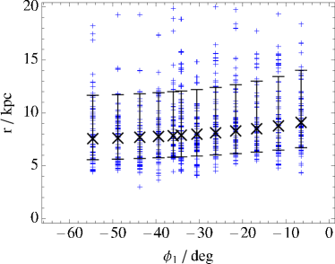
Figure 4.2: Crosses: Galactic parallax distances computed from the pseudo-data, with no extraneous errors. Error bars: the random scatter expected in Galactic parallax distances, with measurement errors as mentioned in the text. Plus signs: Galactic parallax distances computed from 60 Monte Carlo realisations of each pseudo-datum convolved with the measurement errors. The analytic uncertainty estimate and the Monte Carlo realisations are in good agreement.

4.5 Tests of Galactic parallax

To test the method, pseudo-data were prepared from an orbit fitted to data for the GD-1 stream by K10. The orbit is described by the initial conditions

$${\bf x}=(-3.41,13.00,9.58)\,{\rm kpc},\qquad{\bf v}=(-200.4,-162.6,13.9)\,{\rm km}\,{\rm s}^{-1},$$

where the $x$-axis points towards the Galactic centre, and the $y$-axis points in the direction of Galactic rotation. The orbit was integrated in the logarithmic potential

$$\Phi(x,y,z)={v_{c}^{2}\over 2}\log\left(x^{2}+y^{2}+\left({z\over q}\right)^{2}\right),$$ (4.17)

where $v_{c}=220\,{\rm km}\,{\rm s}^{-1}$ and $q=0.9$. The resulting trajectory was projected onto the sky, assuming a Solar radius $R_{0}=8.5\,{\rm kpc}$. The implicit assumption is made that the GD-1 stream is closely approximated by an orbit: the work of Chapter 5 will show that this assumption is a fair one. Several points were sampled from the on-sky track, and each was taken to be a separate datum in the pseudo-data set. The proper motion for each datum was computed by projecting the difference between its grf motion and the Solar motion onto the sky.

The pseudo-data were transformed into the rotated coordinate system used by K10 to facilitate comparison with their data; the transformation rule is given in the appendix to K10. The stream is very flat in this coordinate system, so the dependence of $\phi_{2}$ on $\phi_{1}$ is relatively weak. This helps to increase the quality of the fitted curve and minimises the corresponding error in $\sigma_{\alpha,f}$.

To simulate the observed scatter in the real positional data, the pseudo-data were each scattered in the $\phi_{2}$ coordinate according to a randomly-sampled Gaussian distribution with a dispersion $\sigma_{\phi_{2}}=0.1^{\circ}$. The resulting positional pseudo-data are plotted in Fig. 4.3, along with the orbit from which they were derived (full curve). A cubic polynomial representing $\phi_{2}(\phi_{1})$ was least-squares fitted to the pseudo-data, the tangent of which was used to estimate $\hat{{\bf p}}$. In the case of the pseudo-data, uniform weights were applied to each datum for the fitting processes. The resulting curve is also shown in Fig. 4.3 (dotted curve).

Figure 4.3: Full line: the orbit for the GD-1 stream, taken from K10. Crosses: pseudo-data derived from that orbit, but randomly scattered in $\phi_{2}$ according to a Gaussian distribution with a dispersion of $\sigma_{\phi_{2}}=0.1^{\circ}$. Dotted line: a cubic polynomial fitted to the pseudo-data, used to estimate stream direction.

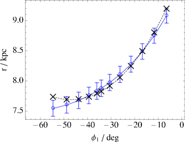
Figure 4.4: Dotted line: the orbit of the GD-1 stream, taken from K10. Crosses: the true distance of each pseudo-datum. Circles: Galactic parallax distances computed from the pseudo-data. The error bars represent the distance error expected from the polynomial fitting procedure. No extraneous error was added. The error bars are shown to be a good estimate of likely error from the fitting procedure, and the agreement of the distances overall is excellent.

When the correct orbit is used to calculate $\hat{{\bf p}}$, and precise values for the measured proper motion $\mu\hat{{\bf t}}$ and Solar reflex motion ${\bf v}_{s}$ are used, the distance is recovered perfectly from equation (4.4). Fig. 4.4 compares the recovered distance when $\hat{{\bf p}}$ is estimated using the polynomial fit to the pseudo-data, but still using accurate values for $\mu\hat{{\bf t}}$ and ${\bf v}_{s}$. Our pseudo-data stream is $\Delta\psi\simeq 0.1^{\circ}$ wide and $\Delta\theta\simeq 60^{\circ}$ long. Equation (4.6) therefore estimates $\sigma_{\alpha,f}\simeq 0.38^{\circ}$. The recovered distances in Fig. 4.4 are in error by only $\sim 2$ percent across most of the range, which is the approximate uncertainty predicted by equation (4.5) for this value of $\sigma_{\alpha,f}$. Thus, the estimation of $\hat{{\bf p}}$ from the observed stream is good, and contributes little error to the distance calculations.

The K10 observational data for the GD-1 stream, discussed below, have a similar uncertainty $\sigma_{\alpha}\sim 0.38^{\circ}$ due entirely to the fitting process, and proper-motion uncertainties $\sigma_{\mu}\sim 1\,{\rm mas}\,{\rm yr}^{-1}$. Fig. 4.2 shows the recovered distances from Fig. 4.4 with error bars for the expected uncertainty in recovered distance, given these measurement uncertainties and the uncertainty in ${\bf v}_{0}$ quoted in §4. Also plotted for each datum are the distances recovered from 60 Monte Carlo realisations of the pseudo-data input values, convolved with the errors given above.

Equation (4.5) is found to be a good estimator for the uncertainty, with approximately 80 percent of the Monte Carlo realisations falling within the error bars. The error in parallax for the K10 data is thus predicted to be about 50 percent, of which the greatest contribution comes from the uncertainty in proper motion.

4.6 Distance to the GD-1 stream

Figure 4.5: Crosses: on-sky position data for the GD-1 stream, as published in K10. The error bars represent the quoted uncertainties. Full line: linear least-squares fit of a cubic polynomial, $\phi_{2}(\phi_{1})$, to these data; the inverse-square of the uncertainties was used to weight the fit.

Fig. 4.5 shows the on-sky position data for the GD-1 stream, as published in K10. Also shown in Fig. 4.5 is a linear least-squares fit of a cubic polynomial to these data, used to estimate $\hat{{\bf p}}$. The weights for the fit were the inverse-square uncertainties for each position field, as given by K10.

K10 provide measured proper-motion data for five fields of stars, spanning the range $\phi_{1}\sim(-55,-15)^{\circ}$, along with uncertainties for these measurements. The uncertainty in ${\bf v}_{s}$ is computed for each individual field from the uncertainty in ${\bf v}_{0}$ given in §4. Uncertainty in the stream direction is $\sigma_{\alpha}\sim 0.38^{\circ}$, which is entirely contributed by the curve fit to the stream; since hundreds of stars contributed to the calculation of the proper motions, the contribution from the first term in equation (4.11) is negligible. We have also assumed that the contribution to $\sigma_{\alpha}$ from stream misalignment is negligible. This assumption is validated by the results of Chapter 5, which predicts that the projection of GD-1 should be perfectly aligned with the orbits of its stars.

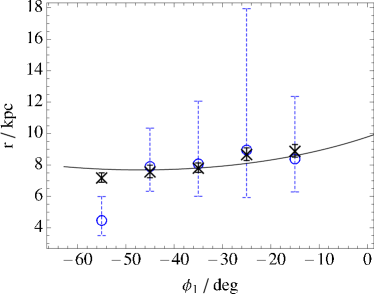
Figure 4.6: Circles: Galactic parallax distances for the GD-1 data presented in K10. Dotted error bars: the uncertainty estimated by equation (4.5), given the K10 measurement uncertainties. Crosses: the photometric distances reported in K10, along with their error bars. Full line: the orbit for GD-1 taken from K10. With the exception of the datum at $\phi_{1}\sim-55$ deg, the Galactic parallax distances are in excellent agreement with the photometric distances from K10. The dotted error bars appear to seriously over-estimate the true error in the distance estimates.

Fig. 4.6 shows the Galactic parallax distances for each of these data, along with the K10 photometric distances. The dotted error bars represent the expected error in distance for the uncertainties given. The small solid error bars are the uncertainties reported by K10 for their photometric distances. The K10 orbit used to compute the earlier pseudo-data is plotted for comparison.

With the exception of the datum at $\phi_{1}\sim-55^{\circ}$, the parallax distances and the K10 distances are in remarkable agreement. However, the dotted error bars vastly overestimate the true error in the results. If we ignore the datum at $\phi_{1}\sim-55^{\circ}$, the scatter in the distance, $\sigma_{r}\sim 1\,{\rm kpc}$, is similar to that of the photometric distances, and consistent with a true random error of $\sigma_{\mu}\sim 0.3\,{\rm mas}\,{\rm yr}^{-1}$, and negligible systematic offset. We cannot explain this discrepancy, except by suggesting that the K10 proper-motion measurements are more accurate than the published uncertainties suggest. This is corroborated by the top-right panel of Fig. 13 from K10 in which the $\mu_{\phi_{2}}$ data, with the exception of the datum at $\phi_{1}\sim-55^{\circ}$, show remarkably little scatter within their error bars.

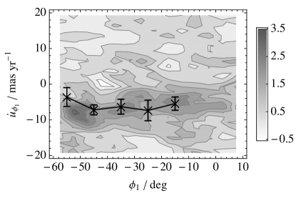
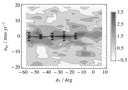
Figure 4.7: Full lines: Galactic rest-frame proper motion, $\dot{u}$, calculated from the K10 data using equation (4.14). The (left, right) panels show the $(\phi_{1},\phi_{2})$ components respectively. Plotted in the background are the observational data from Fig. 9 in K10; the greyscale shows the number of stream stars, per bin, with the given motion. The data are broadly consistent, except for the datum at $\phi_{1}\sim-55$ deg in the left panel.

Fig. 4.7 shows the Galactic rest-frame proper motions, $\dot{u}$, calculated from equation (4.14) along with their error bars, from equation (4.15). In the background are plotted the data from Fig. 9 of K10, which show the density of stars with a given grf proper motion in the sample of stars chosen to be candidate members of the stream, and after subtraction of a background field. The K10 grf proper motions have been calculated by correcting measured proper motion for the solar reflex motion, using an assumed distance of $8\,{\rm kpc}$ (Koposov, private communication); this assumption will cause a systematic error in the K10 proper motions, of order the distance error, which changes with position down the stream. The apparently large width of the stream in this plot is due to uncertainty in the underlying Munn et al. (2004) proper-motion data.

The stream is clearly visible in this plot as the region of high density spanning $\phi_{1}\sim(0,-60)^{\circ}$ with $\dot{u}_{\phi_{2}}\simeq 0\,{\rm mas}\,{\rm yr}^{-1}$ and $\dot{u}_{\phi_{1}}$ falling slowly between $(-6,-10)\,{\rm mas}\,{\rm yr}^{-1}$. Despite the expected systematic error, the estimates of $\dot{u}$ from the parallax calculation are consistent with these data, with the exception of the same datum at $\phi_{1}\sim-55^{\circ}$ that also reports an anomalous distance.

We explain this suspect datum as follows. From inspection of the top-right panel of Fig. 13 from K10, it is apparent that the $\mu_{\phi_{2}}$ measurement for this datum is not in keeping with the trend. Conversely, the corresponding $\mu_{\phi_{1}}$ measurement is not obviously in error. If the magnitude of $\mu_{\phi_{2}}$ for this datum has been over-estimated by the K10 analysis, then equation (4.4) will over-estimate the parallax, and hence under-report the distance. Fig. 4.6 indicates that the distance for this datum is indeed under-reported.

The effect of such an error in $\mu_{\phi_{2}}$ on the grf proper-motion, $\dot{u}$, can be understood by considering equation (4.14). If $\Pi$ is over-estimated, $\dot{u}$ will be either over-estimated or under-estimated, depending on the relative sign of the two terms. In the case of GD-1, $\mu t_{\parallel}$ and $v_{s\parallel}$ have opposite signs, so an over-estimated $\Pi$ will result in an under-estimated $\dot{u}$. This too corresponds with the behaviour of the suspect datum in Fig. 4.7.

It is unknown why this particular datum should be significantly in error while the other data are not. There are no obvious structures in the lower panel of Fig. 4.7 which might cause the fitting algorithm in K10 to mistakenly return an incorrect value for $\mu_{\phi_{2}}$. Nonetheless, if the scatter in the other data are accepted as indicative of their true statistical error, it is clear that the datum at $\phi_{1}\sim-55^{\circ}$ cannot represent the proper motions of GD-1 stars at that location. We therefore predict that an appropriate re-analysis of the proper-motion data, taking care to ensure that a signal from GD-1 stream stars is properly detected, will return a revised proper-motion of $\mu_{\phi_{2}}\sim-3\,{\rm mas}\,{\rm yr}^{-1}$.

In summary, it seems that Galactic parallax measurements confirm the K10 photometric analysis, and predict that the stream is approximately $(8\pm 1)\,{\rm kpc}$ distant, where the uncertainty denotes the scatter in the results. Since Galactic parallax and photometric estimates are fundamentally independent, it seems unlikely that systematic errors in either would conspire to produce the same shift in distance; this suggests that no systematic error is present.

We also calculate a grf proper motion for the stream of $\dot{u}_{\phi_{1}}=(-7\pm 2)\,{\rm mas}\,{\rm yr}^{-1}$, corresponding to a grf tangential velocity of $(265\pm 80)\,{\rm km}\,{\rm s}^{-1}$ in a direction $(\dot{u}_{l}\cos b,\dot{u}_{b})\simeq(0.8,-0.6)$. This implies that the stream is on a retrograde orbit, inclined to the Galactic plane by $\sim\!37^{\circ}$, which is in accordance with previous results (Willett et al., 2009; Koposov et al., 2010).

The galactocentric radius of $\sim\!14.5\,{\rm kpc}$ does not seem to be changing rapidly along the stream’s length, which subtends $\sim\!12^{\circ}$ when viewed from the Galactic centre. This implies that the observed stream is at an apsis. The grf velocity of the stream is faster than the circular velocity, $v_{c}\sim 220\,{\rm km}\,{\rm s}^{-1}$. This implies that the stream is at pericentre, although the large uncertainty prevents a firm conclusion from being drawn. We note that the radial velocity data in K10 would also imply that the stream is observed at pericentre.

4.7 Conclusions

In this chapter, we have demonstrated the practical application of a technique for computing distances using Galactic parallax. This technique utilises the predictable trajectories of stars in a stream to identify the contribution of the reflex motion of the Sun to the observed proper motion. The parallax and the Galactic rest-frame proper motion follow from this.

Galactic parallax is a geometric phenomenon, and the distances obtained from it are in every way as fundamental as those obtained using conventional trigonometric parallax. The only assumption made is knowledge of the Galactic rest-frame velocity of the Sun. It is also a requirement that the observed stars are part of a stream. Recent evidence (Odenkirchen et al., 2003; Majewski et al., 2003; Yanny et al., 2003; Belokurov et al., 2007; Grillmair, 2006a; Grillmair & Dionatos, 2006; Grillmair & Johnson, 2006; Grillmair, 2009; Newberg et al., 2009) indicates that tidal streams are a common constituent of the Galactic halo, and so this technique should have widespread application.

The key hurdle to the widespread application of this technique is the lack of high-accuracy proper-motion data for distant stream stars. Given the advent of next-generation astrometric projects such as Pan-STARRS (Kaiser et al., 2002), LSST (Tyson, 2002) and Gaia (Perryman et al., 2001), proper-motion catalogues with billions of entries of the required precision will become available in the next few years. The technique should then become the standard method of determining the distance to remote stream stars.

4.7.1 Summary

We have presented a method for calculating the Galactic parallax of tidal streams. We first determine the on-sky direction of the stream by fitting it with a curve. We then combine the tangents of this curve with measured proper-motion data to estimate the parallax of the stream.

We have derived an expression for the uncertainty in Galactic parallax calculations. We include contributions from measurement errors in proper motion and the Solar motion, error in the estimation of stellar trajectories from the stream direction, and algorithmic error in the estimation of stream direction itself.

The uncertainty for calculations involving a particular stream depends upon the size, location and orientation of the stream, as well as upon measurement errors. We estimate that using individual proper motions accurate to $4\,{\rm mas}\,{\rm yr}^{-1}$, available now in published surveys (Munn et al., 2004), the parallax of a $10\,{\rm kpc}$ distant stream with typical geometry can be measured with an uncertainty of 40 percent. The parallax of a stream with optimum geometry could be measured with approximately half this uncertainty.

Proper-motion data from the forthcoming Pan-STARRS PS-1 survey (Kaiser et al., 2002; Magnier et al., 2008) will yield the distance to a typical $10\,{\rm kpc}$ distant stream with 11 percent accuracy, or the distance to a stream at $23\,{\rm kpc}$ with 20 percent accuracy; with favourable geometry this accuracy could be achieved for a stream as distant as $50\,{\rm kpc}$. With data of this quality, the uncertainty in distances from Galactic parallaxes will be considerably lower than those of photometric distances to remote streams.

The LSST (Tyson, 2002; Ivezić et al., 2008) and the Gaia mission (Perryman et al., 2001) will produce proper-motion data that are more accurate still. Such data would allow the distance to stars in a $10\,{\rm kpc}$ typical stream to be computed to an accuracy of order of 8 percent, where the limitation is now imposed by uncertainty in the solar motion and in the stream trajectory. It is likely that LSST and Gaia data will allow the uncertainty in the solar motion to be significantly reduced, so in reality much better precision can be expected at this distance. For streams $30\,{\rm kpc}$ distant, LSST proper motions will allow distance estimates as accurate as 14 percent to be made in the typical case, and 6 percent with optimum geometry. Thus, the high-quality astrometric data that is expected to be available in the next decade will allow parallax estimates for very distant streams to be made with unparalleled accuracy.

To test the method presented, we have created pseudo-data simulating the GD-1 stream (Grillmair & Dionatos, 2006). When the method is provided with error-free pseudo-data, the correct parallax is computed perfectly. When errors are introduced into the pseudo-data, the reported parallax degrades in line with the uncertainty estimates.

We applied the method to the astrometric data for the GD-1 stream in Koposov et al. (2010). With the exception of a single datum, the Galactic parallax is remarkably consistent with the photometric distances quoted by Koposov et al. (2010). Indeed, the uncertainty in the measured proper motions quoted by Koposov et al. (2010) should produce significant error in the Galactic parallax. However, the scatter in the results is consistent with a random error of only $\sim 0.3\,{\rm mas}\,{\rm yr}^{-1}$, and if the photometric distances of K10 are believed, no systematic offset. This is at odds with the typical uncertainty in the proper motion of $\sim 1\,{\rm mas}\,{\rm yr}^{-1}$ reported by Koposov et al. (2010). We cannot explain this discrepancy, other than to suggest that the Koposov et al. (2010) method for estimating error in the proper motions is producing significant over-estimates.

The Galactic rest-frame proper motions predicted for the stream are also consistent with observational data from Koposov et al. (2010), with the exception of the same datum that also reports an inconsistent distance. We conclude that the proper-motion associated with this datum is erroneous, and we predict that reanalysis of the stream stars near this datum will reveal a reduced proper-motion measurement of $\mu_{\phi_{2}}\sim 3\,{\rm mas}\,{\rm yr}^{-1}$.

Photometry and Galactic parallax produce fundamentally independent estimates of distance. The quality of the corroboration of the Koposov et al. (2010) photometric distance estimates for GD-1 by the Galactic parallax estimates presented here therefore lends weight to the conclusion that the predicted distance, in both cases, is correct. On this basis, we conclude that the GD-1 stream is about $(8\pm 1)\,{\rm kpc}$ distant from the Sun, on a retrograde orbit that is inclined $37^{\circ}$ to the Galactic plane with a rest-frame velocity of $(265\pm 75)\,{\rm km}\,{\rm s}^{-1}$. We also conclude that the visible portion of the stream is probably at pericentre.

4.7.2 Future directions

The prospect of being able to map trigonometric distances in the Galaxy to high accuracy at a range of tens of kiloparsecs is indeed exciting. The distances generated using this method, although limited to stars in streams, could be used to calibrate other distance measuring tools, such as photometry, that would be more widely applicable. The technique is immediately applicable to any stream for which proper-motion data are currently available, although we anticipate limited accuracy until better proper-motion data are available.

Given enough parallax data points along a given stream, an orbit can be constructed by connecting those points. This orbit is predicted independently of any assumption about the Galactic potential, which it must strongly constrain. Constraints on the Galactic potential impose constraints on theories of galaxy formation and cosmology. It would seem that the combination of dynamics and Galaxy-scale precision astrometry, such as provided by this method, could well have profound implications for astrophysics in the future.

At present, however, it is not obvious how to combine all sources of astrometric and dynamical information, to produce the tightest constraints on the potential. A significant theoretical effort is therefore required to explore methods for combining this information, in anticipation of the arrival of higher quality astrometric data in the next few years.

Chapter 5 The mechanics of streams

5.1 Introduction

Many of the techniques used to harness the diagnostic power of tidal streams rely upon the assumption that such streams delineate orbits precisely (Binney, 2008; Eyre & Binney, 2009a; Odenkirchen et al., 2009; Willett et al., 2009; Koposov et al., 2010; Eyre, 2010).

Although both the author (Chapter 2; Eyre & Binney, 2009b) and others (Dehnen et al., 2004; Choi et al., 2007; Montuori et al., 2007) have shown evidence that this is not necessarily the case, there has not to date been an exposition of how streams form that fundamentally addresses this issue. In particular, it is necessary to understand under what circumstances tidal streams delineate orbits, by what measure they are in error when they do not, and what can be done to correct this error.

The few studies that have been made have either focused on N-body simulations (e.g. Choi et al., 2007; Montuori et al., 2007), the confusion of which makes the predominant physics hard to isolate, or have attempted to describe the problem in terms of conventional phase-space coordinates and classical integrals (e.g. Dehnen et al., 2004; Choi et al., 2007), which makes the problem intractably hard. In particular, the work of Choi et al. (2007) made some progress towards understanding the dynamical structure of clusters at the point of disruption, and they provide a qualitative picture of the evolution of tidal tails, understood in terms of classical integrals. However, they are unable to make predictions for stream tracks on the basis of this picture alone, and they are ultimately forced to rely on N-body simulation. In the work of this chapter, we approach the problem using action-angle variables (Binney & Tremaine, 2008, §3.5), in which the physics of stream formation turns out to have a natural and simple expression.

We confine our investigation to the formation of long, cold streams, such as may form from tidally disrupted globular clusters. We do so for two reasons. Firstly, a low mass for the progenitor cluster simplifies the understanding of its orbital mechanics, because of the lack of tidal friction and other feedback effects in their interaction with the host galaxy. Secondly, thin, long streams provide the strongest constraints upon the Galactic potential (Chapter 2; Binney, 2008; Eyre & Binney, 2009b), because any orbit delineated by them can be observationally identified with less ambiguity. It is therefore long, cold streams that are of primary interest for use in probing the potential.

We study the mechanics of stream formation immediately following the tidal disruption of a progenitor cluster. In most of the work that follows, the assumption is made that stream stars feel only the potential of the Galaxy; i.e. the stream stars do not self-gravitate. This assumption is generally a fair one: the stars in streams are generally spaced too widely for their self-gravity to be of consequence (Dehnen et al., 2004). Indeed, we will demonstrate in §5.6.2 below that self-gravity becomes negligible shortly after stars are stripped from the cluster.

The chapter is arranged as follows: The remainder of this introduction discusses the action-angle variables in which we perform our analysis. §5.2 discusses the basic mechanics of stream formation and propagation. §5.3 discusses the detail of stream formation in spherical systems, and explores some examples. §5.4 describes the principles and pitfalls of mapping streams from action-angle space to real-space. §5.5 describes the consequences of optimizing potential parameters by assuming that streams follow orbits. §5.6 examines the action-space distribution of disrupted clusters using N-body simulation. §5.7 discusses stream formation in flattened systems, using oblate axisymmetric Stäckel potentials as an example. Finally, §5.8 presents our concluding remarks.

5.1.1 Action-angle variables

We will approach the analysis of stream formation and propagation by describing the problem using action-angle variables. The usefulness and theoretical basis of action-angle variables is extensively discussed in §3.5 of Binney & Tremaine (2008). Here, we merely note that action-angle variables are a set of canonical coordinates, like conventional phase-space coordinates, that can be used to describe systems in Hamiltonian mechanics.

The coordinates are special because the canonical momenta, called actions, ${\bf J}$, are integrals of the motion, and are thus constant with the passage of time. The equation of motion for ${\bf J}$ then reads

$$\dot{J_{i}}=0=-{\partial H\over\partial\theta_{i}},$$ (5.1)

where we have introduced the angle variables, $\theta$. Equation (5.1) requires that the Hamiltonian, $H({\bf J})$ be independent of $\theta$, and therefore a function of ${\bf J}$ only. The equation of motion for $\theta$ is then,

$$\dot{\theta_{i}}={\partial H\over\partial J_{i}}\equiv\Omega_{i}({\bf J}),$$ (5.2)

where the frequencies $\mbox{\boldmath$\theta$}({\bf J})$, being functions of ${\bf J}$ only, are constant. The solution to equation (5.2) is very simple

$$\mbox{\boldmath$\theta$}(t)=\mbox{\boldmath$\theta$}(0)+{\bf\Omega}\,t.$$ (5.3)

Hence, the motion of a system described by action-angle variables is very easy to predict. Moreover, because the actions for the system are constant, any approximation that we may make to $H({\bf J})$, if valid at one time, is automatically valid at all times. This particular feature is of critical importance in simplifying the analysis of the propagation of streams in the work that follows.

§3.5 of Binney & Tremaine (2008) discusses at length the calculation of action-angle coordinates in various systems. Here, we note that standard methods for calculating action-angle coordinates require the Hamilton-Jacobi equation (equation 3.205, Binney & Tremaine, 2008) to separate. This condition is met by all spherically symmetric potentials, but excludes any asymmetric potential that is not of Stäckel form (see §5.7.2 below). Given this condition, the action corresponding to a coordinate $q$ is given by

$$J_{q}={1\over 2\pi}\oint p_{q}\,dq,$$ (5.4)

where the integral is over the closed path that encloses a single oscillation of the coordinate $q$ along an orbit.

We note that just as spherical systems are naturally described by spherical polar coordinates $(r,\vartheta,\phi)$, the natural actions for such systems are $(J_{r},L)$, where $L$ is the angular momentum, and we have without loss of generality confined our motion to the $(x,y)$ plane. We can qualitatively understand the meaning of these actions. An orbit with finite $L$ we understand to be circular at, or to oscillate in epicycles around, some guiding-centre radius $r_{g}$. An orbit with $J_{r}=0$ always has zero radial momentum, and thus corresponds to a circular orbit. Conversely, an orbit with comparatively large $J_{r}$ must be very eccentric. Hence, $J_{r}$ quantifies the radial motion of an orbit, while $L$ quantifies its azimuthal motion. We note for completeness that orbits with $L=0$ are plunging orbits.

In the sections that follow, we utilize the equations from §3.5.2 of Binney & Tremaine (2008) to transform between the action-angle coordinates $(J_{r},L,\theta_{r},\theta_{\phi})$ and conventional phase-space coordinates, when investigating spherical potentials. The action-angle coordinates used when investigating non-spherical potentials are discussed in §5.7.2 below.

5.2 The formation of streams from tidally stripped clusters

Consider a low-mass cluster, just past the point of disruption, such that the stripped stars no longer feel the effects of its gravity. The cluster is on a regular orbit, identified by its actions ${\bf J}_{0}$, in a fixed background potential, which has a Hamiltonian $H$ in terms of the actions ${\bf J}$. Suppose further that in the locality of ${\bf J}_{0}$, the Hamiltonian is well described by the Taylor expansion,

$$H({\bf J})=H_{0}+{\bf\Omega}_{0}\cdot\delta{\bf J}+{1\over 2}\delta{\bf J}^{T}\cdot{\bf D}\cdot\delta{\bf J},$$ (5.5)

where $\delta{\bf J}={\bf J}-{\bf J}_{0}$, and ${\bf D}$ is the Hessian of $H$

$$D_{ij}=\left.{\partial^{2}H\over\partial J_{i}\,\partial J_{j}}\right|_{\bf J},$$ (5.6)

and ${\bf\Omega}_{0}$ is the frequency of the cluster’s orbit

$$\Omega_{0,i}=\left.{\partial H\over\partial J_{i}}\right|_{\bf J}.$$ (5.7)

The frequency ${\bf\Omega}$ of a nearby orbit ${\bf J}$ is then

$${\bf\Omega}({\bf J})={\bf\Omega}_{0}+{\bf D}\cdot\delta{\bf J}.$$ (5.8)

If the disrupted cluster has some spread in actions $\Delta{\bf J}$ and angles $\Delta\mbox{\boldmath$\theta$}_{0}$, then the spread in angles after some time $t$ is given by (Tremaine, 1999; Binney & Tremaine, 2008, §8.3.1),

$$\Delta\mbox{\boldmath$\theta$}(t)=t\Delta{\bf\Omega}+\Delta\mbox{\boldmath$\theta$}_{0}\simeq t\Delta{\bf\Omega},$$ (5.9)

where the near equality is valid when $\Delta{\bf\Omega}\,t\gg\Delta\mbox{\boldmath$\theta$}_{0}$, and where we have introduced the spread in frequencies, $\Delta{\bf\Omega}$, which are related to the spread in actions via

$$\Delta{\bf\Omega}={\bf D}\cdot\Delta{\bf J}.$$ (5.10)

In the absence of self-gravity, the action-space distribution $\Delta{\bf J}$ is frozen for all time. ${\bf D}$ and ${\bf\Omega}$ are functions of ${\bf J}$ only, and so are similarly frozen. The secular evolution of a disrupted cluster is therefore to spread out in angle-space, with its eventual shape determined by $\Delta{\bf\Omega}={\bf D}\cdot\Delta{\bf J}$, and its size growing linearly with $t$.

For a given $\Delta{\bf J}$, what does $\Delta{\bf\Omega}$ look like? Equation (5.9) and equation (5.10) show that the function of ${\bf D}$ is to act as a linear map between a star’s position in action-space and its position in angle-space. We note that ${\bf D}$ is a Hessian and is therefore symmetric. Associated with ${\bf D}$ are three orthogonal directions, $\hat{{\bf e}}_{n}$ ($n=1,3$), corresponding to the eigenvectors of ${\bf D}$ if it is evaluated as a matrix. Each of these directions is associated with an eigenvalue, $\lambda_{n}$.

Consider a cluster whose stars are distributed isotropically within a unit sphere about some mean ${\bf J}_{0}$ in action-space. The corresponding angle-space structure, resulting from the mapping of this sphere by ${\bf D}$, will be an ellipsoid with semi-axes of length $t\lambda_{n}$ and direction $\hat{{\bf e}}_{n}$.

If the $\lambda_{n}$ are finite and approximately equal, such an isotropic cluster will spread out in angle-space with no preferred direction, with the density initially falling as $t^{3}$. Eventually, the cluster will uniformly populate the whole of angle-space; in real-space the cluster will uniformly fill the entire volume occupied by the orbit ${\bf J}_{0}$. For a cluster disrupting in an actual galaxy, the structure would quickly fall below the level of observability.

If one of the $\lambda_{n}$ is much smaller than the others, then ${\bf D}$ will act to map the cluster into a highly flattened ellipsoid in angle-space. In real-space, the cluster will occupy a 2-dimensional subspace of the orbital volume of ${\bf J}_{0}$. The precise configuration of this subspace is likely to be complex. However, the density will initially fall as $t^{2}$, and in a real galaxy, such a structure will rapidly become invisible.

If two of the $\lambda_{n}$ are small, then ${\bf D}$ acts to map the cluster into a line in angle-space. In this case, the resulting real-space structure will be a filament. The density of this filament will fall linearly with $t$. In a real galaxy, such a structure may therefore persist with a significant overdensity for some time. It is this case that describes the formation of tidal streams (Binney & Tremaine, 2008, §8.3.1), and it is this case that we investigate in detail in this chapter. Finally, if all the $\lambda_{n}$ are zero, there will be no spread at all, and even an unbound cluster will remain intact indefinitely.

We note that there is no a priori reason for any of the $\lambda_{n}$ to be small. The existence of ${\bf D}$ imposes no conditions on $H$ in general, save that it must be twice differentiable near to ${\bf J}_{0}$. We can write a Hamiltonian for which, for particular ${\bf J}_{0}$ at least, the $\lambda_{n}$ and the $\hat{{\bf e}}_{n}$ are arbitrary. It must therefore be a peculiar property of realistic Galactic potentials that causes disrupted clusters to form streams.

Lastly, a word on validity. The Taylor expansion equation (5.5) is valid when,

$$D_{ij}\gg{1\over 3}{\partial D_{ij}\over\partial J_{k}}\delta J_{k}={1\over 3}{\partial^{3}H\over\partial J_{i}\partial J_{j}\partial J_{k}}\delta J_{k}.$$ (5.11)

This condition approximates to

$$\delta J_{i}\ll J_{i},$$ (5.12)

if $H$ is dominated by some low power of $J$. In general then, we expect our analysis to be valid if the spread in action of the stars in the cluster is small compared to the actions themselves, which is likely to be true for cold clusters in high-energy orbits around massive hosts. The condition (5.11) is met in detail for all the examples considered below.

5.2.1 The geometry of streams in phase-space

We have seen that the condition for a stream to form is that one of the eigenvalues $\lambda_{n}$ of the Hessian, ${\bf D}$, must be very much larger than the other two. Herein, we will number the $\lambda_{n}$ and their corresponding $\hat{{\bf e}}_{n}$ such that

$$\lambda_{1}>\lambda_{2}\geq\lambda_{3}.$$ (5.13)

We now ask, under what conditions does the direction of this stream point down the progenitor’s orbit?

In action-angle coordinates, the trajectory in angle-space of an orbit ${\bf J}$ is given by the frequency vector, ${\bf\Omega}({\bf J})$. One condition for a stream to delineate precisely the progenitor orbit is that the long axis of the angle-space distribution $\Delta\mbox{\boldmath$\theta$}$ must be aligned with the progenitor frequency ${\bf\Omega}_{0}$. We will see later that this condition is not sufficient to ensure real-space alignment between streams and orbits, but it is a required condition.

For simplicity, let us restrict ourselves once more to clusters that are isotropic in $\Delta{\bf J}$. The angle-space distribution $\Delta\mbox{\boldmath$\theta$}$ is now an ellipsoid with semi-axes of length $\lambda_{n}$, and with the semi-major axis of the distribution aligned with the principal direction of ${\bf D}$, i.e. $\hat{{\bf e}}_{1}$. The $\hat{{\bf e}}_{n}$ are given by the expression

$$({\bf\nabla_{J}}{\bf\Omega})\,\hat{{\bf e}}_{n}=\lambda_{n}\hat{{\bf e}}_{n},\qquad(n=1,3),$$ (5.14)

where subscript $n$ denotes a label, i.e. no summation. Since the $\hat{{\bf e}}_{n}$ and $\lambda_{n}$ are properties of ${\bf D}$ which is assumed constant with respect to ${\bf J}$ over the cluster, $\lambda_{n}$ and $\hat{{\bf e}}_{n}$ are constant with respect to $J$. We can therefore rearrange and integrate the above expression

$${\bf\nabla_{J}}({\bf\Omega}\cdot\hat{{\bf e}}_{n}) =\lambda_{n}{\bf\nabla_{J}}(\delta{\bf J}\cdot\hat{{\bf e}}_{n}),$$ (5.15)

$${\bf\Omega}\cdot\hat{{\bf e}}_{n} =\lambda_{n}\,\delta{\bf J}\cdot\hat{{\bf e}}_{n}+k_{n},$$ (5.16)

where $k_{n}$ is a constant of integration. Comparing equation (5.16) with equation (5.8) we find

$$k_{n}={\bf\Omega}_{0}\cdot\hat{{\bf e}}_{n}.$$ (5.17)

Since ${\bf D}$ is symmetric, the $\hat{{\bf e}}_{n}$ are orthogonal. For $\hat{{\bf e}}_{1}$ to be perfectly aligned with ${\bf\Omega}_{0}$, both $\hat{{\bf e}}_{2}$ and $\hat{{\bf e}}_{3}$ must be orthogonal to ${\bf\Omega}_{0}$. Hence

$$k_{n}={\bf\Omega}_{0}\cdot\hat{{\bf e}}_{n}=0,\qquad(n=2,3),$$ (5.18)

is the required condition for a stream formed from an isotropic cluster to delineate the progenitor orbit.

Nothing we have said thus far shows that this ought to be the case for either general or specific potentials. In the section that follows, we will determine in detail the form that a Hamiltonian must take, if it is to satisfy this condition.

5.3 Stream formation in spherical potentials

5.3.1 The general case in systems with two actions

In this section, we will explicitly solve equation (5.16) in the case of a general Hamiltonian described by two actions, $H(J_{1},J_{2})$, such as can be used to describe regular motion in any spherical potential. The resulting solution will be the form of the Hamiltonian in any stream-forming system, and our goal is to relate the terms in that solution to the geometry of stream formation described by ${\bf D}$. We will then use these relations to examine the geometry of streams that form in some example systems.

We begin by writing out equation (5.16) explicitly

$$\Omega_{1}\,e_{n,1}+\Omega_{2}\,e_{n,2}=e_{n,1}\,\partial_{1}H+e_{n,2}\,\partial_{2}H=\lambda_{n}(e_{n,1}\,\delta J_{1}+{\rm e}_{n,2}\,\delta J_{2})+k_{n},$$ (5.19)

where the $\{1,2\}$ suffixes denote the respective vector components, and where we have used the shorthand $\partial_{i}\equiv\partial/\partial J_{i}$. Equation (5.19) has two solutions, one corresponding to each principal direction $\hat{{\bf e}}_{n}$, where $n=(1,2)$. We first define the constants

$$\alpha_{n} \equiv e_{n,2}/e_{n,1},$$ (5.20)

$$\beta_{n} \equiv k_{n}/e_{n,1}.$$ (5.21)

Equation (5.19) then becomes

$$\partial_{1}H+\alpha_{n}\partial_{2}H=\lambda_{n}(\delta J_{1}+\alpha_{n}\delta J_{2})+\beta_{n},$$ (5.22)

which is a PDE for $H$ in $\delta{\bf J}$. The solution to the homogeneous equation for (5.22) is

$$H=f(\delta J_{1}-{\delta J_{2}\over\alpha_{n}}),$$ (5.23)

where $f$ is an arbitrary function of the characteristic coordinate, $\left(\delta J_{1}-{\delta J_{2}\over\alpha_{n}}\right)$. The general solution for the inhomogeneous equation (5.22) is

$$H=f\left(\delta J_{1}-{\delta J_{2}\over\alpha_{n}}\right)+{\lambda_{n}\over 2}(\delta J_{1}^{2}+\delta J_{2}^{2})+\beta_{n}\delta J_{1}+H_{0}.$$ (5.24)

This solution relates the form of the Hamiltonian to the geometry of streams that are created within it, with this geometry being explicitly described by $(\alpha,\beta,\lambda)_{n}$. We must take care to note that although $n=(1,2)$ and it appears that we have specified two forms for the Hamiltonian, this is not strictly the case. The Hamiltonian has one unique form $H({\bf J})$, but the Taylor expansion equation (5.5) and the above equation (5.24) can always be compared in two different ways. This can be understood by considering a second-order Taylor expansion of equation (5.24) itself: the quadratic term that would appear in $\alpha_{n}$ as a result of expanding out $f$ can always be solved for two roots, $(\alpha_{1},\alpha_{2})$, for the same values of $H$ and ${\bf J}$. Indeed, we will perform this calculation explicitly below.

Consider again equation (5.24). There are two possibilities. Firstly, the Hamiltonian of the system may globally take a single form of this type. In this case, the geometry of stream propagation in action-angle space will be the same for all streams of equivalent $\Delta{\bf J}$ configuration, no matter what the orbit of the progenitor. We shall see that this is the case with the Kepler potential, discussed below.

The other possibility is that the Hamiltonian does not take a form that can be globally described by equation (5.24) at all. Expanding $f$ in a power series,

$$f(x)=\gamma_{n}x+\delta_{n}x^{2},$$ (5.25)

where we have considered any constant term already subsumed into $H_{0}$, and we have neglected any terms in $\delta{\bf J}^{3}$, gives

$$H =H_{0}+\gamma_{n}\left(\delta J_{1}-{\delta J_{2}\over\alpha_{n}}\right)+\delta_{n}\left(\delta J_{1}-{\delta J_{2}\over\alpha_{n}}\right)^{2}+{\lambda_{n}\over 2}\left(\delta J_{1}^{2}+\delta J_{2}^{2}\right)+\beta_{n}\delta J_{1}$$

$$=\delta J_{1}^{2}\left(\delta_{n}+{\lambda_{n}\over 2}\right)+\delta J_{2}^{2}\left({\delta_{n}\over\alpha_{n}^{2}}+{\lambda_{n}\over 2}\right)-2{\delta_{n}\over\alpha_{n}}\,\delta J_{1}\,\delta J_{2}+\delta J_{1}\,(\gamma_{n}+\beta_{n})-{\gamma_{n}\over\alpha_{n}}\delta J_{2}+H_{0}.$$ (5.26)

We rewrite the Taylor expansion (5.5) in our current notation,

$$H({\bf J})=H_{0}+\Omega_{0,i}\,\delta J_{i}+{1\over 2}D_{ij}\,\delta J_{i}\,\delta J_{j}.$$ (5.27)

Comparing coefficients between the above expression and equation (5.26) gives,

$$\alpha_{n} ={-2\delta_{n}\over\partial_{1}\Omega_{0,2}},$$

$$\beta_{n} =\Omega_{0,1}+\alpha_{n}\Omega_{0,2},$$

$$\gamma_{n} =-\alpha_{n}\Omega_{0,2},$$

$$\delta_{n} ={1\over 4}\left\{(\partial_{1}\Omega_{0,1}-\partial_{2}\Omega_{0,2})\pm\sqrt{(\partial_{1}\Omega_{0,1}-\partial_{2}\Omega_{0,2})^{2}+4(\partial_{1}\Omega_{0,2})^{2}}\right\},$$

$$\lambda_{n} =\partial_{1}\Omega_{0,1}-2\delta_{n}.$$ (5.28)

where we can now see explicitly that choosing $n=(1,2)$ is equivalent to setting the sign of the radical in the above expression for $\delta_{n}$.

We are now in a position to deduce the geometry of streams for a given potential, if we know the form of $H({\bf J})$. In particular, we can deduce the angle between the principal direction $\hat{{\bf e}}_{1}$ and ${\bf\Omega}_{0}$, since

$${\bf\Omega}_{0}=\left\{\gamma_{n}+\beta_{n},{-\gamma_{n}\over\alpha_{n}}\right\},$$ (5.29)

and from equation (5.17) and the definition of $\beta_{n}$ (5.21),

$${\bf\Omega}_{0}\cdot\hat{{\bf e}}_{1}=e_{1,1}\beta_{1},$$ (5.30)

and so the misalignment angle is

$$\vartheta=\arccos{e_{1,1}\beta_{1}\over\left|{\bf\Omega}_{0}\right|}.$$ (5.31)

where, since the $\hat{{\bf e}}_{n}$ are normalized to unity

$$e_{1,1}=\pm\sqrt{1\over 1+\alpha_{1}^{2}}.$$ (5.32)

We will now proceed to study the formation of streams in various example potentials.

5.3.2 Kepler potential

Table 5.1: Parameters for the spherical potentials used in this chapter.

	$M/10^{10}M_{\odot}$	$b/\,{\rm kpc}$
Kepler	10.75	0
Isochrone	28.52	3.64

In the study of galactic dynamics, there are remarkably few potentials of interest for which a Hamiltonian can be written as a function of ${\bf J}$ in closed form. One such potential is the Kepler potential

$$\Phi(r)={-GM\over r},$$ (5.33)

for which the Hamiltonian is,

$$H({\bf J})={-(GM)^{2}\over 2(J_{r}+L)},$$ (5.34)

where $J_{r}$ is the radial action, and $L$ is the angular momentum. Comparing the above expression with equation (5.24), we immediately see that $H$ is of the form required for streams to form with globally consistent geometry. The most obvious solution for the parameters (5.28) is

$$\left(\alpha,\beta,\lambda\right)_{2}=\left(-1,\,0,\,0\right),$$ (5.35)

for $\hat{{\bf e}}_{2}$, which has a null eigenvalue, and lies perpendicular to ${\bf\Omega}_{0}$. Some algebra will also confirm the other solution

$$\left(\alpha,\beta,\lambda\right)_{1}=\left(1,\,2\Omega_{0},\,2\partial_{J_{r}}\Omega_{0}\right),$$ (5.36)

for the principal direction $\hat{{\bf e}}_{1}$, which points precisely along ${\bf\Omega}_{0}$. Streams therefore perfectly delineate progenitor orbits in Kepler potentials, and exhibit secular spread strictly along the orbit, and do not grow wider with time.

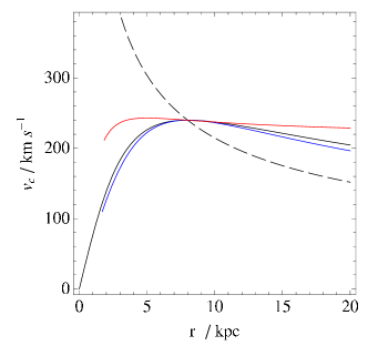
Figure 5.1: The in-plane rotation curves of the potentials specified in Table 5.1 and Table 5.5. Solid black line: the isochrone potential. Dashed black line: the Kepler potential. Red line: the Stäckel potential SP2. Blue line: the Stäckel potential SP1. Parameters in all potentials have been tuned to give a circular speed of $v_{c}=240\,{\rm km}\,{\rm s}^{-1}$ at the Solar radius $R_{0}=8\,{\rm kpc}$.

Figure 5.2: The real-space trajectories of the orbits (left-to-right, top-to-bottom) K1, I1, I2, I3, I4 and I5, as described in Table 5.2. The trajectories were evaluated in the Kepler potential (for K1) and the isochrone potential (for I1–I5) of Table 5.1.

5.3.2.1 Numerical tests

Table 5.1 describes a Kepler potential in which we will now confirm this prediction numerically. The parameter $M$ of this potential was chosen to reproduce a fiducial circular velocity $v_{c}=240\,{\rm km}\,{\rm s}^{-1}$ at the approximate solar radius of $R_{0}=8\,{\rm kpc}$. Fig. 5.1 shows the rotation curve in this potential, along with the rotation curves for other potentials in use in this chapter.

A cluster of 50 test particles was created, with a Gaussian distribution of particles in action-angle space, defined by $\sigma_{J}=1\,{\rm kpc}\,{\rm km}\,{\rm s}^{-1}$ and $\sigma_{\theta}=5\times 10^{-3}$ radians. This cluster was placed on the orbit K1, given in Table 5.2. in the aforementioned Kepler potential. The orbit has a pericentre radius of about $1.5\,{\rm kpc}$ and an apocentre of about $13\,{\rm kpc}$, and is illustrated in Fig. 5.2.

Table 5.2: Actions and apses for selected orbits in the spherical potentials used in this chapter. We generally choose $J_{\phi}=L$ so all orbits remain in the $(x,y)$ plane. The trajectories of these orbits are illustrated in Fig. 5.2

	$J_{r}/\,{\rm kpc}\,{\rm km}\,{\rm s}^{-1}$	$L/\,{\rm kpc}\,{\rm km}\,{\rm s}^{-1}$	$r_{p}/\,{\rm kpc}$	$r_{a}/\,{\rm kpc}$
K1	$780.$	$1016.$	$1.5$	$13$
I1	$313.$	$1693.$	$5$	$13$
I2	$0.$	$1920.$	$8$	$8$
I3	$207.$	$1920.$	$6$	$12.5$
I4	$571.7$	$2536.$	$11$	$20$
I5	$215.4$	$3127.$	$7$	$20$

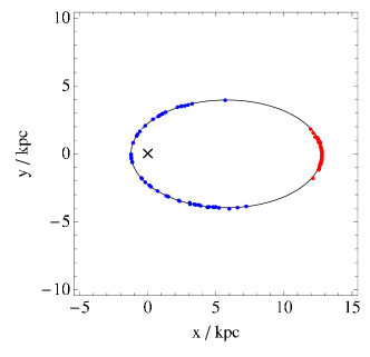
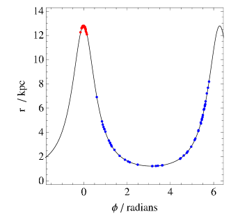
Figure 5.3: The solid line shows the orbit K1 (Table 5.2) in a Kepler potential (Table 5.1), on which a cluster of 50 test particles (initial conditions described in the text) has been evolved. The particles were released at apocentre. The red dots show the position of the test particles near apocentre, after 24 complete orbits, at $t=4.02\,{\rm Gyr}$. The blue dots show the same test particles near pericentre, approximately half an orbit later. In both cases, the dots delineate the underlying orbit precisely.

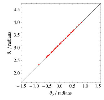
Figure 5.4: Angle-space configuration for the particles shown at apocentre in Fig. 5.3. The solid line shows the frequency vector ${\bf\Omega}_{0}$, with which the stream particles are perfectly aligned. There is also no secular spread in the direction perpendicular to the stream motion, as predicted in §5.3.2.

The cluster was released at apocentre, and evolved for $4.02\,{\rm Gyr}$, equal to 24 complete orbits, by integrating the equations of motion for each particle in the relevant potential. Fig. 5.3 shows the real-space configuration of the particles at the end of this time, and Fig. 5.4 shows the configuration of the same particles in angle-space.

The cluster has elongated to form a stream, that Fig. 5.3 shows to cover approximately half the orbit when the centroid is at pericentre. There is no spread in width in either real-space or angle-space. The stream delineates the cluster’s orbit in both figures perfectly. Fig. 5.3 shows that this is true irrespective of the real-space location of the centroid. Thus, the prediction of the previous section is validated.

5.3.3 Spherical harmonic oscillator

The spherical harmonic oscillator potential applies for motion within a sphere of uniform density (Binney & Tremaine, 2008, §3.1a), and is therefore of relevance to galaxy cores in the absence of a black hole. It has the form

$$\Phi(r)={1\over 2}\Omega^{2}r^{2}.$$ (5.37)

The Hamiltonian of the harmonic oscillator takes a particularly simple form

$$H(J_{r},L)=\Omega\left(L+2J_{r}\right),$$ (5.38)

where $\Omega$ is a constant. Comparing the above expression with equation (5.24), we see that like the Kepler Hamiltonian, the form of equation (5.38) admits the same stream geometry everywhere. In this case, however, the solutions to equation (5.28) are trivial, since ${\bf D}$ is a null matrix, and $\beta_{n}$ and $\lambda_{n}$ are identically zero for both $n=(1,2)$.

We conclude that clusters in harmonic potentials will always remain in the same configuration in angle-space, and will not spread out. Hence, streams cannot form in harmonic potentials. We further note that, in any case, it would be difficult to tidally strip a cluster in a harmonic potential, since the tidal force $dF_{\rm tide}$ across a cluster

$$dF_{\rm tide}\simeq{\partial^{2}\Phi\over\partial r^{2}}{\rm d}r=\Omega^{2}{\rm d}r,$$ (5.39)

is independent of galactocentric radius $r$. Thus, a cluster that is bound at apocentre in such a potential will remain bound elsewhere along its orbit.

5.3.4 Isochrone potential

The isochrone potential (Binney & Tremaine, 2008, §2.2.2d) is a simple potential which has several useful properties. It behaves as a harmonic oscillator in the limit of small radius, and as a Kepler potential at large radius, thus providing a reasonable model for a spherical galaxy across all radii. The form of the potential is

$$\Phi(r)={-GM\over b+\sqrt{b^{2}+r^{2}}},$$ (5.40)

where $b$ is a scaling constant, and the Hamiltonian is

$$H({\bf J})={-(GM)^{2}\over 2[J_{r}+{1\over 2}(L+\sqrt{L^{2}+4GMb})]^{2}}.$$ (5.41)

This Hamiltonian is not of the form of equation (5.24), and does not admit a globally applicable stream geometry. We therefore need to calculate the parameters (5.28) directly from $H$. We require the frequencies, which are obtained by direct differentiation

$$\Omega_{r} ={(GM)^{2}\over[J_{r}+{1\over 2}(L+\sqrt{L^{2}+4GMb})]^{3}},$$ (5.42)

$$\Omega_{\phi} ={1\over 2}\left(1+{L\over\sqrt{L^{2}+4GMb}}\right)\Omega_{r}.$$ (5.43)

We also require the derivatives of the frequencies with respect to the actions. We note that $\Omega_{r}$ can be written as a function of $H$ only,

$$\Omega_{r}={(-2H)^{3/2}\over GM},$$ (5.44)

and therefore its derivatives with respect to the actions are

$${\partial_{J_{r}}\Omega_{r}(H)} = \Omega^{\prime}_{r}(H)\,\Omega_{r},$$ (5.45)

$${\partial_{L}\Omega_{r}(H)} = \Omega^{\prime}_{r}(H)\,\Omega_{\theta},$$ (5.46)

where

$$\Omega^{\prime}_{r}(H)=-{3\sqrt{-2H}\over GM}.$$ (5.47)

We must calculate $\partial_{L}\Omega_{\phi}$ directly from equation (5.43). We find

$$\partial_{L}\Omega_{\phi}={2GMb\over\left(L^{2}+4GMb\right)^{3/2}}\Omega_{r}+{1\over 2}\left(1+{L\over\sqrt{L^{2}+4GMb}}\right)\partial_{L}\Omega_{r}.$$ (5.48)

From these expressions, we are now in a position to piece together values for the parameters (5.26), although the full expressions for $(\alpha,\beta,\gamma,\delta,\lambda)_{n}$ are not algebraically neat, and are therefore not very instructive. We do not repeat them here. We do note however that in the limit of $b\rightarrow\infty$ we recover the harmonic oscillator case of §5.3.3, and that in the limit of $b\rightarrow 0$ we recover the Kepler case of §5.3.2, as is required.

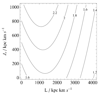
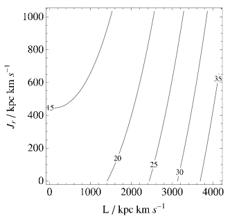
Figure 5.5: Details of stream geometry in the isochrone potential of Table 5.1. Left panel: the misalignment angle $\vartheta$, in degrees, between the principal direction of ${\bf D}$ and ${\bf\Omega}_{0}$, shown as a contour plot against the actions of the progenitor orbit. In all cases, $\vartheta$ is between $1.2^{\circ}$ and $2.2^{\circ}$ in angle-space. Right panel: The ratio of the eigenvalues $\lambda_{1}/\lambda_{2}$. The ratio is $>10$ everywhere and rises sharply with increasing $L$. The actions shown in both plots cover a range of interesting orbits, which are described in Table 5.3.

Table 5.3: The coordinate extrema of selected orbits from Fig. 5.5, illustrating the variety of orbits covered by that figure. The actions are expressed in $\,{\rm kpc}\,{\rm km}\,{\rm s}^{-1}$, while the apses are in  kpc.

$J_{r}$	$L$	$r_{p}$	$r_{a}$
$1000$	$4000$	$13$	$46$
$1000$	$\sim 0$	$\sim 0$	$12$
$0$	$4000$	$20.3$	$20.3$

In order to proceed, we must work with a specific example. Table 5.1 describes an isochrone potential, chosen to have the rotation curve maximized at $v_{c}=240\,{\rm km}\,{\rm s}^{-1}$ at the assumed solar radius of $R_{0}=8\,{\rm kpc}$. The rotation curve for this potential is plotted in Fig. 5.1.

What then is the geometry of streams formed in this potential? Fig. 5.5 shows the misalignment angle $\vartheta$, given by equation (5.31), and the ratio of the eigenvalues $\lambda_{1}/\lambda_{2}$, both as functions of ${\bf J}$. The range of ${\bf J}$ shown covers a variety of interesting orbits, described in Table 5.3.

The left panel shows that the principal direction of ${\bf D}$ is misaligned with the progenitor orbit for all values of ${\bf J}$, by $1$–$2^{\circ}$. The misalignment is at a minimum for both low energy and high energy circular orbits, and at a maximum for eccentric orbits with a guiding centre close to $r=b$. The right panel shows that the ratio of the eigenvalues $\lambda_{1}/\lambda_{2}$ varies from 15 to 25 across the range, with the ratio maximized for high energy circular orbits, and minimized for high energy plunging orbits.

Thus, we expect an isotropic cluster of test particles in this potential to form a stream in angle-space that is misaligned with ${\bf\Omega}_{0}$ by $1$–$2^{\circ}$ and is $15$–$20$ times longer than it is wide.

5.3.4.1 Numerical tests

We have created a cluster of 150 test particles, randomly sampled from a Gaussian distribution in action-angle space, defined by $\sigma_{J}=0.2\,{\rm kpc}\,{\rm km}\,{\rm s}^{-1}$ and $\sigma_{\theta}=10^{-3}$ radians. This cluster was placed on the orbit I1 from Table 5.2, which has an apocentre radius of $13\,{\rm kpc}$ and a pericentre radius of $\sim 5\,{\rm kpc}$, and is illustrated in Fig. 5.2.

The cluster was released at apocentre, and evolved for 94 complete azimuthal circulations, equal to a period of $t=22.75\,{\rm Gyr}$. Fig. 5.6 shows the angle-space configuration of the particles after this time. The arrowed, black line shows the orbit of the underlying cluster, ${\bf\Omega}_{0}$. The dashed line shows a straight line fit to the distribution of particles, which is clearly misaligned with the black line. We further note that, unlike the stream in the Kepler potential shown in Fig. 5.4, this stream is clearly also increasing in width.

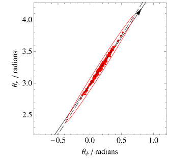
Figure 5.6: The angle-space distribution of a cluster of test particles, evolved on orbit I1 (Table 5.2) in the isochrone potential of Table 5.1 for 94 complete azimuthal circulations. The particles are shown at apocentre. The frequency vector ${\bf\Omega}_{0}$ of the progenitor orbit is shown with an arrowed black line. The stream is slightly misaligned with ${\bf\Omega}_{0}$; the dashed line is a straight line fit to the positions of the test particles, and clearly demonstrates this misalignment. Also plotted with a red solid line is the image in angle-space of a circle in action-space, mapped by ${\bf D}$. The shape and orientation of the image reflects the $\lambda_{n}$ and $\hat{{\bf e}}_{n}$ of ${\bf D}$ for this orbit. The ellipse is clearly misaligned with the underlying orbit, but is perfectly aligned with the stream particles.

We can predict the shape of this distribution precisely. Plotted as a red ellipse in Fig. 5.6 is the angle-space image of a circle in action-space, having been mapped by ${\bf D}$. After some time, the angle-space distribution of an isotropic cluster of test particles should take the form of a scaled version of this image. We see that the image and the particle distribution are indeed comparable, and that the dashed line is perfectly aligned with the principal axis of the image.

  

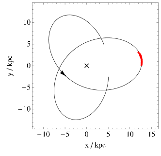
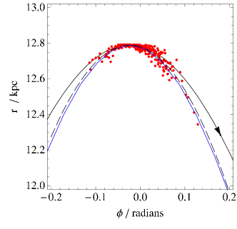
Figure 5.7: Real-space configuration for the stream of test particles shown in Fig. 5.6. The arrowed black line shows the trajectory of the progenitor orbit. The left panel shows an overview of the particles and the orbit; the cross marks the centre of the potential. The right panel shows a zoomed-in view of the particles, and is plotted in polar coordinates. The stream formed by the dots falls away in radius faster than does the orbit, in both forwards and backwards directions: the stream clearly does not follow the progenitor orbit. The dashed line is a quadratic curve least-squares fitted to the stream, which shows that the stream has a substantially greater curvature than does the underlying orbit. The solid blue line is the track predicted in §5.4.3 from the dashed line in Fig. 5.6: it agrees perfectly with the stream.

How does this misalignment manifest itself in real-space? Fig. 5.7 shows the real-space configuration of the cluster at the end of the simulation. The left panel shows an overview of the cluster in the orbital plane, while the right panel shows a close-up view of the cluster. The orbit of the cluster is drawn with a solid black line. In the right panel, the particles have been least-squares fitted to a quadratic curve, shown as a dashed line.

The progenitor orbit is clearly a poor representation of the stream. Although the orbit passes through the centroid of the stream, as expected, the curvature of the orbit is too low to match the stream adequately. Thus, the small misalignment in angle-space is manifest as a significant change in stream curvature at apocentre.

We conclude that, in this case, the track of the stream makes a poor proxy for the orbit of its stars, and that in general, streams cannot be relied upon to delineate orbits. In §5.5 we will highlight the errors that can be made in attempting to optimize potential parameters based on the assumption that they do delineate orbits. Firstly, however, we will discuss the details involved in the mapping of streams from action-angle space to real-space, in order that we may properly predict the track of a stream.

5.4 Mapping streams from action-angle space to real space

5.4.1 Non-isotropic clusters

Up until this point, we have considered our streams to form from a cluster of particles that is isotropic in ${\bf J}$, resulting in a stream that is perfectly aligned in angle-space with the principal direction of ${\bf D}$.

It is not obvious that this is a fair assumption. The structure in angle-space, given by equations (5.9) and (5.10), is linearly dependent upon the action-space distribution that generates it. By properly choosing that distribution, we can create streams of arbitrary shape in angle-space. Clearly, nature does not create clusters with arbitrary action-space distributions, so arbitrary-shaped streams do not emerge. But what kind of action-space distribution should be considered reasonable, that we may think of how it maps?

In §5.6 below, we will investigate the action-space distribution of real clusters, by means of N-body simulation. Here, we only require a qualitative understanding, in order to guess what kind of action-angle structures we should learn to map. Since the action-space distribution arises from the random motion of stars within the cluster, there is unlikely to be much complex structure. We will therefore assume that the distribution is ellipsoidal. But what should be the axis ratio of this ellipse?

Consider a cluster with isotropic velocity dispersion, $\sigma$, that is on an orbit with apocentre $r_{a}$ and pericentre $r_{p}$, where it is tidally disrupted. In our spherical system, the radial action is given by the closed integral

$$J_{r}={1\over 2\pi}\oint p_{r}\,dr,$$ (5.49)

where the integration path is one complete radial oscillation. Now consider a particle whose radial momentum $p_{r}$ differs from that of the cluster average by $\delta p_{r}\sim\sigma$. We can take a finite difference over equation (5.49) and thus obtain an expression for the the difference in radial action between the particle and the cluster

$$\delta J_{r}\sim{1\over\pi}\delta p_{r}\Delta r\sim\sigma\Delta r,$$ (5.50)

where $\Delta r=(r_{a}-r_{p})$ is the amplitude of the radial oscillation. Now consider another particle, whose azimuthal velocity differs from that of the cluster by $\delta v_{t}\sim\sigma$. The difference in angular momentum between this particle and the cluster is

$$\delta L\sim r_{p}\,\delta v_{t}\sim r_{p}\sigma,$$ (5.51)

where we have performed our calculation at pericentre, because that is where the cluster is stripped. For the purposes of this section, we are interested in the relative size of the spread in radial action $\Delta J_{r}$ and the spread in angular momentum $\Delta L$ for a disrupting cluster. We see that is approximately given by

$${\Delta J_{r}\over\Delta L}\sim{\Delta r\over\pi r_{p}}.$$ (5.52)

Although this ratio will take on every value between $(0,\infty)$ as we move from a circular orbit to a plunging one, for the orbits likely to be occupied by stream-forming clusters, it will typically be of order unity.

  

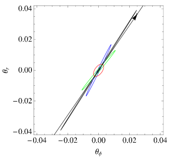
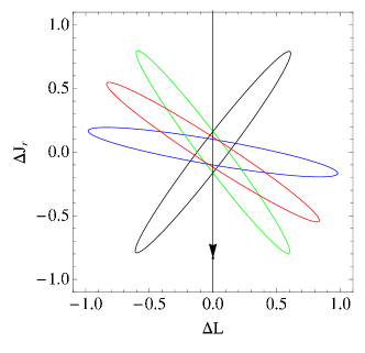
Figure 5.8: The right panel shows a selection of ellipses in action-space, each of axis ratio 10, but oriented in different directions. The left panel shows the image in angle-space that results from mapping each of the action-space ellipses with the Hessian ${\bf D}$, calculated for the orbit I1 in the isochrone potential of Table 5.1. In the left panel, the arrowed black line is the frequency vector ${\bf\Omega}_{0}$; in the right panel, the arrowed black line is the inverse map of the frequency vector, ${\bf D}^{-1}{\bf\Omega}_{0}$. We see that regardless of the shape in action-space, the mapped images are all elongated and roughly aligned with the orbit, although the alignment is generally not perfect. In this example, the misalignment of the red and green images is about $10^{\circ}$.

The right panel of Fig. 5.8 shows a set of ellipses, with axis ratio 10, placed at various orientations in action-space. The left panel of Fig. 5.8 shows the images of these ellipses in angle-space, following mapping by ${\bf D}$ when evaluated on I1. Note that all the images are both elongated and roughly oriented towards the principal direction. We conclude that the images of most action-space ellipses under this map—and thus, most streams formed in this potential—would be highly elongated and oriented to within a few degrees of the principal direction, which is itself oriented to within a few degrees of the frequency vector ${\bf\Omega}_{0}$.

Since the ratio of the eigenvalues for this orbit is $\sim 17$, it is not possible to produce an image in angle-space that is not elongated towards the principal direction, by mapping an action-space ellipse of axis-ratio 10. We note from Fig. 5.5 that, for this potential, the ratio of eigenvalues does not vary much, and nor does the principal direction stray from ${\bf\Omega}_{0}$ by more than a few degrees. We therefore conclude that reasonable action-space distributions will always result in the formation of streams in this potential, and that such streams will always be oriented in angle-space to within a few degrees of ${\bf\Omega}_{0}$.

5.4.2 The mapping of action-angle space to real space

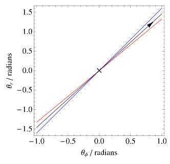
Figure 5.9: Three trajectories in angle-space. The black line is the trajectory of orbit I1, in the isochrone potential of Table 5.1. The red line has a frequency ratio $\Omega_{r}/\Omega_{\phi}$ that is $10\,\,\text{per cent}$ lower than I1. Conversely, the blue line has a frequency ratio that is $10\,\,\text{per cent}$ higher than I1. We note that the red line has retarded radial phase (relative to the black line) on the leading tail, and advanced radial phase on the trailing tail. Conversely, the blue line has advanced radial phase in the leading part, and retarded radial phase in the trailing part.

Fig. 5.9 shows three trajectories in angle space. The black line is the trajectory of I1 in the isochrone potential given in Table 5.1. The red line has a frequency ratio $\Omega_{r}/\Omega_{\phi}$ that is $10\,\,\text{per cent}$ lower than the black line, and is therefore rotated from it by approximately $2.9^{\circ}$. Conversely, the blue line has a frequency ratio that is $10\,\,\text{per cent}$ higher than the black line, and is therefore rotated from it by about $2.5^{\circ}$.

The red and blue lines were chosen to represent likely streams in angle-space that could form in the isochrone potential, given the results of the previous section. We note that the red line has retarded radial phase (relative to the black line) on the leading tail, and advanced radial phase on the trailing tail. Conversely, the blue line has advanced radial phase in the leading part, and retarded radial phase in the trailing part.

  

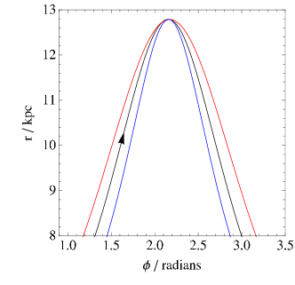
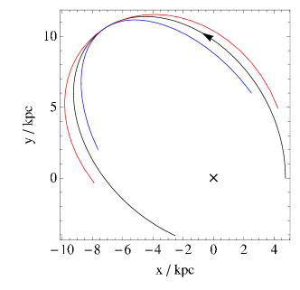
Figure 5.10: Plots of the real-space trajectories of the lines shown in Fig. 5.9, phase-matched near apocentre. Left panel: the trajectories plotted in polar coordinates. Right panel: the trajectories plotted in Cartesian coordinates; the centroid of the potential is marked with a cross.

How do these lines map into real-space? Fig. 5.10 shows the real-space curve obtained from the lines in Fig. 5.9, having chosen the point of intersection such that the lines are phase-matched near apocentre. The mapping is done by solving numerically for the real-space roots of the equations that relate action-angle variables to real-space coordinates: for spherical potentials, the appropriate equations are given in §3.5.2 of Binney & Tremaine (2008). The curves in Fig. 5.10 have been drawn by assuming that all points along each line have the same ${\bf J}$. Thus, this figure represents the real-space curves of streams oriented in angle-space according to Fig. 5.9, but formed from clusters of vanishingly small $\Delta{\bf J}$.

In Fig. 5.10 we see that the red line has systematically lower curvature than the black line. Conversely, the blue line has systematically greater curvature than the black line. We understand this, because the red curve has retarded radial phase on the leading tail, and advanced radial phase on the trailing tail, and thus is flattened with respect to the orbit. Similarly, the blue line has advanced radial phase on the leading tail, and retarded radial phase on the trailing tail, and thus appears curved with respect to the orbit.

  

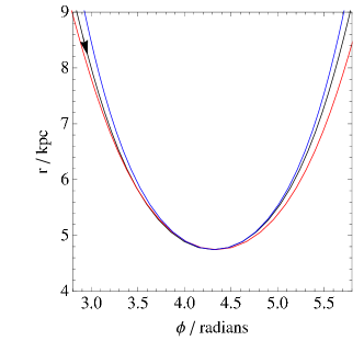
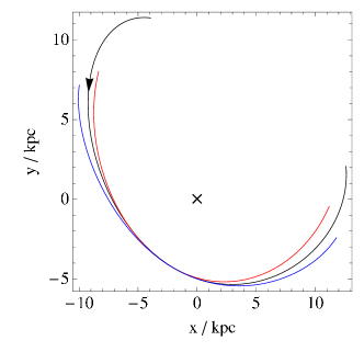
Figure 5.11: Similar to Fig. 5.10, but with the trajectories phase-matched near pericentre. The red line is again observed to have systematically lower curvature than the black line, and the blue line is again observed to have systematically greater curvature than the black line.

  

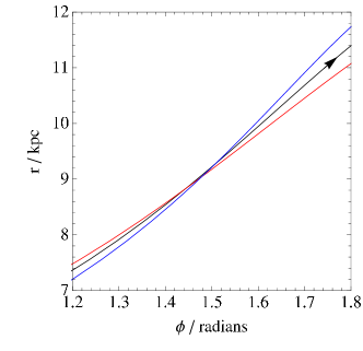
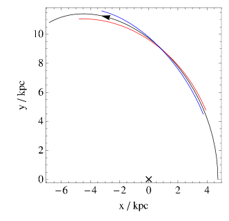
Figure 5.12: Similar to Fig. 5.10, but with the trajectories phase-matched at a point well away from apsis. In this case, a misalignment between the stream and ${\bf\Omega}_{0}$ in angle-space is expressed as a real-space misalignment, rather than a curvature error as at apsis. We note the similarity between the left panel and Fig. 5.9.

Fig. 5.11 shows the same lines, but now phase-matched at pericentre. Similarly to Fig. 5.10, the red line again appears flattened with respect to the orbit, and the blue line appears curved with respect to the orbit. Fig. 5.12 also shows the same lines phase-matched at a point well away from apsis. In this case, a misalignment between the stream and ${\bf\Omega}_{0}$ in angle-space is expressed as a real-space misalignment, rather than a curvature error as at apsis. We note the similarity between the left panel and Fig. 5.9 which occurs because, unlike at apsis, the mapping between angle-space and plane polar coordinates is relatively undistorted near this point.

5.4.3 Numerical tests

Figure 5.13: Real-space configuration of a 100 particle test stream, intended to check that our mapping of angle-space to real-space is accurate. The stream has an action-space distribution chosen to map under ${\bf D}$ to a line in angle-space oriented perpendicularly to ${\bf\Omega}_{0}$. The stream was released on orbit I1 in the isochrone potential of Table 5.1 and integrated for $23.6\,{\rm Gyr}$. The black curve is the orbit I1, while the red curve is the predicted stream track. The red curve is clearly a far better match to the particles than the black curve; the slight phase mismatch between the apocentre of the particles and the red curve is due to numerical error in the simulation process.

How can we be sure that our calculation of stream tracks from lines in angle-space is correct? We constructed a cluster of 100 test particles by randomly sampling a segment of a line in action-space, chosen such that its angle-space image would be a line oriented perpendicularly to ${\bf\Omega}_{0}$.

A point on the orbit I1 was chosen by integrating backwards $23.6\,{\rm Gyr}$ from apocentre. The cluster was placed at this point, released, and evolved forwards for $23.6\,{\rm Gyr}$. Fig. 5.13 shows the real-space configuration of the resulting stream at the end of this time. Also plotted are the orbit I1, as a black curve, and the stream track predicted from the line-segment in action space, as a red curve. The stream and the prediction are seen to agree almost perfectly.

We may further test our apparatus by predicting the track of the stream shown in Fig. 5.7. The blue line in the right panel of that figure shows the stream track predicted from a line in angle-space that is oriented precisely along the principal direction of ${\bf D}$ when evaluated for the orbit I1. The blue line is a much better match to both the stream data and the fitted line than is the orbit.

5.4.4 Are trajectories insensitive to small changes in ${\bf J}$?

So far, all the real-space tracks we have computed from streams in angle-space have assumed that the corresponding action for all points along that stream is that of the progenitor, ${\bf J}_{0}$.

This assumption is only strictly valid in the case of a vanishingly small action-space distribution, and for asymptotically large time since disruption of the cluster. If a mapping into real-space from a line in angle-space is made under this assumption, then a stream generated by a sufficiently broad action-space distribution will not be accurately represented, even though the representation in angle-space may be exact. This is because the small changes in action that give rise to the small changes in frequency also cause small changes in real-space trajectory as well.

When computing a stream track in real-space, it is possible to correct for this effect. By inverting equation (5.10) and eliminating $\Delta{\bf\Omega}$ using equation (5.9), we find that for a star separated from a fiducial point on the stream by angle $\delta\mbox{\boldmath$\theta$}$, the difference in action between the star and the fiducial point, $\delta{\bf J}$ is given by

$$\delta{\bf J}={1\over t_{d}}{\bf D}^{-1}\,\delta\mbox{\boldmath$\theta$},$$ (5.53)

where $t_{d}$ is the time since the star and the fiducial point were coincident. We may therefore guess the correction $\delta{\bf J}$ for a star’s true action $({\bf J}_{0}+\delta{\bf J})$ from its position in the stream, provided we know $t_{d}$.

We typically take the fiducial point to be the centroid of the stream, following which we may assume $t_{d}$ to be the time since the first pericentre passage of the cluster on its present orbit. Although this assumption neglects the possibility that the star could have been torn away during a subsequent pericentre passage, we note that during tidal disruption, it is the fastest moving stars which become unbound. The cluster core that remains after a pericentre passage therefore has lower velocity dispersion. Stars subsequently torn from that cluster will therefore have a smaller distribution in action-space. Consequently, the stars with the largest $\delta\mbox{\boldmath$\theta$}$ from the centroid—i.e. those for which the $\delta{\bf J}$ correction will be most important—must have been torn away at the earliest time, and so the assumption that $t_{d}$ equals the time since the first pericentre passage remains good.

But just how important is this effect? For small changes in $J_{r}$, the trajectory changes we discuss are expressed as changes in the radial amplitude $\Delta r$, while the guiding centre radius $r_{g}$, which is purely a function of $L$, is held constant. We can estimate the magnitude of the effect as follows.

Consider a cluster on an orbit close to circular, whose radial action is given by equation (5.49). Orbital energy $E$ is conserved, so close to apsis $r=r_{0}$, the radial momentum $p_{r}$ is given according to

$$E=p_{r}(r)^{2}+\Phi_{\rm eff}(r)=p_{r}(r)^{2}+\Phi_{\rm eff}(r_{0})+\left.{{\rm d}\Phi_{\rm eff}\over{\rm d}r}\right|_{r_{0}}(r-r_{0}),$$ (5.54)

where we have defined the effective potential $\Phi_{\rm eff}(r)=\Phi(r)+L^{2}/2r^{2}$. Since at apsis $p_{r}=0$, then

$$E=\Phi_{\rm eff}(r_{0}),$$ (5.55)

so from equation (5.54) we see

$$p_{r}(r)=\sqrt{-(r-r_{0})\left.{{\rm d}\Phi_{\rm eff}\over{\rm d}r}\right|_{r_{0}}}=\sqrt{(r-r_{0})F_{\rm eff}(r_{0})},$$ (5.56)

where we have defined the effective force, $F_{\rm eff}(r^{\prime})=-\partial\Phi_{\rm eff}/\partial r|_{r^{\prime}}$. If $(r_{a},r_{p})$ are apocentre and pericentre respectively, then we see that

$$p_{r}(r)\simeq\begin{cases}\sqrt{|F_{\text{eff}}(r_{a})|(r_{a}-r)}&\text{if }r\simeq r_{a},\\ \sqrt{|F_{\text{eff}}(r_{p})|(r-r_{p})}&\text{if }r\simeq r_{p}.\end{cases}$$ (5.57)

Hence, we might define the global approximation to $p_{r}$

$$\tilde{p_{r}}(r)={\sqrt{\left|F_{\rm eff}\right|(r-r_{p})(r_{a}-r)}\over\sqrt{r_{a}-r_{p}}},$$ (5.58)

with $F_{\rm eff}$ a constant set equal to the value of $F_{\rm eff}(r)$ taken at apsis, at both of which we assume it to take approximately the same value. We note that

$$\int_{r_{p}}^{r_{a}}\sqrt{(r-r_{p})(r_{a}-r)}\,{\rm d}r={\pi\over 8}\Delta r^{2},$$ (5.59)

so that when combined with equation (5.58), equation (5.49) becomes,

$$J_{r}={1\over 8}\sqrt{\left|F_{\rm eff}\right|\Delta r^{3}}.$$ (5.60)

We can deduce the value of $F_{\rm eff}$ as follows. We note that

$$\Phi_{\text{eff}}=\Phi+{L^{2}\over 2r^{2}},$$ (5.61)

and that its derivative is

$${{\rm d}\Phi_{\text{eff}}\over{\rm d}r}={{\rm d}\Phi\over{\rm d}r}-{L^{2}\over r^{3}}.$$ (5.62)

If the rotation curve is relatively flat, then $F_{\text{eff}}(r)$ evaluated at $r_{a}\simeq r_{g}+\Delta r/2$ is

$$F_{\text{eff}} =\left.{{\rm d}\Phi_{\text{eff}}\over{\rm d}r}\right|_{r_{a}}={v_{c}^{2}\over r}-{L^{2}\over(r_{g}+{1\over 2}\Delta r)^{3}}\simeq{v_{c}^{2}\over r_{g}}\left(1-{\Delta r\over r_{g}}\right)-{L^{2}\over r_{g}^{3}}\left(1-{3\over 2}{\Delta r\over r_{g}}\right)$$ (5.63)

$$=-\Delta r\left({v_{c}^{2}\over r_{g}^{2}}+{3L^{2}\over 2r_{g}^{4}}\right)=-{5v_{c}^{4}\Delta r\over 2L^{2}},$$ (5.64)

and similarly when evaluated at $r_{p}$, but with opposite sign. Equation (5.60) then becomes

$$J_{r}\simeq{1\over 8}\sqrt{5\over 2}{v_{c}^{2}\Delta r^{2}\over L}.$$ (5.65)

Differentiating the above expression, we find

$${{\rm d}J_{r}\over{\rm d}\Delta r} ={1\over 4}\sqrt{5\over 2}{v_{c}^{2}\Delta r\over L}$$ (5.66)

$$=\sqrt{{1\over 2}\sqrt{5\over 2}{J_{r}v_{c}^{3}\over L}}.$$ (5.67)

Hence, for a small change $\delta J_{r}$ we can estimate the corresponding change in the radial amplitude, $\delta\Delta r$, which is likely to be a good estimate for the positional error we would make in assuming that a star with action $J_{r}+\delta J_{r}$ actually had action $J_{r}$.

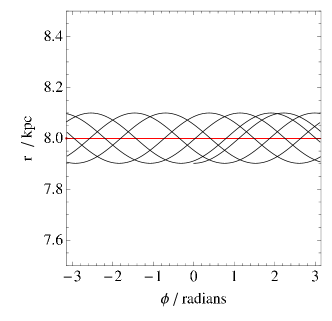
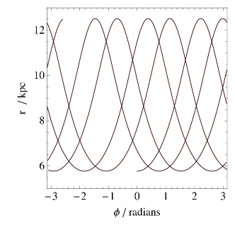
Figure 5.14: Plots to demonstrate the effect of changes in action $J_{r}$ on the real-space orbital trajectory of streams. The left panel shows that a small change in $J_{r}$ ($\delta J_{r}=0.21\,{\rm km}\,{\rm s}^{-1}\,{\rm kpc}$) to a circular orbit (I2 in Table 5.2) produces a change of $\delta\Delta r\sim 0.2\,{\rm kpc}$ in radial amplitude. The right panel shows the effect of the same perturbation $\delta J_{r}$ on an eccentric orbit (I3 in Table 5.2) with the same angular momentum as the circular orbit, but with $J_{r}=207\,{\rm km}\,{\rm s}^{-1}\,{\rm kpc}$. The effect on radial amplitude is so small as to be invisible in this plot.

We can confirm the predictions of the above equations numerically. The left panel of Fig. 5.14 shows the real-space trajectory of the circular orbit I2, with radius $r=8\,{\rm kpc}$, in the isochrone potential of Table 5.1. Also plotted is the trajectory of an orbit that has identical $L$ to I2, but $J_{r}=0.21\,{\rm km}\,{\rm s}^{-1}\,{\rm kpc}$.

Clearly, equation (5.67) ceases to have meaning when faced with orbits very close to circular, so we rely on the integral form given by equation (5.65) instead for our estimate. Equation (5.65) predicts $\Delta r=0.19\,{\rm kpc}$ for this perturbation from circular, which appears from the left panel of Fig. 5.14 to be close to exact.

From equation (5.67) we see that the magnitude of the effect diminishes as $\delta\Delta r\sim 1/\Delta r\sim 1/\sqrt{J_{r}}$. The right panel of Fig. 5.14 shows this to be the case. The panel shows two trajectories in the isochrone potential: one for the orbit I3, and one for the same orbit with $J_{r}$ incremented by $0.1\,\,\text{per cent}$. Equation (5.67) predicts a change $\delta\Delta R\sim 8\,{\rm pc}$. Close inspection of the trajectories confirms an actual $\delta\Delta r\sim 7\,{\rm pc}$, so the prediction is correct, but as is clear from Fig. 5.14, corrections of such magnitude are negligible.

What follows is an estimate for the positional error made by incorrectly guessing $L$. Consider again a cluster on an orbit close to circular. The angular momentum of the cluster is related to the guiding centre radius $r_{g}$ and the circular velocity $v_{c}$ by

$$L=v_{c}r_{g}.$$ (5.68)

Consider now a star whose angular momentum is suddenly reduced by $\delta L$. This star is now at apocentre, since its guiding centre radius has been reduced by

$$\delta r_{g}={\delta L\over v_{c}},$$ (5.69)

where we have assumed that the rotation curve is flat. Pericentre radius will have been reduced by of order twice the change in guiding centre radius, hence we may write

$$\delta\Delta r={2\delta L\over v_{c}}.$$ (5.70)

Thus, we can predict the change in radial amplitude $\delta\Delta r$ for a small change in angular momentum $\delta L$, which is likely to be a good estimate for the positional discrepancy we would encounter in assuming that a star with angular momentum $L+\delta L$ actually had angular momentum $L$.

Figure 5.15: Plot to demonstrate the effect of changes in angular momentum $L$ on real-space orbital trajectory. The trajectory of two orbits is plotted: the red line shows the trajectory of the orbit I2 (Table 5.2), while the black line shows the same orbit, except with $L$ incremented by $1\,\,\text{per cent}$.

Again, we can check the predictions of this expression numerically. Fig. 5.15 shows the trajectories of two orbits in our isochrone potential. The red line is orbit I2, while the black line is the same orbit, but with the angular momentum increased by $1\,\,\text{per cent}$. Equation (5.70) predicts $\Delta r\simeq 0.16\,{\rm kpc}$ for this change. Fig. 5.15 shows that this estimate is close to exact.

The only example we have shown thus far where this effect could be of consequence is the isochrone-potential stream shown in Fig. 5.7. For this cluster, equation (5.67) predicts that a positional error of $\sim 3\,{\rm pc}$ would be accrued by assuming all stars have the same radial action. Similarly, equation (5.70) predicts that a positional error of $\sim 1.5\,{\rm pc}$ will be accrued by assuming that all stars have the same angular momentum. These errors are insignificant, so no corrections are required in this case.

However, we shall see in some later examples that the errors will not be negligible. In these cases, the correction described by equation (5.53), properly accounting for variation in action down the stream, will be required. In such cases, we will assume that we accurately know $t_{d}$, the time since the first pericentre passage. In general we would not know $t_{d}$ accurately, although given ${\bf J}_{0}$ we could make a reasonable guess as to its value. However, even a poor, but finite, guess for the value of $t_{d}$ would likely produce a more accurate real-space stream track than would assuming ${\bf J}={\bf J}_{0}$ everywhere along the stream.

5.5 The consequences of fitting orbits

We confirmed in §5.3.4 that streams formed in the isochrone potential do not necessarily delineate orbits. In this section, we briefly examine the consequences should one attempt to constrain the parameters of the potential by assuming that these streams do delineate orbits.

We construct an experiment as follows. We first create three sets of pseudo-data, each containing a set of phase-space coordinates corresponding to one of the three stream tracks in Fig. 5.10. We choose to consider the streams from Fig. 5.10 because they are at apocentre, and many actual observed streams (e.g. the Orphan stream of Belokurov et al. (2007)) are discovered close to apocentre.

We now wish to measure the quality with which an orbit for a given set of isochrone potential parameters can be made to fit the data. Unlike in Chapters 2 and 3, where orbits were reconstructed from data for which only partial phase-space information is available, for this exercise we have granted ourselves pseudo-data with full and accurate positional and velocity information. This simplifies considerably the matter of finding an orbit that is close to the best fitting one.

We choose an orbit as follows. We first select a datum near the centroid of the stream, and declare that our chosen orbit must pass directly through this datum. Although it may be that some nearby orbit, one that does not pass directly through this point, would make a better-fitting orbit, any such orbit must pass very close to the selected datum, because it is close to the centroid. Thus, such an orbit cannot be much better-fitting than one that passes directly through the datum. Having chosen a datum, for a given set of potential parameters, an orbit is defined.

Having chosen our orbit, a goodness-of-fit statistic $\chi^{2}$ is calculated as follows. For each datum in the stream, with phase-space coordinate ${\bf w}_{i}$, a location along the orbit ${\bf w}^{\prime}_{i}$ is chosen that minimizes the square difference

$$({\bf w}_{i}-{\bf w}^{\prime}_{i})^{2}.$$ (5.71)

Having obtained the ${{\bf w}^{\prime}_{i}}$, the goodness-of-fit $\chi^{2}$ is defined by

$$\chi^{2}=\sum_{i,j}{(w_{i,j}-w^{\prime}_{i,j})^{2}\over\sigma^{2}_{j}},$$ (5.72)

where $j$ are the phase-space coordinates, and $\sigma_{j}$ is the rms of $(w_{i,j}+w^{\prime}_{i,j})/2$ over $i$. This $\chi^{2}$ statistic provides a dimensionless measure of the phase-space distance between the best-fitting orbit in a given potential, and the pseudo-data.

If the pseudo-data set were a sample of a perfect orbit in some potential, we expect the value of $\chi^{2}$ to be exactly zero, when the correct potential parameters are considered. As the potential parameters are varied away from their true values, we expect the value of $\chi^{2}$ to rise, as the best-fitting orbit becomes a steadily worse representation of the data. Hence, we expect minima in $\chi^{2}$ to be associated with the potential parameters that are optimum, from the perspective of fitting an orbit to the data. We seek such minima by plotting contours of $\chi^{2}$ over a range of likely values for the potential parameters.

5.5.1 Results

Three clusters of 50 test particles were created, with small initial angle-space distributions. The action-space distribution of each was a segment of a line, $\Delta J=0.2\,{\rm km}\,{\rm s}^{-1}\,{\rm kpc}$ long, and oriented such that, after a long time, the angle-space distribution of each would precisely match one of the three streams shown in Fig. 5.10.

Each cluster was placed on the orbit I1 in the isochrone potential of Table 5.1, and integrated forward for $77.04\,{\rm Gyr}$ to produce a thin stream about $10\,{\rm kpc}$ in length, that has its centroid at apocentre. The streams are then similar to those shown in Fig. 5.10. We declare each one of these streams to be a pseudo-data set for our experiment.

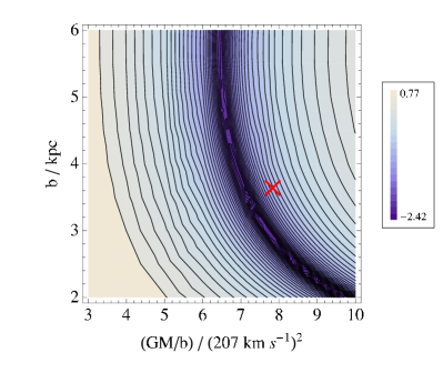
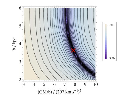
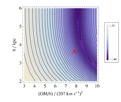
Figure 5.16: Plots of goodness-of-fit $\chi^{2}$ for the pseudo-data to the best-fitting orbit in the potential, for a range of potential parameters $(GM/b,b)$. The pseudo-data sets are 50 particle realisations of those streams shown in Fig. 5.10. Top panel: the red stream from Fig. 5.10; middle panel: the black stream from the same figure; bottom panel: the blue stream from the same figure. In each case, a valley of low values, corresponding to approximately degenerate solutions, can be seen. The red cross marks the correct parameters for the potential. In the case of the low-curvature stream of the top panel, the orbit fitting technique reports a lack of interior mass when compared with the middle panel. In the middle panel, the valley of solutions passes directly through the correct parameter coordinate, as expected. In the case of the high-curvature stream of the bottom panel, the orbit-fitting algorithm reports an excess of mass interior to the stream when compared with the middle panel.

Fig. 5.16 shows contours for the goodness-of-fit $\chi^{2}$, for the best-fitting orbit, in an isochrone potential with parameters $GM$ and $b$ as shown. In each case, a valley of low values, corresponding to a family of approximately degenerate solutions, can be seen. This degeneracy occurs because the trajectories (being at apocentre) are relatively insensitive to the shape of the rotation curve, but are very sensitive to the magnitude of the force. Hence, the family of solutions comprises those combinations of the $(GM,b)$ parameters that give rise to the same circular velocity at the radius of the stream. In each plot, a red cross marks the correct parameters for the potential.

In the case of the low-curvature stream of the top panel of Fig. 5.16, for all values of $b$, the orbit fitting technique reports a lack of interior mass when compared with the middle panel. In the middle panel, the valley of solutions passes directly through the correct parameter coordinate, as expected. Thus, the performance of the orbit fitting technique is validated. In the case of the high-curvature stream of the bottom panel, the orbit-fitting procedure reports an excess of mass interior to the stream for all values of $b$, when compared with the middle panel.

Thus, the attempt to constrain the potential parameters by using misaligned streams as proxies for orbits has led us to err. In the case of the low-curvature stream, for any given value of $b$, we have underestimated the mass by about $11\,\,\text{per cent}$. In the case of the high-curvature stream we have overestimated the mass by approximately $14\,\,\text{per cent}$.

We do note that the lowest value of $\chi^{2}$ seen for the two misaligned streams is significantly higher that the lowest value of $\chi^{2}$ seen for the perfectly aligned stream. This indicates that in the case of the misaligned streams, although optimum values for the parameters $(GM,b)$ are being found, the fit to the orbit is still not perfect there. This is precisely the effect utilized in Chapter 2 to try to identify the correct potential, and it is discussed there in further detail.

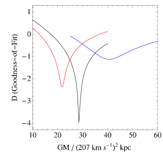
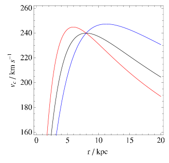
Figure 5.17: Left panel: goodness-of-fit $\chi^{2}$ for each pseudo-data set, to the best-fitting orbit in the potential. The colours of the curves for each pseudo-data set identify it with the corresponding stream from Fig. 5.10 from which it was derived. Right panel: rotation curves for the optimum potential found for each pseudo-data set. Unlike in Fig. 5.16, we have required that the circular velocity $v_{c}=240\,{\rm km}\,{\rm s}^{-1}$ at $R_{0}=8\,{\rm kpc}$. This reduces the potential to one of a single parameter; in this case, mass. The quality of the fits to the red and blue data sets is significantly degraded. Similarly to Fig. 5.16, utilizing the low-curvature, red data set as a proxy for an orbit causes us to underestimate the host mass by approximately 21  per cent. Utilizing the high-curvature, blue data set causes us to overestimate the host mass by approximately 54  per cent.

In the cases presented in Fig. 5.16, we have placed no constraints on the parameters of the potential other than those implied by the stream. This is a somewhat unrealistic test, since in practical usage one would generally require any acceptable potential to reproduce other observed features of the Milky Way galaxy, such as the circular velocity at the Solar radius. Most of the combinations of $(GM,b)$ in the family of solutions do not reproduce the correct circular velocity. We therefore repeat the test, while considering only those combinations of parameters that do.

Fig. 5.17 shows the value of $\chi^{2}$ obtained for the best fitting orbit, versus galaxy mass parameter $GM$, while requiring $b$ to take that value which gives the fiducial $v_{c}=240\,{\rm km}\,{\rm s}^{-1}$ at $R_{0}=8\,{\rm kpc}$. Like with Fig. 5.16, the quality of the fit at optimum $GM$ is significantly degraded for the misaligned streams when compared to the perfectly aligned stream. The correct value of $GM$ is obtained when fitting to the stream that perfectly delineates its orbit, thus validating the technique. However, the error in $GM$ when deduced using the low-curvature stream is $21\,\,\text{per cent}$, and the error in $GM$ when deduced using the high-curvature stream is $54\,\,\text{per cent}$. Hence, our attempt to use misaligned stream tracks to constrain the potential, while simultaneously requiring the potential to be consistent with other observations, has led us to yet greater error.

In conclusion, we find that there is a risk of substantial systematic errors in parameter estimation being made, if one attempts to constrain the potential using streams, and one assumes that streams perfectly delineate orbits.

5.6 The action-space distribution of disrupted clusters

Up until now, we have relied upon the qualitative estimate from §5.4.1 for what the action-space distribution of a disrupted cluster might be. In this section, we investigate the action-space distribution of various cluster models using N-body simulation. We further utilize our N-body models to confirm the misalignment between streams and orbits, and to demonstrate that we can accurately predict the real-space track of the stream.

The action-angle coordinates, as defined in the host galaxy potential, have limited usefulness when applied to the particles in a bound cluster, because the actions are not constant with time. Nonetheless, they remain a valid set of canonical coordinates and can be legitimately used to describe the phase-space distribution of the cluster. Moreover, we shall see that a disrupted cluster gives rise to a characteristic distribution in action-space, from which a precise track of the stream can be predicted.

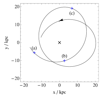
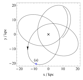
Figure 5.18: Plan views of the orbits used in this section. The left panel shows I4, with (a), (b) and (c) marking the positions of the cluster corresponding to the top-left, top-right and middle-left panels of Fig. 5.19 respectively. The right panel shows I5, with (a) marking the position of the cluster corresponding to the bottom-right panel of Fig. 5.23. In both panels, the potential in use was the isochrone potential described in Table 5.1.

Fig. 5.18 shows a segment of each of the orbits I4 and I5 in the isochrone potential of Table 5.1. These orbits were chosen to be fairly representative of those occupied by tidal streams in our Galaxy: they have apocentre radius $\sim 20\,{\rm kpc}$ and are moderately eccentric to allow for efficient tidal stripping. For our investigation, we wish to launch model clusters on each of these orbits, where the otherwise-stable cluster has been chosen such that its outermost stars will be torn away by tidal forces close to pericentre. The process by which we choose our model clusters is detailed in the next section.

5.6.1 Cluster models

We choose to work with King models (King, 1966; Binney & Tremaine, 2008) for our clusters, since these simple models are both easy to generate and are fairly representative of some observed globular cluster profiles (e.g. Fig. 6.18, Binney & Merrifield, 1998). The profile of a King model can be defined by $W\equiv\Phi_{0}/\sigma^{2}$, the ratio of the central potential to the squared-velocity parameter $\sigma^{2}$. The resulting family of models have similar profiles in terms of $\rho(\tilde{r}/\tilde{r}_{0})/\rho_{0}$, where $\rho_{0}$ is the central density and $\tilde{r}_{0}$ is the core radius. An exact model is specified by choosing $\rho_{0}$ and $\tilde{r}_{0}$, in addition to $W$, either directly or through a relation with another parameter.

For a given orbit, we specify our models as follows. Following the argument of Dehnen et al. (2004), we note that a cluster of mass $M_{c}$ orbiting at a galactocentric radius $r$ from the centre of a host galaxy with circular velocity $v_{c}$, will be tidally pruned to the cluster radius $\tilde{r}_{\text{tide}}$, where

$$\tilde{r}^{3}_{\text{tide}}\simeq{GM_{c}\over v_{c}^{2}}r^{2}.$$ (5.73)

We freely choose a profile parameter $W$ and a cluster mass $M_{c}$, and we also specify a galactocentric stripping radius $r_{s}>r_{p}$, where $r_{p}$ is the pericentre radius of the orbit concerned. We then set $\tilde{r}_{t}$, the cluster truncation radius, equal to $\tilde{r}_{\text{tide}}$ from equation (5.73), where $r\rightarrow r_{s}$ and $v_{c}\rightarrow v_{c}(r_{s})$. The resulting cluster will remain intact while $r\gg r_{s}$, but will have its outermost stars tidally stripped when $r\sim r_{p}$.

Table 5.4: Details of the cluster models used in this section. Defining parameters are in the central block of columns, while derived parameters occupy the right-hand block.

	$W$	$M_{c}$	$r_{s}$	$r^{\prime}_{\text{lim}}$	$\sigma$	$t_{\text{dyn}}$	$\epsilon$
C1	2	$10^{4}M_{\odot}$	$12\,{\rm kpc}$	$48.6\,{\rm pc}$	$1.18\,{\rm km}\,{\rm s}^{-1}$	$12.6\,{\rm Myr}$	$1.0\,{\rm pc}$
C2	2	$10^{5}M_{\odot}$	$12\,{\rm kpc}$	$104.8\,{\rm pc}$	$2.54\,{\rm km}\,{\rm s}^{-1}$	$12.6\,{\rm Myr}$	$2.2\,{\rm pc}$
C3	6	$10^{4}M_{\odot}$	$12\,{\rm kpc}$	$48.6\,{\rm pc}$	$1.14\,{\rm km}\,{\rm s}^{-1}$	$2.36\,{\rm Myr}$	$0.32\,{\rm pc}$
C4	2	$10^{4}M_{\odot}$	$11\,{\rm kpc}$	$45.5\,{\rm pc}$	$1.22\,{\rm km}\,{\rm s}^{-1}$	$11.79\,{\rm Myr}$	$0.94\,{\rm pc}$
C5	2	$10^{4}M_{\odot}$	$11\,{\rm kpc}$	$45.7\,{\rm pc}$	$1.22\,{\rm km}\,{\rm s}^{-1}$	$11.79\,{\rm Myr}$	$0.94\,{\rm pc}$
C6	2	$10^{4}M_{\odot}$	$15\,{\rm kpc}$	$56.3\,{\rm pc}$	$1.10\,{\rm km}\,{\rm s}^{-1}$	$15.6\,{\rm Myr}$	$1.2\,{\rm pc}$
C7	2	$10^{4}M_{\odot}$	$12\,{\rm kpc}$	$48.2\,{\rm pc}$	$1.19\,{\rm km}\,{\rm s}^{-1}$	$12.3\,{\rm Myr}$	$0.99\,{\rm pc}$

5.6.2 The disruption of a cluster

The low-mass cluster model C1 (Table 5.4) was specified for the orbit I4 (Table 5.2) according to the schema in §5.6.1. We chose a low value for the profile parameter of $W=2$ for our basic cluster model, in order to ensure the presence of many particles near the cluster truncation radius $\tilde{r}_{t}$ during successive stripping events.

A $10^{4}$ particle realization of the cluster model C1 was made by random sampling of the King model distribution function (Binney & Tremaine, 2008, equation 4.110). This cluster was placed at a point shortly after apocentre on the orbit I4 in the isochrone potential of Table 5.1. The cluster was evolved forward in time in the aforementioned potential by the fvfps tree code of Londrillo et al. (2003), using a time step of ${\rm d}t=t_{\text{dyn}}/100$ and a softening length $\epsilon$ as specified in Table 5.4. The simulated time period was $4.81\,{\rm Gyr}$, or almost 14 complete radial orbits.

Fig. 5.19 shows the evolution of the action-space distribution of the cluster model C1 as a function of time. In all the panels of that figure, an arrowed black line shows the mapping of the frequency vector from angle space into action space, ${\bf D}^{-1}{\bf\Omega}_{0}$. This vector shows the direction that maps onto ${\bf\Omega}_{0}$ in angle-space, so any action-space distribution that is aligned with this vector will be aligned with ${\bf\Omega}_{0}$ in angle-space.

In all cases involving the isochrone potential, ${\bf D}^{-1}{\bf\Omega}_{0}$ is oriented exactly along the $J_{r}$ axis. We can understand this from equation (5.43), which shows that in the isochrone potential, the frequency direction $\hat{{\bf\Omega}}_{0}$ is a function of $L$ only, and is independent of $J_{r}$. Thus, a line of constant $\hat{{\bf\Omega}}_{0}$ must map into action-space as a line of constant $L$. We note that this is a peculiar feature of the isochrone potential, and is not true for a general potential.

  

  

  

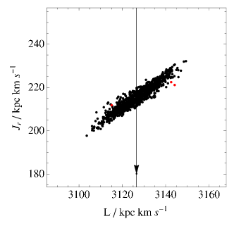
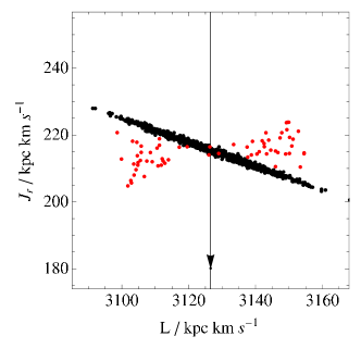
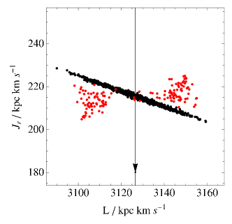
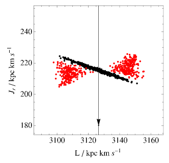
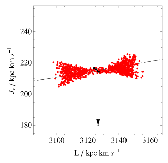
Figure 5.19: Plots showing the action-space distribution of particles for the N-body cluster model C1, at different times along the orbit I4. From left-to-right and top-to-bottom, these times are: shortly after release; first pericentre passage; first apocentre passage; second apocentre passage; 7th apocentre passage; 14th apocentre passage. The solid black line is the inverse map of the frequency vector, ${\bf D}^{-1}{\bf\Omega}_{0}$. The dashed line in the bottom-right panel represents a least-squares linear fit to the particle distribution.

The upper-left panel of Fig. 5.19 shows the configuration of the cluster immediately after release, at position (a) in Fig. 5.18. The distribution is ellipsoidal but without additional substructure, which we expect since the distribution in action results entirely from the approximately spheroidal density profile, and the approximately isotropic velocity dispersion, of the cluster. We understand the ellipticity of the action-space distribution from §5.4.1. Indeed, the prediction of equation (5.52) of $\Delta J_{r}/\Delta L\sim 0.3$ for this orbit can be seen to be approximately correct.

In the top-right panel of Fig. 5.19, the cluster has now moved from its point of release to its first pericentre passage, marked as position (b) in Fig. 5.18. We see that the ellipse has flattened somewhat, and has rotated anticlockwise. In the middle-left panel, the cluster has now progressed to the subsequent apocentre passage, marked as position (c) in Fig. 5.18. Here, the cluster is again flattened, but now it has rotated clockwise.

We can qualitatively understand this behaviour as follows. Consider a particle in a cluster near apsis. What changes to the actions will be made by perturbations to the velocity of this particle? A perturbation $\delta v$ to the transverse velocity will cause a change to the angular momentum

$$\delta L=r\delta v.$$ (5.74)

By means of the mechanism described by equation (5.70), this $\delta L$ will cause a change in the guiding centre radius $r_{g}$, which will cause a corresponding change in the radial action, according to equation (5.67). Conversely, a perturbation to the radial velocity will cause negligible change to the radial action, since

$$\delta E\simeq p_{r}\delta p_{r}=\dot{r}\delta v\sim 0,$$ (5.75)

and $J_{r}(E,L)$ remains unchanged. Hence, the distribution in both $J_{r}$ and $L$ is governed primarily by the transverse velocity, when the cluster is at apsis, and their highly correlated distribution reflects this.

  

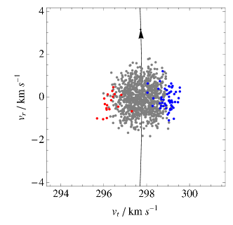
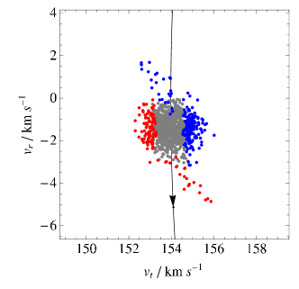
Figure 5.20: Plots of radial velocity against tangential velocity for the C1 cluster model, on the I4 orbit, at (left panel) the first pericentre passage, and (right panel) the first apocentre passage.

We can confirm this analysis by examining Fig. 5.20. The left panel shows $(v_{r},v_{t})$ for the cluster near its first pericentre passage, while the right panel shows the same for the cluster near its subsequent apocentre passage. The particles coloured red are those with $L<3110\,{\rm kpc}\,{\rm km}\,{\rm s}^{-1}$ and those coloured blue have $L>3140\,{\rm kpc}\,{\rm km}\,{\rm s}^{-1}$. The boundary between the colours is very sharp in the $v_{t}$ direction, as one would expect, since the particles have been coloured on the basis of $L$. However, we note that particles with the full range of $v_{r}$ contribute to both the blue and red regions equally, despite Fig. 5.19 showing that $J_{r}$ is very different for these two regions. Hence $J_{r}$ must be independent of $v_{r}$ near apsis.

We complete our explanation of the orientation of the action-space distribution by taking note of the sign of the change in $J_{r}$ near apsis. Increasing $L$ will always increase $r_{g}$, and when the cluster is at pericentre, this pushes $r_{g}$ further away, and so increases the radial action. Conversely, when the cluster is at apocentre, increasing $r_{g}$ brings it closer to the cluster, and so decreases the radial action. Thus, we see that near pericentre, particles with high $L$ will have high $J_{r}$ and the distribution will be rotated to have a positive gradient $\Delta J_{r}/\Delta L$. Conversely, at apocentre, particles with high $L$ will have low $J_{r}$, and so the distribution will be rotated to have a negative gradient $\Delta J_{r}/\Delta L$.

We can predict the value of the gradient of this distribution, by combining equation (5.67) and equation (5.70). We find

$${{\rm d}J_{r}\over dL}\sim\pm\sqrt[4]{10J^{2}_{r}\over L^{2}}\sim\pm\sqrt{\pi J_{r}\over L},$$ (5.76)

where the sign of the radical depends on the apsis under consideration, as detailed above. We can see from the upper-right panel of Fig. 5.19 that this equation predicts approximately the correct gradient, when evaluated for the orbit I4. Furthermore, we note that this equation implies that the gradient will be steeper for an orbit of greater eccentricity.

We now examine again Fig. 5.19, and note that the black particles are those still bound to the cluster, while the red particles are those that are unbound, where we have defined ‘bound’ to mean particles that are within $r_{\text{tide}}$ of the cluster barycentre. In the middle-left plot, which shows the cluster configuration at the first apocentre passage, the few unbound particles form an approximately horizontal distribution. These are particles that have been stripped from the cluster near pericentre, i.e. in the top-right panel of Fig. 5.19.

We note two things. Firstly, the bulk of the stripped particles have large $\Delta J$ from the cluster centroid; this is simply a consequence of the high-speed stars being most likely to be stripped. Secondly, we note that although the red particles in the middle-left panel span approximately the same range in $L$ as the black particles in the top-right panel, they span a range in $J_{r}$ that is only about half that spanned by the black particles.

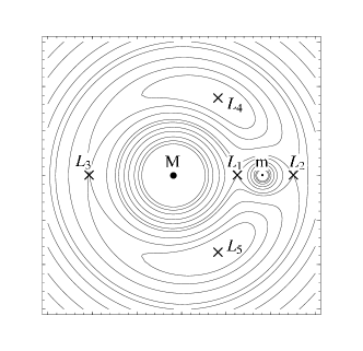
Figure 5.21: Lagrange points of neutral force, for the reduced three-body problem of a satellite of mass $m$ on a circular orbit around a host galaxy of mass $M>m$. The lines are contours of constant effective potential $\Phi_{\rm eff}$, as given for this problem by equation (8.87) of Binney & Tremaine (2008), who also provide a diagram similar to this. In the example shown, the frame rotates with the orbiting masses and the entire configuration is static with respect to time. In the case of a cluster on an eccentric orbit, the Lagrange points will not be static, but the points $L_{1}$ and $L_{2}$ through which cluster particles escape are always aligned radially with respect to the cluster and the host galaxy.

We explain this as a result of the cluster’s self-gravity, as follows. Particles that are stripped from the cluster mostly escape through the Lagrange points $L_{1}$ and $L_{2}$. As illustrated in Fig. 5.21, these two points are oriented along a radial that runs through the barycentres of the host galaxy and the cluster. Thus, it is the particles’ radial velocity which initially carries them away from the cluster, and it is from this velocity component that the particles pay most of the energetic penalty for escaping, with the consequence that the radial velocity dispersion of the escaping stars is reduced. This reduction in the radial velocity dispersion corresponds to a compression of the distribution in $J_{r}$ for escaping particles. Once unbound, the particles are carried further away from the cluster along a complex trajectory that ends up with the now-free particle drifting away from the cluster according to the mapping in equation (5.9). Thus, the final sum of the energetic penalty is paid from the difference in action ${\bf J}-{\bf J}_{0}$ between the particle and the cluster, with the net result that the unbound distribution uniformly shrinks. The latter effect is minor compared to the compression in $J_{r}$, because much more work is done in becoming unbound than in escaping to infinity once already unbound. Hence, the complete effect is to generate an unbound distribution, that looks like the high $\Delta{\bf J}$ wings of the pericentre distribution, but is compressed in $J_{r}$ and shrunk slightly.

Looking again at Fig. 5.19, we note that in the bottom-left panel, which corresponds to the 7th apocentre passage, many particles have now escaped, and the size of the bound distribution has visibly shrunk. We understand this as a consequence of the most energetic particles having already escaped the cluster, leaving behind a colder core. By the time of the 14th apocentre passage, shown in the bottom-right panel, almost all the particles have escaped. We note that the positions of many of the red particles have remained static between the bottom-left and bottom-right panels. The action-space distribution of the unbound particles is therefore frozen in place, confirming that self-gravity is unimportant in streams.

  

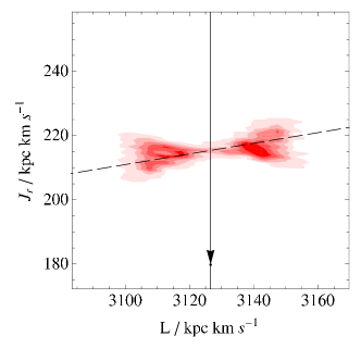
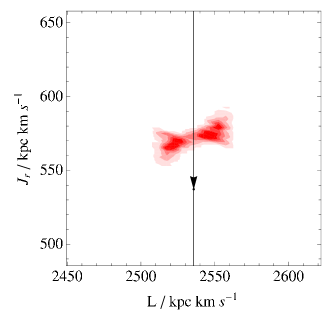
Figure 5.22: Plots showing the density of particles in action-space, corresponding to (left) the lower-right panel of Fig. 5.19, and (right) the lower-right panel of Fig. 5.23. The edges of the shaded areas represent contours of constant density, where the latter has been computed by placing particles into bins of width $\sim 2\,{\rm kpc}\,{\rm km}\,{\rm s}^{-1}$. Darker shading represents regions of higher particle density: the gross “bow-tie” structure is clearly seen, but no sub-structure is visible in either plot that is obviously unattributable to sampling noise.

The scatter plots in the bottom panels of Fig. 5.19 are filled too densely with particles to allow proper examination of the variation in particle density within the distribution. In order to elucidate this variation, the left panel of Fig. 5.22 shows a plot of particle density for the bottom-right panel of Fig. 5.19. The density field exhibits the same gross “bow-tie” structure that is visible in Fig. 5.19, and it further shows that particles are concentrated towards the centres of the lobes of the distribution, with particle density remaining low near the centroid. We explain this simply as a consequence of the number-density distribution of particles in velocity-space: the velocity-centroid of a cluster is populated with few particles because, although the phase-space density of particles there is high, the real-space volume associated with the lowest velocities is vanishingly small as one approaches the centroid, and so the velocity-space density is low there. This aside, no significant fluctuations in particle density can be seen in the left panel of Fig. 5.22 that are obviously unattributable to the effects of sampling noise.

In conclusion, we have qualitatively understood the distortion of a cluster in action-space as it passes through pericentre and apocentre along its orbit. We have found that stars stripped at pericentre form a distribution that is derived from the pericentre distribution of bound stars, but is compressed in $J_{r}$. We have found that the pericentre distribution will exhibit a high correlation between $J_{r}$ and $L$, and that the gradient of this correlation in $(L,J_{r})$ scales as $\sim\sqrt{J_{r}/L}$. We typically assume that our cluster orbit will have large $L$ and comparatively smaller $J_{r}$: this would only be untrue for extreme plunging orbits which are not likely to be relevant to the problem in hand. Hence the gradient in $(L,J_{r})$ will typically be less than unity, and the compression will only act to shrink it still further. Hence, the stripping mechanism always results in an action-space distribution that is both flattened and very roughly oriented along $\hat{L}$.

5.6.2.1 The effect of changing the cluster model or orbit

We now investigate the qualitative effects of changing the cluster model parameters, or the cluster orbit, on the action-space distribution of a disrupted cluster. The cluster models used in this section are C1 to C4, detailed in Table 5.4. These clusters were created according to the schema of §5.6.1, taking the orbit to be I4 in the isochrone potential of Table 5.1 for the models C1–C3, and taking the orbit to be I5 in the same potential for the model C4.

The cluster model C1, the evolution of which along the orbit I4 was detailed in the previous section, is used as our baseline to which we compare the distributions of the other clusters. The cluster model C2 has the same profile parameter, $W=2$, as does C1, but is 10 times more massive. The result is a cluster that is both heavier and proportionately larger while being stripped at the same galactocentric radius, $r_{s}$.

The cluster model C3 has the same mass as does C1, but is considerably more concentrated, with a profile parameter $W=6$. The cluster has an identical truncation radius $\tilde{r}_{t}$ and velocity scale $\sigma$, but has significantly fewer particles near to $\tilde{r}_{t}$, when compared with C1. The particles of C3 are generally more tightly bound to the cluster than are those of C1.

The cluster model C4 has the same mass and profile parameter as C1, but is specified for the orbit I5, which has lower $L$ than I4, and thus a smaller pericentre radius. The resulting cluster is slightly more compact, allowing it to survive to a closer galactocentric radius than can C1.

A $10^{4}$ particle realization of each of the models C1–C3 was placed at a point shortly after apocentre on the orbit I4, and evolved forward in time by the fvfps tree code, using a time step of ${\rm d}t=t_{\text{dyn}}/100$ and a softening length $\epsilon$ as specified in Table 5.4. The total period of the simulation was $2.36\,{\rm Gyr}$, or almost 7 complete radial orbits. Additionally, a $10^{4}$ particle realization of C4 was placed at a point shortly after apocentre on the orbit I5, and evolved forward in time by the fvfps tree code, for a total period of $2.21\,{\rm Gyr}$, or almost 7 complete radial orbits.

  

  

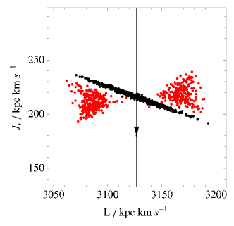
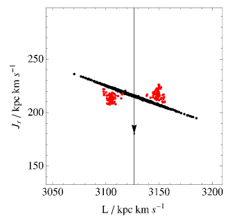
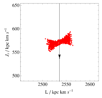
Figure 5.23: Plots showing the action-space distribution of particles for cluster models on various orbits. Each plot shows the distribution at the 7th apocentre passage. Black points are bound to the cluster, red points orbit free in the host potential. From left-to-right and top-to-bottom, the panels show: the C1 cluster on the orbit I4; the C2 cluster on the orbit I4; the C3 cluster on the orbit I4; and the C4 cluster on the orbit I5.

Fig. 5.23 shows the action-space distribution for the cluster at the seventh apocentre passage, for each of these simulations. The top-left panel shows C1 on the orbit I4, and is identical to the bottom-left panel in Fig. 5.19. The top-right panel shows the cluster C2 on the same orbit; the bottom-left panel shows the cluster C3 on the same orbit; and the bottom-right panel shows the cluster C1 on the orbit I5.

In the top-right panel, we see that the action-space distribution of the more massive cluster is qualitatively identical to that of C1, except that the distribution is approximately twice the scale. We conclude that cluster mass plays little role in determining the structure of the action-space distribution of disrupting clusters, but can determine the scale.

The bottom-left panel shows the distribution from the more centrally concentrated cluster C3. In this case, the shape of the distribution of unbound particles is approximately the same as for C1. However, the scale is much smaller: with more particles being near the core of the cluster, they have to work harder to escape, resulting in a colder action-space distribution. However, the distribution is still qualitatively similar to that of C1. Thus we conclude that cluster concentration can determine the scale of the action-space distribution, but not the general shape.

The bottom-right panel shows the distribution from the cluster C4 but on the orbit I5, which has the same apocentre radius as I4 but a pericentre radius about $33\,\,\text{per cent}$ smaller. Unlike in the other panels, the cluster has become completely unbound by the 7th apocentre passage on I5, which is likely to be a result of $(r_{s}-r_{p})$ being slightly larger for C4 on I5, when compared to the other clusters on I4, resulting in more efficient stripping at pericentre.

The distribution shown in this plot has approximately the same scale in $\Delta L$ as does the distribution from I4, but has approximately twice the scale in $\Delta J_{r}$. We can understand this, on account of the $\Delta J_{r}/\Delta L$ described by equation (5.76) being steeper for I5 than for I4. Further, since we have already noted that this cluster was stripped faster than was C1, the energetic penalty for escaping must be lower, and so we expect less compression in $J_{r}$. The resulting distribution is similar to that of the top-left panel, but less compressed in the $\hat{J_{r}}$ direction. Thus we conclude that changing the cluster orbit can distort the shape of the action-space distribution, but does not affect its basic structure.

The bottom-right panel is filled too densely with particles to gauge properly the density variation within it. We therefore provide a particle-density plot for the bottom-right panel, which is shown in the right panel of Fig. 5.22. This density plot correctly reproduces the gross structure observed in the scatter plot and reveals that the particles are concentrated in the lobes of the distribution, as was also true for the density plot in the left panel of Fig. 5.22. Aside from this, the plot reveals no further density fluctuations in the action-space distribution that cannot be attributed to sampling noise.

5.6.3 Predicting the stream from the action-space distribution

  

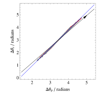
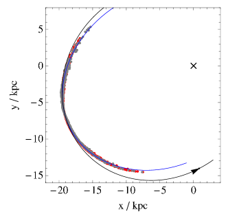
Figure 5.24: Plots of the distribution of particles for cluster C1, near its 14th apocentre passage on orbit I4. The left panel shows the angle-space distribution, while the right panel shows the configuration in real-space. The grey particles show positions directly computed from the N-body simulation, while the red particles show those positions predicted from mapping the action-space distribution in the bottom-right panel of Fig. 5.19. The two distributions almost precisely overlap. In both plots, the black arrowed curves show the trajectory of the progenitor orbit, while the blue curves show the mapping of the dashed line from Fig. 5.19. The blue curve is everywhere a much closer match to the stream particles than is the progenitor orbit.

We have determined the action-space distribution for several disrupted cluster models by means of N-body simulation. We now ask whether we can accurately predict the real-space path of the stream, given the action-space distribution of one of those models.

Suppose that we know the time $t_{p}$ since a cluster’s first pericentre passage. The angle-space distribution is predicted by equation (5.9), where ${\bf D}$ is evaluated on the progenitor orbit ${\bf J}_{0}$ and $t\rightarrow t_{p}$. We will use as an example the action-space distribution shown in the bottom-right panel of Fig. 5.19, which corresponds to the 14th pericentre passage of the simulated cluster C1 on the orbit I4. The left panel of Fig. 5.24 shows the angle-space configuration corresponding to this panel: the grey particles are for angles directly computed from the results of the N-body simulation, while the red particles are for those predicted by equation (5.9), assuming $t_{p}$ is known. Also plotted is the frequency vector ${\bf\Omega}_{0}$, shown as a black arrowed line. The distributions of black and grey particles in this panel agree perfectly. Furthermore, both distributions are obviously misaligned with the progenitor orbit.

The right panel of Fig. 5.24 shows the real-space configuration of particles for the same scenario. The grey particles are again plotted directly from the results of the N-body simulation, while the red particles result from the mapping into real-space of the red particles from the left panel. As in angle-space, the two distributions agree perfectly. Furthermore, the real-space manifestation of the misalignment of the stream with the orbit can be seen: the stream delineates a track that has substantially lower curvature than the orbit.

Our attempt to predict the real-space stream configuration from the action-space distribution has been completely successful. However, any complete model of the bottom-right panel of Fig. 5.19 must necessarily be rather complicated. It might not be possible to guess the form of this distribution without full N-body modelling. The dashed line in the bottom-right panel of Fig. 5.19 is a least-squares fit of the action-space distribution to a line. This represents a rather more simple model of the action-space distribution, which it might well be possible to guess ab initio for a cluster on a given orbit.

How good a prediction for the stream track can we get from this line? The blue lines in Fig. 5.24 show the results of mapping this line into both angle-space and then real-space. It is clearly an excellent fit to the stream, in marked contrast to the orbit, which represents a very poor model of the stream by comparison. Thus, even a very simple model of the cluster in action-space—albeit one deduced from an accurate knowledge of the distribution—allows us to predict stream tracks accurately.

Finally, we note that during the mapping of this line into real-space, we need to make a correction to the cluster’s action, as described by equation (5.53), to account for the variation in action down the stream. Evaluating equation (5.67) and equation (5.70) for the orbit I4, and taking ${\rm d}L\sim 25\,{\rm kpc}\,{\rm km}\,{\rm s}^{-1}$ and ${\rm d}J_{r}\sim 10\,{\rm kpc}\,{\rm km}\,{\rm s}^{-1}$ from the bottom-right panel of Fig. 5.19, we predict errors in the real-space of up to $\sim 0.2\,{\rm kpc}$ on account of the finite $L$ distribution, and up to $\sim 0.15\,{\rm kpc}$ on account of the finite $J_{r}$ distribution. These errors would be serious enough to be seen in Fig. 5.24, and thus the correction is required. We note, however, that even these substantial errors are insignificant compared to the several-$\,{\rm kpc}$ discrepancy between the stream and the orbit.

5.7 Non-spherical systems

We have investigated the formation of streams in spherical potentials, and demonstrated that they do not necessarily delineate streams, but that we can accurately predict their paths. Unfortunately, many real stellar systems in the Universe are not spherical. In particular, our own Galaxy, whose potential we are interested in probing with streams, is probably significantly flattened. In this section, we investigate the formation of streams in flattened potentials, and in particular we ask by how much they are misaligned with orbits. We also demonstrate that our apparatus is capable of correctly predicting stream tracks in flattened potentials, just as it is for spherical ones.

5.7.1 The general case with three actions

By analogy with §5.3.1, we now consider the case of a general axisymmetric stream-forming system, which is described by a Hamiltonian in three actions, $H(J_{1},J_{2},J_{3})$. Equation (5.16) can be written explicitly as

$$\Omega_{1}e_{n,1}+\Omega_{2}e_{n,2}+\Omega_{3}e_{n,3} =e_{n,1}\,\partial_{1}H+e_{n,2}\,\partial_{2}H+e_{n,3}\,\partial_{3}H$$

$$=\lambda(e_{n,1}\,\delta J_{1}+e_{n,2}\,\delta J_{2}+e_{n,3}\,\delta J_{3})+k_{n},\qquad(n=1,3).$$ (5.77)

Defining the constants $\alpha_{n}=e_{n,2}/e_{n,1}$, $\epsilon_{n}=e_{n,3}/e_{n,1}$, $\beta_{n}=k_{n}/e_{n,1}$ we have

$$\partial_{1}H+\alpha_{n}\partial_{2}H+\epsilon_{n}\,\partial_{3}H=\lambda_{n}(\delta J_{1}+\alpha_{n}\delta J_{2}+\epsilon_{n}\,\delta J_{3})+\beta_{n}.$$ (5.78)

As in the spherical case, we can find a general solution to the homogeneous form of this equation by considering an arbitrary function $f$ of the characteristic coordinates $\left(\delta J_{1}-{\delta J_{2}/\alpha_{n}}\right)$ and $\left(\delta J_{1}-{\delta J_{3}/\epsilon_{n}}\right)$. We add to this a particular solution for the inhomogeneous equation (5.78), to give the general solution

$$H=f\left(\delta J_{1}-{\delta J_{2}\over\alpha_{n}},\delta J_{1}-{\delta J_{3}\over\epsilon_{n}}\right)+\beta_{n}\delta J_{1}+{\lambda_{n}\over 2}\left(\delta J_{1}^{2}+\delta J_{2}^{2}+\delta J_{3}^{2}\right).$$ (5.79)

A system with a Hamiltonian of the form equation (5.79) is expected to exhibit globally consistent stream-forming geometry, described by the quantities $(\alpha,\beta,\lambda,\epsilon)_{n}$. Unfortunately, apart from trivial extensions of two-action systems such as the Kepler potential, there is no known Hamiltonian of the form equation (5.79) that is of relevance to galactic dynamics. Indeed, there is no known closed form for any non-trivial Hamiltonian in three actions that is relevant to galactic dynamics.

In principle, one would expand $f$ as a power series in its two variables, and relate the resulting coefficients to a Taylor expansion of the Hamiltonian, as was done for the two-action case in §5.3.1. However, in the absence of a suitable analytic case to study, we will proceed no further. In the remainder of the section, the values of $\beta_{n}$ and $\lambda_{n}$ will be computed directly from ${\bf D}$ by numerical means, which itself will be constructed numerically from non-algebraic expressions for the frequencies and their derivatives.

5.7.2 Stäckel potentials

The only known integrable systems of three actions are those described by Stäckel potentials (Binney & Tremaine, 2008, §3.5.3). An exhaustive treatment in the context of galaxy modelling is given in de Zeeuw (1985) and de Zeeuw et al. (1986).

Stäckel potentials are of particular interest to us because, in the appropriate coordinate system, the Hamilton-Jacobi equation is separable. Action-angle variables can therefore be defined for these systems in terms of integrals over a finite path. Paul Stäckel first showed that the appropriate coordinate system is that of confocal ellipsoidal coordinates, and that indeed this is the only coordinate system in which the Hamilton-Jacobi equation separates (de Zeeuw, 1985; Binney & Tremaine, 2008, p.228). It is in keeping with this that we note that Cartesian, spherical polar and cylindrical polar coordinates are themselves limiting cases of these coordinates.

We refer the reader to de Zeeuw (1985) for a detailed treatment of confocal ellipsoidal coordinates. We merely note here that we are adopting the de Zeeuw (1985) notation convention, and that we are restricting ourselves to considering only oblate axisymmetric potentials. In this case, the coordinate system becomes the prolate spheroidal coordinates $(\lambda,\phi,\nu)$, where $(\lambda,\nu)$ are the roots for $\tau$ of

$${R^{2}\over\tau+\alpha}+{z^{2}\over\tau+\gamma}=1,$$ (5.80)

where $(\alpha,\gamma)$ are scaling constants, and $q=\sqrt{\gamma/\alpha}$ is the potential shape parameter, and $(R,\phi,z)$ are the familiar cylindrical polar coordinates. The permitted range for $(\lambda,\nu)$ is given by the inequality

$$-\gamma\leq\nu\leq-\alpha\leq\lambda.$$ (5.81)

In the meridonal plane $(R,z)$, the coordinates $(\lambda,\nu)$ define a set of elliptic coordinates, while in the equatorial plane, $(\lambda,\phi)$ define a set of polar coordinates. A plot of the curves of constant $(\lambda,\nu)$ in the meridonal plane is shown in Figure 24 of de Zeeuw (1985). Of note is that curves of constant $\lambda$ are a family of confocal ellipses, and curves of constant $\nu$ are a family of confocal hyperbolas, and that everywhere the two sets of curves are orthogonal.

In limit of $\lambda\rightarrow-\alpha$, we note that the direction $\hat{\lambda}$ of increasing $\lambda$ is tangent with the radial vector $\hat{R}$ in cylindrical polar coordinates, while the direction $\hat{\nu}$ is tangent with the axial vector $\hat{z}$. We also note that in the limit of $\lambda\gg-\alpha$, the direction $\hat{\lambda}$ is tangent with the radial vector $\hat{r}$ in spherical polar coordinates, while the direction $\hat{\nu}$ is tangent with the polar vector $\hat{\theta}$.

The character of orbits in these potentials is as follows. The orbits circulate in $\phi$. The orbits nutate in $\lambda$ between two apses, where $-\alpha\leq\lambda_{\text{min}}\leq\lambda\leq\lambda_{\text{max}}$. The orbits bounce in $\nu$, with a floor of $\nu_{\text{min}}=-\gamma$ corresponding to $z=0$, and an apex of $\nu=\nu_{\text{max}}$ corresponding to $z=\pm z_{\text{max}}$. Consecutive excursions in $\nu$ take place sequentially above and then below the equatorial plane: this is a consequence of the degenerate ellipsoidal coordinate system.

The limit of $\lambda\gg-\alpha$ will almost always apply for the example orbits that we examine below. We can qualitatively understand the meanings of the actions $(J_{\lambda},J_{\phi},J_{\nu})$ in this limit as follows. $J_{\lambda}$ is a generalization of the radial action $J_{r}$ in spherical systems. Thus, an orbit with large $J_{\lambda}$ will be eccentric, while an orbit with null $J_{\lambda}$ will be confined to an ellipsoidal shell centred on the origin. An orbit with large $J_{\nu}$ will make excursions above and below the equatorial plane, while an orbit with null $J_{\nu}$ is confined to the equatorial plane. Since we are only considering axisymmetric potentials, then $J_{\phi}=L_{z}$, the $z$-component of angular momentum, always. Our procedure for calculating these actions, and their corresponding angles, from conventional phase-space coordinates is discussed further in §5.7.4 below.

Finally, we mention the form of the potential. In prolate ellipsoidal coordinates, an oblate axisymmetric Stäckel potential takes the form (de Zeeuw et al., 1986),

$$\Phi(\lambda,\nu)=-{(\lambda+\gamma)G(\lambda)-(\nu+\gamma)G(\nu)\over\lambda-\nu},$$ (5.82)

where de Zeeuw’s function $G(\tau)$ is determined once the density profile $\rho(z)$ along the $z$-axis has been chosen (see e.g. equation 23, de Zeeuw et al., 1986). Thus, the model is completely specified upon choosing $\rho(z)$ and the scaling parameters $(\alpha,\gamma)$.

5.7.3 Galaxy models with Stäckel potentials

de Zeeuw et al. (1986) shows that if one requires the density everywhere to be non-negative it is not possible to write down a Stäckel model in which the density $\rho(r)$ falls off with distance from he $z$-axis more rapidly than $r^{-4}$ as $r\rightarrow\infty$. This is because an elementary density on the $z$-axis $\rho(z)=\delta(z-z_{0})$ provides an off-axis density term that falls as $r^{-4}$. This behaviour rules out many classes of galaxy models, including disks with exponentially falling density profiles. However, we can construct models in which the density falls more slowly than $r^{-4}$ as $r\rightarrow\infty$. In particular, models with asymptotically flat rotation curves, i.e. those in which $\rho(r)\sim r^{-2}$, are allowed.

In the models used in this section, we specify the $z$-axis density profile

$$\rho_{z}(z)={-\gamma\rho_{0}\over(z^{2}-\gamma)}={-\gamma\rho_{0}\over\tau},$$ (5.83)

where we have made use of $z^{2}=\tau+\gamma$. In this case, de Zeeuw’s function $G(\tau)$ can be written in closed form (equation 49, de Zeeuw et al., 1986). Models specified by equation (5.83) become spherical at large radii and have a rotation curve that is asymptotically flat, with

$$\lim_{r\rightarrow\infty}v^{2}_{c}=-4\pi G\rho_{0}\gamma.$$ (5.84)

In the core of these models, the surfaces of constant density are approximately ellipsoidal, with axis ratio

$${a_{z}^{2}\over a_{R}^{2}}={2q^{2}\over(1-q^{2})^{2}}\left(1-q^{2}+q^{2}\log q^{2}\right),$$ (5.85)

where the central potential axis ratio $q=\sqrt{\gamma/\alpha}$. The models are completely specified by choosing a shape with $q$, a mass scale with $\rho_{0}$, and a distance scale with $\gamma$. The combination of an asymptotic logarithmic ‘halo’ and a flattened ‘disk’ in these models allow them to make a fair representation of the observed properties of disk galaxies, although the lack of freedom in the models severely restricts the shape of the flattened density profile that can be achieved.

Table 5.5: Parameters for the example Stäckel potentials used in this chapter.

	$\rho_{0}/10^{10}M_{\odot}/\,{\rm kpc}^{3}$	$-\alpha/\,{\rm kpc}^{2}$	$-\gamma/\,{\rm kpc}^{2}$
SP1	$0.361$	$29.64$	$8.89\times 10^{-3}$
SP2	$0.266$	$1.893$	$0.322$

Table 5.5 describes two such models. SP1 was chosen to simulate the highly flattened potential that may be felt in proximity to a heavy disk. The density axis ratio is fixed to be 10 near the solar radius of $R_{0}=8\,{\rm kpc}$, which is approximately the same ratio as for the (exponential) thin disk profile of the Milky Way (see Binney & Tremaine, 2008, Table 2.3). The specification is completed by requiring the rotation curve to peak at $R_{0}=8\,{\rm kpc}$ with a circular speed $v_{c}=240\,{\rm km}\,{\rm s}^{-1}$.

  

  

Figure 5.25: Stäckel models in use in this chapter. The left panels show the flattened model SP1, while the right panels show the rounder model SP2. The top panels show contours of $\log\rho/\rho_{0}$, while the bottom panels show contours of the potential $\Phi$.

We note that the asymptotic circular velocity in this model is $v_{c}=42\,{\rm km}\,{\rm s}^{-1}$, which can be regarded as the halo contribution to the circular speed. The model is too centrally concentrated, and the halo contribution is too weak, to realistically model the Milky Way. However, it is highly flattened, and so makes an interesting example in which to study stream geometry. The rotation curve for this model is plotted as the blue curve in Fig. 5.1, while contours of constant density and potential for this model are shown in the left panels of Fig. 5.25.

The SP2 model was chosen to provide a force field better matched to that of the Milky Way at those radii where streams are typically observed, while still being somewhat flattened near the plane. The model was required to have $v_{c}=240\,{\rm km}\,{\rm s}^{-1}$ at $R_{0}=8\,{\rm kpc}$, and $v_{c}\geq 235\,{\rm km}\,{\rm s}^{-1}$ at $R=20\,{\rm kpc}$. The rotation curve was also required to peak at a radius not larger than $R=5\,{\rm kpc}$. Finally, the model was required to be as flat as possible, subject to satisfying these constraints. These requirement completely specify the model, which has an asymptotic circular velocity of $v_{c}=215\,{\rm km}\,{\rm s}^{-1}$. The disk contribution to this model is therefore arguably rather weak, but it is in most respects a more reasonable model for the Milky Way galaxy than is SP1. The rotation curve for SP2 is plotted as the red curve in Fig. 5.1, while the right panels of Fig. 5.25 show contours of constant density and constant potential for this model.

5.7.4 Stream misalignment in Stäckel potentials

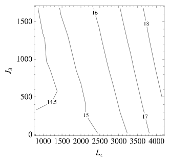
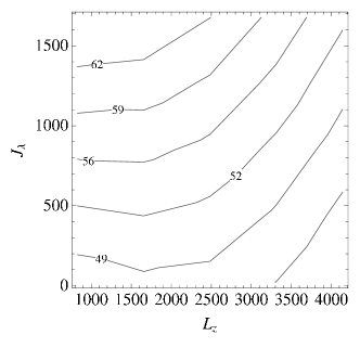
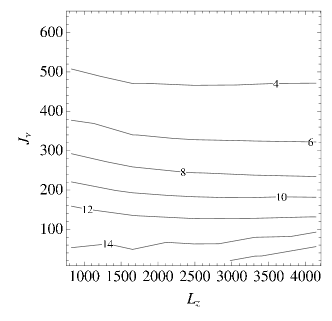
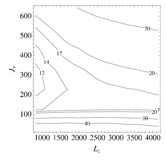
Figure 5.26: Details of stream geometry for the Stäckel potential SP1. Left panels: contours for the misalignment angle $\vartheta$, in degrees, between the principal eigenvector of ${\bf D}$ and ${\bf\Omega}_{0}$, shown as a function of ${\bf J}$. Right panels: contours for the eigenvalue ratio $\lambda_{1}/\lambda_{2}$. The top panels show the plane in action-space with $J_{\nu}=20.7\,{\rm kpc}\,{\rm km}\,{\rm s}^{-1}$, while the bottom panels show the plane in action-space with $L_{z}=414\,{\rm kpc}\,{\rm km}\,{\rm s}^{-1}$. The range of actions covers a variety of interesting orbits: details of orbits at the extremes of the range are given in Table 5.6

We now consider the geometry of streams formed in the Stäckel potentials SP1 and SP2. Although the form of the Stäckel potential allows the Hamilton-Jacobi equation to separate, and thus allows the actions ${\bf J}$ to be defined in terms of an integral over a single coordinate, expressions for ${\bf J}$ do not exist in closed form. Instead, the integrals in the expressions for ${\bf J}$ have to be evaluated numerically. Similarly, expressions for both the frequencies ${\bf\Omega}$ and their derivatives $\nabla_{\bf J}{\bf\Omega}$ can be written down, but not in closed form, and the integrals that they contain must too be evaluated numerically.

The details of the expressions for ${\bf J}$, ${\bf\Omega}$ and $\nabla_{\bf J}{\bf\Omega}$, and how to evaluate them, appear in Appendix A. Here, we simply note that having evaluated these quantities for a particular orbit, the eigenvectors $\hat{{\bf e}}_{n}$ and the eigenvalues $\lambda_{n}$ are computed directly from the matrix ${\bf D}({\bf J}_{0})=\left.\nabla_{\bf J}\Omega\right|_{{\bf J}_{0}}$ by standard methods.

Table 5.6: The coordinate extrema of selected orbits from Fig. 5.26, illustrating the variety of orbits covered by that figure. The actions are expressed in $\,{\rm kpc}\,{\rm km}\,{\rm s}^{-1}$, while the apses are in  kpc.

$J_{\lambda}$	$L_{z}$	$J_{\nu}$	$R_{p}$	$R_{a}$	$|z|_{\text{max}}$
$20$	$828$	$20$	$3.5$	$5$	$0.74$
$20$	$4140$	$20$	$20$	$26$	$2.5$
$1680$	$4140$	$20$	$14$	$70$	$7$
$1680$	$828$	$20$	$1.75$	$27$	$3$
$414$	$828$	$20$	$2$	$10$	$1.25$
$414$	$4140$	$20$	$16$	$38$	$3.5$
$414$	$4140$	$640$	$22$	$56$	$34$
$414$	$828$	$640$	$3$	$20$	$17$

We now examine the geometry of streams in the SP1 potential. The left panels of Fig. 5.26 show contour plots of the misalignment $\vartheta$ in angle-space between the principal direction of ${\bf D}$ and the frequency vector ${\bf\Omega}_{0}$, where $\vartheta$ is calculated from equation (5.31), as was the case for systems of two actions. The right panels of the same figure show contours of the ratio $\lambda_{1}/\lambda_{2}$. The range of actions shown in these plots covers a variety of interesting orbits; the apses of the orbits at the extremes of the range are described in Table 5.6

As with the equivalent plots for the isochrone potential (Fig. 5.5), we see that the principal direction of ${\bf D}$ is never perfectly aligned with ${\bf\Omega}_{0}$. We see that in this very flattened potential, those streams with low $J_{\nu}$ have the greatest degree of misalignment, at about $\sim 15^{\circ}$. These orbits spend much of their time near the disk, and never get very far from it. The misalignment diminishes with increasing $J_{\nu}$, falling to $\sim 4^{\circ}$ for orbits with apses in $z$ of some tens of  kpc. Hence, in this very flattened potential, there is much more prospect for dramatic misalignment than with the isochrone potential, which Fig. 5.5 shows to cause only comparatively smaller misalignments. Fig. 5.26 also shows that the eigenvalue ratio $\lambda_{1}/\lambda_{2}>10$ everywhere for the SP1 potential; thus, we conclude that highly elongated streams will form on all orbits which permit a cluster to be disrupted.

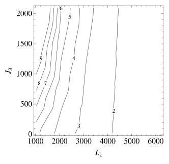
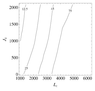
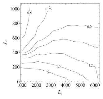
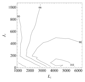
Figure 5.27: Similar to Fig. 5.26, but for the Stäckel potential SP2. The top panels show the plane in action-space with $J_{\nu}=20.7\,{\rm kpc}\,{\rm km}\,{\rm s}^{-1}$, while the bottom panels show the plane in action-space with $L_{z}=414\,{\rm kpc}\,{\rm km}\,{\rm s}^{-1}$. The range of actions covers a variety of interesting orbits: the behaviour of orbits at the extremes of the range is shown in Table 5.7

Fig. 5.27 shows the equivalent plot to Fig. 5.26, but for the SP2 potential. Like with the SP1 potential, the principal eigenvector is everywhere misaligned with ${\bf\Omega}_{0}$. The misalignment is maximized for plunging orbits, and minimized for highly inclined orbits. However, the magnitude of the misalignment is everywhere much smaller than is observed in the SP1 potential. For orbits that remain close to the plane, the magnitude of the misalignment is comparable to or larger than that seen in the isochrone potential (Fig. 5.5). For highly inclined orbits, the misalignment is slightly less than is seen in the isochrone potential, for orbits with similar apses.

Fig. 5.27 also shows that, like in the SP1 potential, the ratio of the eigenvalues of ${\bf D}$ is everywhere large. Hence, disrupted clusters should always form elongated streams in this potential.

Table 5.7: The coordinate extrema of selected orbits from Fig. 5.27, illustrating the variety of orbits covered by that figure. The actions are expressed in $\,{\rm kpc}\,{\rm km}\,{\rm s}^{-1}$, while the apses are in  kpc.

$J_{\lambda}$	$L_{z}$	$J_{\nu}$	$R_{p}$	$R_{a}$	$|z|_{\text{max}}$
$20$	$1030$	$20$	$3.5$	$5$	$1.5$
$2100$	$1030$	$20$	$2$	$30$	$7$
$20$	$6200$	$20$	$27$	$31$	$3$
$2100$	$6200$	$20$	$15$	$65$	$10$
$410$	$1030$	$20$	$2.5$	$10$	$5$
$410$	$6200$	$20$	$21$	$40$	$7$
$410$	$1030$	$1050$	$3$	$22$	$20$
$410$	$6200$	$1050$	$22$	$50$	$32$

In conclusion, we have found that in flattened Stäckel potentials with asymptotic logarithmic behaviour, streams will form from disrupted clusters on all realistic orbits, and that such streams will be generally misaligned with the orbits of the stars that compose them. If we take such potentials to be representative of the potential of our own Galaxy, we must conclude that, generally, streams observed in and around the Milky Way galaxy will not be perfectly aligned with orbits.

The precise behaviour of any given stream depends on both the potential and the action-space distribution of its stars. To proceed further we must again consider specific examples, by means of N-body simulation.

5.7.5 A stream in the Stäckel potential SP1

The top panels of Fig. 5.28 show the real-space trajectory of the orbit SO1 (Table 5.8) in the Stäckel potential SP1 (Table 5.5). This orbit has apses of approximately $R=(8,18)\,{\rm kpc}$ in the galactic plane, and $z=(-2,2)$ above and below the plane. It is thus fairly representative of an eccentric orbit that might be occupied by a globular cluster embedded in a galactic disk.

Figure 5.28: The real-space trajectories of the orbits SO1 (top panels), GD1 (middle panels) and OS1 (bottom panels), as described in Table 5.8. The trajectories shown were evaluated in the Stäckel potentials SP1 (for SO1) and SP2 (for GD1 and OS1), which are described in Table 5.5.

Table 5.8: Actions and apses for selected orbits in the Stäckel potentials used in this chapter. Since all examples are in axisymmetric potentials, $J_{\phi}=L_{z}$ generally. The trajectories of these orbits are illustrated in Fig. 5.28.

	$J_{\lambda}/\,{\rm kpc}\,{\rm km}\,{\rm s}^{-1}$	$L_{z}/\,{\rm kpc}\,{\rm km}\,{\rm s}^{-1}$	$J_{\nu}/\,{\rm kpc}\,{\rm km}\,{\rm s}^{-1}$	$R_{p}$	$R_{a}$	$|z|_{\text{max}}$
SO1	$252.3$	$2618.$	$20.5$	$8$	$18$	$2$
GD1	$143.4$	$2871.$	$357.3$	$10$	$19.5$	$12$
OS1	$1502.$	$2391.$	$533.4$	$6$	$37$	$26$

The cluster model C5 (Table 5.4) describes a King model specified for the orbit SO1 according to the schema of §5.6.1. The model has the same mass and profile parameter as does C1, and is very similar in all other attributes, because the orbit SO1 is not entirely dissimilar to the orbit I4 for which C1 was specified. A $10^{4}$ particle realization of the C5 was made by random sampling of the King model distribution function. This cluster was placed close to apocentre on the orbit SO1 and evolved forward in time by the fvfps tree code, with time step ${\rm d}t=t_{\text{dyn}}/100$ and softening parameter $\epsilon$ as specified in Table 5.4. The total period of the simulation was $2.15\,{\rm Gyr}$, or 7 complete radial oscillations.

5.7.5.1 Action-space distribution

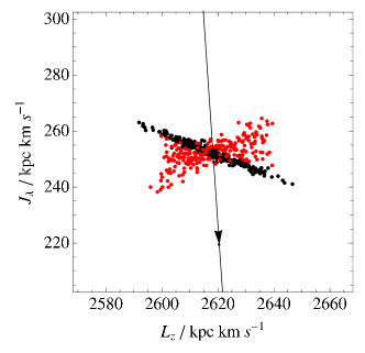
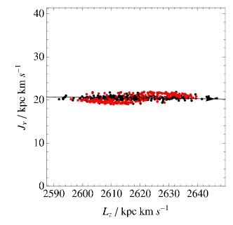
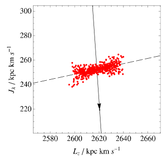
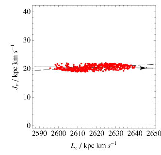
Figure 5.29: Action-space distribution for the simulated cluster C5, on the orbit SO1 in the Stäckel potential SP1, at various points in time. The left panels show the orthographic projection of distribution onto the $(L_{z},J_{\lambda})$ plane, while the right panels show a similar projection onto the $(L_{z},J_{\nu})$ plane. Distributions are shown at the following times: top panels, the first pericentre passage; middle panels, the subsequent apocentre passage; bottom panels, the 7th apocentre passage. Black particles are bound to the cluster, while red particles orbit free in the host potential. The dashed lines in the bottom panels are lines that have been least-squares fitted to the particles.

Fig. 5.29 shows the evolution of the action-space distribution of this simulated cluster with time. Each row of panels shows the distribution at a different point in time. The left panel in each row shows the orthographic projection of the actions onto the $(L_{z},J_{\lambda})$ plane, while the right panel of each row shows a similar projection onto the $(L_{z},J_{\nu})$ plane. In all panels, the appropriate projection of the mapped frequency vector, ${\bf D}^{-1}{\bf\Omega}_{0}$, is shown as an arrowed black line.

The top row shows the actions when the cluster is near to its first pericentre passage. In the left panel, the distribution is somewhat flattened, and oriented with positive gradient in $\Delta J_{\lambda}/\Delta L$. This behaviour is analogous with that seen in the top-right panel of Fig. 5.19: the motion of the cluster is predominantly in $(\lambda,\phi)$, thus $(J_{\lambda},L_{z})$ are good proxies for the radial action $J_{r}$ and angular momentum $L$ respectively. $J_{\lambda}$ and $L_{z}$ are therefore highly correlated for a cluster near apsis on this orbit, in analogy with the mechanism described by equation (5.76) in §5.6.2.

Conversely, the distribution in the right panel, while being narrow, is oriented almost exactly along $\hat{L}_{z}$. We can understand the shape as follows. For this orbit, which is confined to be close to the plane, $J_{\nu}\sim J_{z}/2$, where the factor of 2 appears because $J_{\nu}$ is defined on a path restricted to only one side of the plane. $J_{z}$ can be estimated by close analogy with equation (5.50). Hence, the spread in $J_{\nu}$ for a cluster of velocity dispersion $\sigma$ is approximately

$$\Delta J_{\nu}\simeq{1\over 2}\Delta J_{z}\sim{1\over 2\pi}\delta p_{z}\Delta z\simeq{1\over 2\pi}\sigma\Delta z.$$ (5.86)

By analogy with equation (5.52) we find

$${\Delta J_{\nu}\over\Delta L_{z}}\sim{\Delta z\over 2\pi R_{p}},$$ (5.87)

where $R_{p}$ is the galactocentric pericentre radius in cylindrical coordinates. Evaluating this expression for the orbit SO1 gives $\Delta J_{\nu}/\Delta L_{z}\sim 0.04$, which we see from the top-right panel of Fig. 5.29 is close to exact.

The flat orientation of the top-right panel we explain by pointing out that, as the top panels of Fig. 5.28 show, the motion in $\nu$ in this example is almost decoupled from the radial motion. This means that the $\nu$ coordinate need not be at apsis when the cluster is at pericentre, and thus the arguments of §5.6.2, which force a correlation between $J_{\lambda}\sim J_{r}$ and $L_{z}\sim L$ near pericentre, do not apply. For an orbit in which $J_{\nu}$ is more strongly coupled to the radial motion, we would expect to see the characteristic tilting of the $(L_{z},J_{\nu})$ distribution near pericentre and apocentre, as a correlation between $J_{\nu}$ and $L$ is forced.

The middle panels of Fig. 5.29 show the action-space distribution at the subsequent apocentre passage. Bound and unbound particles are shown in black and red, respectively. The action-space structure of the unbound particles in the left panel bears striking similarity to that shown in Fig. 5.19, as might be expected when $(J_{\lambda},L_{z})$ make good proxies for $(J_{r},L)$. The same physical principle for the disruption of the cluster applies here as it does in the spherical case; that is, the particles will escape the cluster through the Lagrange points $L_{1}$ and $L_{2}$ by first travelling radially, so the action-space distribution will be compressed in this direction. Thus, the range of $\Delta L_{z}$ and $\Delta J_{\nu}$ for the unbound stars is about the same as in the top panels, but the range of $\Delta J_{\lambda}$ is markedly less.

The bottom panels of Fig. 5.29 show action-space distribution at the 7th apocentre passage. The structure is essentially the same as that of the middle panels, except that all particles are now unbound. Also plotted in each of the bottom panels is a dashed line, which has been least-squares fitted to the unbound particles. We note that the image of the frequency vector and the dashed line are highly misaligned in the bottom-left plot; hence, we expect the stream to be significantly misaligned with ${\bf\Omega}_{0}$ in angle-space.

  

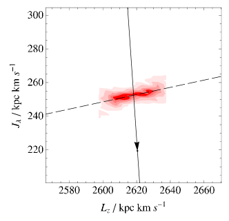
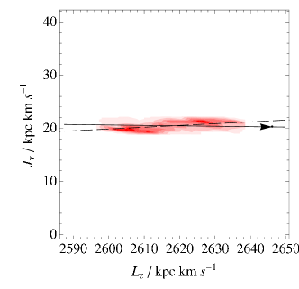
Figure 5.30: Plots showing the (column) density of particles in action-space, corresponding to (left) the bottom-left and (right) the bottom-right panels of Fig. 5.29. The density was estimated by placing particles into bins of width $\sim 2\,{\rm kpc}\,{\rm km}\,{\rm s}^{-1}$. Darker shading represents regions of higher particle density, with the edges of the shaded regions representing contours of constant density. As was true of Fig. 5.22, no significant sub-structure in the density field is visible that is not attributable to sampling noise.

In order to better examine the variation in particle density within the bottom panels of Fig. 5.29, Fig. 5.30 shows equivalent plots of particle density. As was seen in Fig. 5.22, the plots reveal the particles to be primarily concentrated in the lobes of the distribution, but they fail to reveal any significant additional structure in the particle-density field.

In conclusion, we find that in very flattened potentials, disrupted clusters form an action-space distribution that is wholly analogous with that found for disrupted clusters in spherical potentials. In the following section, we test the ability of a simple straight-line model of the action-space distribution to predict the track of the stream.

5.7.5.2 The effects of disk shocks

Unlike with a spherical potential, an axisymmetric potential allows for tidal forces other than those felt during pericentre passage to act upon an orbiting cluster. In particular, the passage of a cluster through a massive galactic disk will subject a cluster to a tidal force that is of comparable magnitude to that felt when close to pericentre.

The tidal stress imposed on a cluster at pericentre has a tensile component, which acts to strip stars from the cluster. Conversely, the tidal stress imposed by a disk passage is entirely compressive in nature. Hence, stars are not actively stripped from a cluster during a disk passage. Instead, the action of such ‘disk shocks’ is to heat the cluster, perhaps repopulating the outer edges of the cluster, the stars from which were stripped during a previous pericentre encounter (Spitzer, 1987, §5.2a).

The net effect of disk shocks on the stripping process is a faster and more complete disruption of the cluster than would take place for an unshocked cluster exposed to equivalent pericentric tidal stress. Since the vast majority of stars continue to be stripped at pericentre even when the effect of disk shocks is significant, the gross action-space distribution resulting from the stripping of a shocked cluster will remain as previously described. However, since the disk shocks act to increase the velocity dispersion of the cluster between stripping events, it is likely that the wings of the resulting action-space distribution will be populated with more stars than would otherwise have been the case.

5.7.5.3 Predicting the stream track

  

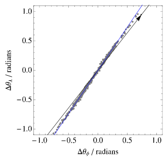
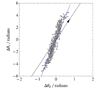
Figure 5.31: Angles for the N-body cluster shown in the bottom panels of Fig. 5.29. The blue line shows the predicted stream, resulting from the mapping of the dashed line in bottom panels of Fig. 5.29. The blue line is clearly a much better representation of the stream than is ${\bf\Omega}_{0}$, represented by an arrowed black line.

Fig. 5.31 shows the angle-space configuration for the simulated cluster near its 7th apocentre passage. The grey particles are for angles that have been computed directly from the output of the N-body simulation. The arrowed black line is ${\bf\Omega}_{0}$, while the blue line is the map of the dashed-line from Fig. 5.29. In both projections, the blue line is clearly a much superior match to the data than is the orbit.

  

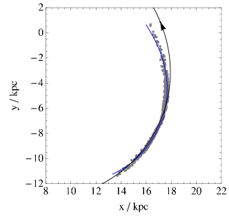
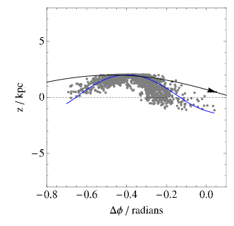
Figure 5.32: Real-space representation of an N-body simulation of cluster model C6 evolved on the orbit SO1. The potential is the flattened Stäckel potential of Table 5.1. The points are shown near the 7th apocentre passage following release. The black line shows the trajectory of an individual orbit; the blue line shows the predicted stream path.

Fig. 5.32 shows equivalent plot to Fig. 5.31, but in real-space. The misalignment between the stream and the progenitor orbit in angle-space is seen to map into a large misalignment in real-space. Attempting to constrain halo parameters by fitting orbits to the stream shown in Fig. 5.32 would not produce sensible results. Conversely, the map of the dashed-line model for the action-space distribution, shown in Fig. 5.29, clearly provides an excellent proxy for the track of the stream.

We therefore conclude that, in flattened systems, we are able to accurately predict the track a of stream using a simple, but well informed, action-space model, while the corresponding progenitor orbit makes a substantially less accurate proxy for the track of a stream.

5.7.6 Realistic examples in the Stäckel potential SP2

In this section, we draw on the work of the previous sections to construct N-body simulations for two actual observed Milky Way streams, in order to examine to what extent these streams can act as proxies for progenitor orbits.

In the following sections, we take as our model of the Milky Way the Stäckel potential SP2, described in Table 5.5. This model does reproduce an approximately correct in-plane rotation curve outside of the solar circle, precisely where our example streams reside. However, this model is arguably insufficient in representing the flattening of the potential in proximity to the Milky Way’s massive disk. §5.7.4 showed that stream misalignment is likely to worsen in the presence of a flatter potential. Thus, if our results below are in error, it is likely that streams make poorer proxies for orbits, not better ones.

Unfortunately, there is insufficient flexibility in Stäckel models to allow for an accurate representation of both halo and disk across a reasonable range of radii. Correcting for any error due to insufficient flattening, or even properly assessing the magnitude of its effects, is therefore beyond the scope of this chapter. It is with this caveat in mind that we now proceed.

5.7.6.1 Tidal stream GD-1

The tidal stream GD-1 (Grillmair & Dionatos, 2006) is associated with one of the most complete sets of full phase-space observations for any stream in the Milky Way, and has been utilized in several recent attempts (Willett et al., 2009; Koposov et al., 2010) to constrain the Galactic potential by fitting an orbit to it. Furthermore, it is the example used by this author (Chapter 4; Eyre, 2010) to demonstrate the applicability of Galactic parallax, the analysis of which would be subject to systematic error if the track of the stream were not tangent with the orbits of the stars. It is therefore of primary importance that we understand the behaviour of this particular stream.

The orbit GD1, described in Table 5.8 and illustrated in the middle panels of Fig. 5.28, was chosen to approximate the observed features of the GD-1 stream. In particular, the orbit was required to follow the conclusions of Chapter 4: i.e. it should be at pericentre, about $7\,{\rm kpc}$ distant from our fiducial Solar location; it should have an orbital plane inclined to the Galactic plane by $37^{\circ}$, and be on a retrograde orbit; and it should reproduce approximately the track on the sky as reported in Koposov et al. (2010).

Having selected an orbit in the SP2 potential that roughly meets these requirements, the cluster model C6 was specified according to the schema of §5.6.1. In the absence of any evidence as to the true nature of the GD-1 progenitor, the model was chosen to have the same mass and profile parameters as does C1. The stripping radius $r_{s}=15\,{\rm kpc}$ was chosen to be slightly larger than the pericentre radius of the GD1 orbit.

A $10^{4}$ particle realization of the C6 model was made by random sampling of the King model distribution function. This cluster was then placed close to apocentre on the orbit GD1, at a point $4.57\,{\rm Gyr}$ prior to the present pericentre location, equivalent to $14{1\over 2}$ radial orbits. The cluster was then evolved forward in time by the fvfps tree code, with time step ${\rm d}t=t_{\text{dyn}}/100$ and softening parameter $\epsilon$ as specified in Table 5.4.

  

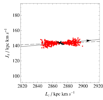
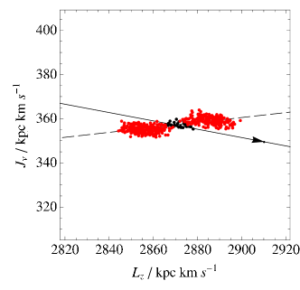
Figure 5.33: Actions for the cluster C6 on orbit GD1 in the Stäckel potential SP2. The result is intended to simulate a possible configuration of the GD-1 Milky Way stream. The cluster is shown near pericentre after $14{1\over 2}$ radial orbits. The arrowed black line is the image of the frequency vector, ${\bf D}^{-1}{\bf\Omega}_{0}$; the dashed line is a straight-line fit to the data.

  

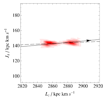
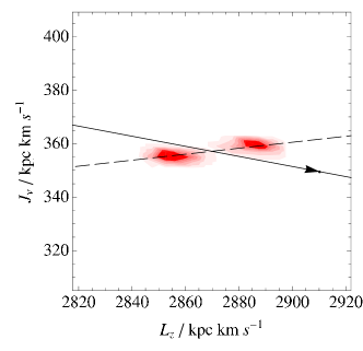
Figure 5.34: Plots showing the (column) density of particles in action-space, corresponding to the scatter plots of Fig. 5.33. The density was estimated by placing particles into bins of width $\sim 2\,{\rm kpc}\,{\rm km}\,{\rm s}^{-1}$. Darker shading represents regions of higher particle density, with the edges of the shaded regions representing contours of constant density.

Fig. 5.33 shows the action-space configuration of the simulated GD-1 cluster at the end of the simulation period, with the cluster centroid at pericentre, and the stream near its present location. Bound and unbound particles are plotted in black and red, respectively; we note that the cluster has been almost completely disrupted at this time. The image of the frequency vector, ${\bf D}^{-1}{\bf\Omega}_{0}$, is shown in this figure as an arrowed black line, while the dashed line is a least-squares fit to the unbound particles. In addition, Fig. 5.34 shows particle-density plots corresponding to the scatter plots of Fig. 5.33.

The action-space distribution does not look dissimilar to those in either Fig. 5.23 or Fig. 5.29. In this eccentric, highly inclined orbit, the ellipsoidal coordinates $(\lambda$,$\nu$) effectively parametrize the spherical polar coordinates $(r,\theta)$. The action $J_{\lambda}$ can therefore be compared to the radial action $J_{r}$, with $J_{\nu}$ becoming some function of the total angular momentum $L$ and $L_{z}$. In this example, $J_{\nu}$ is comparatively small, so $L\sim L_{z}$ and we can understand the left panel of Fig. 5.33 by direct analogy with the results of §5.6.2 and §5.7.5.1.

We will not attempt to disentangle the angular momentum $L$, in order to make sense of the right panel. Instead, we merely note that in comparison to the previous examples, the action-space image of the frequency vector ${\bf D}^{-1}{\bf\Omega}_{0}$ is aligned much more closely with the long axis of the action-space distribution. We therefore expect the misalignment between the angle-space stream and the frequency vector to be less here than in previous examples.

We can actually understand this alignment as a property of spherical, logarithmic potentials, which is approximately what this distant orbit feels in the Stäckel potential SP2. In such a potential, where

$$\Phi(r)=v_{c}^{2}\log{r/r_{0}},$$ (5.89)

the circular frequency $\Omega_{\phi}$ is given by

$$\Omega_{\phi}={v_{c}^{2}\over L}.$$ (5.90)

To first order, the radial frequency $\Omega_{r}$ is given by (Binney & Tremaine, 2008, §3.2.3)

$$\Omega^{2}_{r}=\left.{\partial^{2}\Phi_{\text{eff}}\over\partial r^{2}}\right|_{r_{g}}=\left.{\partial^{2}\Phi\over\partial r^{2}}\right|_{r_{g}}+{3L^{2}\over r_{g}^{4}}=-{v_{c}^{2}\over r^{2}_{g}}+{3v_{c}^{4}\over L^{2}}={2v_{c}^{4}\over L^{2}}=2\Omega^{2}_{L}.$$ (5.91)

Although the above equation is only true to first order—and indeed, it is the higher-order terms that contribute to ${\bf D}$ and give rise to the stream geometry seen in Fig. 5.27—we see that

$${\bf\Omega}_{0}=(\Omega_{r},\Omega_{\phi})\sim\Omega_{\phi}(\sqrt{2},1)\simeq{v_{c}^{2}\over L}(\sqrt{2},1).$$ (5.92)

The direction of ${\bf\Omega}_{0}$ is approximately constant, and the magnitude is a function of $L$ only. Hence, the image of $\hat{{\bf\Omega}}_{0}$ in action-space points almost exactly along $\hat{L}$.

We have seen from the arguments in §5.6.2 that the action-space distributions of clusters formed in spherical potentials are likely to be flattened and oriented towards $\hat{L}$. Thus, in spherical logarithmic potentials, we expect the long axis of such distributions to be aligned closely with the action-space image of the frequency vector. Correspondingly, we expect streams in such potentials to be more closely aligned with ${\bf\Omega}_{0}$ in angle-space than was seen in the isochrone potential or in the highly-flattened SP1 potential.

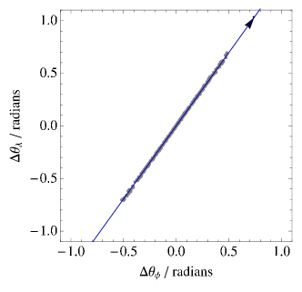
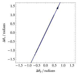
Figure 5.35: Angle-space configuration of the simulated GD-1 stream, shown in Fig. 5.33. The grey particles are computed directly from the results of the N-body simulation, while the blue line is the angle-space map of the dashed line from Fig. 5.33. The arrowed black like shows the frequency vector, ${\bf\Omega}_{0}$.

Returning to our example, Fig. 5.35 shows the angle-space configuration of the simulated GD-1 stream at the end of the simulation period. The grey particles are for angles that were computed directly from the output of the N-body simulation. The arrowed black line is ${\bf\Omega}_{0}$, while the blue line is the angle-space map of the dashed line from Fig. 5.33. As expected given the close alignment of the action-space distribution with the image of ${\bf\Omega}_{0}$, the stream, the frequency vector and the predicted track are all seen to agree almost perfectly.

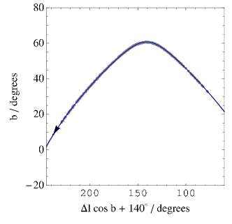
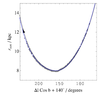
Figure 5.36: Real-space configuration of the simulated GD-1 stream, shown in Fig. 5.33. Plots are shown in Galactic latitude/longitude and heliocentric radius, to aid comparison with observations. Left panel: the on-sky projection of the stream, which is seen to agree perfectly with the progenitor orbit. Right panel: heliocentric distance, versus Galactic longitude. In the right panel there exists a tiny anomaly between the heliocentric distance of the stream and the trajectory of the orbit on the far left of the plot, but the agreement between stream and orbit is otherwise excellent.

Fig. 5.36 shows the real-space configuration of the simulated GD-1 stream and the end of the simulation period. The plots have been rendered in Galactic coordinates $(l,b)$ and heliocentric distance $r_{\rm sun}$ to aid with comparison to observations. The GD-1 stream is seen to be an excellent proxy for the progenitor orbit. This is expected, given the perfect alignment of the stream with ${\bf\Omega}_{0}$ in Fig. 5.35. A small discrepancy of $\sim 0.3\,{\rm kpc}$ does exist between the heliocentric distance of the stream and the orbit at the extreme end of the leading tail, but the match is otherwise perfect. In the case of the on-sky projection, the stream perfectly delineates the orbit for all longitudes. In both panels, the blue line, which is the track predicted from the dashed line in Fig. 5.33, is a perfect match to the stream everywhere.

In conclusion, we find that the simulated GD-1 stream delineates its orbit perfectly. This is fortunate for our analysis of the Galactic parallax of the GD-1 stream in Chapter 4, which does not now need to be revisited. We have understood the result in terms of a peculiar property of spherical logarithmic potentials, which causes the $\hat{L}$ direction in action-space to be mapped close to ${\bf\Omega}_{0}$ in angle-space. Since action-space distributions are naturally oriented close to $\hat{L}$, the result is an angle-space stream closely aligned with ${\bf\Omega}_{0}$.

5.7.6.2 Orphan stream

Our investigation into the utilization of tidal streams began with the Orphan stream (Belokurov et al., 2007), and the observation that standard techniques (e.g. Fellhauer et al., 2007b) had difficulty in finding an orbit that described it exactly. It is thus fitting that we end with the Orphan stream as our final case-study in this thesis.

The orbit OS1, described in Table 5.8 and illustrated in the bottom panels of Fig. 5.28, is based on the simulated Orphan stream shown in Chapter 2, which in turn is based on the tentative velocity data presented in Belokurov et al. (2007). The orbit OS1 roughly reproduces the on-sky track, distances, and velocities from Belokurov et al. (2007) when integrated in the SP2 potential. Recently, a newer analysis of the Orphan stream by Newberg et al. (2010) utilizing SEGUE spectra (Yanny et al., 2009) has produced radial velocity data that are considerably more certain, and unfortunately inconsistent with, the Belokurov et al. (2007) radial velocity data points. Nonetheless, we still present our simulation of the Orphan stream, in order to dispel any notion based on the previous section, that tidal streams in approximately spherical, logarithmic potential must always perfectly delineate orbits.

The cluster model C7 was specified according to the schema of §5.6.1, for the orbit OS1 in the SP2 potential. Like with GD-1, evidence as to the true properties of the Orphan stream progenitor is lacking. Hence, the model was chosen to have the same mass and profile parameters as does C1; the stripping radius $r_{s}=12\,{\rm kpc}$ was chosen to be slightly larger than the pericentre radius of the orbit.

A $10^{4}$ particle realization of the C7 model was made. This cluster was then placed close to apocentre on the orbit OS1, at a point $6.52\,{\rm Gyr}$ prior to the present apocentre location, equivalent to 14 complete radial orbits. The cluster was then evolved forward in time by the fvfps tree code, with time step ${\rm d}t=t_{\text{dyn}}/100$ and softening parameter $\epsilon$ as specified in Table 5.4.

  

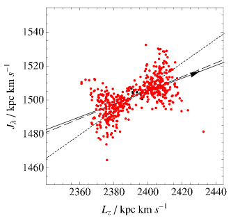
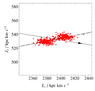
Figure 5.37: Actions for the N-body cluster C7 on orbit OS1 in the Stäckel potential SP2. The simulation is one possible configuration for the Orphan stream. The cluster is shown near apocentre after 14 complete radial orbits. The arrowed black line is the image of the frequency vector, ${\bf D}^{-1}{\bf\Omega}_{0}$. The dashed line is a least-squares fit to the data, and the dotted line is a weighted least-squares fit to the data, discussed in the text.

  

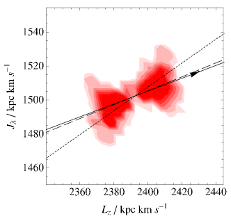
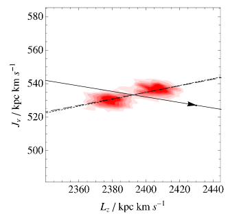
Figure 5.38: Plots showing the (column) density of particles in action-space, corresponding to the scatter plots of Fig. 5.37. The density was estimated by placing particles into bins of width $\sim 2\,{\rm kpc}\,{\rm km}\,{\rm s}^{-1}$. Darker shading represents regions of higher particle density, with the edges of the shaded regions representing contours of constant density.

Fig. 5.37 shows scatter plots for the action-space distribution of the model Orphan stream at the end of the simulated period, while Fig. 5.38 shows the corresponding particle-density plots. The distribution is immediately comparable to that of Fig. 5.33, except that the structure in the left panel appears tilted when compared to that of GD-1. We understand this to result from a combination of two factors. First, the orbit OS1 is more eccentric than is the orbit GD1. From equation (5.76) we expect this to result in a distribution that is steeper when viewed in $(L,J_{r})$. Secondly, unlike in the two previous examples, a large component of $L$ is in other than the $z$-direction. Hence, a distribution that is approximately aligned with $\hat{L}$ will not be aligned with $\hat{L}_{z}$. Again, we will not attempt to disentangle $L$ in order to precisely understand the mechanics of the plots, but we note once more that the image of the frequency vector ${\bf D}^{-1}{\bf\Omega}_{0}$ and the long axis of the action-space distribution are closely aligned. We thus expect the angle-space stream to be well represented by ${\bf\Omega}_{0}$.

Also shown in Fig. 5.37 are two least-squares fitted lines: the dashed curve is an unweighted fit to the particles, while the dotted line is a weighted fit to the particles, described in detail below.

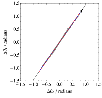
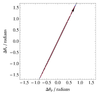
Figure 5.39: Angle-space configuration of the simulated Orphan stream, corresponding to the actions shown in Fig. 5.37. The angles of the grey particles have been computed directly from the N-body simulation. The arrowed black line is ${\bf\Omega}_{0}$, the blue line is the image of the dotted line from Fig. 5.37, and the red line is the image of the dashed line from Fig. 5.37.

Fig. 5.39 shows the angle-space configuration of the simulated Orphan stream at the end of the simulation run. The grey particles are for angles that were computed directly from the output of the N-body simulation. In both panels ${\bf\Omega}_{0}$, shown as a black arrowed line, is almost indistinguishable from the red and blue lines, which are the angle-space images of the dashed and dotted lines, respectively, from Fig. 5.37. All three lines almost perfectly delineate the stream, although close inspection shows the red line to pass on either side of the particles at the extremes of the tail, while ${\bf\Omega}_{0}$ and the blue line pass directly through.

Fig. 5.40 shows the real-space configuration of the simulated stream, at the end of the simulation run. The grey particles are plotted directly from the output of the simulation, while the lines are the real-space equivalents of those shown in Fig. 5.39.

  

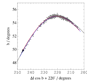
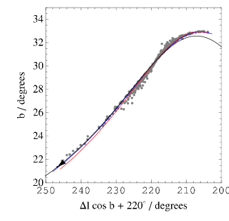
Figure 5.40: Real-space configuration of the simulated Orphan stream. The N-body particles are plotted in grey. The black line is the trajectory of the progenitor’s orbit, while the blue and red lines are the real-space mappings of the blue and red lines from Fig. 5.39. There is a clear anomaly between the orbit and the stream on the right-hand side of both plots. On the left-hand side of the right panel, there is an anomaly between the red curve and the stream.

We immediately note that the stream and the orbit trajectory do not coincide on the right side of each plot. Thus, the stream is not well represented by an orbit in this region, despite the stream and ${\bf\Omega}_{0}$ coinciding everywhere in Fig. 5.39. The explanation is that, although there is no misalignment between the stream and the orbit in angle-space, the changes in trajectory induced by the variation in action down the stream have caused the stream and the orbit to become misaligned in real-space. The detail of this mechanism was described in §5.4.4. In mapping from angle-space to real-space, the blue and red curves include the correction for this effect, as specified in equation (5.53). Thus, the predicted tracks from the red and blue curves match the stream much better than does the orbit, on the right-hand side of each plot, where the magnitude of this effect is maximized.

Looking again at Fig. 5.40 we see that on the left side of the right panel, the red curve is a slightly poorer representation of the stream than is the orbit or the blue curve. This occurs because the dashed-line model to the action-space distribution, shown in Fig. 5.37, is generating the wrong $\delta{\bf J}$ correction when utilized in equation (5.53). The wrong correction is generated because the stars at the ends of the tidal tails, rather than corresponding to the middling regions of the action-space distribution which are well modelled by the dashed line, actually correspond to the upper-right and lower-left extremities of the action-space distribution, which are well removed from the dashed-line model. Hence in this example, the dashed-line model does not provide an appropriate $\delta{\bf J}$ correction for the ends of the stream, and correspondingly the red line in Fig. 5.40 fails to properly predict the stream track at the end of the leading tail.

The remedy is a slightly more sophisticated model of the action-space distribution. The dotted line in Fig. 5.37 is a least-squares fit to the data, like the dashed line, but with each data point weighted by $\sigma_{i}={\bf D}\cdot\Delta{\bf J}_{i}$. That is, we grant greater weight to those data points which map to the fastest diverging stars in the stream. The resulting model, though still simple, better predicts the variation in action down the stream, when utilized in equation (5.53), than does the dashed line. The results of mapping the dotted line into real-space are shown as the blue line in Fig. 5.40. Unlike the red line or the orbit, the blue line matches the stream track everywhere.

In conclusion, we find that the action-space distribution of a simulated Orphan stream exhibits the same characteristics as those observed in both the isochrone potential, and for other orbits in Stäckel potentials. We find that, although the principal direction of ${\bf D}$ is misaligned with ${\bf\Omega}_{0}$, the stream in angle-space is nonetheless aligned with ${\bf\Omega}_{0}$, because it is a property of spherical, logarithmic potentials that the $\hat{L}$ axis in action-space maps to ${\bf\Omega}_{0}$ in angle-space, and it is a natural feature of disrupted clusters that their action-space distribution is also aligned with $\hat{L}$. Conversely, we find that the stream is not well represented by the progenitor orbit at all points in real-space, because the variation in action of the stars as we move down the stream causes sufficient change to the trajectory of those stars, that the stream track and the progenitor orbit diverge.

We find that we can predict the path of the stream perfectly, but that the simple model of a line least-squares fitted to the action-space distribution is not sufficient to do so. An improved model, in which the data points are weighted by the quantity ${\bf D}\cdot\Delta{\bf J}$ for the least-squares fit, results in an action-space model that accurately predicts the stream track everywhere.

5.8 Conclusions

In this chapter, we have studied in detail the mechanics of the disruption of star clusters in various model potentials. We have been interested in learning of the conditions required for the formation of tidal streams from such clusters, and in particular, to what extent such streams delineate the orbits of their stars. With regard to the latter, we have been motivated by the catalogue of techniques which attempt to utilize tidal streams to place constraints on the Galactic potential, many of which assume that streams perfectly delineate orbits.

We utilize action-angle variables extensively in our approach to the problem. It is found that these coordinates allow a convenient and natural description of the physical processes that occur in cluster disruption and stream formation. In the absence of more advanced techniques (e.g. McMillan & Binney, 2008), this approach has restricted the galaxy models under consideration to those for which action-angle variables are readily computed. Nonetheless, we do expect our findings to generalize to more sophisticated models of the Galactic potential.

In the broadest strokes, we have found that tidal streams will always form when a cluster in a realistic orbit around a realistic host galaxy is subject to tidal stripping. We show that these streams need not be well representative of an orbit in the host galaxy, and that in general they will not be, although clusters on particular orbits in particular potentials can well make an accurate representation. Particularly alarming is our finding that serious systematic errors can be made by attempting to constrain the Galactic potential using a stream that does not delineate an orbit. It is of some relief, however, that we find ourselves able to accurately predict the tracks of streams, even when they are not representative of an orbit, and so it may be possible to repair the potential-constraining procedures, by having them fit such stream tracks instead.

A complete summary of our findings in this chapter is presented below. The section that follows discusses some of the consequences of our findings, and presents some directions for future work. In Chapter 6 of this thesis we further review our findings in the context of contemporary Galactic astrophysics.

5.8.1 Summary

5.8.1.1 The physics of streams formation

In §5.2, we studied the formation of streams by considering the motion of small clusters of test particles, when described by action-angle coordinates of the host potential. We recalled from §8.3.1 of Binney & Tremaine (2008) that streams form in angle-space, when an initial, small structure in action-space results in a corresponding structure in frequency-space. This structure in frequency-space gives rise to a structure in angle space, which grows secularly and quickly dominates the original angle-space form of the cluster. Since the particles only feel the gravity of the host, the action-space structure remains frozen.

We show that the frequency-space structure is given by the transformation of the action-space structure under the linear map ${\bf D}=\nabla_{\bf J}H({\bf J})$, which is the Hessian of the Hamiltonian in the actions ${\bf J}$. This linear map can be characterized by the image produced from a unit sphere in action-space under its transformation. The sphere will be transformed into an ellipsoid, in which directions of the semi-axes correspond to the eigenvectors of the map, and the lengths of the semi-axes correspond to the eigenvalues of the map. Streams form when one of the eigenvalues of the map—and hence, the magnitude of the stretch in the principal direction—is very much larger than the other two.

5.8.1.2 Stream formation in systems of two actions

In §5.3 we investigate the form of this linear map for the general case of a system described by two actions. We find explicit relations between the geometry of the map and the form of the Hamiltonian, when written as a function of actions. We find that the Hamiltonians of the Kepler potential and of the spherical harmonic oscillator take a form in which the geometry of the linear map is globally consistent.

In the former case, one of the eigenvalues of the map is null, so the angle-space image of any action-space structure, under this map, will always be a perfect filament. We show that this filament will always be aligned precisely with the frequency vector of the progenitor orbit. Hence, disrupting clusters always form streams in the Kepler potential, and those streams always perfectly delineate the progenitor orbit. We go on to confirm this prediction numerically.

In the case of the spherical harmonic oscillator we show that the eigenvalues of the map are both null. Hence, the image of an action-space structure under this map is trivially null. The interpretation of this result is that streams cannot form in spherical harmonic oscillator potentials; all angle-space structure are perfectly preserved.

We also consider the case of the isochrone potential, for which the Kepler potential and the spherical harmonic oscillator are limiting cases. We find that in general the eigenvalues of the map are non-zero, but that the ratio between them is everywhere large. Hence, disrupting clusters will always form streams in this potential. Unlike with the Kepler potential, we find that the principal direction of the map is not generally aligned with the frequency vector of the progenitor orbit. Hence, the angle-space stream formed from a spherical cluster in action-space will also not be aligned with that frequency vector. We find that the misalignment in angle-space will typically be of order a few degrees. We go on to confirm this prediction numerically. We also show that this angle-space misalignment manifests itself in real-space as a failure of the progenitor orbit to delineate the track of the stream.

5.8.1.3 Considerations for the mapping of streams from action-angle space into real-space

In §5.4 we deduce general limits on the anisotropy of the action-space structure formed from a disrupting cluster. In doing so, we address the concern that a stream of arbitrary angle-space orientation could be created from a sufficiently non-isotropic action-space structure. We find that any realistic cluster, if it forms a stream at all, will form a stream that is not misaligned from the frequency vector, in angle space, by more than a few degrees.

We then take this result and examine the real-space tracks of lines in angle-space that are misaligned from the frequency vector by a few degrees. We find that the nature of the anomaly between the real-space track of such a line, and the orbit to which the frequency vector corresponds, depends on the phase of the orbit at which the observation is made. Specifically, we find that if the observation is made with the orbit close to apsis, then the angle-space misalignment manifests itself as a change in curvature of the stream track, with respect to the orbit. We find that if the observation is made at a point far from apsis, then the angle-space misalignment corresponds to a real-space misalignment, of similar magnitude.

The real-space position of a star is a function of both its action and its angle. Since it is a finite structure in action-space that gives rise to an angle-space stream, it follows that the action of the stars in a stream must vary down the track. In order to predict the real-space track of a stream, it is not then sufficient to know only the angle-space structure; one must also account for this variation in action along the angle-space stream. We investigate this variation, and deduce a method to detect when it will be of consequence for predicting the real-space track of the stream. We also show that the variation can be predicted, provided one can guess the time since the cluster’s first tidal stripping event, and provided one has an appropriate model of the action-space structure of the stream.

5.8.1.4 The consequences of fitting orbits using misaligned streams

In §5.5, we examine the consequences of attempting to utilize a misaligned stream to constrain the parameters of an isochrone potential, while assuming that the track does properly delineate an orbit.

When the stream perfectly delineates its progenitor orbit, we find that the potential parameters are isolated perfectly. Thus, we demonstrate the efficacy of our optimization technique. When the real-space curvature of the stream track is less than that of the progenitor orbit, we find that the mass parameter of the potential is consistently under-reported, by 11  per cent in our example case. When the curvature of the stream track is greater than that of the progenitor orbit, we find that the mass parameter is consistently over-reported, by 14  per cent in our example case.

However, in deducing these results, we have allowed ourselves to consider unrealistic combinations of parameters, which would be ruled out by independent observations. We therefore repeat the exercise, but we now consider only that family of potential parameters which correctly reproduces a fiducial circular velocity at the Solar radius.

When the stream perfectly delineates the progenitor orbit, we again find that the potential parameters are correctly identified. However, when the stream track has less curvature than the orbit, the best-fitting potential has a mass that is 21  per cent smaller than the truth. When the stream track has greater curvature than the orbit, the best-fitting potential has a mass parameter that is 54  per cent larger than the truth. Hence, adding extra constraints to the fitting process has resulted in the systematic errors becoming worse.

In summary, we find that large systematic errors can be made when attempting to optimize potential parameter by assuming that streams act as proxies for orbits, when they do not.

5.8.1.5 The action-space distribution of N-body clusters

In §5.6 we utilized N-body simulation of King model clusters to examine the action-space distribution resulting from the disruption of a live cluster.

We found that the action-space distribution of a disrupted cluster takes a characteristic shape, which is flattened, and is oriented with a small positive gradient when viewed in in the $(L,J_{r})$ plane. We find that the greater the eccentricity of the cluster orbit, the larger this positive gradient will be, but that in general, the distribution will be roughly oriented in the $\hat{L}$ direction in action-space. We are able to explain all features of this distribution in terms of the basic physical processes that apply to clusters undergoing tidal disruption. Hence, we predict that the action-space distribution of all disrupting clusters will take the same basic form, although details such as the density of stars across the distribution, and their precise dimensions and orientation, necessarily depend on the details of the model, the orbit, and the potential in question.

We show by simulation that real disrupted clusters do indeed form streams with tracks that are poorly predicted by the progenitor orbit. However, we show that by utilizing a simple, straight-line model of the action-space distribution, we are able to predict the real-space stream track of a stream with perfect accuracy.

5.8.1.6 Non-spherical systems

In §5.7, we extend the results of the previous sections to systems with a Hamiltonian described by three actions, allowing us to consider the stream-forming properties of non-spherical systems. As our example, we utilize oblate, axisymmetric Stäckel models with asymptotically logarithmic density profiles (de Zeeuw et al., 1986). We consider two such models: one highly flattened, and therefore representative of a heavy galactic disk; and one that is only slightly flattened, but is roughly consistent with the observed Milky Way rotation curve from the Solar circle outwards.

In both potentials, we find that the ratio of the eigenvalues of the map is very large; hence, disrupted clusters will always form streams in these potentials. We further find that the principal direction of the map is misaligned with the frequency vector by $\sim\!1^{\circ}$ when the flattening is only slight, and by $\sim\!10^{\circ}$ when the flattening is substantial. On this basis, we generally expect streams not to be well represented by orbits in these potentials, and we expect the representation to be worse when the potential is flatter.

We performed an N-body simulation of a disrupting cluster on an approximately planar orbit in the highly flattened Stäckel potential. We found that the angle-space misalignment between the stream and the frequency vector is indeed large, and that the resulting real-space track is very poorly represented by the progenitor orbit. However, we again find that a simple straight-line model of the action-space distribution predicts the corresponding real-space stream track with superb accuracy.

We took the less flattened Stäckel potential to be a model of the Milky Way potential, and in this potential we performed N-body simulations of streams that are superficially similar to the observed Milky Way streams GD-1 (Grillmair & Dionatos, 2006) and the Orphan stream (Belokurov et al., 2007). We found that, in both cases, the angle-space stream and the frequency vector were almost perfectly aligned. This occurs because of a property of spherical logarithmic potentials, which causes the action-space image of the frequency vector to align closely with the action-space distribution of a disrupted cluster.

In the case of GD-1, this results in a stream that is almost perfectly represented by its progenitor orbit. Hence, we found that the assumption made in Chapter 4 that the GD-1 stream perfectly delineates the orbits of its stars was a fortuitously fair one, and that the analysis of the Galactic parallax of GD-1 therefore needs no revision in light of this work. However, this conclusion comes with the caveat that the Stäckel model used is not a particularly realistic model of the Milky Way potential, and the result should be confirmed with a better model.

In the case of the Orphan stream, we find that despite the stream and the frequency vector being perfectly aligned in angle-space, the real-space track of the stream is still not well represented by the trajectory of the progenitor orbit. This occurs because the variation in action down the stream is sufficient to alter the curvature of the stream track near apsis, resulting in the divergence of the stream track and the orbit. However, we find once again that a simple model of the action-space distribution allows us to predict this stream track with perfect accuracy.

Lastly, we found that in both our Stäckel models, the action-space distribution resulting from the disruption of clusters is directly comparable to that found in the isochrone potential, confirming the generality of those observations.

5.8.2 Discussion and future directions

We have found that stream tracks cannot be used as reliable proxies for orbits without detailed consideration of the mechanics of their formation. One immediate consequence is to generally render as unreliable those techniques that attempt to constrain the parameters of the Galactic potential (e.g. Newberg et al., 2010, Willett et al., 2009 and Koposov et al., 2010) without an appropriate analysis of whether the stream is actually well represented by its progenitor orbit.

Such a one-off analysis could be performed using N-body simulation, although utilizing the techniques presented in this chapter would be quicker. If the simulation confirms that the stream is well modelled by an orbit, then one may proceed as before. However, if the stream is not well modelled by an orbit, as will generally be the case, the technique of fitting orbits can no longer be used.

In such circumstances, one might resort to N-body shooting methods, such as Johnston et al. (2005), to compute stream tracks to feed to an optimization algorithm. However, the problem with such methods is the sensitivity of the output to the detail of the initial conditions. One must perform a multitude of simulations, over a range of initial conditions, in order to reject a single potential from further consideration. This requires both great computational resources, and even then, it is impossible to consider more than a tiny fraction of the $\sim\!10^{7}$ candidate orbits that we found it necessary to consider in order to fully test the parameter space and definitively exclude a potential (Chapter 2). The conclusions drawn from such as an exercise could therefore only be weak, and therefore unsatisfactory.

The results of this chapter present a possible alternative. We have found that with simple models of the action-space distribution of a disrupted cluster, such as can be readily obtained from a single N-body simulation, we can reliably and accurately predict the track of a stream, even when it diverges significantly from the trajectory of the progenitor orbit. In principle, we can compute these tracks with no more computational effort than it takes to integrate an orbit. Hence, the techniques for fitting orbits, such as those presented in the earlier chapters of this thesis, could be readily adapted to fit stream tracks instead.

To achieve this goal, the following hurdles need to be overcome:

1. We must achieve a detailed understanding of the action-space structure of a disrupted cluster, for any problem parameters of our choice.

   One approach would be to use N-body simulations to obtain the action-space distribution for a small number of cluster models on a set of possible orbits, in a given potential. The resulting distributions could be used as a basis set, which would be interpolated and distorted to provide an estimate for the action-space structure for any given cluster on any chosen orbit. The required distortions for changes to cluster model and orbit parameters have already been touched upon in this chapter, although for general applicability, a complete quantitative theory of these distortions will be required.

   However achieved, a rigorous and systematic schema for efficiently modelling the action-space structure of clusters must be developed if our insights are to be practically useful.

2. Application of the techniques of this chapter requires the ability to compute action-angle variables from conventional phase-space coordinates, and vice versa, with reasonable accuracy. In this chapter, we have restricted ourselves to those few potentials in which the transformation can be readily made. In general, one would like to work with more sophisticated potentials, for which no easy transformation between action-angle variables and phase-space coordinates can be made.

   Fortunately, the “torus machine” of McMillan & Binney (2008), which builds on the prior work of Kaasalainen & Binney (1994) and McGill & Binney (1990), enables the actions, the frequencies and their derivatives to be accurately and quickly computed for regular orbits in realistic Galactic potentials. Combined with the torus machine, the techniques explored in this chapter could be extended to work with such models.

3. We have seen that, in certain circumstances, the precise trajectory of a stream can be sensitive to the variation in the actions of the stars along the stream. When this is the case, it is necessary to know the elapsed period since the first pericentre passage of a cluster, in order to predict the resulting stream track with maximum precision. Further work is necessary to discover to what extent it is possible to estimate this elapsed period from observations of resulting streams themselves.

   Unfortunately, it is likely that when these certain circumstances prevail, efforts to correctly predict the entirety of the stream track will prove to be error prone. However, it should always be possible to accurately predict those parts of the track that are most likely to be erroneous. Work should therefore be done to provide a quick and robust method for detecting when these certain circumstances arise, and which parts of the predicted track are affected, such that appropriate levels of uncertainty can be attached to the erroneous regions.

4. Given success in items 1–3 above, we will be able to compute the track of a stream, given an initial condition, with similar computational expenditure as is currently required to compute an orbital trajectory from the same.

   It would then require only a small technical change to alter the many techniques that attempt to fit orbits to observations of streams, for instance those of Willett et al. (2009), in order to have them fit accurate stream tracks instead.

   Many of these techniques already have the power to diagnose the Galactic potential, based on their fitting of orbits. Once converted to fit stream tracks instead, the existing code could be utilized directly to constrain the Galactic potential, with neither the assumption that streams follow orbits, nor the accompanying risk of erring should they not.

A suggested programme of immediate further work is to tackle items 1–3 from this list in sequence. The resulting stream-predicting engine can then be coupled to existing orbit-fitting techniques, and immediately applied to the Orphan stream data of Newberg et al. (2010) and the GD-1 data of Koposov et al. (2010).

In the future, the techniques presented here may well be applicable to the Sagittarius dwarf stream. In this chapter we have assumed that our low-mass clusters do not affect the host potential. This may not be true in the case of a heavy Sagittarius progenitor. Further study of the effect of a live host potential on the mechanics of stream formation will be required for the techniques to be reliably applicable to the Sagittarius dwarf stream.

Chapter 6 Conclusions

6.1 Overview

The automated Sloan Digital Sky Survey (SDSS, York et al., 2000) has revealed a tremendous amount of substructure in the stellar halo of the Milky Way Galaxy. When appropriate cuts to the data are made, the halo is revealed to be streaked with streams formed from the shattered remains of galaxies, once captured by the Milky Way and now in the process of being subsumed (Fig. 1.1; Belokurov et al., 2006). Careful analysis of the data from SDSS and its follow-on extension programme (SEGUE, Yanny et al., 2009) has uncovered large numbers of these streams (Odenkirchen et al., 2003; Majewski et al., 2003; Yanny et al., 2003; Belokurov et al., 2006, 2007; Grillmair, 2006a; Grillmair & Dionatos, 2006; Grillmair & Johnson, 2006; Grillmair, 2009; Newberg et al., 2009).

Tidal streams have been empirically noted to delineate the orbits of their progenitors (McGlynn, 1990; Johnston et al., 2005). Given this conjecture, the diagnostic power that a single stream provides over the form of the Galactic potential is extraordinary (Binney, 2008). Unfortunately, simulation results have latterly revealed that this conjecture is untrue: tidal streams do not delineate individual orbits (Choi et al., 2007; Chapter 2).

The subject of this thesis has been the study of these streams, and how we can best unlock their diagnostic power, given real data from streams that may not precisely delineate an orbit. In pursuit of this goal, we have examined the following problems.

6.1.1 Fitting orbits using radial velocity data

The conventional approach to exploit the diagnostic power of streams is as follows: guess a trial potential, and then integrate orbits from a range of initial conditions in order to identify those orbits that best match the data. In practice, this technique is difficult to implement, because the combined space of initial conditions and trial potentials is too vast to search effectively. The search rarely yields an orbits that is a satisfactory fit to the data, and even if it does, there is no guarantee that the correct orbit/potential combination has been chosen.

One alternative are so-called geometrodynamical techniques, which utilize measured velocity data in order to reduce the scope of the orbit-fitting problem (Jin & Lynden-Bell, 2007; Binney, 2008; Jin & Lynden-Bell, 2008). In Chapter 2 we advance the work of Binney (2008) and Jin & Lynden-Bell (2007) by adapting the geometrodynamical reconstruction algorithm they present, such that it is able to handle erroneous input data. It is not necessary to specify the nature of the errors in order to proceed: they can be systematic or statistical or a combination of both. In particular, it is no longer necessary to assume that streams perfectly delineate orbits. However, in all cases the errors must be contained within a specified boundary.

We find that we can successfully overcome the limitations the prior methods face when handling real data, and that we can identify those orbits—should any exist—that are consistent with a given potential and the input data. We further find that, given sufficiently precise input data, the ability shown by the Binney (2008) algorithm to diagnose the correct form of the potential is retained.

6.1.2 Fitting orbits using proper motion data

The key limitation on the work in Chapter 2 is the lack of availability of line-of-sight velocity data for the hundreds of main-sequence stars that make up a stream. It is unlikely that sufficient 8-m class telescope time will be afforded, in the near future, to remedy this deficit for more than a few example cases. Conversely, the Pan-STARRS survey (Kaiser et al., 2002, currently commissioning), the Gaia mission (Perryman et al., 2001) and the LSST (Tyson, 2002) will soon produce catalogues of proper motions for billions of main-sequence stars in the Milky Way.

In Chapter 3, we complement the work of Binney (2008), by creating a geometrodynamical algorithm to reconstruct orbits by utilizing proper-motion measurements instead of radial-velocity measurements. We showed that this algorithm retains the ability of the radial-velocity algorithm to diagnose the Galactic potential.

6.1.3 Galactic parallax

In Chapter 4 we explore a technique, which arises out of the work of Chapter 3, that permits the measurement of distances to remote stars in streams given only the measured proper motions of those stars, and no assumption being made about the form of the potential.

The technique utilizes an effect that we call Galactic parallax: the apparent motion of stars in a direction other than along their stream due to the reflex motion of the Sun. Given knowledge of the velocity of the Sun with respect to the Galactic centre, this effect enables trigonometric distances to be calculated for stars far beyond the range of conventional parallax.

We have examined in detail the practicality of this technique, and we demonstrate its use by measuring the distance to the tidal stream GD-1.

6.1.4 The mechanics of streams

In Chapter 5, we studied the mechanics of stream formation from first principles. Our motivation for doing so was to investigate under what circumstances streams could be relied upon to delineate orbits.

We discovered that, in general, streams do not precisely delineate orbits. The degree to which they do not is dependent upon a number of factors: the shape of the potential, the orbit of the stream’s progenitor, and the size and shape of the progenitor itself.

We find that the real-space manifestation of this failure depends upon the phase at which the stream is observed. Specifically, if the stream is observed away from apsis, the stream will be misaligned with its orbit, while if the stream is observed close to apsis, the stream will display a different curvature to the orbit.

We find that constraining the parameters of a the Galactic potential by using a stream—while wrongly assuming that the stream delineates an orbit—can cause large systematic errors in the reported parameters.

However, we do find that, given a simple model of the phase-space distribution of a stream that is informed by the results of this chapter, we are able to predict the real-space tracks of streams with high accuracy, even when those streams are poorly represented by an orbit.

6.2 This work in context

6.2.1 The dark matter distribution of the Galaxy

The dark matter distribution in the Milky Way Galaxy is still very much unknown, and devising techniques to effectively probe it is a key challenge in galactic astrophysics. Attempts to directly detect the annihilation of dark matter particles have failed thus far, meaning that the only probe for the distribution of dark matter in our Galaxy is its gravitational effect on the dynamics of baryonic matter.

The recently discovered wealth of substructure in the form of “fossil relics” from merger events in the Galactic environment provides an effective probe of the gravitational field of the Galaxy, and therefore of the dark matter distribution as well. Many standard techniques exist that attempt to harness streams to probe the potential, and almost all involve fitting orbits to the streams.

The principles of stream formation that we have elucidated in this thesis should now raise caution in any attempt to utilize streams as environmental probes. In particular, the failure of streams to precisely delineate orbits can cause serious systematic error when attempting to constrain potential parameters. It may be possible, with further work, to repair these standard techniques to fit stream-tracks, instead of orbits, to their target data. Otherwise, the use of the standard techniques will have to be restricted to those streams which can be demonstrably shown to be well represented by orbits.

Meanwhile, the alternative reconstruction techniques that we have developed may well prove key to constraining the dark matter distribution. In particular, they can compensate for the failure of streams to delineate orbits, and they have the power to show that a given potential is completely inconsistent with a stream, which would rule it out as a possible Galactic potential.

The only hurdle to the widespread application of these techniques is the lack of appropriate velocity data for the remote main-sequence stars that make up tidal streams. The shortage of radial-velocity data for such stars in the Milky Way is unlikely to be remedied soon. However, there is likely to be an explosion in the availability of high-quality proper-motion data in the near future, as several forthcoming astrometric projects come online.

Methods such as those presented in this thesis should then be immediately applied to all known tidal streams for which the data become available. This list would be quite long: GD-1, Pal 5, the Orphan stream, the tails of the cluster NGC 5466 and the Sagittarius Dwarf stream. Undoubtedly, more streams will be discovered because of the arrival of the data itself, so this list is expected to grow.

The key to rapid success will be to work out, in the time before these data arrive, how to best constrain the Galactic potential given the combination of all possible sources of information: proper-motion fitting of these streams, radial-velocity fitting of those streams for which the data is to hand, and constraints on the Galactic potential from other observations.

This is an important challenge to which Galactic astrophysics should commit itself over the next few years. If it does so, the scientific reward could well be enormous.

6.2.2 Distance estimation

Distance estimation in our Galaxy is a difficult problem. Trigonometric parallax produces accurate distance measurements that can be used to calibrate other methods, but its range is the most limited of all standard techniques. Meanwhile, distance estimation based on the analysis of starlight has practically indefinite range, but is subject to the effects of extinction and reddening caused by intervening matter, and also to some of the unknown effects of chemical make-up on stellar luminosity.

The technique of Galactic parallax, which we present, produces distance estimates to remote stream stars that are as fundamental as conventional trigonometric parallax, but with vastly superior range. The technique is restricted, in that the effect can only be measured for stars that are part of a stream. However, the technique can be used to calibrate or independently check the calibration of other techniques, such as photometric distance estimation, which have more widespread applicability.

When high-quality proper motion data from next-generation astrometric projects becomes available in the next few years, this widespread application of this technique will be possible: the data from Gaia and Pan-STARRS will put much of the Galaxy in the range of trigonometric distance calculation for the first time.

The only caveat to its use is the requirement to predict the rest-frame direction of motion of a star from the track of its stream on the sky. In those cases where streams are well represented by orbits, estimating this direction is trivial: the star moves tangent to the stream. In the general case, where streams are not well represented by orbits, Galactic parallax can still be computed, but the techniques expounded in Chapter 5 of this thesis will need to be used to correct the for the misalignment between the motion of the star and the tangent to the stream.

6.3 Future work

Each chapter of this thesis contains its own discussion of the immediate directions for extending the work within it. We include a short summary of those possibilities below, in addition to some general observations.

1. The radial-velocity algorithm of Chapter 2 should be immediately applied to those streams for which we have data, namely, the Orphan stream (Newberg et al., 2010) and the GD-1 stream (Koposov et al., 2010). In addition, work should be undertaken to improve the efficiency of the optimization routine. Future work might also examine the routines for solving the reconstruction equations, in order to see if the noise floor affecting the calculation can be decreased further.

2. The proper-motion algorithm of Chapter 3 should be adapted to the modification-and-search routines presented in Chapter 2, so that it can then be used with real data. The resulting procedure should then be applied to the proper-motion data for the GD-1 stream (Koposov et al., 2010), with the results compared to the radial-velocity analysis of the same.

3. The technique of Galactic parallax should be immediately applied to any stream for which sufficiently accurate proper-motion measurements can be found. Further, the technique is actually applicable to any galactic structure for which a proper motion can be measured, and which enables the rest-frame trajectory of its constituents to be predicted. It may be that some features of the Galaxy, such as spiral arms, allow the rest-frame motion of the stars to be predicted statistically: if a proper motion can also be measured for these features, then a Galactic parallax can also be computed.

4. It is important that the work in Chapter 5 on the mechanics of streams be quickly repeated in a realistic model for the Galaxy potential, so that we may assess the degree to which Milky Way streams are well-represented by orbits. This requires marriage to those techniques that allow action-angle variables to be computed in general potentials (McMillan & Binney, 2008). If we then discover that Milky Way streams do significantly deviate from orbits, attention should be paid to repairing existing potential-optimization routines by having them fit stream-tracks instead of orbits.

In 2012, the Gaia mission is expected to launch, and will return full phase-space data for over one billion Milky Way stars. Given the number of streams identified in the comparatively poor SDSS data, we may expect many more discoveries to be made from Gaia data, and many of the already-known streams will also become fully characterized.

The Gaia era will represent a golden age in Galactic astronomy, and will allow a Galactic model of unprecedented utility to be constructed, once the right tools for the task are available. In order to achieve this goal without delay, in the few years until this data-set becomes available, a substantial theoretical effort should be directed towards understanding how to combine the output of the methods presented here—and others—in a way that places the Galactic potential under the strongest possible constraints.

Appendix A Some results in Stäckel potentials

This appendix contains some useful results in Stäckel potential calculations. They are based on the work of de Zeeuw (1985, herein Z85), but to the best of our knowledge, most of them have not been published, and so we include them here. Those that have been published but are included nonetheless are required in order to inform the later results. In order to maintain consistency, we adopt the notation from Z85. Furthermore, to remain concise, we will not explain this notation, except where it departs from that presented in Z85. Reference should be made to that work at all times.

A.1 Computing the actions

Equation (118) from Z85 shows that,

$$J_{\tau}={1\over 2\pi}\oint p_{\tau}\,{\rm d}\tau.$$ (A.1)

In asking a computer to perform this quadrature, we want to make the integrand as flat as possible, with respect to the quadrature scheme that we are pursuing. In this case, we only expect ill-conditioned behaviour near the endpoints, $(\tau_{0},\tau_{1})$. We re-write equation (A.1)

$$J_{\tau}={1\over 2\pi}\oint\sqrt{(\tau-\tau_{0})(\tau_{1}-\tau)}\tilde{p}(\tau)\,{\rm d}\tau,$$ (A.2)

where $\tilde{p}$ is a well-behaved function of $\tau$ that becomes flat near the endpoints $(\tau_{0},\tau_{1})$.

Although the integrand of equation (A.2) is well-behaved everywhere, we would like to remove explicit dependence upon radicals of the dummy variable. This is because any numerical noise near the endpoints could send the argument of these radicals negative, which would not compute.

We write

$$\bar{\tau}={1\over 2}(\tau_{0}+\tau_{1});\qquad\hat{\tau}={1\over 2}(\tau_{1}-\tau_{0});\qquad\tau=\hat{\tau}\sin\theta+\bar{\tau}.$$ (A.3)

Equation (A.2) becomes,

$$J_{\tau}={1\over 2\pi}\oint\hat{\tau}^{2}\cos^{2}\!\theta\,\tilde{p}(\tau(\theta))\,{\rm d}\theta,$$ (A.4)

where we observe that

$$(\tau-\tau_{0})(\tau_{1}-\tau)=\hat{\tau}^{2}\cos^{2}\theta,$$ (A.5)

and the integral, which was over $\tau=(\tau_{0},\tau_{1})$, is now over $\theta=(-\pi/2,\pi/2)$.

A.2 Computing the frequencies

Equations 125 and 126 in Z85 show that the frequencies are given by,

$$\Omega_{\lambda}={1\over\Delta}{\partial(J_{\mu},J_{\nu})\over\partial(I_{2},I_{3})},\qquad\Omega_{\mu}={1\over\Delta}{\partial(J_{\nu},J_{\lambda})\over\partial(I_{2},I_{3})},\qquad\Omega_{\nu}={1\over\Delta}{\partial(J_{\lambda},J_{\mu})\over\partial(I_{2},I_{3})},$$ (A.6)

where we have defined the determinant,

$$\Delta={\partial(J_{\lambda},J_{\mu},J_{\nu})\over\partial(E,I_{2},I_{3})}.$$ (A.7)

We must calculate explicitly the partial derivatives of the actions $J_{\tau}$ wrt to the integrals $(E,I_{2},I_{3})$ by explicitly differentiating the equations (A.1). We find,

$${\partial J_{\tau}\over\partial E} ={1\over 8\pi}\oint{{\rm d}\tau\over(\tau+\beta)p_{\tau}},$$ (A.8)

$${\partial J_{\tau}\over\partial I_{2}} =-{1\over 8\pi}\oint{{\rm d}\tau\over(\tau+\alpha)(\tau+\beta)p_{\tau}},$$ (A.9)

$${\partial J_{\tau}\over\partial I_{3}} =-{1\over 8\pi}\oint{{\rm d}\tau\over(\tau+\gamma)(\tau+\beta)p_{\tau}},$$ (A.10)

where we have noted that

$${{\rm d}p_{\tau}\over{\rm d}E} ={1\over 4p_{\tau}(\tau+\beta)},$$

$${{\rm d}p_{\tau}\over{\rm d}I_{2}} =-{1\over 4p_{\tau}(\tau+\beta)(\tau+\alpha)},$$ (A.11)

$${{\rm d}p_{\tau}\over{\rm d}I_{3}} =-{1\over 4p_{\tau}(\tau+\beta)(\tau+\gamma)}.$$

The factors of $(\tau+\alpha)$, etc, in the denominators of these expressions are well-behaved over the entire range of integration $\tau=(\tau_{0},\tau_{1})$. The factors of $1/p_{\tau}$, however, give integrable singularities at the ends of the range, since $p_{\tau}^{2}\propto(\tau-\tau_{0})$ as $\tau\rightarrow\tau_{0}$.

We approach the problem using the same coordinate transformation as above (equation A.3). Equation (A.8) becomes,

$${\partial J_{\tau}\over\partial E}={1\over 8\pi}\oint{\hat{\tau}\cos\theta{\rm d}\theta\over(\tau+\beta)\hat{\tau}\tilde{p_{\tau}}\cos\theta}={1\over 8\pi}\oint{{\rm d}\theta\over(\tau+\beta)\tilde{p_{\tau}}}.$$ (A.12)

This expression can now be accurately evaluated using standard quadrature algorithms. Similarly, equations (A.9) and (A.10) are written,

$${\partial J_{\tau}\over\partial I_{2}} =-{1\over 8\pi}\oint{{\rm d}\theta\over(\tau+\alpha)(\tau+\beta)\tilde{p_{\tau}}},$$ (A.13)

$${\partial J_{\tau}\over\partial I_{3}} =-{1\over 8\pi}\oint{{\rm d}\theta\over(\tau+\gamma)(\tau+\beta)\tilde{p_{\tau}}}.$$ (A.14)

A.3 Computing the derivatives of the frequencies

For the purposes of computing the Hessian ${\bf D}$ in Chapter 5, it is necessary to be able to evaluate the derivatives $\partial\Omega_{i}/\partial J_{j}$.

For a function $X(E,I_{2},I_{3})$ of the integrals $(E,I_{2},I_{3})$, the definition of the partial derivative gives

$${\partial X\over\partial J_{\tau}} ={\partial X\over\partial E}{\partial E\over\partial J_{\tau}}+{\partial X\over\partial I_{2}}{\partial I_{2}\over\partial J_{\tau}}+{\partial X\over\partial I_{3}}{\partial I_{3}\over\partial J_{\tau}}$$

$$={\partial X\over\partial E}\Omega_{\tau}+{\partial X\over\partial I_{2}}{\partial I_{2}\over\partial J_{\tau}}+{\partial X\over\partial I_{3}}{\partial I_{3}\over\partial J_{\tau}}.$$ (A.15)

The derivatives of the frequencies wrt the actions can thus be calculated in terms of the derivatives of the frequencies wrt the integrals, and the derivatives of the integrals wrt the actions.

A.3.1 The derivatives of the integrals wrt the actions

The derivatives of the integrals wrt the actions can be computed as follows. We may write

$${\partial I_{2}\over\partial E} ={\partial I_{2}\over\partial J_{\lambda}}{\partial J_{\lambda}\over\partial E}+{\partial I_{2}\over\partial J_{\mu}}{\partial J_{\mu}\over\partial E}+{\partial I_{3}\over\partial J_{\lambda}}{\partial J_{\nu}\over\partial E}=0,$$

$${\partial I_{2}\over\partial I_{2}} ={\partial I_{2}\over\partial J_{\lambda}}{\partial J_{\lambda}\over\partial I_{2}}+{\partial I_{2}\over\partial J_{\mu}}{\partial J_{\mu}\over\partial I_{2}}+{\partial I_{3}\over\partial J_{\lambda}}{\partial J_{\nu}\over\partial I_{2}}=1,$$ (A.16)

$${\partial I_{2}\over\partial I_{3}} ={\partial I_{2}\over\partial J_{\lambda}}{\partial J_{\lambda}\over\partial I_{3}}+{\partial I_{2}\over\partial J_{\mu}}{\partial J_{\mu}\over\partial I_{3}}+{\partial I_{3}\over\partial J_{\lambda}}{\partial J_{\nu}\over\partial I_{3}}=0,$$

The derivatives of $I_{2}$ wrt the actions are then given by the cofactor expressions,

$${\partial I_{2}\over\partial J_{\lambda}}={1\over\Delta}{\partial(J_{\nu},J_{\mu})\over\partial(E,I_{3})};\qquad{\partial I_{2}\over\partial J_{\mu}}={1\over\Delta}{\partial(J_{\lambda},J_{\nu})\over\partial(E,I_{3})};\qquad{\partial I_{2}\over\partial J_{\lambda}}={1\over\Delta}{\partial(J_{\mu},J_{\lambda})\over\partial(E,I_{3})}.$$ (A.17)

Similarly, the derivatives of $I_{3}$ are given by the cofactor expressions,

$${\partial I_{3}\over\partial J_{\lambda}}={1\over\Delta}{\partial(J_{\mu},J_{\nu})\over\partial(E,I_{2})};\qquad{\partial I_{3}\over\partial J_{\mu}}={1\over\Delta}{\partial(J_{\nu},J_{\lambda})\over\partial(E,I_{2})};\qquad{\partial I_{3}\over\partial J_{\lambda}}={1\over\Delta}{\partial(J_{\lambda},J_{\mu})\over\partial(E,I_{2})}.$$ (A.18)

A.3.2 The derivatives of the frequencies wrt the integrals

The derivatives of the frequencies wrt the integrals are computed as follows. Differentiating equation (A.6) wrt some integral $Z$, we find

$${\partial\Omega_{\lambda}\over\partial Z}= -{1\over\Delta^{2}}{\partial\Delta\over\partial Z}{\partial(J_{\mu},J_{\nu})\over\partial(I_{2},I_{3})}$$

$$+{1\over\Delta}\left\{{\partial J_{\nu}\over\partial I_{3}}{\partial^{2}J_{\mu}\over\partial Z\partial I_{2}}+{\partial J_{\mu}\over\partial I_{2}}{\partial^{2}J_{\nu}\over\partial Z\partial I_{3}}-{\partial J_{\nu}\over\partial I_{2}}{\partial^{2}J_{\mu}\over\partial I_{3}\partial Z}-{\partial J_{\mu}\over\partial I_{3}}{\partial^{2}J_{\nu}\over\partial Z\partial I_{2}}\right\},$$ (A.19)

and also

$${\partial\Omega_{\mu}\over\partial Z}= -{1\over\Delta^{2}}{\partial\Delta\over\partial Z}{\partial(J_{\nu},J_{\lambda})\over\partial(I_{2},I_{3})}$$

$$+{1\over\Delta}\left\{{\partial J_{\lambda}\over\partial I_{3}}{\partial^{2}J_{\nu}\over\partial Z\partial I_{2}}+{\partial J_{\nu}\over\partial I_{2}}{\partial^{2}J_{\lambda}\over\partial Z\partial I_{3}}-{\partial J_{\lambda}\over\partial I_{2}}{\partial^{2}J_{\nu}\over\partial I_{3}\partial Z}-{\partial J_{\nu}\over\partial I_{3}}{\partial^{2}J_{\lambda}\over\partial Z\partial I_{2}}\right\},$$ (A.20)

and finally

$${\partial\Omega_{\nu}\over\partial Z}= -{1\over\Delta^{2}}{\partial\Delta\over\partial Z}{\partial(J_{\lambda},J_{\mu})\over\partial(I_{2},I_{3})}$$

$$+{1\over\Delta}\left\{{\partial J_{\mu}\over\partial I_{3}}{\partial^{2}J_{\lambda}\over\partial Z\partial I_{2}}+{\partial J_{\lambda}\over\partial I_{2}}{\partial^{2}J_{\mu}\over\partial Z\partial I_{3}}-{\partial J_{\mu}\over\partial I_{2}}{\partial^{2}J_{\lambda}\over\partial I_{3}\partial Z}-{\partial J_{\lambda}\over\partial I_{3}}{\partial^{2}J_{\mu}\over\partial Z\partial I_{2}}\right\}.$$ (A.21)

The second derivatives in these expressions are evaluated by explicit differentiation of equation (A.12), etc., wrt $Z$. We have to perform all calculations with $\theta$ as the dummy variable, since the integrand of equation (A.8), etc., is not defined at the limits of the integration. We note that $\tau$ is now regarded as a function of $\theta$ and the integrals, and its derivative must be considered when differentiating any expression involving $\tau$ wrt an integral. We find

$${\partial^{2}J_{\tau}\over\partial E^{2}} =-{1\over 8\pi}\oint{\rm d}\theta\left({1\over(\tau+\beta)\tilde{p}_{\tau}^{2}}{\partial\tilde{p}_{\tau}\over\partial E}+{1\over(\tau+\beta)^{2}\tilde{p}_{\tau}}{\partial\tau\over\partial E}\right),$$ (A.22)

$${\partial^{2}J_{\tau}\over\partial E\partial I_{2}} ={1\over 8\pi}\oint{{\rm d}\theta\over(\tau+\alpha)(\tau+\beta)\tilde{p}_{\tau}}\left\{{1\over(\tau+\alpha)}{\partial\tau\over\partial E}+{1\over(\tau+\beta)}{\partial\tau\over\partial E}+{1\over\tilde{p}_{\tau}}{\partial\tilde{p}_{\tau}\over\partial E}\right\}$$

$$=-{1\over 8\pi}\oint{{\rm d}\theta\over(\tau+\beta)\tilde{p}_{\tau}}\left\{{1\over(\tau+\beta)}{\partial\tau\over\partial I_{2}}+{1\over\tilde{p}_{\tau}}{\partial\tilde{p}_{\tau}\over\partial I_{2}}\right\},$$ (A.23)

$${\partial^{2}J_{\tau}\over\partial E\partial I_{3}} ={1\over 8\pi}\oint{{\rm d}\theta\over(\tau+\gamma)(\tau+\beta)\tilde{p}_{\tau}}\left\{{1\over(\tau+\gamma)}{\partial\tau\over\partial E}+{1\over(\tau+\beta)}{\partial\tau\over\partial E}+{1\over\tilde{p}_{\tau}}{\partial\tilde{p}_{\tau}\over\partial E}\right\}$$

$$=-{1\over 8\pi}\oint{{\rm d}\theta\over(\tau+\beta)\tilde{p}_{\tau}}\left\{{1\over(\tau+\beta)}{\partial\tau\over\partial I_{3}}+{1\over\tilde{p}_{\tau}}{\partial\tilde{p}_{\tau}\over\partial I_{3}}\right\},$$ (A.24)

$${\partial^{2}J_{\tau}\over\partial I_{2}^{2}} ={1\over 8\pi}\oint{{\rm d}\theta\over(\tau+\alpha)(\tau+\beta)\tilde{p}_{\tau}}\left\{{1\over(\tau+\alpha)}{\partial\tau\over\partial I_{2}}+{1\over(\tau+\beta)}{\partial\tau\over\partial I_{2}}+{1\over\tilde{p}_{\tau}}{\partial\tilde{p}_{\tau}\over\partial I_{2}}\right\},$$ (A.25)

$${\partial^{2}J_{\tau}\over\partial I_{2}\partial I_{3}} ={1\over 8\pi}\oint{{\rm d}\theta\over(\tau+\alpha)(\tau+\beta)\tilde{p}_{\tau}}\left\{{1\over(\tau+\alpha)}{\partial\tau\over\partial I_{3}}+{1\over(\tau+\beta)}{\partial\tau\over\partial I_{3}}+{1\over\tilde{p}_{\tau}}{\partial\tilde{p}_{\tau}\over\partial I_{3}}\right\}$$

$$={1\over 8\pi}\oint{{\rm d}\theta\over(\tau+\gamma)(\tau+\beta)\tilde{p}_{\tau}}\left\{{1\over(\tau+\gamma)}{\partial\tau\over\partial I_{2}}+{1\over(\tau+\beta)}{\partial\tau\over\partial I_{2}}+{1\over\tilde{p}_{\tau}}{\partial\tilde{p}_{\tau}\over\partial I_{2}}\right\},$$ (A.26)

$${\partial^{2}J_{\tau}\over\partial I_{3}^{2}} ={1\over 8\pi}\oint{{\rm d}\theta\over(\tau+\gamma)(\tau+\beta)\tilde{p}_{\tau}}\left\{{1\over(\tau+\gamma)}{\partial\tau\over\partial I_{3}}+{1\over(\tau+\beta)}{\partial\tau\over\partial I_{3}}+{1\over\tilde{p}_{\tau}}{\partial\tilde{p}_{\tau}\over\partial I_{3}}\right\},$$ (A.27)

where we understand that everything in the integrand is evaluated at constant $\theta$. We further observe that

$${1\over(\tau_{x}+\alpha)(\tau_{x}+\gamma)}{\partial\tau_{x}\over\partial E}=-{1\over(\tau_{x}+\gamma)}{\partial\tau_{x}\over\partial I_{2}}=-{1\over(\tau_{x}+\alpha)}{\partial\tau_{x}\over\partial I_{3}}.$$ (A.28)

We now wish to evaluate ${\partial\tilde{p}_{\tau}/\partial Z}|_{\theta}$. We observe from equation (A.5) that

$$\tilde{p}^{2}\hat{\tau}^{2}\cos^{2}\theta=p^{2},$$ (A.29)

Differentiating the above expression and rearranging, we find

$$\left.{\partial\tilde{p}\over\partial Z}\right|_{\theta}={1\over 2\tilde{p}\hat{\tau}^{2}\cos^{2}\theta}\left.{\partial p^{2}\over\partial Z}\right|_{\theta}-{\tilde{p}\over\hat{\tau}}\left.{\partial\hat{\tau}\over\partial Z}\right|_{\theta}.$$ (A.30)

We note that

$${{\rm d}p^{2}\over{\rm d}Z}=\left.{\partial p^{2}\over\partial Z}\right|_{\tau}+\left.{\partial\tau\over\partial Z}{\partial p^{2}\over\partial\tau}\right|_{Z},$$ (A.31)

and that,

$$\left.{\partial p^{2}\over\partial E}\right|_{\tau}={1\over 2(\tau+\beta)};\qquad\left.{\partial p^{2}\over\partial I_{2}}\right|_{\tau}=-{1\over 2(\tau+\alpha)(\tau+\beta)};\qquad\left.{\partial p^{2}\over\partial I_{3}}\right|_{\tau}=-{1\over 2(\tau+\beta)(\tau+\gamma)}.$$ (A.32)

We also note that by differentiating equation (A.5), we find

$$\left.{\partial\hat{\tau}\over\partial Z}\right|_{\theta}={1\over 2\hat{\tau}\cos^{2}\theta}\left\{(\tau_{1}-\tau)\left(\left.{\partial\tau\over\partial Z}\right|_{\theta}-\left.{\partial\tau_{0}\over\partial Z}\right|_{\theta}\right)+(\tau-\tau_{0})\left(\left.{\partial\tau_{1}\over\partial Z}\right|_{\theta}-\left.{\partial\tau\over\partial Z}\right|_{\theta}\right)\right\},$$ (A.33)

and that $\partial\tau/\partial Z|_{\theta}$ can be similarly obtained as a function of $\partial\tau_{0}/\partial Z|_{\theta}$ and $\partial\tau_{1}/\partial Z|_{\theta}$ by differentiating equation (A.3). To evaluate equation (A.30), we now have to compute the derivatives of the apses $\tau_{x}=(\tau_{0},\tau_{1})$ wrt the integrals. From the definition of $\tau_{x}$

$$p_{\tau}^{2}(\tau_{x})=0={(\tau_{x}+\alpha)(\tau_{x}+\gamma)E-(\tau_{x}+\gamma)I_{2}-(\tau_{x}+\alpha)I_{3}+F(\tau_{x})\over 2(\tau_{x}+\alpha)(\tau_{x}+\beta)(\tau_{x}+\gamma)}.$$ (A.34)

Differentiating the above expression, we find

$${\partial\tau_{x}\over\partial E}\left((2\tau_{x}+\gamma+\alpha)E-I_{2}-I_{3}+\left.{\partial F\over\partial\tau}\right|_{\tau_{x}}\right)=-(\tau_{x}+\alpha)(\tau_{x}+\gamma),$$ (A.35)

for non-trivial values of $(\alpha,\beta,\gamma,\tau_{x})$. Similarly, we obtain expressions for the derivatives of the apses wrt the other integrals

$${\partial\tau_{x}\over\partial I_{2}} \left((2\tau_{x}+\gamma+\alpha)E-I_{2}-I_{3}+\left.{\partial F\over\partial\tau}\right|_{\tau_{x}}\right)=(\tau_{x}+\gamma),$$ (A.36)

$${\partial\tau_{x}\over\partial I_{3}} \left((2\tau_{x}+\gamma+\alpha)E-I_{2}-I_{3}+\left.{\partial F\over\partial\tau}\right|_{\tau_{x}}\right)=(\tau_{x}+\alpha),$$ (A.37)

again, for non-trivial values of $(\alpha,\beta,\gamma,\tau_{x})$. We must now evaluate $\partial F/\partial\tau$. We recall that,

$$F(\tau)=(\tau+\alpha)(\tau+\gamma)G(\tau),$$ (A.38)

and therefore,

$${{\rm d}F\over{\rm d}\tau}=G(\tau)(\tau+\gamma)+G(\tau)(\tau+\alpha)+(\tau+\alpha)(\tau+\gamma){{\rm d}G\over{\rm d}\tau},$$ (A.39)

which we can evaluate once we have chosen de Zeuuw’s function $G(\tau)$. We now have expressions for all terms, and can evaluate the derivatives of the frequencies with respect to the actions.

A.4 Computing the angles

We start with the generating function for the oblate axisymmetric Stäckel potential

$$S(\tau,E,I_{2},I_{3})=S_{\lambda}+S_{\phi}+S_{\nu},$$ (A.40)

where,

$$S_{\tau} =\int_{\tau_{0}}^{\tau}p_{\tau}{\rm d}\tau,$$ (A.41)

$$S_{\phi} =\int_{0}^{\phi}L_{z}{\rm d}\phi.$$ (A.42)

The generalization to the triaxial Stäckel potential is easy, since $\phi\to\nu$, and we lose equation (A.42) and gain another instance of equation (A.41) in its stead. In all cases, the angles $\vartheta_{i}$ are given by,

$$\vartheta_{i}={\partial S\over\partial J_{i}}=\sum_{j,k}{\partial S_{j}\over\partial I_{k}}{\partial I_{k}\over\partial J_{i}},$$ (A.43)

where the sum in $(j,k)$ is over each of $(\lambda,\phi,\nu)$, and where $I_{i}$ denote the classical integrals $(E,I_{2},I_{3})$. We note that we have already calculated the $\partial I_{i}/\partial J_{i}$ in equation (A.18), etc.

In the case of $S_{\phi}$, we can see immediately that

$${\partial S_{\phi}\over\partial I_{i}}=\begin{cases}{\phi\over\sqrt{2I_{2}}}&\text{if $J_{i}=L_{z}$},\\ 0&\text{otherwise.}\end{cases}$$ (A.44)

For $S_{\tau}$, we see that

$${\partial S_{\tau}\over\partial I_{i}}=\begin{cases}{1\over 4}\int_{\tau_{0}}^{\tau}{{\rm d}\tau\over p_{\tau}(\tau+\beta)}&\text{if $I_{i}=E$},\\ -{1\over 4}\int_{\tau_{0}}^{\tau}{{\rm d}\tau\over p_{\tau}(\tau+\alpha)(\tau+\beta)}&\text{if $I_{i}=I_{2}$},\\ -{1\over 4}\int_{\tau_{0}}^{\tau}{{\rm d}\tau\over p_{\tau}(\tau+\gamma)(\tau+\beta)}&\text{if $I_{i}=I_{3}$}.\end{cases}$$ (A.45)

References

- Ahmed (2009) Ahmed, Z. 2009, arXiv:0912.3592
- Aumer & Binney (2009) Aumer, M., & Binney, J. J. 2009, Mon. Not. R. Astron. Soc., 397, 1286
- Belokurov et al. (2006) Belokurov, V., et al. 2006, Astrophys. J. Lett., 642, L137
- Belokurov et al. (2007) —. 2007, Astrophys. J., 658, 337
- Bethe (1972) Bethe, H. 1972, Energy Production in Stars, Nobel Lectures, Physics 1963-1970 (Amsterdam: Elsevier)
- Binney (2008) Binney, J. 2008, Mon. Not. R. Astron. Soc., 386, L47
- Binney & Merrifield (1998) Binney, J., & Merrifield, M. 1998, Galactic Astronomy (Princeton: Princeton University Press)
- Binney & Tremaine (2008) Binney, J., & Tremaine, S. 2008, Galactic Dynamics: Second Edition (Princeton: Princeton University Press)
- Bullock & Johnston (2005) Bullock, J. S., & Johnston, K. V. 2005, Astrophys. J., 635, 931
- Bullock et al. (2001) Bullock, J. S., Kolatt, T. S., Sigad, Y., Somerville, R. S., Kravtsov, A. V., Klypin, A. A., Primack, J. R., & Dekel, A. 2001, Mon. Not. R. Astron. Soc., 321, 559
- Bullock et al. (2000) Bullock, J. S., Kravtsov, A. V., & Weinberg, D. H. 2000, Astrophys. J., 539, 517
- Choi et al. (2007) Choi, J., Weinberg, M. D., & Katz, N. 2007, Mon. Not. R. Astron. Soc., 381, 987
- Cox & Loeb (2008) Cox, T. J., & Loeb, A. 2008, Mon. Not. R. Astron. Soc., 386, 461
- de Zeeuw (1985) de Zeeuw, T. 1985, Mon. Not. R. Astron. Soc., 216, 273
- de Zeeuw et al. (1986) de Zeeuw, T., Peletier, R., & Franx, M. 1986, Mon. Not. R. Astron. Soc., 221, 1001
- Dehnen & Binney (1998a) Dehnen, W., & Binney, J. 1998a, Mon. Not. R. Astron. Soc., 294, 429
- Dehnen & Binney (1998b) Dehnen, W., & Binney, J. J. 1998b, Mon. Not. R. Astron. Soc., 298, 387
- Dehnen et al. (2004) Dehnen, W., Odenkirchen, M., Grebel, E. K., & Rix, H. 2004, Astron. J., 127, 2753
- Drimmel & Spergel (2001) Drimmel, R., & Spergel, D. N. 2001, Astrophys. J., 556, 181
- Dubinski et al. (1996) Dubinski, J., Mihos, J. C., & Hernquist, L. 1996, Astrophys. J., 462, 576
- Einstein (1915) Einstein, A. 1915, Sitzungsberichte der Königlich Preußischen Akademie der Wissenschaften (Berlin), 844
- Eyre (2010) Eyre, A. 2010, Mon. Not. R. Astron. Soc., 403, 1999
- Eyre & Binney (2009a) Eyre, A., & Binney, J. 2009a, Mon. Not. R. Astron. Soc., 399, L160
- Eyre & Binney (2009b) —. 2009b, Mon. Not. R. Astron. Soc., 400, 548
- Faber & Gallagher (1979) Faber, S. M., & Gallagher, J. S. 1979, Ann. Rev. Astron. Astrophys., 17, 135
- Fellhauer et al. (2007a) Fellhauer, M., Evans, N. W., Belokurov, V., Wilkinson, M. I., & Gilmore, G. 2007a, Mon. Not. R. Astron. Soc., 380, 749
- Fellhauer et al. (2007b) Fellhauer, M., et al. 2007b, Mon. Not. R. Astron. Soc., 375, 1171
- Gamow (1970) Gamow, G. 1970, My World Line: An Informal Autobiography (New York: Viking Press)
- Ghez et al. (2005) Ghez, A. M., Salim, S., Hornstein, S. D., Tanner, A., Lu, J. R., Morris, M., Becklin, E. E., & Duchêne, G. 2005, Astrophys. J., 620, 744
- Gillessen et al. (2009) Gillessen, S., Eisenhauer, F., Trippe, S., Alexander, T., Genzel, R., Martins, F., & Ott, T. 2009, Astrophys. J., 692, 1075
- Grillmair (2006a) Grillmair, C. J. 2006a, Astrophys. J. Lett., 645, L37
- Grillmair (2006b) —. 2006b, Astrophys. J. Lett., 651, L29
- Grillmair (2009) —. 2009, Astrophys. J., 693, 1118
- Grillmair et al. (2008) Grillmair, C. J., Carlin, J. L., & Majewski, S. R. 2008, Astrophys. J. Lett., 689, L117
- Grillmair & Dionatos (2006) Grillmair, C. J., & Dionatos, O. 2006, Astrophys. J. Lett., 643, L17
- Grillmair & Johnson (2006) Grillmair, C. J., & Johnson, R. 2006, Astrophys. J. Lett., 639, L17
- Helmi (2008) Helmi, A. 2008, Astron. Astrophys. Rev., 15, 145
- Helmi & White (1999) Helmi, A., & White, S. D. M. 1999, Mon. Not. R. Astron. Soc., 307, 495
- Helmi et al. (1999) Helmi, A., White, S. D. M., de Zeeuw, P. T., & Zhao, H. 1999, Nature, 402, 53
- Hubble (1929) Hubble, E. 1929, Proceedings of the National Academy of Science, 15, 168
- Hubble (1926) Hubble, E. P. 1926, Astrophys. J., 64, 321
- Ibata et al. (1995) Ibata, R. A., Gilmore, G., & Irwin, M. J. 1995, Mon. Not. R. Astron. Soc., 277, 781
- Ivezić et al. (2008) Ivezić, Ž., et al. 2008, in IAU Symposium, ed. W. J. Jin, I. Platais, & M. A. C. Perryman, Vol. 248, 537–543
- Jin & Lynden-Bell (2007) Jin, S., & Lynden-Bell, D. 2007, Mon. Not. R. Astron. Soc., 378, L64
- Jin & Lynden-Bell (2008) —. 2008, Mon. Not. R. Astron. Soc., 383, 1686
- Johnston et al. (1996) Johnston, K. V., Hernquist, L., & Bolte, M. 1996, Astrophys. J., 465, 278
- Johnston et al. (2005) Johnston, K. V., Law, D. R., & Majewski, S. R. 2005, Astrophys. J., 619, 800
- Johnston et al. (1995) Johnston, K. V., Spergel, D. N., & Hernquist, L. 1995, Astrophys. J., 451, 598
- Jurić et al. (2008) Jurić, M., et al. 2008, Astrophys. J., 673, 864
- Kaasalainen & Binney (1994) Kaasalainen, M., & Binney, J. 1994, Mon. Not. R. Astron. Soc., 268, 1033
- Kaiser et al. (2002) Kaiser, N., et al. 2002, in SPIE Conference Series, ed. J. A. Tyson & S. Wolff, Vol. 4836, 154–164
- King (1966) King, I. R. 1966, Astron. J., 71, 64
- Klypin et al. (1999) Klypin, A., Kravtsov, A. V., Valenzuela, O., & Prada, F. 1999, Astrophys. J., 522, 82
- Koposov et al. (2010) Koposov, S. E., Rix, H., & Hogg, D. W. 2010, Astrophys. J., 712, 260
- Laughlin (2009) Laughlin, G. 2009, Nature, 459, 781
- Law et al. (2005) Law, D. R., Johnston, K. V., & Majewski, S. R. 2005, Astrophys. J., 619, 807
- Londrillo et al. (2003) Londrillo, P., Nipoti, C., & Ciotti, L. 2003, Memorie della Societa Astronomica Italiana Supplement, 1, 18
- Magnier et al. (2008) Magnier, E. A., Liu, M., Monet, D. G., & Chambers, K. C. 2008, in IAU Symposium, ed. W. J. Jin, I. Platais, & M. A. C. Perryman, Vol. 248, 553–559
- Majewski et al. (2003) Majewski, S. R., Skrutskie, M. F., Weinberg, M. D., & Ostheimer, J. C. 2003, Astrophys. J., 599, 1082
- Mathewson et al. (1974) Mathewson, D. S., Cleary, M. N., & Murray, J. D. 1974, Astrophys. J., 190, 291
- McGill & Binney (1990) McGill, C., & Binney, J. 1990, Mon. Not. R. Astron. Soc., 244, 634
- McGlynn (1990) McGlynn, T. A. 1990, Astrophys. J., 348, 515
- McMillan & Binney (2008) McMillan, P. J., & Binney, J. J. 2008, Mon. Not. R. Astron. Soc., 390, 429
- McMillan & Binney (2010) —. 2010, Mon. Not. R. Astron. Soc., 402, 934
- Miyamoto & Nagai (1975) Miyamoto, M., & Nagai, R. 1975, Publ. Aston. Soc. Jpn., 27, 533
- Montuori et al. (2007) Montuori, M., Capuzzo-Dolcetta, R., Di Matteo, P., Lepinette, A., & Miocchi, P. 2007, Astrophys. J., 659, 1212
- Moore & Davis (1994) Moore, B., & Davis, M. 1994, Mon. Not. R. Astron. Soc., 270, 209
- Moore et al. (2006) Moore, B., Diemand, J., Madau, P., Zemp, M., & Stadel, J. 2006, Mon. Not. R. Astron. Soc., 368, 563
- Moore et al. (1998) Moore, B., Governato, F., Quinn, T., Stadel, J., & Lake, G. 1998, Astrophys. J. Lett., 499, L5+
- Munn et al. (2004) Munn, J. A., et al. 2004, Astron. J., 127, 3034
- Navarro et al. (1997) Navarro, J. F., Frenk, C. S., & White, S. D. M. 1997, Astrophys. J., 490, 493
- Newberg et al. (2010) Newberg, H. J., Willett, B. A., Yanny, B., & Xu, Y. 2010, Astrophys. J., 711, 32
- Newberg et al. (2009) Newberg, H. J., Yanny, B., & Willett, B. A. 2009, Astrophys. J. Lett., 700, L61
- Odenkirchen et al. (2009) Odenkirchen, M., Grebel, E. K., Kayser, A., Rix, H., & Dehnen, W. 2009, Astron. J., 137, 3378
- Odenkirchen et al. (2003) Odenkirchen, M., et al. 2003, Astron. J., 126, 2385
- Ostriker & Hausman (1977) Ostriker, J. P., & Hausman, M. A. 1977, Astrophys. J. Lett., 217, L125
- Perryman et al. (2001) Perryman, M. A. C., et al. 2001, Astron. Astrophys., 369, 339
- Press et al. (2002) Press, W. H., Teukolsky, S. A., Vetterling, W. T., & Flannery, B. P. 2002, Numerical Recipes in C++. The Art of Scientific Computing: Second Edition (Cambridge: Cambridge University Press)
- Reid & Brunthaler (2004) Reid, M. J., & Brunthaler, A. 2004, Astrophys. J., 616, 872
- Rix et al. (1997) Rix, H., de Zeeuw, P. T., Cretton, N., van der Marel, R. P., & Carollo, C. M. 1997, Astrophys. J., 488, 702
- Sales et al. (2008) Sales, L. V., et al. 2008, Mon. Not. R. Astron. Soc., 389, 1391
- Schlegel et al. (1998) Schlegel, D. J., Finkbeiner, D. P., & Davis, M. 1998, Astrophys. J., 500, 525
- Skrutskie et al. (2006) Skrutskie, M. F., et al. 2006, Astron. J., 131, 1163
- Smith et al. (2007) Smith, M. C., et al. 2007, Mon. Not. R. Astron. Soc., 379, 755
- Soares (2001) Soares, D. S. L. 2001, J. R. Astron. Soc. Can., 95, 10
- Spitzer (1987) Spitzer, L. 1987, Dynamical Evolution of Globular Clusters (Princeton: Princeton University Press)
- Toomre & Toomre (1972) Toomre, A., & Toomre, J. 1972, Astrophys. J., 178, 623
- Tremaine (1999) Tremaine, S. 1999, Mon. Not. R. Astron. Soc., 307, 877
- Tyson (2002) Tyson, J. A. 2002, in SPIE Conference Series, ed. J. A. Tyson & S. Wolff, Vol. 4836, 10–20
- van Leeuwen (2007) van Leeuwen, F. 2007, Hipparcos, the New Reduction of the Raw Data, Astrophysics and Space Science Library (Dordrecht: Springer)
- Velazquez & White (1995) Velazquez, H., & White, S. D. M. 1995, Mon. Not. R. Astron. Soc., 275, L23
- Vergely et al. (1998) Vergely, J., Ferrero, R. F., Egret, D., & Koeppen, J. 1998, Astron. Astrophys., 340, 543
- White & Rees (1978) White, S. D. M., & Rees, M. J. 1978, Mon. Not. R. Astron. Soc., 183, 341
- Willett et al. (2009) Willett, B. A., Newberg, H. J., Zhang, H., Yanny, B., & Beers, T. C. 2009, Astrophys. J., 697, 207
- Wright (1750) Wright, T. 1750, An Original Theory or New Hypothesis of the Universe (London)
- Yanny et al. (2003) Yanny, B., et al. 2003, Astrophys. J., 588, 824
- Yanny et al. (2009) —. 2009, Astron. J., 137, 4377
- York et al. (2000) York, D. G., et al. 2000, Astron. J., 120, 1579
- Zwicky (1933) Zwicky, F. 1933, Helvetica Physica Acta, 6, 110