Real time electron dynamics in an interacting vibronic molecular quantum dot

Abstract

We employ the time-dependent non-crossing approximation to investigate the joint effect of strong electron-electron and electron-phonon interaction on the instantaneous conductance of a single molecule transistor which is abruply moved into the Kondo regime by means of a gate voltage. We find that the instantaneous conductance exhibits decaying sinusoidal oscillations in the long timescale for infinitesimal bias. Ambient temperature and electron-phonon coupling strength influence the amplitude of these oscillations. The frequency of oscillations is found to be equal to the phonon frequency. We argue that the origin of these oscillations can be attributed to the interference between the emerging Kondo resonance and its phonon sidebands. We discuss the effect of finite bias on these oscillations.

I Introduction

Molecular transport junctions that consist of a molecule inserted between contacts long fascinated both physicists and chemists since it has been proposed more than three decades ago that they could be used one day as building blocks for future electronic devices. The emergence of the field of molecular electronics originates from this suggestion AvirametAl74CPL . The nanotechnology revolution which took place in mid 1980’s paved the way for precise control on nanostructures and enabled to perform the experiments that were beyond anyone’s realm previously KrotoetAl85Nature . Experimental confirmation of the Kondo effect, which was predicted two decades ago theoretically NgLee88PRL ; GlazmanRaikh88JL , first on quantum dots GoldhaberetAl98Nature ; GoldhaberetAl98PRL ; CronenwettetAl98Science and then on single molecule transistors ParketAl02Nature ; LiangetAl02Nature opened an avenue for the possible merger of the fields of spintronics and molecular electronics RochaetAl05NatureMat . The goal of the field of molecular spintronics is to investigate spin-dependent transport in molecular electronic devices Seneoretal07JPCM . Therefore, the Kondo effect acts as a supplemental spin-dependent mechanism that might strongly affect the spin transport in quantum dots.

In his groundbreaking work Kondo64PTP , Jun Kondo discovered that resistivities of bulk metals which contain magnetic impurities with localized unpaired spins would be enhanced at low temperatures. This enhancement was dubbed as the Kondo effect later on. The underlying microscopic mechanism for the Kondo effect has been identified as the formation of a spin singlet resulting from the interaction of the unpaired localized electron and continuum electrons near the Fermi level in the metal Hewson93BOOK .

Quantum dots are artificial atoms that can contain an integer number of electrons Ashoori96Nature . It is imperative to confine odd number of electrons in a quantum dot to observe the Kondo effect. This gives rise to a net spin in the dot just like in a bulk metal. However, coupling of this net spin to the fermionic bath in the metallic leads opens a new transport channel in the quantum dot and conductance is enhanced at low temperatures instead of resistivity in bulk metals. A sharp many-body resonance at the dot density of states pinned to the Fermi level of the contacts is responsible for the enhancement. This conductance enhancement is a robust way of obtaining current flow in odd number Coulomb blockade valleys and thus to prevent current inhibition in single electron devices.

Sudden shifting of the gate or source-drain voltage has been studied in detail previously NordlanderetAl99PRL ; PlihaletAl00PRB ; SchillerHershfield00PRB ; MerinoMarston04PRB and three unique timescales have been clearly identified in the ensuing transient current PlihaletAl05PRB ; AndersSchiller05PRL ; AndersetAl06PRB ; IzmaylovetAl06JPCM . Non-Kondo timescale is associated with the initial fast rise of the current accompanied by reshaping of the Breit-Wigner resonance. On the other hand, formation of the Kondo resonance and its reaching a broad quasismooth structure with a linewidth on the order of Kondo temperature is the hallmark of longer Kondo timescale. Splitting of the Kondo resonance for finite bias corresponds to the third and longest timescale. This timescale can be determined by measuring the decay rate of the split Kondo peak oscillations PlihaletAl05PRB . Later studies focused on the asymmetric coupling of the dot to the contacts and concluded that an interference between the Kondo resonance and the van Hove singularities in the density of states of the leads may give rise to sinusoidal oscillations in the transient current GokeretAl07JPCM . Recent extension of the diagrammatic Monte Carlo method GulletAl08EPL to nonequilibrium impurity problems WerneretAl09PRB confirmed the sensitive dependency of the transient current on the bandwidth of the contacts SchmidtetAl08PRB .

The history of electron-phonon interaction in molecular transport junctions is quite long as it has been summarized in a recent review GalperinetAl07JPCM . Phonon assisted electron transport in molecular transport junctions can be broadly classified based on the relative time and energy scales in the process. The strength of the electron-phonon interaction is judged relative to the molecule-electrode coupling. In this respect, weak and strong electron-phonon coupling regimes emerge.

The former regime, namely the weak electron-phonon interaction, corresponds to nonresonant phonon assisted electron tunneling encountered in inelastic electron transport spectroscopy StipeetAl99PRL ; HahnetAl00PRL . The development of scanning tunneling microscope and spectroscopy proved to be an invaluable tool for inelastic electron transport spectroscopy to define and characterize the conductance properties of molecular species. It is justified to use Migdal-Eliashberg theory Migdal58JETP ; Eliashberg60JETP in this regime. As a result, second order perturbation theory on electron-phonon coupling over the Keldysh contour leads to Born approximation. Various versions of the self-consistent Born approximation has been used in several theoretical studies FrederiksenetAl04PRL ; MiietAl03PRB ; GalperinetAl04NL ; GalperinetAl04JCP .

The latter regime corresponds to resonant tunneling which involves longer electron lifetime and stronger electron-phonon interaction. Perturbation theory fails in this regime and polaron is formed in the junction. Signatures of the resonant tunneling are manifested as sidebands of the main Kondo resonance in differential conductance YuetAl04NL . There are several studies investigating this case in steady state. Preliminary accounts of the electron-phonon coupling computed the dot Green’s function using the equation of motion method ZhuetAl03PRB and treating the contacts as unaffected by the bosons in the wide band limit LundinetAl02PRB . They both concluded that the electron-phonon interaction results in sidebands only in one side of the main elastic peak in density of states. In later studies, it has been suggested that this is due to an invalid approximation employed in calculating the retarded Green’s function and the phonon sidebands should appear in both sides of the elastic peak ChenetAl05PRB ; GalperinetAl06PRB ; WangetAl07PRB . Perturbative renormalization group calculations confirmed this latter conclusion PaaskeetAl05PRL .

In strong electron-phonon coupling coupling regime, the approach invoking Lang-Firsov canonical transformation and non-crossing approximation also found sidebands in both sides of the main Kondo resonance in time averaged ac conductance, however this last method concluded that the zero bias Kondo resonance has been greatly suppressed YongetAl07CTP . Recently, investigation of the electron-phonon interaction in Kondo regime using nonequilibrium equation of motion method has found that increasing electron-phonon interaction strength gradually destroys the Kondo effect GalperinetAl07PRB . This has been attributed to the destruction of the coherence in the system by the electron-phonon interaction and the shift of the energy level due to rearrangement of the phonons.

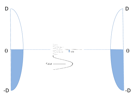
Figure 1: This figure depicts the density of states of the left and right contacts alongside with the density of states of the quantum dot in the final state schematically.

In this paper, we will investigate a scenario in which a molecular quantum dot is suddenly shifted from a position well below the Fermi level of the leads to a position where the Kondo effect is present by means of a gate voltage. Previous studies unambiguously demonstated that the strong electron-electron interactions give rise to a Kondo resonance pinned to the Fermi level of the contacts decorated with sidebands on each side due to the electron-phonon coupling. However, little is known about the real time electron dynamics of this system as a response to abrupt perturbations except a recent study using the mean field approximation for a spinless model RiwaretAl09PRB . The set-up of the system under consideration is shown schematically in Fig. 1. The goal of this paper is to fill this gap by reporting the instantaneous conductance after an interacting vibronic dot’s energy level has been moved to its final position.

II Theory

We model this device by a single spin degenerate level of energy $\epsilon_{dot}$ attached to leads through tunnel barriers and coupled to a single phonon mode. This model is referred as Holstein Hamiltonian. In this paper, we will be concerned with the strong electron-phonon coupling regime where the electron-phonon term can be discarded with a canonical transformation. We carry out the auxiliary boson transformation for the resulting Hamiltonian where the ordinary electron operator on the dot is rewritten in terms of a massless boson operator and a pseudofermion operator. $U$ $\rightarrow\infty$ limit is obtained by imposing the condition that the sum of the number of bosons and the pseudofermions is equal to unity.

The aforementioned Hamiltonian has three pieces describing the contacts, quantum dot and the tunneling process between them and it can be written as

$$H(t)=H_{C}+H_{D}(t)+H_{T}(t)$$ (1)

where

$$H_{C} = \sum_{k\alpha\sigma}(\epsilon_{k\alpha}-\mu_{\alpha})c^{\dagger}_{k\alpha\sigma}c_{k\alpha\sigma}$$

$$H_{D}(t) = \sum_{\sigma}[\epsilon_{dot}(t)+\lambda(a+a^{\dagger})]d^{\dagger}_{\sigma}d_{\sigma}+Ud^{\dagger}_{\uparrow}d_{\uparrow}d^{\dagger}_{\downarrow}d_{\downarrow}$$

$$+\omega_{0}a^{\dagger}a$$

$$H_{T}(t) = \sum_{k\alpha\sigma}(V_{k\alpha}(t)c^{\dagger}_{k\alpha\sigma}d_{\sigma}+h.c.).$$ (2)

In this Hamiltonian, $d_{\sigma}^{\dagger}(d_{\sigma})$ and $c_{k\alpha\sigma}^{\dagger}(c_{k\alpha\sigma})$ with $\alpha$=L,R create(annihilate) an electron of spin $\sigma$ in the quantum dot and in the left(L) and right(R) leads respectively. $V_{k\alpha}$ and $\mu_{\alpha}$ are the tunneling amplitudes and chemical potentials for the left and the right leads. $a^{{\dagger}}(a)$ creates(annihilates) a phonon within the quantum dot. $\lambda$ is the strength of the electron-phonon coupling and $\omega_{0}$ is the phonon frequency. In this paper, we will use atomic units with $\hbar=k_{B}=e=1$.

We will take the hopping matrix elements to be equal with no explicit time and energy dependence. Under this assumption, broadening of the dot level can be parameterized as $\Gamma(\epsilon)=\bar{\Gamma}\rho(\epsilon)$ where $\bar{\Gamma}$ is a constant given by $\bar{\Gamma}=2\pi|V(\epsilon_{f})|^{2}$ and $\rho(\epsilon)$ is the density of states function of the contacts. We will use parabolic density of states in both contacts with same bandwidth.

If the electron-phonon coupling is weak, electron-phonon coupling term can be treated perturbatively. In this paper, we will be concerned with the opposite case, where electron-phonon coupling is sufficiently strong compared to the tunnel couplings. In this regime, perturbative solution fails and a suitable canonical transformation must be applied to eliminate the electron-phonon coupling term. The most versatile choice is the unitary Lang-Firsov canonical transformation LangetAl63JETP given by

$$S=exp\left[\frac{\lambda}{\omega_{0}}\sum_{\alpha}d^{\dagger}_{\sigma}d_{\sigma}(a^{\dagger}-a)\right].$$ (3)

This transformation gives

$$SaS^{\dagger} = a-\frac{\lambda}{\omega_{0}}\sum_{\sigma}d^{\dagger}_{\sigma}d_{\sigma}$$

$$Sd_{\sigma}S^{\dagger} = d_{\sigma}X$$ (4)

where the operator $X$ is given by

$$X=exp\left[-\frac{\lambda}{\omega_{0}}(a^{\dagger}-a)\right].$$ (5)

The electron operators $d_{\sigma}(d^{\dagger}_{\sigma})$ in $H_{T}(t)$ are multiplied with $X(X^{\dagger})$ as a result of this transformation indicating that the tunneling electrons create and destroy a phonon cloud. This leads to polaron formation at the junction.

Under this canonical transformation, dot Hamiltonian turns into

$$\overline{H}_{D}(t) = SH_{D}(t)S^{\dagger}$$ (6)

$$= \sum_{\sigma}\left(\epsilon_{dot}(t)-\frac{\lambda^{2}}{\omega_{0}}\right)d^{\dagger}_{\sigma}d_{\sigma}$$

$$+\left(U-\frac{2\lambda^{2}}{\omega_{0}}\right)d^{\dagger}_{\uparrow}d_{\uparrow}d^{\dagger}_{\downarrow}d_{\downarrow}+\omega_{0}a^{\dagger}a.$$

It is clear from this result that the dot level and the Hubbard interaction strengths are renormalized as $\overline{\epsilon}_{dot}(t)=\epsilon_{dot}(t)-(\lambda^{2}/\omega_{0})$ and $\overline{U}=U-(2\lambda^{2}/\omega_{0})$ respectively as a result of this transformation.

In the strong electron-phonon coupling regime, i.e. when a polaron is formed at the junction, mean-field theory can be applied and the expectation value of operator X given by

$$<X>=exp\left[-\frac{\lambda^{2}}{\omega_{0}^{2}}\left(N_{ph.}+\frac{1}{2}\right)\right]$$ (7)

can serve as a substitute for the operator.

Even though $U$ has been renormalized to $\overline{U}=U-(2\lambda^{2}/\omega_{0})$, it is still positive and it overwhelms the line width $\Gamma$ for realistic systems. Hence, typically one takes $\overline{U}\rightarrow\infty$. This forbids double occupancy of the dot level. The downside of this advantage is that the standard diagrammatic techniques are not applicable anymore. This problem can be circumvented by introducing a massless boson operator and pseudofermion operator on the molecule. The original electron operators can be written in terms of these operators as

$$d_{\sigma}(t) = b^{\dagger}(t)f_{\sigma}(t)$$

$$d^{\dagger}_{\sigma}(t) = f^{\dagger}_{\sigma}(t)b(t)$$ (8)

subject to the requirement

$$Q=b^{\dagger}b+\sum_{\sigma}f^{\dagger}_{\sigma}f_{\sigma}=1,$$ (9)

which ensures the single occupancy of the dot level. The resulting slave boson Hamiltonian becomes

$$\overline{H}(t) = \sum_{k\alpha\sigma}(\epsilon_{k\alpha}-\mu_{\alpha})c^{\dagger}_{k\alpha\sigma}c_{k\alpha\sigma}+\sum_{\sigma}\overline{\epsilon}_{dot}f^{\dagger}_{\sigma}f_{\sigma}+\omega_{0}a^{\dagger}a$$ (10)

$$+\sum_{k\alpha\sigma}(\tilde{V}_{k\alpha}(t)c^{\dagger}_{k\alpha\sigma}f_{\sigma}b^{\dagger}+h.c.),$$

where the tunnel coupling and dot level are renormalized as $\tilde{V}_{k\alpha}(t)=V_{k\alpha}(t)<X>$ and $\overline{\epsilon}_{dot}(t)=\epsilon_{dot}(t)-(\lambda^{2}/\omega_{0})$ respectively.

We then invoke the well established non-crossing approximation(NCA) to determine the pseudofermion and slave boson self-energies. NCA has been shown to give accurate results for dynamical quantities save for temperatures below $T/T_{K}\approx$0.1 or finite magnetic fields. These two problematic cases will not be dwelled on in this paper.

The net current flowing through the device can be calculated from the resulting Green’s functions. We will write the net current as $I(t)=I_{L}(t)-I_{R}(t)$, where $I_{L}(t)(I_{R}(t))$ represents the net current from the left(right) contact through the left(right) barrier to the quantum dot. The most general expression for the net current JauhoetAl94PRB has previously been derived by using pseudofermion and slave boson Green’s functions GokeretAl07JPCM . Here, we will adapt it to the present situation. For symmetric coupling, the net current is reduced to

$$I(t)=-2\bar{\Gamma}Im(\int_{-\infty}^{t}dt_{1}G^{R}(t,t_{1})(f_{L}(t-t_{1})-f_{R}(t-t_{1})))$$ (11)

and the retarded Green function can be expressed as

$$G^{R}(t,t_{1}) = -i\theta(t-t_{1})[<d_{\sigma}(t)d^{\dagger}_{\sigma}(t_{1})><X(t)X^{\dagger}(t_{1})>$$ (12)

$$+<d^{\dagger}_{\sigma}(t_{1})d_{\sigma}(t)><X^{\dagger}(t_{1})X(t)>].$$

It turns out that the correlators of operators $X(t)$ and $X^{\dagger}(t_{1})$ can be evaluated precisely. They are given by $<X(t)X^{\dagger}(t_{1})>=e^{\phi(t_{1}-t)}$ and $<X^{\dagger}(t_{1})X(t)>=e^{\phi(t-t_{1})}$. In these expressions, the phase factor is given by

$$\phi(t_{1}-t) = -g[N_{ph.}(1-e^{-i\omega_{0}(t_{1}-t)})+$$ (13)

$$(N_{ph.}+1)(1-e^{i\omega_{0}(t_{1}-t)})],$$

where $g$ is defined as $g=\frac{\lambda^{2}}{\omega_{0}^{2}}$ and $N_{ph.}$, given by Bose-Einstein distribution $N_{ph.}=\frac{1}{e^{\frac{\hbar\omega_{0}}{k_{B}T}}-1}$ function, represents the average number of phonons for temperature $T$ and phonon frequency $\omega_{0}$. It has been pointed out before that the correlators are approximately equal only at sufficiently high temperatures such that $N_{ph.}$ is much larger than unity. At low temperatures, taking them equal may produce erroneous results such as producing phonon sidebands only on one side of the main Kondo peak. Therefore, in this paper we will not resort to such an approximation and keep the correlators in separate terms.

The retarded Green’s function can then be written as

$$G^{R}(t,t_{1}) = -i\theta(t-t_{1})[<d_{\sigma}(t)d^{\dagger}_{\sigma}(t_{1})>e^{\phi(t_{1}-t)}$$ (14)

$$+<d^{\dagger}_{\sigma}(t_{1})d_{\sigma}(t)>e^{\phi(t-t_{1})}]$$

$$= -i\theta(t-t_{1})[G^{>}_{real}(t,t_{1})e^{\phi(t_{1}-t)}$$

$$+G^{<}_{real}(t,t_{1})e^{\phi(t-t_{1})}].$$

Using the slave boson and pseudofermion decomposition of the original fermion operators on the molecule, the retarded Green’s function can be recasted as

$$G^{R}(t,t_{1}) = -i\theta(t-t_{1})[G^{R}_{pseudo}(t,t_{1})B^{<}(t_{1},t)e^{\phi(t_{1}-t)}$$ (15)

$$+G^{<}_{pseudo}(t,t_{1})B^{R}(t_{1},t)e^{\phi(t-t_{1})}]$$

The real-time coupled integro-differential Dyson equations for the retarded and less than Green’s functions are computed in a cartesian two-dimensional grid. The values are stored in a matrix and the matrix is propagated diagonally in time. The phase factors remain attached to the pseudofermion Green’s functions during this procedure in order to incorporate the phonon effects properly WerneretAl07PRL . The instantaneous conductance is obtained by performing an integration over the lowest row of the matrix using the expression

$$I(t) = 2\bar{\Gamma}Re(\int_{-\infty}^{t}dt_{1}(G_{pseudo}^{R}(t,t_{1})B^{<}(t_{1},t)e^{\phi(t_{1}-t)}$$ (16)

$$+G_{pseudo}^{<}(t,t_{1})B^{R}(t_{1},t)e^{\phi(t-t_{1})})\times$$

$$(f_{L}(t-t_{1})-f_{R}(t-t_{1}))),$$

where $f_{L}(t-t_{1})$ and $f_{R}(t-t_{1})$ are the convolution of the density of states function with the Fermi-Dirac distribution GokeretAl07JPCM . The conductance $G$ is equal to the current divided by the bias voltage. A comprehensive description of our numerical implementation has been published previously ShaoetAl194PRB ; IzmaylovetAl06JPCM .

An exquisite many-body state called the Kondo effect arises when the dot level is positioned below the Fermi energy at sufficiently low temperatures. The net spin localized within the dot and the Fermi sea of electrons in the contacts hybridize to form a spin singlet. This results in a sharp resonance fixed to the Fermi levels of the contacts in the dot density of states. The linewidth of the Kondo resonance can be approximated by an energy scale $T_{K}$ (Kondo temperature) given by

$$T_{K}\propto\left(\frac{D\Gamma}{4}\right)^{\frac{1}{2}}\exp\left(-\frac{\pi|\epsilon_{\rm dot}|}{\Gamma}\right),$$ (17)

where $D$ is a high energy cutoff equal to half bandwidth of the conduction electrons and $\Gamma$ corresponds to the value of coupling between the dot and the contacts $\Gamma(\epsilon)$ at $\epsilon=\epsilon_{F}$.

Our aim in this paper is to theoretically investigate a case in which the dot level is displaced from its equilibrium level abruptly by means of a gate voltage. We will be particularly interested in a system which has been studied before in the absence of any electron-phonon coupling. Its dot level is abruptly moved from $\epsilon_{dot}=-5\Gamma$ to $\epsilon_{dot}=-2\Gamma$ at $t=0$ where $\Gamma=\bar{\Gamma}\rho(\epsilon_{f})$. We will report the instantaneous conductance right after the dot is moved to its final position. In the following discussion, we will take the phonon frequency and the bandwidth as $\omega_{0}=0.06\Gamma$ and $D=9\Gamma$ respectively with $\Gamma$=0.4 eV.

III Results

We begin our analysis with the instantaneous conductance results immediately after the dot level has been switched to its final position. The results shown in Fig. 2 correspond to three different temperatures for a constant nonzero electron-phonon coupling $g$. Instantaneous conductance results in the absence of any electron-phonon coupling has been reported previously PlihaletAl05PRB . In Fig. 2, short timescale corresponds to $\Gamma$ t $<$ 10. The conductance oscillations related to the charge transfer in this timescale have already been analyzed in detail PlihaletAl05PRB ; MuhlbacheretAl08PRL , therefore we will not elaborate on them here. The Kondo timescale occurs between the end of the short timescale and attainment of a plateau by the instantaneous conductance. Kondo resonance starts developing in this timescale. It takes place roughly between 10 $<\Gamma$ t $<$ 60 in Fig. 2.

The first key feature that should be mentioned regarding Fig. 2 is that the steady state conductances (i.e. long time limit) are smaller than the case without any electron-phonon coupling for all temperatures as expected YangetAl10PLA . This anticipation stems from the fact that the electron-phonon coupling gradually quenches the Kondo effect GalperinetAl07PRB . This suppression has been explained with dephasing due to electron-phonon coupling and downward shift of the energy level as a result of phonon reorganization. The second effect is an obvious consequence of the renormalization of the dot level.

The second and more subtle effect is the sinusoidal oscillation of the current in the Kondo timescale. This effect is difficult to see in the main panel of Fig. 2, therefore in the inset, we show the magnification of the main panel with shifted conductance curves such that they overlap at the onset of oscillations. In the inset of Fig. 2, it is clear that the oscillation frequency is the same for all temperatures. Moreover, the amplitude of the oscillations decreases as the ambient temperature increases. It turns out that the oscillation frequency is equal to the phonon frequency $\omega_{0}$.

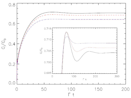
Figure 2: Black(solid), red(dashed) and blue(dash dotted) curves show instantaneous conductance results as a function of time for T=0.0009$\Gamma$, T=0.0010$\Gamma$ and $T$=0.0012$\Gamma$ respectively with $g$=2.25 after the dot level has been switched to its final position. The inset is the magnified version of the main panel. The curves for high temperatures in the inset have been shifted to enable camparison of the amplitudes.

In order to test the electron-phonon coupling strength dependency of the oscillation frequency, we increased $g$ and performed the previous calculation at the same temperatures. The result is shown in Fig. 3. First, the steady state conductance is lower for all temperatures for larger $g$. This is expected due to dephasing and downward level shift as pointed out above. On the other hand, conductance oscillations once more take place with a frequency equal to the phonon frequency $\omega_{0}$. We should mention that we increased $g$ in Fig. 3 by increasing $\lambda$ and keeping $\omega_{0}$ constant with respect to Fig. 2 to facilitate a direct comparison. It must be noted that changing the value of $\omega_{0}$ in our calculations again yields the oscillation frequency of the conductance as $\omega_{0}$. We checked that the oscillation frequency remains pinned to $\omega_{0}$ for all $g$ values.

We now want to study the amplitude of oscillations for various electron-phonon coupling strengths and temperatures in a systematic fashion. Fig. 4 shows the behaviour of amplitudes as a function of electron-phonon coupling strength at two different temperatures. The amplitude is zero at $g$=0 regardless of the temperature but it starts to increase gradually until it reaches a maximum before $g$=4. It then starts decreasing and it again approaches zero for large $g$ values. Meanwhile, the amplitude of oscillation is always larger at lower temperature for a given $g$. We verified that this conclusion holds for other temperatures as well.

It is of great interest to be able to provide a microscopic description for this peculiar behaviour of the transient current. One needs to resort to the spectral function of the dot to this end. This can be obtained by taking the Fourier transform of the retarded Green’s function. It has been shown before that the phonon sidebands are separated from the main Kondo peak by an integer multiple of phonon frequency $\omega_{0}$ ChenetAl05PRB ; GalperinetAl06PRB ; WangetAl07PRB ; PaaskeetAl05PRL . We propose that the sinusoidal oscillations seen in the transient current in the Kondo timescale are a result of an interference between the main Kondo peak and its phonon sidebands. For this reason, the frequency of oscillation was found to be equal to $\omega_{0}$. For a given $g$ parameter, the amplitude of oscillations increases as the temperature decreases because both the main Kondo peak and its phonon satellites are more developed at lower temperatures leading to stronger interference.

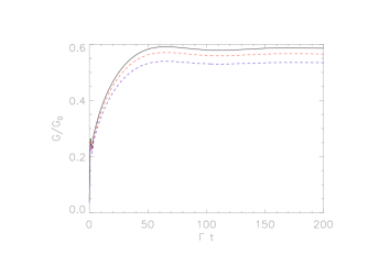
Figure 3: Black(solid), red(dashed) and blue(dash dotted) curves show instantaneous conductance results as a function of time for T=0.0009$\Gamma$, T=0.0010$\Gamma$ and $T$=0.0012$\Gamma$ respectively with $g$=3.75 after the dot level has been switched to its final position.

On the other hand, sweeping electron-phonon coupling strength at constant T gives rise to a more complicated situation as seen in Fig. 4. Even though the main Kondo peak is developed most fully for $g$=0 at a given temperature $T$ resulting in largest steady state conductance, no oscillation was detected in infinitesimal bias in Kondo timescale PlihaletAl05PRB because the phonon sidebands are completely absent in this case. Consequently, interference is nonexistent and oscillation amplitude is zero. For small $g$ values, amplitude of the oscillations gradually increases with $g$ because while the main Kondo peak pinned to the Fermi level gets inhibited a bit, its phonon sidebands become slightly more pronounced YangetAl10EPL . This naturally leads to stronger interference. Note that for $g<$0.5, the system is no longer in strong coupling regime. Still, our simulations show a consistent behaviour in this limit. The behaviour changes for moderate values of $g$. The amplitudes reach a maximum around $g$=4 and then start decreasing for larger $g$ values since destruction sets in for all peaks. Unsurprisingly, the amplitude goes to zero in large $g$ limit where the Kondo effect disappears completely and none of the peaks survives.

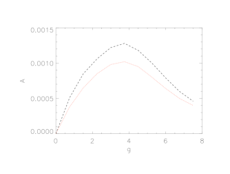
Figure 4: Black(dashed) and red(dotted) curves show amplitude of the second peak in conductance oscillation as a function of the electron-phonon coupling strength $g$ for $T$=0.0009$\Gamma$ and $T$=0.0010$\Gamma$ respectively. The amplitudes have been measured with respect to the steady state (i.e. $\Gamma$ t $\rightarrow\infty$) conductance values.

It is important to note that the oscillations take place exclusively with $\omega_{0}$ in infinitesimal bias and all the integer multiples of this frequency are completely absent as one can easily see from the Fourier transform of the instantaneous conductance in the long timescale shown in Fig. 5. This result is somewhat unexpected since the main Kondo peak should be interfering with other sidebands as well. This issue can be explained easily from an intuitive point of view. As one can see in Fig. 1 schematically and confirm by taking the Fourier transform of the retarded Green’s function, sidebands start getting drastically smaller away from the main Kondo peak resulting in less interference with it. Therefore, the oscillation amplitudes associated with these peaks is negligible compared to the one associated with the first sideband leading to the absence of other frequencies.

Before we conclude, we would like to address the effect of finite bias on the above reported time dependent conductance. First, it is well known that the bias would split the main elastic Kondo peak into two each of which are pinned to the Fermi level of the contacts. These split Kondo resonances would induce SKP oscillations in transient current with a frequency equal to the bias $V$ in the absence of any electron-phonon coupling PlihaletAl05PRB . Therefore, the effect of bias on the above system is two fold. First, steady state conductance would be lower than the infinitesimal bias case since the Kondo effect is gradually destroyed with bias. In fact, steady state investigation of a system with both strong electron-electron and electron-phonon interaction in finite bias showed that the differential conductance exhibits enhancements when the bias is an integer multiple of the phonon frequency $\omega_{0}$ PaaskeetAl05PRL . This is due to the fact that the inelastic phonon sidebands overlap with the split Kondo peaks. Indeed, this behaviour is reminiscent of the time averaged conductance of an ac driven quantum dot Goker08SSC .

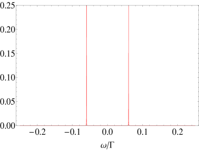
Figure 5: This figure shows the Fourier transform of the instantaneous conductance in the long timescale in infinitesimal bias.

In time dependent case, there are two interference effects taking place simultaneously, namely between the split main Kondo peaks and between each split main Kondo peak and its phonon sidebands. Obviously, this results in two distinct oscillation frequencies. This beating gives rise to more complicated oscillations in the transient current as seen in Fig. 6. When we take the Fourier transform of the transient current, we are able to identify these two distinct frequencies corresponding to the bias $V$ and the phonon frequency $\omega_{0}$. This result unambiguously confirms the validity of above interpretation. When the bias is an integer multiple of $\omega_{0}$, behaviour of the transient current is quite similar to zero bias case. In this case, only one frequency survives and it is equal to $\omega_{0}$.

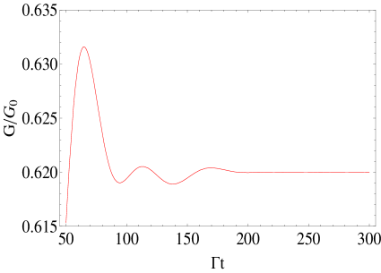
Figure 6: This figure shows the instantaneous conductance as a function of time for T=0.0009$\Gamma$ with $g$=2.25 and voltage bias of V=0.03$\Gamma$ after the dot level has been switched to its final position.

IV Conclusions

In conclusion, the non-crossing approximation was utilized in this paper to investigate the combined effect of strong electron-electron and electron-phonon interaction on instantaneous conductance in single molecule transistor when the dot level is suddenly shifted to a position where the Kondo resonance is present. Our results clearly showed that the instantaneous conductance displays decaying sinusoidal oscillations in the long timescale in infinitesimal bias. This fact set these novel oscillations apart from the previously predicted split Kondo peak oscillations PlihaletAl05PRB .

Investigation of the amplitude of these oscillations indicated that it sensitively depends on the ambient temperature and the electron-phonon coupling strength. Moreover, the frequency of these oscillations was found to be precisely equal to the phonon frequency upon taking the Fourier transform of the instantaneous conductance in the long timescale. Based on these observations and investigation of the density of states of the quantum dot, we proposed that the origin of this novel phenomenon can be attributed to the interference between the main elastic Kondo peak and its phonon sidebands. We also uncovered that finite source-drain bias results in more complicated fluctuation patterns in the instantaneous conductance. Two distinct frequencies corresponding to the phonon frequency $\omega_{0}$ and bias voltage $V$ play role in this case.

We believe the phenomenon discussed in this paper can be observed with present day ultrafast transient experimental techniques Teradaetal10JPCM since it takes place in the longest timescale which typically occurs on the order of tens of picoseconds. Besides, the theory presented here depicts a fairly realistic assessment of the single molecule junctions as it takes into account both Coulomb and vibrational interactions that are ubiquitous for real molecules, thus we hope to invigorate this field by motivating a new experiment with the predictions in this paper.

References

- (1) Aviram A and Ratner M A 1974 Chem. Phys. Lett. 29 277
- (2) Kroto H W, Heath J R, O’Brien S C, Curl S C and Smalley R E 1985 Nature 318 162
- (3) Ng T K and Lee P A 1988 Phys. Rev. Lett. 61 1768
- (4) Glazman L I and Raikh M E 1988 JETP Lett. 47 452
- (5) Goldhaber-Gordon D, Shtrikman H, Mahalu D, Abusch-Magder D, Meirav U and Kastner M A 1998 Nature 391 156–159
- (6) Goldhaber-Gordon D, Gores J, Kastner M A, Shtrikman H, Mahalu D and Meirav U 1998 Phys. Rev. Lett. 81 5225–5228
- (7) Cronenwett S M, Osterkamp T H and Kouwenhoven L P 1998 Science 281 540–544
- (8) Park J, Pasupathy A N, Goldsmith J I, Chang C, Yaish Y, Petta J R, Rinkoski M, Sethna J P, Abruna H D, McEuen P L and Ralph D C 2002 Nature 417 722
- (9) Liang W J, Shores M P, Bockrath M, Long J R and Park H 2002 Nature 417 725
- (10) Rocha A R, Garcia-Suarez V M, Bailey S W, Lambert C J, Ferrer J and Sanvito S 2005 Nature Materials 4 335
- (11) Seneor P, Bernand-Mantel A and Petroff F 2007 J. Phys.: Condens. Matter 19 165222
- (12) Kondo J 1964 Prog. Theor. Phys. 32 37
- (13) Hewson A C 1993 The Kondo Problem to Heavy Fermions (Cambridge: Cambridge University Press)
- (14) Ashoori R C 1996 Nature 379 413
- (15) Nordlander P, Pustilnik M, Meir Y, Wingreen N S and Langreth D C 1999 Phys. Rev. Lett. 83 808–811
- (16) Plihal M, Langreth D C and Nordlander P 2000 Phys. Rev. B 61 R13341–13344
- (17) Schiller A and Herschfield S 2000 Phys. Rev. B 62 R16271–R16274
- (18) Merino J and Marston J B 2004 Phys. Rev. B 69 115304
- (19) Plihal M, Langreth D C and Nordlander P 2005 Phys. Rev. B 71 165321
- (20) Anders F B and Schiller A 2005 Phys. Rev. Lett. 95 196801
- (21) Anders F B and Schiller A 2006 Phys. Rev. B 74 245113
- (22) Izmaylov A F, Goker A, Friedman B A and Nordlander P 2006 J. Phys.: Condens. Matter 18 8995–9006
- (23) Goker A, Friedman B A and Nordlander P 2007 J. Phys.: Condens. Matter 19 376206
- (24) Gull E, Werner P, Parcollet O and Troyer M 2008 Europhys. Lett. 82 57003
- (25) Werner P, Oka T and Millis A J 2009 Phys. Rev. B 79 035320
- (26) Schmidt T L, Werner P, Muhlbacher L and Komnik A 2008 Phys. Rev. B 78 235110
- (27) Galperin M, Ratner M A and Nitzan A 2007 J. Phys.: Condens. Matter 19 103201
- (28) Stipe B C, Rezaei M A and Ho W 1999 Phys. Rev. Lett. 82 1724
- (29) Hahn J R, Lee H J and Ho W 2000 Phys. Rev. Lett. 85 1914
- (30) Migdal A B 1958 Sov. Phys. JETP 7 996
- (31) Eliashberg G M 1960 Sov. Phys. JETP 11 696
- (32) Frederiksen T, Brandbyge M, Lorente N and Jauho A P 2004 Phys. Rev. Lett. 93 256601
- (33) Mii T, Tikhodeev S G and Ueba H 2003 Phys. Rev. B 68 205406
- (34) Galperin M, Ratner M A and Nitzan A 2004 Nano Lett. 4 1605
- (35) Galperin M, Ratner M A and Nitzan A 2004 J. Chem. Phys. 121 11965
- (36) Yu L H and Natelson D 2004 Nano Lett. 4 79
- (37) Zhu J X and Balatsky A V 2003 Phys. Rev. B 67 165326
- (38) Lundin U and McKenzie R H 2002 Phys. Rev. B 66 075303
- (39) Chen Z Z, Lu R and Zhu B F 2005 Phys. Rev. B 71 165324
- (40) Galperin M, Nitzan A and Ratner M A 2006 Phys. Rev. B 73 045314
- (41) Wang R Q, Zhou Y Q, Wang B and Xing D Y 2007 Phys. Rev. B 75 045318
- (42) Paaske J and Flensberg K 2005 Phys. Rev. Lett. 94 176801
- (43) Yong H C, Kai-Hua Y and Guang-Shan T 2007 Commun. Theor. Phys. 48 1107
- (44) Galperin M, Nitzan A and Ratner M A 2007 Phys. Rev. B 76 035301
- (45) Riwar R P and Schmidt T L 2009 Phys. Rev. B 80 125109
- (46) Lang I G and Firsov Y A 1963 Sov. Phys. JETP 16 1301
- (47) Jauho A P, Wingreen N S and Meir Y 1994 Phys. Rev. B 50 5528
- (48) Werner P and Millis A J 2007 Phys. Rev. Lett. 99 146404
- (49) Shao H X, Langreth D C and Nordlander P 1994 Phys. Rev. B 49 13929–13947
- (50) Muhlbacher L and Rabani E 2008 Phys. Rev. Lett. 100 176403
- (51) Yang K H, Zhao Y L, Wu Y J and Wu Y P 2010 Phys. Lett. A 374 2874
- (52) Yang K H, Wu Y P and Zhao Y L 2010 Europhys. Lett. 89 37008
- (53) Goker A 2008 Solid State Comm. 148 230
- (54) Terada Y, Yoshida S, Takeuchi O and Shigekawa H 2010 J. Phys.: Condens. Matter 22 264008