Abstract

We consider the classical superintegrable Hamiltonian system given by

$${\cal H}_{\lambda}={\cal T}+{\cal U}=\frac{\mathbf{p}^{2}}{2(1+{\lambda}\mathbf{q}^{2})}+\frac{\omega^{2}\mathbf{q}^{2}}{2(1+{\lambda}\mathbf{q}^{2})},$$

where $\cal U$ is known to be the “intrinsic” oscillator potential on the Darboux spaces of nonconstant curvature determined by the kinetic energy term $\cal T$ and parametrized by ${\lambda}$. We show that ${\cal H}_{\lambda}$ is Stäckel equivalent to the free Euclidean motion, a fact that directly provides a curved Fradkin tensor of constants of motion for ${\cal H}_{\lambda}$. Furthermore, we analyze in terms of ${\lambda}$ the three different underlying manifolds whose geodesic motion is provided by $\cal T$. As a consequence, we find that ${\cal H}_{\lambda}$ comprises three different nonlinear physical models that, by constructing their radial effective potentials, are shown to be two different nonlinear oscillators and an infinite barrier potential. The quantization of these two oscillators and its connection with spherical confinement models is briefly discussed.

PACS: 02.30.Ik 05.45.-a  45.20.Jj

KEYWORDS: superintegrability, deformation, hyperbolic, spherical, curvature, effective potential, Stäckel transform

1 Introduction

Let us consider the $N$-dimensional ($N$D) classical Hamiltonian defined by

$${\cal H}_{\lambda}={\cal T}(\mathbf{q},\mathbf{p})+{\cal U}(\mathbf{q})=\frac{\mathbf{p}^{2}}{2(1+{\lambda}\mathbf{q}^{2})}+\frac{\omega^{2}\mathbf{q}^{2}}{2(1+{\lambda}\mathbf{q}^{2})},$$ (1)

where ${\lambda}$ and $\omega$ are real parameters, and $\mathbf{q},\mathbf{p}\in\mathbb{R}^{N}$ are conjugate coordinates and momenta with canonical Poisson bracket $\{q_{i},p_{j}\}=\delta_{ij}$.

The mathematical and physical relevance of this system rely on two main properties [1]: (i) ${\cal H}_{\lambda}$ is a maximally superintegrable (MS) Hamiltonian, since it is endowed with the maximum possible number of $2N-1$ functionally independent integrals of motion; and (ii) the central potential ${\cal U}(\mathbf{q})$ can be interpreted as the “intrinsic” oscillator on the underlying curved manifold defined through the kinetic term $\cal T$. In particular, ${\cal T}$ determines the geodesic motion of a particle with unit mass on a conformally flat space which was constructed in [2, 3] and is the $N$D spherically symmetric generalization of the Darboux surface of type III [4, 5]. The corresponding metric and scalar curvature depend on ${\lambda}$ and are given by

$${\rm d}s^{2}=(1+{\lambda}\mathbf{q}^{2}){\rm d}\mathbf{q}^{2},\qquad R(\mathbf{q})=-{\lambda}\,\frac{(N-1)\bigl{(}2N+3(N-2){\lambda}\mathbf{q}^{2}\bigr{)}}{(1+{\lambda}\mathbf{q}^{2})^{3}}.$$ (2)

From this viewpoint, ${\cal H}_{\lambda}$ can be regarded as a MS “${\lambda}$-deformation” of the $N$D isotropic harmonic oscillator with frequency $\omega$ since $\lim_{{\lambda}\to 0}{\cal H}_{\lambda}=\frac{1}{2}\mathbf{p}^{2}+\frac{1}{2}\omega^{2}\mathbf{q}^{2}$.

We recall that ${\cal H}_{\lambda}$ can be identified as a particular case within other frameworks such as: (i) the “3D multifold Kepler” Hamiltonians [6, 7] (which generalize the MIC–Kepler and Taub-NUT systems); (ii) the “3D Bertrand systems” [8, 9, 10] (coming from a generalization of the classical Bertrand’s theorem [11] to curved spaces); and (iii) the “$N$D position-dependent mass systems” [12, 13, 14, 15, 16, 17, 18, 19, 20] (see also references therein) provided that the conformal factor of the metric (2) is identified with the variable mass function $m(\mathbf{q})=1+{\lambda}\mathbf{q}^{2}$.

The aim of this paper is twofold. On one hand, in the next section we provide a deeper insight in the set of integrals of motion of ${\cal H}_{\lambda}$ given in [1] by applying the so-called Stäckel transform or coupling constant metamorphosis [21, 22, 23, 24, 25]. In this way, we obtain the corresponding ${\lambda}$-deformation of the Fradkin tensor of integrals of motion [26] for the isotropic harmonic oscillator. On the other hand, we explicitly show that ${\cal H}_{\lambda}$ gives rise, in fact, to three different physical models. For this latter (and main) purpose, we present in section 3 which are the underlying manifolds that come out according to the values of ${\lambda}$. This analysis leads to three types of manifolds which, in turn, correspond to two nonlinear oscillator systems plus a barrier-like one, which are studied in section 4 by constructing their associated effective potential. The final result is that the Hamiltonian ${\cal H}_{\lambda}$ comprises the hyperbolic oscillator (${\lambda}>0$), the spherical one (the “interior” space with ${\lambda}<0$) and an infinite potential barrier (the “exterior” space with ${\lambda}<0$). Remarkably enough, the effective oscillator potentials are, in this order, hydrogen-like and oscillator-like, which means that the quantization of ${\cal H}_{\lambda}$ would provide different types of spherical confinement models like, for instance, [27, 28]. First results in this direction [29] are briefly sketched.

2 Superintegrability and the Stäckel transform

The MS property of ${\cal H}_{\lambda}$ is characterized by the following statement.

Theorem 1.

(i) The Hamiltonian ${\cal H}_{\lambda}$ (1), for any real value of ${\lambda}$, is endowed with the following constants of motion.

$\bullet$ $(2N-3)$ angular momentum integrals:

$$C^{(m)}=\!\!\sum_{1\leq i<j\leq m}\!\!\!\!(q_{i}p_{j}-q_{j}p_{i})^{2},\qquad C_{(m)}=\!\!\!\sum_{N-m<i<j\leq N}\!\!\!\!\!\!(q_{i}p_{j}-q_{j}p_{i})^{2},$$ (3)

where $m=2,\dots,N$ and $C^{(N)}=C_{(N)}$.

$\bullet$ $N^{2}$ integrals which form the ND curved Fradkin tensor:

$$I_{ij}=p_{i}p_{j}-\bigl{(}2{\lambda}{\cal H}_{\lambda}(\mathbf{q},\mathbf{p})-\omega^{2}\bigr{)}q_{i}q_{j},$$ (4)

where $i,j=1,\dots,N$ and such that ${\cal H}_{\lambda}=\frac{1}{2}\sum_{i=1}^{N}I_{ii}$.

(ii) Each of the three sets $\{{\cal H}_{\lambda},C^{(m)}\}$, $\{{\cal H}_{\lambda},C_{(m)}\}$ ($m=2,\dots,N$) and $\{I_{ii}\}$ ($i=1,\dots,N$) is formed by $N$ functionally independent functions in involution.

(iii) The set $\{{\cal H}_{\lambda},C^{(m)},C_{(m)},I_{ii}\}$ for $m=2,\dots,N$ with a fixed index $i$ is constituted by $2N-1$ functionally independent functions.

A restricted version of this result was proven in [1], where only the diagonal integrals $I_{ii}$ and the case ${\lambda}>0$ was considered. However, the same algebraic results do hold for ${\lambda}<0$, and this possibility enable us to get other physical systems different from the one with ${\lambda}>0$ that was solved in [1]. We also remark that the existence of a (curved) Fradkin tensor (4) is what makes ${\cal H}_{\lambda}$ (1) a distinguished Hamiltonian, that is, a MS one which can be regarded as the “closest neighbour of nonconstant curvature” to the harmonic oscillator system, which is obtained in the limit ${\lambda}\to 0$.

It is also worth stressing that theorem 1 can also be proven by relating ${\cal H}_{\lambda}$ with the free Euclidean motion through a Stäckel transform [21, 22, 23, 24, 25] as follows.

Let $H$ be an “initial” Hamiltonian, $H_{U}$ an “intermediate” one and ${\tilde{H}}$ the “final” system given by

$$H=\frac{\mathbf{p}^{2}}{\mu(\mathbf{q})}+V(\mathbf{q}),\qquad H_{U}=\frac{\mathbf{p}^{2}}{\mu(\mathbf{q})}+U(\mathbf{q}),\qquad\tilde{H}=\frac{H}{U}=\frac{\mathbf{p}^{2}}{\tilde{\mu}(\mathbf{q})}+\tilde{V}(\mathbf{q}),$$ (5)

such that

$$\tilde{\mu}=\mu U,\qquad\tilde{V}={V}/{U}.$$ (6)

Then, each second-order integral of motion (symmetry) $S$ of $H$ leads to a new one $\tilde{S}$ corresponding to $\tilde{H}$ through an “intermediate” symmetry $S_{U}$ of $H_{U}$. In particular, if $S$ and $S_{U}$ are given by

$$S=\sum_{i,j=1}^{N}a^{ij}(\mathbf{q})p_{i}p_{j}+W(\mathbf{q})=S_{0}+W(\mathbf{q}),\quad S_{U}=S_{0}+W_{U}(\mathbf{q}),$$ (7)

then we get a second-order symmetry of $\tilde{H}$ in the form

$$\tilde{S}=S_{0}-\frac{W_{U}}{U}\,H+\frac{1}{U}\,H.$$ (8)

In our case, we consider as the initial Hamiltonian $H$ (5) the free one on the $N$D Euclidean space minus a real constant $\alpha$ (related with ${\lambda}$ and $\omega$):

$$H=\frac{1}{2}\mathbf{p}^{2}-\alpha,\qquad 2{\lambda}\alpha=\omega^{2}.$$ (9)

And our aim is to perform a Stäckel transform to the Hamiltonian ${\cal H}_{\lambda}$ (1) but written in “final” form as

$${\tilde{H}}={\cal H}_{\lambda}-\alpha=\frac{1}{2}\left(\frac{\mathbf{p}^{2}-2\alpha}{1+{\lambda}\mathbf{q}^{2}}\right).$$ (10)

Thus it can be checked that the transformation works provided that

$$\mu=2,\quad V=-\alpha,\quad\tilde{\mu}=2(1+{\lambda}\mathbf{q}^{2}),\quad\tilde{V}=\frac{-\alpha}{1+{\lambda}\mathbf{q}^{2}},\quad U=(1+{\lambda}\mathbf{q}^{2}),$$ (11)

and the intermediate Hamiltonian is the $N$D istropic harmonic oscillator

$$H_{U}=\frac{1}{2}\mathbf{p}^{2}+{\lambda}\mathbf{q}^{2}+1.$$ (12)

Next we consider the symmetries $S$ of $H$ (9) which is clearly MS and endowed with $2N-1$ functionally independent functions. Some of them are exactly (3):

$$S^{(m)}=\!\!\sum_{1\leq i<j\leq m}\!\!\!\!(q_{i}p_{j}-q_{j}p_{i})^{2},\qquad S_{0}^{(m)}=C^{(m)},\qquad W^{(m)}=0,$$

$$S_{(m)}=\!\!\sum_{N-m<i<j\leq N}\!\!\!\!\!\!(q_{i}p_{j}-q_{j}p_{i})^{2},\qquad S_{0,{(m)}}=C_{(m)},\qquad W_{(m)}=0,$$

$$S_{ij}=p_{i}p_{j},\qquad S_{0,ij}=p_{i}p_{j},\qquad W_{ij}=0,$$ (13)

where $m=2,\dots,N$ and $i,j=1,\dots N$. The symmetries $S_{U}$ of $H_{U}$ (12) read

$$S_{U}^{(m)}\equiv S^{(m)},\qquad S_{0}^{(m)}=C^{(m)},\qquad W_{U}^{(m)}=0,$$

$$S_{U,(m)}\equiv S_{(m)},\qquad S_{0,{(m)}}=C_{(m)},\qquad W_{U,(m)}=0,$$

$$S_{U,ij}=p_{i}p_{j}+2{\lambda}q_{i}q_{j},\qquad S_{0,ij}=p_{i}p_{j},\qquad W_{U,ij}=2{\lambda}q_{i}q_{j}.$$ (14)

Consequently the Hamiltonian ${\tilde{H}}$ (10) is also MS and its integrals of motion $\tilde{S}$ (8) turn out to be

$$\tilde{S}^{(m)}=\!\!\sum_{1\leq i<j\leq m}\!\!\!\!(q_{i}p_{j}-q_{j}p_{i})^{2}+\tilde{H}=C^{(m)}+\tilde{H},$$

$$\tilde{S}_{(m)}=\!\!\sum_{N-m<i<j\leq N}\!\!\!\!\!\!(q_{i}p_{j}-q_{j}p_{i})^{2}+\tilde{H}=C_{(m)}+\tilde{H},$$

$$\tilde{S}_{ij}=p_{i}p_{j}-2{\lambda}q_{i}q_{j}\tilde{H}+\tilde{H}.$$ (15)

Finally by introducing $\tilde{H}={\cal H}_{\lambda}-\alpha$ we recover all the results given in theorem 1 proving that, in fact, the Hamiltonian ${\cal H}_{\lambda}$ is Stäckel equivalent to the free Euclidean motion.

3 The underlying Darboux manifolds

We recall that the real parameter ${\lambda}=1/\kappa$ was restricted in [1] to take a positive value. Clearly, the superintegrability properties of the Hamiltonian stated in theorem 1 do hold for a negative ${\lambda}$ as well. Nevertheless the underlying space and the oscillator potential change dramatically with the sign of ${\lambda}$ in such a manner that the domain of the Hamiltonian must be restricted when ${\lambda}<0$. Hence, the “generic” Darboux space (that is, the Riemannian manifold with metric (2) determined by the kinetic part of (1)) leads to three different manifolds ${\mathcal{M}}^{N}$ which have the following geometric and topological properties.

3.1 Type ${\rm I}$: ${\lambda}>0$

The Darboux space is the complete Riemannian manifold ${\mathcal{M}}^{N}=(\mathbb{R}^{N},g)$, with metric $g_{ij}:=(1+{\lambda}\mathbf{q}^{2})\,\delta_{ij}$. The scalar curvature $R(r)\equiv R(|\mathbf{q}|)$ (2) is always a negative increasing function such that $\lim_{r\to\infty}R=0$ and it has a minimum at the origin

$$R(0)=-2{\lambda}N(N-1),$$

which is exactly the scalar curvature of the $N$D hyperbolic space with negative constant sectional curvature equal to $-2{\lambda}$.

3.2 Type ${\rm II}$: ${\lambda}<0$ restricted to the interior space

In this case we consider the interior Darboux space defined by ${\mathcal{M}}^{N}=(B_{{r_{\rm c}}},g)$ such that

$$g_{ij}:=(1-|{\lambda}|\mathbf{q}^{2})\,\delta_{ij},\qquad B_{r_{\rm c}}=[0,{r_{\rm c}}),\qquad{r_{\rm c}}=|\mathbf{q}|_{\rm c}=1/\sqrt{|{\lambda}|},$$

that is, $B_{r_{\rm c}}$ denotes the ball centered at $0$ of radius ${r_{\rm c}}$ which is the critical or singular value for which $R(r)$ diverges and $\lim g_{r\to{r_{\rm c}}^{-}}=0$. It is clear that ${\mathcal{M}}^{N}$ is incomplete as a Riemannian manifold. Notice also that

$$R(0)=2|{\lambda}|N(N-1),$$

which coincides with the the scalar curvature of the $N$D spherical space with positive constant sectional curvature equal to $2|{\lambda}|$. The behavior of $R(r)$ depends on the dimension $N$ as follows.

• When $2\leq N\leq 6$, the scalar curvature is a positive increasing function such that ${\lim_{r\to r^{-}_{\rm c}}R(r)=+\infty}$.

• If $7\leq N$, there is a positive maximum for $R(r)$ corresponding to

  $$r_{\rm max}=\sqrt{\frac{N+2}{2(N-2)|{\lambda}|}},\qquad R(r_{\rm max})=\frac{4|{\lambda}|(N-1)(N-2)^{3}}{(N-6)^{2}},$$

  and ${\lim_{r\to r^{-}_{\rm c}}R(r)=-\infty}$.

3.3 Type ${\rm III}$: ${\lambda}<0$ restricted to the exterior space

To consider the exterior Darboux space, ${\mathcal{M}}^{N}=(\mathbb{R}^{N}\backslash\overline{B_{{r_{\rm c}}}},g)$, requires to change the sign of both the metric and scalar curvature (2):

$$g_{ij}:=(|{\lambda}|\mathbf{q}^{2}-1)\,\delta_{ij},\quad\mathbb{R}^{N}\backslash\overline{B_{{r_{\rm c}}}}=({r_{\rm c}},\infty),$$

$$R(\mathbf{q})=|{\lambda}|\,\frac{(N-1)\bigl{(}2N-3(N-2)|{\lambda}|\mathbf{q}^{2}\bigr{)}}{(|{\lambda}|\mathbf{q}^{2}-1)^{3}}.$$

Note that ${\mathcal{M}}^{N}$ is again incomplete. According to the dimension $N$, the function $R(r)$ behaves as follows:

• For $N=2$, this is a positive decreasing function such that ${\lim_{r\to r^{+}_{\rm c}}R(r)=+\infty}$ and ${\lim_{r\to\infty}R(r)=0}$.

• If $3\leq N\leq 5$, the scalar curvature has a negative minimum

  $$r_{\rm min}=\sqrt{\frac{N+2}{2(N-2)|{\lambda}|}},\qquad R(r_{\rm min})=-\frac{4|{\lambda}|(N-1)(N-2)^{3}}{(N-6)^{2}},$$

  with ${\lim_{r\to r^{+}_{\rm c}}R(r)=+\infty}$ and ${\lim_{r\to\infty}R(r)=0}$.

• When $6\leq N$, $R(r)$ is a negative increasing function with ${\lim_{r\to r^{+}_{\rm c}}R(r)=-\infty}$ and ${\lim_{r\to\infty}R(r)=0}$.

4 Three radial systems and their effective potentials

Firstly, we remark that ${\cal H}_{\lambda}$ can also be expressed in terms of hyperspherical coordinates $r,\theta_{j}$, and canonical momenta $p_{r},p_{\theta_{j}}$, $(j=1,\dots,N-1)$ defined by

$$q_{j}=r\cos\theta_{j}\prod_{k=1}^{j-1}\sin\theta_{k},\quad 1\leq j<N,\qquad q_{N}=r\prod_{k=1}^{N-1}\sin\theta_{k},$$ (16)

so, $r=|\mathbf{q}|$. Thus the Hamiltonian (1) reduces to a 1D radial system:

$${\cal H}_{\lambda}(r,p_{r})=\frac{p_{r}^{2}+r^{-2}\mathbf{L}^{2}}{2(1+{\lambda}r^{2})}+\frac{\omega^{2}r^{2}}{2(1+{\lambda}r^{2})}={\cal T}(r,p_{r})+{\cal U}(r),$$ (17)

where $\mathbf{L}^{2}\equiv C^{(N)}\equiv C_{(N)}$ is the total angular momentum given by

$$\mathbf{L}^{2}=\sum_{j=1}^{N-1}p_{\theta_{j}}^{2}\prod_{k=1}^{j-1}\frac{1}{\sin^{2}\theta_{k}}.$$ (18)

Now, the geometric analysis performed in the previous section indicates that we must deal with three different physical systems that, for the types I and II we name nonlinear hyperbolic oscillator and nonlinear spherical oscillator, respectively. In these two cases the generic expression for the Hamiltonian (1) is kept (with the boundary ${r_{\rm c}}$ for type II), while for type III the sign of the Hamiltonian has to be reversed, thus ensuring a positive kinetic term (and provided that the corresponding restriction on the domain is considered). In particular, as far as the nonlinear radial potential ${\cal U}(r)$ (17) is concerned we point out the following facts:

$\bullet$ Nonlinear hyperbolic oscillator. When ${\lambda}>0$, the potential is a positive increasing function, such that

$${\cal U}(r)=\frac{\omega^{2}r^{2}}{2(1+{\lambda}r^{2})},\qquad{\cal U}(0)=0,\qquad\mbox{and}\qquad\lim_{r\to\infty}{\cal U}(r)=\frac{\omega^{2}}{2{\lambda}}.$$ (19)

$\bullet$ Nonlinear spherical oscillator. If ${\lambda}<0$ and $r<{r_{\rm c}}$, the potential is also a positive increasing function verifying

$${\cal U}(r)=\frac{\omega^{2}r^{2}}{2(1-|{\lambda}|r^{2})},\qquad{\cal U}(0)=0,\qquad\mbox{and}\qquad\lim_{r\to{r_{\rm c}}^{-}}{\cal U}(r)=+\infty.$$ (20)

$\bullet$ Exterior potential. When ${\lambda}<0$ and ${r_{\rm c}}<r$ we impose the change of the sign of the Hamiltonian. In this way the potential becomes a positive decreasing function:

$${\cal U}(r)=\frac{\omega^{2}r^{2}}{2(|{\lambda}|r^{2}-1)},\qquad\lim_{r\to{r_{\rm c}}^{+}}{\cal U}(r)=+\infty,\qquad\lim_{r\to\infty}{\cal U}(r)=\frac{\omega^{2}}{2|{\lambda}|}.$$ (21)

But it is essential to stress that each of the above potentials has to be considered on the corresponding curved space described in section 3. In this respect, the complete classical system can be better understood by introducing an effective potential (EP) that takes into account each curved background. This can be achieved by applying a 1D canonical transformation [29]

$$P=P(r,p_{r}),\qquad Q=Q(r),\qquad\{Q,P\}=1,$$

on the 1D radial Hamiltonian (17) yielding

$${\cal H}_{\lambda}(Q,P)=\frac{1}{2}P^{2}+{\cal U}_{\rm eff}(Q).$$

Next we present such an effective potential for the three abovementioned systems.

4.1 The nonlinear hyperbolic oscillator

The 1D canonical transformation is defined by

$$P(r,p_{r})=\frac{p_{r}}{\sqrt{1+{\lambda}r^{2}}},\qquad Q(r)=\frac{1}{2}r\sqrt{1+{\lambda}r^{2}}+\frac{{\rm arc}\!\sinh(\sqrt{{\lambda}}r)}{2\sqrt{{\lambda}}},$$ (22)

which implies that $Q(r)$ has a unique (continuously differentiable) inverse $r(Q)$, on the whole positive semiline, that is, both $r,Q\in[0,\infty)$; note that ${\rm d}Q(r)=\sqrt{1+{\lambda}r^{2}}{\rm d}r$. This transformation yields the EP

$${\cal U}_{\rm eff}(Q(r))=\frac{c_{N}}{2(1+{\lambda}r^{2})r^{2}}+\ \frac{\omega^{2}r^{2}}{2(1+{\lambda}r^{2})},$$ (23)

where $c_{N}\geq 0$ is the value of the integral of motion corresponding to the square of the total angular momentum $C_{(N)}\equiv\mathbf{L}^{2}$ (18). Hence the radial motion of the system can be described as the 1D problem given by the potential ${\cal U}_{\rm eff}(Q(r))$.

In fact, ${\cal U}_{\rm eff}$ is always positive and it has a minimum located at $r_{\rm min}$ such that

$$r^{2}_{\rm min}=\frac{{\lambda}c_{N}+\sqrt{{\lambda}^{2}c_{N}^{2}+\omega^{2}c_{N}}}{\omega^{2}},\quad{\cal U}_{\rm eff}(Q(r_{\min}))=-{\lambda}c_{N}+\sqrt{{\lambda}^{2}c_{N}^{2}+\omega^{2}c_{N}}.$$ (24)

Therefore, $r_{\rm min}$ and ${\cal U}_{\rm eff}(Q(r_{\min}))$ are, respectively, greater and smaller than those corresponding to the isotropic harmonic oscillator, which are

$${\lambda}=0\rightarrow\quad r^{2}_{\rm min}={\sqrt{c_{N}}}/{\omega},\qquad{\cal U}_{\rm eff}(Q(r_{\min}))=\omega\sqrt{c_{N}}.$$ (25)

This EP has two representative limits:

$$\lim_{r\to 0}{\cal U}_{\rm eff}(Q(r))=+\infty,\qquad\lim_{r\to\infty}{\cal U}_{\rm eff}(Q(r))={\omega^{2}}/({2{\lambda}}),$$ (26)

the latter being coincident with (19). Thus, this EP is hydrogen-like (see fig. 1).

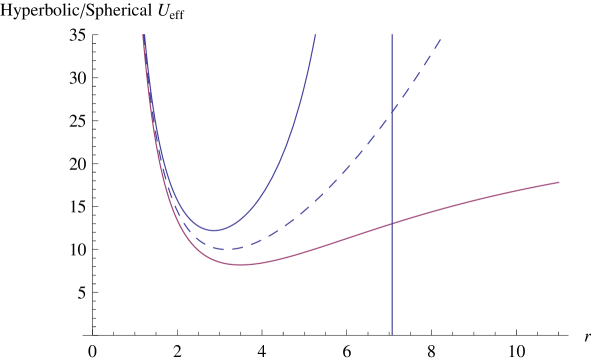
Figure 1: The effective nonlinear hyperbolic and spherical oscillator potentials (23) and (29) for ${\lambda}=\pm 0.02$, $c_{N}=100$ and $\omega=1$. The minimum of the hyperbolic potential (red curve) is located at $r_{\rm min}=3.49$ with ${\cal U}_{\rm eff}(r_{\rm min})=8.2$ and ${\cal U}_{\rm eff}(\infty)=25$, while the minimum of the spherical one (blue curve) is located at $r_{\rm min}=2.86$ with ${\cal U}_{\rm eff}(r_{\rm min})=12.2$ and ${r_{\rm c}}=7.07$. The dashed line corresponds to the effective potential of the harmonic oscillator with ${\lambda}=0$ with minimum ${\cal U}_{\rm eff}(r_{\rm min})=10$ at $r_{\rm min}=3.16$.

4.2 The nonlinear spherical oscillator

In this case, the canonical transformation is given by

$$P(r,p_{r})=\frac{p_{r}}{\sqrt{1-|{\lambda}|r^{2}}},\qquad Q(r)=\frac{1}{2}r\sqrt{1-|{\lambda}|r^{2}}+\frac{{\rm arc}\!\sin(\sqrt{|{\lambda}|}r)}{2\sqrt{|{\lambda}|}},$$ (27)

so that $Q(r)$ has a unique inverse $r(Q)$ on the intervals

$$r\in\left[0,{r_{\rm c}}\right),\quad{r_{\rm c}}=\frac{1}{\sqrt{|{\lambda}|}};\qquad Q\in\left[0,Q_{\rm c}\right),\quad Q_{\rm c}=\frac{\pi}{4\sqrt{|{\lambda}|}}.$$ (28)

The EP reads

$${\cal U}_{\rm eff}(Q(r))=\frac{c_{N}}{2(1-|{\lambda}|r^{2})r^{2}}+\frac{\omega^{2}r^{2}}{2(1-|{\lambda}|r^{2})},$$ (29)

which is always positive and it has a minimum located at $r_{\rm min}$ such that

$$r^{2}_{\rm min}=\frac{-|{\lambda}|c_{N}+\sqrt{{\lambda}^{2}c_{N}^{2}+\omega^{2}c_{N}}}{\omega^{2}},\quad{\cal U}_{\rm eff}(Q(r_{\min}))=|{\lambda}|c_{N}+\sqrt{{\lambda}^{2}c_{N}^{2}+\omega^{2}c_{N}}.$$ (30)

But now $r_{\rm min}$ and ${\cal U}_{\rm eff}(Q(r_{\min}))$ are, respectively, smaller and greater than those corresponding to the isotropic harmonic oscillator (25). This EP has again two characteristic limits:

$$\lim_{r\to 0}{\cal U}_{\rm eff}(Q(r))=+\infty,\qquad\lim_{r\to{r_{\rm c}}^{-}}{\cal U}_{\rm eff}(Q(r))=+\infty,$$ (31)

which means that we have a deformed oscilator potential that goes smoothly to an infinite barrier as $r$ approaches ${r_{\rm c}}^{-}$ (see fig. 1).

4.3 The exterior potential

The canonical transformation for the third system turns out to be

$$P(r,p_{r})=\frac{p_{r}}{\sqrt{|{\lambda}|r^{2}-1}},\quad Q(r)=\frac{1}{2}r\sqrt{|{\lambda}|r^{2}-1}-\frac{\ln\left(2\left({|{\lambda}|}r+\sqrt{|{\lambda}|}\sqrt{|{\lambda}|r^{2}-1}\right)\right)}{2\sqrt{|{\lambda}|}}$$ (32)

and $Q(r)$ has a unique inverse $r(Q)$ on the intervals

$$r\in\left[{r_{\rm c}},\infty\right),\quad{r_{\rm c}}=\frac{1}{\sqrt{|{\lambda}|}};\qquad Q\in\left[Q_{\rm c},\infty\right),\quad Q_{\rm c}=-\frac{\ln\left(2(\sqrt{|{\lambda}|}r\right)}{2\sqrt{|{\lambda}|}}.$$ (33)

The EP is

$${\cal U}_{\rm eff}(Q(r))=\frac{c_{N}}{2(|{\lambda}|r^{2}-1)r^{2}}+\frac{\omega^{2}r^{2}}{2(|{\lambda}|r^{2}-1)}.$$ (34)

The function ${\cal U}_{\rm eff}$ is again positive but, unlike the two previous systems, it has no minimum; this fulfils the same limits (21) so EP is an infinite (left) potential barrier which is represented in fig. 2.

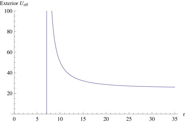
Figure 2: The effective nonlinear exterior oscillator potential (34) for ${\lambda}=-0.02$, $c_{N}=100$ and $\omega=1$. The critical point is ${r_{\rm c}}=7.07$ and ${\cal U}_{\rm eff}(\infty)=25$

Finally, some remarks concerning the quantization of these systems are in order. The nonlinear hyperbolic oscillator $({\lambda}>0)$ has been fully quantized in [29] and its discrete spectrum is given by

$$E_{n}=-\hbar^{2}\lambda\left(n+\frac{N}{2}\right)^{2}+\hbar\left(n+\frac{N}{2}\right)\sqrt{\hbar^{2}\lambda^{2}\left(n+\frac{N}{2}\right)^{2}+\omega^{2}}.$$ (35)

The corresponding stationary states have been obtained in analytic form. Note that the limit $n\to\infty$ of $E_{n}$ is just the asymptotic value ${\omega^{2}}/{2{\lambda}}$, as expected.

In view of the shape of the effective potential (see fig. 1), the quantum spherical oscillator $({\lambda}<0)$ should provide a new radial confinement model that could be useful as a position-dependent-mass model for spherical quantum dots [30]. The exact solution of the corresponding Schrödinger problem is still in progress.

References

- [1] Ballesteros A., Enciso A., Herranz F.J., Ragnisco O.: Physica D 237, (2008) 505
- [2] Ballesteros A., Enciso A., Herranz F.J., Ragnisco O.: Phys. Lett. B 652, (2007) 376
- [3] Ballesteros A., Enciso A., Herranz F.J., Ragnisco O.: Ann. Phys. 324, (2009) 1219
- [4] Koenigs G.: in Leçons sur la théorie générale des surfaces, vol. 4, ed. Darboux G., Chelsea, New York (1972) 368
- [5] Kalnins E.G., Kress J.M., Miller W. Jr., Winternitz P.: J. Math. Phys. 44, (2003) 5811
- [6] Iwai T., Katayama N.: J. Math. Phys. 36, (1995) 1790
- [7] Iwai T., Uwano Y., Katayama N.: J. Math. Phys. 37, (1996) 608
- [8] Perlick V.: Class. Quantum Grav. 9, (1992) 1009
- [9] Ballesteros A., Enciso A., Herranz F.J., Ragnisco O.: Class. Quantum Grav. 25, (2008) 165005
- [10] Ballesteros A., Enciso A., Herranz F.J., Ragnisco O.: Commun. Math. Phys. 290, (2009) 1033
- [11] Bertrand J.: C. R. Acad. Sci. Paris 77, (1873) 849
- [12] von Roos O.: Phys. Rev. B 27, (1983) 7547
- [13] Lévy-Leblond J.M.: Phys. Rev. A 52, (1995) 1845
- [14] Chetouani L., Dekar L., Hammann T.F.: Phys. Rev. A 52, (1995) 82
- [15] Plastino A.R., Rigo A., Casas M., Gracias F., Plastino A.: Phys. Rev. A 60, (1999) 4318
- [16] Quesne C., Tkachuk V.M.: J. Phys. A: Math. Gen. 37, (2004) 4267
- [17] Bagchi B., Banerjee A., Quesne C., Tkachuk V.M.: J. Phys. A: Math. Gen. 38, (2005) 2929
- [18] Quesne C.: Ann. Phys. 321, (2006) 1221
- [19] Gadella M., Kuru S., Negro J.: Phys. Lett. A. 362, (2007) 265
- [20] S. Cruz y Cruz, J. Negro, L.M. Nieto: Phys. Lett. A 369, (2007) 400
- [21] Hietarinta J., Grammaticos B., Dorizzi B., Ramani A.: Phys. Rev. Lett. 53, (1984) 1707
- [22] Kalnins E.G., Kress J.M,, Miller W. Jr.: J. Math. Phys. 46, (2005) 053510
- [23] Kalnins E.G., Kress J.M,, Miller W. Jr.: J. Math. Phys. 47, (2006) 043514
- [24] Sergyeyev A., Blaszak M.: J. Phys. A: Math. Theor. 41, (2008) 105205
- [25] Kalnins E.G., Miller W. Jr., Post S.: J. Phys. A: Math. Theor. 43, (2010) 035202
- [26] Fradkin D.M.: Amer. J. Phys. 33, (1965) 207
- [27] Al-Jaber S.M.: Int. J. Theor. Phys. 47, (2008) 1853
- [28] Montgomery Jr. H.E., Campoy G., Aquino N.: Phys. Scr. 81, (2010) 045010
- [29] Ballesteros A., Enciso A., Herranz F.J., Ragnisco O., Riglioni D.: (2010) arXiv:1007.1335
- [30] Gritsev V.V., Kurochkin Y.A.: Phys. Rev. B 64, (2001) 035308