The Bäcklund Transform of
Principal Contact Element Nets

Abstract.

We investigate geometric aspects of the the Bäcklund transform of principal contact element nets. A Bäcklund transform exists if and only if it the principal contact element net is of constant negative Gaussian curvature (a pseudosphere). We describe an elementary construction of the Bäcklund transform and prove its correctness. Finally, we show that Bianchi’s Permutation Theorem remains valid in our discrete setting.

1. Introduction

In the 1880s A. V. Bäcklund and L. Bianchi explored the transformation of one surface of constant negative Gaussian curvature (a pseudosphere) into a surface of the same constant Gaussian curvature. These surface transformations were named after Bäcklund and, in their formulation in the language of partial differential equations, play an important role in soliton theory and in integrable systems. We refer the reader to the monograph [10] for a comprehensive modern treatment with many applications.

In 1952, W. Wunderlich gave a geometric description of the Bäcklund transform of a discrete structure that is nowadays called a K-net — a discrete asymptotic net of constant negative Gaussian curvature [14]. Later, analytic formulations were added and the discrete transformations were embedded into the theory of Discrete Differential Geometry, see the monograph [4].

In this article we perform a comprehensive geometric study of the Bäcklund transform of principal contact element nets — nets of contact elements such that any two neighbouring contact elements have a common tangent sphere. Our main results are original but there exist related contributions in the above mentioned publications. We also have to mention the article [11] by W. Schief. It contains a description of the Bäcklund transform of discrete O-surfaces. While the vertex sets of discrete O-surfaces and principal contact element nets are identical (both are circular nets), the normals differ. For O-surfaces, they are defined by a simple algebraic condition, for principal contact element nets they satisfy a geometric criterion. Accordingly, our approach is of geometric nature as opposed to Schief’s analytic treatment.

Our results are natural extensions of recent works in discrete kinematics [13, 12]. While their formulation is rather natural at this point, some of our proofs tend to be rather involved and require extensive calculations. We partly attribute this to the observation that a (smooth or discrete) asymptotic parametrization is more appropriate for the description of Bäcklund transforms. Principal contact element nets discretize principal parametrizations and lead to spatial structures of complicated nature.

The occasional use of a computer algebra system (CAS) is indispensable in this work. We use Maple 13 for this purpose. In order to make the computer calculations understandable, we try to give rather explicit descriptions.

2. Preliminaries and statement of main results

We proceed by giving definitions for the main concepts, by stating our central results and by clarifying their relations. Proofs are deferred to later sections.

Principal contact element nets provide a rich discrete surface representation, consisting of points and normal vectors. They have been introduced in [3] in an attempt to develop a common master theory for circular nets (see [4, Section 3.5]) and conical nets (see [4, Section 3.4] and [9]).

Definition 1.

A contact element is a pair $(p,\mathbf{n})$ consisting of a point $a\in E^{3}$ (Euclidean three-space) and a unit vector $\mathbf{n}\in\mathbb{R}^{3}$. Its normal line $N$ is the oriented straight line through $a$ and in direction of $\mathbf{n}$, its oriented tangent plane $\pi$ is the plane through $p$ with oriented normal vector $\mathbf{n}$.

In this text we will always denote normal vector and normal line by the same letter but in different fonts: Lowercase, boldface for vectors, uppercase, italic for lines — just as in Definition 1.

Definition 2.

A contact element net is a map $(p,\mathbf{n})$ from $\mathbb{Z}^{d}$, $d\geq 2$, to the space of contact elements. A principal contact element net is a contact element net such that any two neighbouring contact elements $(p_{i},\mathbf{n}_{i})$ and $(p_{j},\mathbf{n}_{j})$ have a common oriented tangent sphere.

The defining condition of principal contact element nets is rather restrictive. It implies that neighbouring normal lines $N_{i}$ and $N_{j}$ intersect in a common point $h_{ij}$ which is at the same oriented distance from both vertices $p_{i}$ and $p_{j}$. This shows that neighbouring contact elements have a bisector plane $\beta_{ij}$. Moreover, the vertices of an elementary quadrilateral lie on a circle, the tangent planes are tangent to a cone of revolution and the normal lines form a skew quadrilateral on a hyperboloid of revolution.

An elementary quadrilateral $(p_{0},\mathbf{n}_{0})$, $(p_{1},\mathbf{n}_{1})$, $(p_{2},\mathbf{n}_{2})$, $(p_{3},\mathbf{n}_{3})$ of a principal contact element net can be constructed by choosing the vertices $p_{0}$, $p_{1}$, $p_{2}$, and $p_{3}$ on a circle, prescribin $\mathbf{n}_{0}$ and then finding the other normal vectors by reflection in the bisector planes $\beta_{i,i+1}$ of $p_{i}$ and $p_{i+1}$.

In this article we investigate principal contact element nets that admit a Bäcklund transform:

Definition 3.

Two principal contact element nets $(p,\mathbf{n})$ and $(q,\mathbf{m})$ are called Bäcklund mates if

1. The distance of corresponding points $p_{i}$ and $q_{i}$ is constant.

2. The angle of corresponding normals $\mathbf{n}_{i}$ and $\mathbf{m}_{i}$ is constant. (It is necessary to measure this angle consistently in counter-clockwise direction when viewed along the ray from $p_{i}$ to $q_{i}$.)

3. Two corresponding tangent planes $\pi_{i}$ and $\chi_{i}$ intersect in the connecting line $p_{i}\vee q_{i}$ of their vertices.

In this case, $(q,\mathbf{m})$ is also called a Bäcklund transform of $(p,\mathbf{n})$ (see Figure 1).

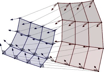
Figure 1. Bäcklund mates

The last condition in Definition 3 could be replaced by the requirement that the connecting line $p_{i}\vee q_{i}$ is perpendicular to both normal vectors, $\mathbf{n}_{i}$ and $\mathbf{m}_{i}$.

In the classical theory, Bäcklund transforms of smooth surfaces $\Phi$, $\Psi$ can be defined by the same three conditions as in Definition 3 (with the understanding that both surfaces are parametrized over the same domain and corresponding points, normals, and tangent planes belong to the same parameter values). It is our aim in this article to prove several results on Bäcklund transforms of principal contact element nets that are also valid in the smooth theory and in other discrete settings. The most important property states that only pseudospheres admit Bäcklund transforms.

Theorem 4.

If a principal contact element net $(p,\mathbf{n})$ admits a Bäcklund transform, it is of constant negative Gaussian curvature

(1) $$K=-\frac{\sin^{2}\varphi}{d}$$

where $d$ is the distance between corresponding points and $\varphi$ is the angle between corresponding normals.

We still have to explain the notion of Gaussian curvature to which this theorem refers. In the smooth setting, the Gaussian curvature in a point can be defined as the local area distortion under the Gauss map. This is imitated in

Definition 5.

The Gaussian curvature $K$ of an elementary quadrilateral $(p_{0},\mathbf{n}_{0})$, $(p_{1},\mathbf{n}_{1})$, $(p_{2},\mathbf{n}_{2})$, $(p_{3},\mathbf{n}_{3})$ of a principal contact element net is defined as

(2) $$K=\frac{S_{0}}{S}$$

where $S_{0}$ is the oriented area of the spherical quadrilateral $\mathbf{n}_{0}$, $\mathbf{n}_{1}$, $\mathbf{n}_{2}$, $\mathbf{n}_{3}$ and $S$ is the oriented area of the circular quadrilateral $p_{0}$, $p_{1}$, $p_{2}$, $p_{3}$.

The Gaussian curvature as defined here is a well-accepted concept in discrete differential geometry (see [4]) and it is a special case of a recently published and more general theory [5]. Note that in contrast to the smooth setting, the Gaussian curvature is assigned to a face and not to a vertex. This allows us to speak of the Gaussian curvature of an elementary quadrilateral.

It will be convenient to speak of the twist of two oriented lines and also of the twist of Bäcklund mates.

Definition 6.

The twist of two oriented lines $N$ and $M$ is defined as the ratio

(3) $$\operatorname*{twist}(N,M)=\frac{\sin\varphi}{d}$$

where $\varphi$ is the angle between the respective direction vectors $\mathbf{n}$ and $\mathbf{m}$ (measured according to the convention of Definition 3) and $d$ is the distance between $N$ and $D$ (Figure 2). The twist of two Bäcklund mates is defined as the twist of any two corresponding normal lines.

Figure 2. Transversals of four relative revolute axes

We will argue that Theorem 4 is a consequence of the Theorem 8, below, which deserves interest in its own. In order to formulate this result, we recall a definition from [13]:

Definition 7.

A cyclic sequence $A_{0}$, $A_{1}$, $A_{2}$, $A_{3}$ of direct Euclidean displacements $A_{i}\colon E^{3}\to E^{3}$ is called a rotation quadrilateral, if any two neighboring positions correspond in a rotation.

A generic rotation quadrilateral has four relative revolute axes $K_{01}$, $K_{12}$, $K_{23}$, $K_{30}$ (in the moving space) that admit two transversal lines $N$ and $M$. Denote the feet of their common perpendicular by $p\in N$ and $q\in M$ and one of their unit direction vectors by $\mathbf{n}$ and $\mathbf{m}$ (thus imposing an orientation on $N$ and $M$). It was shown in [13] that precisely the homologous images of the two contact elements $(p,\mathbf{n})$ and $(q,\mathbf{m})$ can serve as corresponding elementary quadrilaterals of Bäcklund mates. This leads us to an important result that relates the Bäcklund transform of pseudospherical principal contact element nets to discrete rotating motions.

Theorem 8.

Consider a rotation quadrilateral $A_{0}$, $A_{1}$, $A_{2}$, $A_{3}$ with relative revolute axes $K_{01}$, $K_{12}$, $K_{23}$, $K_{30}$ in the moving space. Denote by $N$ and $M$ their transversals, by $\mathbf{n}$ and $\mathbf{m}$ one of their respective unit direction vectors and by $p\in N$ and $q\in M$ the feet of their common normals (Figure 2). Then the Gaussian curvature of the homologous images of $(p,\mathbf{n})$ and $(q,\mathbf{m})$ equals $-\operatorname*{twist}^{2}(N,M)$, that is, it can be computed by (1) where $d=\operatorname*{dist}(p,q)$ and $\varphi=\sphericalangle(\mathbf{n},\mathbf{m})$.

As a consequence of Theorem 8 a pseudospherical principal contact element net of Gaussian curvature $K$ admits Bäcklund transforms of twist $\pm\sqrt{-K}$.

In retrospect and especially when studying its relation to Theorem 4, the content of Theorem 8 is maybe a rather obvious conjecture. Nonetheless, it is surprising when viewed independently. There are six degrees of freedom when fitting a rotation quadrilateral to two given lines $N$ and $M$: Three choices for every relative rotation makes a total of twelve degrees of freedom; the requirement that their composition yields the identity consumes six of them. Still, this is insufficient to change the area ratio (2).

Our proof of Theorem 8 uses the dual quaternion calculus of rigid motions. It allows a computational proof that requires only linear operations. Nonetheless, the involved calculations are so complicated that assistance of a CAS seems indispensable. The reason for this is the rather involved spatial configuration and the high number of degrees of freedom. Theorems 4 and 8 will both be proved in Section 3.

A certain converse of Theorem 4 is the construction of the Bäcklund transform from a given pseudospherical principal contact element net. It is on the agenda in Section 4.

Theorem 9.

Given a pseudospherical principal contact element net $(p,\mathbf{n})$ of negative Gaussian curvature $K$ and a contact element $(q_{i},\mathbf{m}_{i})$ such that

• $q_{i}$ lies in the tangent plane $\pi_{i}$ of $p_{i}$,

• $\mathbf{m}_{i}$ is perpendicular to the line $p_{i}\vee q_{i}$, and

• the quantities $K$, $d=\operatorname*{dist}(p_{i},q_{i})$ and $\varphi=\sphericalangle(\mathbf{n}_{i},\mathbf{m}_{i})$ satisfy (1)

there exists precisely one Bäcklund transform $(q,\mathbf{m})$ of $(p,\mathbf{n})$ such that $(p_{i},\mathbf{n}_{i})$ and $(q_{i},\mathbf{m}_{i})$ correspond.

As we will see, there exists a simple necessary construction for the neighbours of the contact element $(q_{i},\mathbf{m}_{i})$. This already implies uniqueness of the Bäcklund transform. In order to prove existence, we have to show that the conditions on $q_{i}$ and $\mathbf{m}_{i}$ imply that this construction does not lead to contradictions. The proof consists once more of a direct CAS-aided computation.

One interpretation of Theorem 9 is that every pseudospherical principal contact element net can be generated in infinitely many ways as trajectory of a discrete rotating motion that has a second, non-parallel trajectory surface of the same type. Combining this observation with results of [12], in particular with [12, Theorem 7], we get an interesting corollary (the terminology is explained in the standard reference [4] on discrete differential geometry):

Corollary 10.

Principal contact element nets of a prescribed negative Gaussian curvature are described by a multidimensionally consistent $2D$-system.

This corollary certainly admits simple direct proofs. Still, we are not aware of a reference that actually states it.

We should also mention that our results are in perfect analogy to the smooth setting. If $\Phi$ and $\Psi$ are Bäcklund mates, the correspondence between their points can be realized by principal parametrizations $\mathbf{x}(u,v)$ and $\mathbf{y}(u,v)$. For every parameter pair $(u,v)$, we obtain a rigid figure consisting of corresponding points $\mathbf{x}(u,v)$, $\mathbf{y}(u,v)$ and the respective surface normals. This induces a two-parametric motion $A(u,v)$ with the following properties:

• $A(u,v)$ is a gliding motion on both surfaces $\Phi$ and $\Psi$ [8, Section 7.1.5]. This means that there exist two planes in the moving space whose images under $A(u,v)$ envelop $\Phi$ and $\Psi$, respectively.

• The infinitesimal motions in $u$- and $v$-parameter directions are infinitesimal rotations. (This is a general property of gliding motions along principally parametrized surfaces.)

In our discrete setting, both properties are preserved. The infinitesimal rotations of the continuous case are replaced by rotations between finitely separated positions.

Our final result, which will be presented in more detail in Section 5, is Bianchi’s Permutation Theorem for Bäcklund transforms of pseudospherical principal contact element nets:

Theorem 11.

Suppose $(b,\mathbf{l})$ and $(c,\mathbf{m})$ are two Bäcklund transforms of the same twist to a principal contact element net $(a,\mathbf{k})$. Then there exists a unique principal contact element net $(d,\mathbf{n})$ which is at the same time a Bäcklund transform of $(b,\mathbf{l})$ and $(c,\mathbf{m})$.

Note that throughout this article we implicitely make a number of assumptions on the genericity of the involved geometric entities. More specifically, we require that the Gaussian curvature (2) is well-defined for all elementary quadrilaterals of principal contact element nets (with the notable exception of Example 15. The meaning of the word “generic” in the paragraph folling Definition 7 is not as easily explained. We require that indeed two transversals to the four relative revolute axes exist in algebraic sense. This can be formulated as a non-vanishing condition of an algebraic expression in the input paramters. Moreover, neighbouring relative revolute axes are assumed to be skew.

3. The Gaussian curvature of Bäcklund mates

This section is dedicated to the proof of Theorem 4. Assume that $(p,\mathbf{n})$ and $(q,\mathbf{m})$ are Bäcklund mates, denote the distance of corresponding points by $d$ and the angle of corresponding normals by $\varphi$. We want to show that the Gaussian curvature of all elementary quadrilaterals of $(p,\mathbf{n})$ is constant and can be computed by (1).

Our first observation concerns two neighbouring pairs of corresponding contact elements.

Lemma 12.

Under the conditions of Theorem 4, any two neighbouring pairs $(p_{0},\mathbf{n}_{0})$, $(p_{1},\mathbf{n}_{1})$ and $(q_{0},\mathbf{m}_{0})$, $(q_{1},\mathbf{m}_{1})$ of corresponding contact elements correspond in a rotation $R_{01}$ about the line $L_{01}=h_{01}\vee k_{01}$ where $h_{01}=N_{0}\cap N_{1}$ and $k_{01}=M_{0}\cap M_{1}$.

Proof.

By Definition 3, the figures formed by corresponding contact elements are congruent and of equal orientation. Thus, there exists a direct Euclidean displacement $R_{01}$ such that $R_{01}(p_{0},\mathbf{n}_{0})=(p_{1},\mathbf{n}_{1})$ and $R_{01}(q_{0},\mathbf{m}_{0})=(q_{1},\mathbf{m}_{1})$. By Definition 2 the points $h_{01}$ and $k_{01}$ are fix-points of $R_{01}$. Thus, $R_{01}$ is indeed a rotation about the line $L_{01}$. ∎

Consider now corresponding elementary quadrilaterals $(p_{0},\mathbf{n}_{0})$, …, $(p_{3},\mathbf{n}_{3})$, and $(q_{0},\mathbf{m}_{0})$, …, $(q_{3},\mathbf{m}_{3})$ of the two Bäcklund mates. They define four relative rotations $R_{01}$, $R_{12}$, $R_{23}$, $R_{30}$ such that

(4) $$R_{30}\circ R_{23}\circ R_{12}\circ R_{01}=\mathrm{id.}$$

This observation relates the Bäcklund transform of pseudospherical principal contact element nets to the geometry of rotation quadrilaterals [13] and discrete gliding motions [12]. We will use results and techniques from both articles for our proof.

More specifically, we view each figure $(p_{i},\mathbf{n}_{i})$, $(q_{i},\mathbf{m}_{i})$ as the position of a rigid body in space. This gives us four direct Euclidean displacements

(5) $$A_{i}\colon E^{3}\to E^{3}$$

from the moving space $E^{3}$ to an identical copy of $E^{3}$, the fixed space. They form a rotation quadrilateral in the sense of Definition 7. Theorem 8 states that the Gaussian curvature of an elementary quadrilateral depends only on the relative position of two corresponding normal lines. Since this is the same for all elementary quadrilaterals, Theorem 4 follows.

In our proof of Theorem 8 we use the dual quaternion calculus of spatial kinematics. It is explained for example in [7]. A short primer is also given in [12]. We use the notation of the latter article. A direct Euclidean displacement is modelled as a unit dual quaternion $A=\hat{A}+\varepsilon\tilde{A}$ where $\hat{A}$ and $\tilde{A}$ are its respective primal and dual part and $\varepsilon$ satisifes $\varepsilon^{2}=0$. Assembling the components of primal and dual parts into a homogeneous vector $[\hat{A},\tilde{A}]=[a_{0},\ldots,a_{7}]$, we can view $A$ as a point on the

(6) $$\mathcal{S}\subset P^{7}\colon\hat{A}\cdot\tilde{A}=0.$$

This quadric is called the Study quadric.

Proof of Theorem 8.

We start by setting up a system of equations that describe a rotation quadrilateral whose relative rotation axes in the moving space intersect two fixed lines $N$ and $M$. At first, we specify the two lines $N$ and $M$ in the moving space. Without loss of generality, the normal feet $p$ and $q$ on $N$ and $M$, respectively, can be chosen as

(7) $$p=(0,0,e),\quad q=(0,0,-e)$$

where $2e=d$. The respective directions vectors of $N$ and $M$ are

(8) $$\mathbf{n}=(1,t,0),\quad\mathbf{m}=(1,-t,0)$$

where $t$ is related to the angle $\varphi$ between $N$ and $M$ via $\varphi=2\arctan t$. Note that the vectors $\mathbf{n}$ and $\mathbf{m}$ are not normalized so that we ultimately will not compute the Gaussian image of an elementary quadrilateral on the unit sphere but on a sphere of squared radius $1+t^{2}$. This is admissible since the Gaussian curvature will only be multiplied by the constant factor $1+t^{2}$.

Without loss of generality, the first position of the rotation quadrilateral can be taken as the identity, $A_{0}=[1,0,\ldots,0]$ (we use homogeneous coordinates in $P^{7}$). The two neighbouring positions are

(9) $$A_{1}=[a_{10},\ldots,a_{17}],\quad\text{and}\quad A_{3}=[a_{30},\ldots,a_{37}].$$

Their components $a_{ij}$ are subjects to seven constraints:

• The relative displacements $R_{01}$ and $R_{03}$ are rotations. In the dual quaternion calculus this constraint is modelled as

  (10) $$\pi_{5}(A_{i}\star A_{0}^{-1})=0,\quad i\in\{1,3\},$$

  where $\pi_{5}$ denotes the projection onto the fifth coordinate.

• The relative revolute axes $K_{01}$ and $K_{03}$ intersect $M$ and $N$:

  (11) $$\Omega({(R_{0i})}_{\varepsilon}\star\mathfrak{v}{{(R_{0i}\star A_{0})}_{\varepsilon}}\star{(R_{0i}^{-1})}_{\varepsilon},T)=0;\quad i\in\{1,3\},\ T\in\{M,N\}.$$

  In this equation, $\Omega$ is the bilinear form associated to the Study quadric ($\Omega(X,Y)=\hat{X}\cdot\tilde{Y}$), the subscript $\varepsilon$ denotes $\varepsilon$-conjugation of dual quaternions, and $\mathfrak{v}{X}$ is the vector part of the dual quaternion $X$.

• The sought positions lie on the Study quadric $\mathcal{S}$:

  (12) $$\Omega(A,A)=\hat{A}_{i}\cdot\tilde{A}_{i}=0,\quad i\in\{1,3\}.$$

Equations (10) and (11) are linear in the components of $A_{1}$ and $A_{3}$, Equation (12) is quadratic. Normalizing by $a_{10}=ta_{13}$, the general solution for $A_{1}$ reads

(13) $$\begin{gathered}A_{1}=(ta_{13},ta_{11}a_{13},ta_{13}^{2},0,-t^{2}a_{11}a_{13},a_{12}a_{13},t^{2}a_{11}^{2}-a_{12}^{2});\\ a_{11},a_{12},a_{13}\in\mathbb{R}.\end{gathered}$$

Here, $a_{11}$, $a_{12}$, and $a_{13}$ serve as free parameters. The solution for $A_{3}$ is obtained by replacing the parameter $a_{1j}$ with $a_{3j}$ ($j=1,2,3$).

Similarly, the missing position $A_{2}$ is uniquely determined by two linear equations $E_{1}$, $E_{2}$ of type (10), four linear equation $E_{3}$, …, $E_{6}$ of type (11) and one quadratic equation $E_{7}$ of type (12). Thus, it is the second intersection point of a straight line through $A_{0}$ with the Study quadric $\mathcal{S}$. The solution is unique and can be computed in rational arithmetic.

While it is possible to compute $A_{2}$ and verify (1) directly, the involved expressions are excessively long. Our implementation of this approach delivers the desired result but only after a few hours of computation. Therefore, we favor a method which is based on ideal theory and yields a confirmatory answer within a few minutes. The basic idea is to show that a certain polynomial (Equation (18), below) is contained in the ideal spanned by the polynomial equations $E_{1}$, …, $E_{7}$.

For $i\in\{0,1,2,3\}$ we compute the images $p_{i}$ of the normal foot $p$ and the images $\mathbf{n}_{i}$ of the direction vector $\mathbf{n}$ under the displacement $A_{i}$ (with the entries $a_{2i}$ of $A_{2}$ left unspecified). This can be accomplished by using the following formulas for the action of a dual quaternion $A$ on a homogeneous coordinate vector $[x_{0},x_{1},x_{2},x_{3}]=[x_{0},\mathbf{x}]$:

(14) $$x^{\prime}_{0}+\varepsilon\mathbf{x}^{\prime}={A}_{\varepsilon}\star(x_{0}+\varepsilon\mathbf{x})\star\bar{A}$$

(the bar denotes dual quaternion conjugation). Note that the use of homogeneous coordinates avoids the introduction of denominators — this is highly desirable in CAS calculations of a large complexity — but has to be taken into account later in (15) when computing oriented areas.

Instead of computing the oriented area of the quadrilaterals $p_{0}$, $p_{1}$, $p_{2}$, $p_{3}$ and $\mathbf{n}_{0}$, $\mathbf{n}_{1}$, $\mathbf{n}_{2}$, $\mathbf{n}_{3}$ we compute the areas $S$ and $S_{0}$ of their respective projection onto the first and second coordinate. This is possible since an orthographic projection does not affect the ratio of areas in parallel planes. We have

(15) $$\begin{gathered}S=\sum_{i=0}^{3}(p_{i,1}p_{i+1,2}-p_{i,2}p_{i+1,1})\varkappa_{i+2}\varkappa_{i+3},\\ S_{0}=\sum_{i=0}^{3}(\mathbf{n}_{i,1}\mathbf{n}_{i+1,2}-\mathbf{n}_{i,2}\mathbf{n}_{i+1,1})\varkappa_{i+2}\varkappa_{i+3}\end{gathered}$$

(indices modulo four). The factors $\varkappa_{i}=\sum_{j=0}^{3}a_{ij}^{2}$ compensate the use of homogeneous coordinates in the computation of the points $p_{i}$ and the ideal points (vectors) $\mathbf{n}_{i}$. Now we have to show that

(16) $$\frac{S_{0}}{S}=-\frac{t^{2}}{(1+t^{2})e^{2}},$$

or, equivalently,

(17) $$(1+t^{2})e^{2}S_{0}-t^{2}S=0.$$

Equation 17 is polynomial. It holds true if its left-hand side is contained in the ideal $J$ spanned by the seven equations $E_{1}$, …, $E_{7}$ that determine the fourth position of $A_{2}$. The indeterminates are $a_{20}$, …, $a_{27}$ while $a_{11}$, $a_{12}$, $a_{13}$, $a_{31}$, $a_{32}$, $a_{33}$, $e$, $t$ serve as parameters. We perform the necessary algebraic manipulations by means of the CAS Maple 13 and assume that the defining equations of $A_{2}$ are stored in E1, …, E7. Moreover, the simplifying normalization $a_{20}=1$ is applied.

1with(Groebner):2# J defined by linear and quadratic equations3J := [E1, E2, E3, E4, E5, E6, E7]:45# Use tdeg term order:6TO := tdeg(a21, a22, a23, a24, a25, a26, a27):78# Interreduce J and reduce R with respect to this reduced ideal.9# The result is indeed 0, showing that R is contained in J.10J := InterReduce(J, TO):11Reduce([R], J, TO)[1];The final output is $0$, showing that R is indeed contained in the ideal J. ∎

This proof also finishes the proof of Theorem 4. A few explaining remarks concerning the computer calculation seem appropriate:

• The tdeg-term ordering (Line 6) is primarily by total degree and then reversed lexicographic.

• Inter-reducing the generating elements of the ideal J with respect to the term order TO (Line 10) produces a list of polynomials that generate the same ideal J but are reduced in the sense that no monomial is reducible by the leading monomial of another list element.

• The command Reduce (Line 11) computes the remainder of R divided by the polynomials in J. Its vanishing implies that R is indeed contained in the ideal spanned by J.

The running time of this implementation is approximately six minutes. Minor improvements are possibly by adapting the order of the variables in Line 6. We regret not being able to offer a proof of Theorem 4 that does not rely on a computer algebra system. The main reason for the computational difficulties (in spite of the fact that the problem is linear) is the high number of six free parameters. A more insightful proof or a proof with manually tractable calculations would be desirable.

4. Construction of the Bäcklund transform

In this section we provide an algorithm for actually constructing (or computing) the Bäcklund transforms of a pseudospherical principal contact element net. The proof of correctness of this algorithm is at the same time the proof of Theorem 9.

It is a simple observation that the Bäcklund transform $(q,\mathbf{m})$ in Theorem 9 is necessarily unique. Existence is a different matter. Given the principal contact element net $(p,\mathbf{n})$ and the contact element $(q_{i},\mathbf{m}_{i})$, any neighbour $(q_{j},\mathbf{m}_{j})$ to $(q_{i},\mathbf{m}_{i})$ is uniquely determined. It is found by the following steps whose necessity has already been discussed:

• Determine the points $h_{ij}=N_{i}\cap N_{j}$ and $k_{ij}=M_{i}\cap\beta_{ij}$ where $\beta_{ij}$ is the bisector plane of $p_{i}$ and $p_{j}$.

• Determine the unique rotation $R_{ij}$ about the axis $L_{ij}=h_{ij}\vee k_{ij}$ that transforms $(p_{i},\mathbf{n}_{i})$ into $(p_{j},\mathbf{n}_{j})$.

• The contact element $(q_{j},\mathbf{m}_{j})$ is the image of $(q_{i},\mathbf{m}_{i})$ under the rotation $R_{ij}$.

We refer to this construction briefly as the “neighbour construction”. Note that a minor variation takes as input the oriented lines $N_{i}$, $N_{j}$ and $M_{i}$ (as opposed to three contact elements) and returns the oriented line $M_{j}$.

We provide some more information on the actual computation of the neighbour construction — not only as a service for the reader but also because we need them later in the proof of Lemma 13 and Theorem 9.

Throughout this calculation we use homogeneous coordinates to describe points and planes, Plücker coordinates to describe lines and homogeneous four by four matrices to describe Euclidean displacements. (Here, the use of dual quaternion calculus does not provide a significant advantage.) The bisector plane $\beta$ of two non-ideal points $[x_{0},x_{1},x_{2},x_{3}]=[x_{0},\mathbf{x}]$ and $[y_{0},y_{1},y_{2},y_{3}]=[y_{0},\mathbf{y}]$ has homogeneous coordinates

(18) $$[y_{0}^{2}\;\mathbf{x}\cdot\mathbf{x}-x_{0}^{2}\;\mathbf{y}\cdot\mathbf{y},2x_{0}y_{0}\;\mathbf{x}\times\mathbf{y}].$$

The intersection point of the plane $[u_{0},u_{1},u_{2},u_{3}]=[u_{0},\mathbf{u}]$ and the line with Plücker coordinates $[g_{1},g_{2},g_{3},h_{1},h_{2},h_{3}]=[\mathbf{g},\mathbf{h}]$ equals

(19) $$[x_{0},\mathbf{x}]=[\mathbf{u}\cdot\mathbf{g},-u_{0}\mathbf{g}+\mathbf{u}\times\mathbf{h}].$$

Because of $h_{ij}=N_{i}\cap\beta_{ij}=N_{j}\cap\beta_{ij}$ this formula can be used to determine both, $k_{ij}$ and $h_{ij}$.

The rotation $R_{ij}$ can be conveniently written as the composition of two reflections in the bisector plane $\beta_{ij}$ and the plane $\gamma_{ij}=p_{j}\vee h_{ij}\vee k_{ij}$. This is true since the composition of two reflections in planes $\beta$ and $\gamma$ is a rotation about the intersection line $L=\beta\cap\gamma$. Moreover, it is obvious that $(p_{i},\mathbf{n}_{i})$ is transformed into $(p_{j},\mathbf{n}_{j})$. The homogeneous transformation matrix $[R_{ij}]$ of $R_{ij}$ is given by

(20) $$[R_{ij}]=[C_{ij}]\cdot[B_{ij}]$$

where $[B_{ij}]$ and $[C_{ij}]$ are the reflection matrices in $\beta_{ij}$ and $\gamma_{ij}$, respectively. They can be computed by means of the general formula for the reflection matrix in a plane $[u_{0},u_{1},u_{2},u_{3}]$ which reads

(21) $$\begin{bmatrix}u_{1}^{2}+u_{2}^{2}+u_{3}^{2}&0&0&0\\ -2u_{0}u_{1}&-u_{1}^{2}+u_{2}^{2}+u_{3}^{2}&-2u_{1}u_{2}&-2u_{1}u_{3}\\ -2u_{0}u_{2}&-2u_{1}u_{2}&u_{1}^{2}-u_{2}^{2}+u_{3}^{2}&-2u_{2}u_{3}\\ -2u_{0}u_{3}&-2u_{1}u_{3}&-2u_{2}u_{3}&u_{1}^{2}+u_{2}^{2}-u_{3}^{2}\end{bmatrix}.$$

Equations (18)–(21) are sufficient for a CAS implementation of the neighbour construction.

We return to the proof of Theorem 9 where existence is still open. The problem with the neighbour construction is that it will produce contradictions for a general choice of $(q_{0},\mathbf{m}_{0})$. Consider only an elementary quadrilateral $(p_{0},\mathbf{n}_{0})$, …, $(p_{3},\mathbf{n}_{3})$ and the contact element $(q_{0},\mathbf{m}_{0})$. By the neighbour construction we obtain (in that order) the contact elements $(q_{1},\mathbf{m}_{1})$, $(q_{2},\mathbf{m}_{2})$, and $(q_{3},\mathbf{m}_{3})$. Applying the neighbour construction once more, we get a contact element $(q^{\star}_{0},\mathbf{m}^{\star}_{0})$ which should equal $(q_{0},\mathbf{m}_{0})$.

Since the Gaussian curvature $K$ and the distance $d$ between corresponding points is already defined, we necessarily have to choose $\mathbf{m}_{0}$ so that the angle $\varphi=\sphericalangle(\mathbf{n}_{0},\mathbf{m}_{0})$ satisfies (1). Thus, there are only four choices for the unit vector $\mathbf{m}_{0}$ and only two choices for the normal line $M_{0}$. We will show that all of them lead to valid solutions. This is also enough to ensure that the neighbour construction can be consistently applied to the whole principal contact element net. The proof of this still needs some preparatory work.

To begin with, we mention those configuration that will be identified as false positives by our test $(q_{0},\mathbf{m}_{0})=(q^{\prime}_{0},\mathbf{m}^{\prime}_{0})$.

• If $M_{0}$ intersects the axis of the circle through $p_{0}$, $p_{1}$, $p_{2}$, $p_{3}$, the composition of the four rotations yields the identity but the homologous contact elements $(q_{0},\mathbf{m}_{0})$, …, $(q_{3},\mathbf{m}_{3})$ do not form the elementary quadrilateral of a principal contact element net.

• If $M_{0}$ is parallel to $N_{0}$ the action of the rotation $R_{i,i+1}$ on $(q_{i},\mathbf{m}_{i})$ equals that of the reflection in $\beta_{i,i+1}$. Therefore, we get $(q^{\star}_{0},\mathbf{m}^{\star}_{0})=(q_{0},\mathbf{m}_{0})$ also in this case. The Gaussian curvature of the two elementary quadrilaterals is, however, different.

It goes without saying that both configurations violate the pre-requisites of Theorem 8.

The following lemma states that the neighbour construction acts projectively on the set of lines obtained by revolving $M_{0}$ about $N_{0}$. It allows a simplifying assumption during the later calculations.

Lemma 13.

Consider three lines $N_{0}$, $N_{1}$ and $M_{0}$ such that $M_{0}$ and $N_{0}$ are skew while $N_{0}$ and $N_{1}$ are intersecting. Denote the set of lines obtained by rotating $M_{0}$ about $N_{0}$ by $\mathcal{M}_{0}$. Then the neighbour construction with respect to $N_{0}$ and $N_{1}$ (equipped with some orientation) induces a projective mapping between $\mathcal{M}_{0}$ and its image $\mathcal{M}_{1}$ under the neighbour construction. (Figure 3).

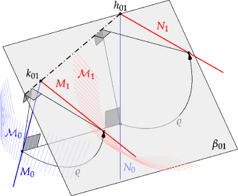
Figure 3. Notation in Lemma 13

Proof.

Our computation is based on a Cartesian coordinate frame $\{o;x,y,z\}$ which is projectively extended such that vanishing of the first coordinate characterizes ideal points. We choose $N_{0}$ as the $z$-axis and $M_{0}$ such that the shortest distance between $N_{0}$ and $M_{0}$ is attained at the pedal points $[1,0,0,0]\in N_{0}$ and $[1,1,0,0]\in M_{0}$. The ideal point on $M_{0}$ than equals $[0,0,1,v]$ with some $v\in\mathbb{R}$. Because of the rotational symmetry of the set $\mathcal{M}_{0}$, we may assign the coordinates $[s,0,t,u]$ to the bisector plane $\beta_{01}$ of $N_{0}$ and $N_{1}$. Identifying geometric entities with their homogeneous coordinate vectors, we can write

(22) $$\begin{gathered}N_{0}=[0,0,1,0,0,0],\ N_{1}=[0,2tu,u^{2}-t^{2},2st,0,0],\\ h_{01}=N_{0}\cap\beta_{01}=N_{0}\cap N_{1}=[u,0,0,-s],\\ M_{0}(\lambda)=[-2\lambda,\lambda^{2}-1,u(\lambda^{2}+1),2u\lambda,u(1-\lambda^{2}),1+\lambda^{2}].\end{gathered}$$

As expected, $M_{0}(\lambda)$ is a quadratic parametrization in Plücker coordinates of the line-set $\mathcal{M}_{0}$. The theorem’s statement amounts to saying that $M_{1}(\lambda)$ is also quadratic. The intersection point of $M_{0}$ with $\beta_{01}$ equals

(23) $$k_{01}(\lambda)=\begin{bmatrix}uv-t+(t+uv)\lambda^{2}\\ t-uv+2s\lambda+(t+uv)\lambda^{2}\\ s+2uv\lambda-s\lambda^{2}\\ -sv-2tv\lambda-sv\lambda^{2}\end{bmatrix}.$$

Now we compute $M_{1}(\lambda)$ by reflecting $M_{0}(\lambda)$, at first in the plane $\beta_{01}$ and then in $\gamma_{01}=N_{1}\vee k_{01}(\lambda)$. We refrain from giving the details of the calculation; the relevant formulas are (18)–(21). The outcome is a polynomial vector function $M_{1}(\lambda)$ which a priory is of degree 20 in $\lambda$. However, all of its entries have the common factor

(24) $$(t^{2}+u^{2})^{9}(1+\lambda^{2})^{8}G(\lambda)$$

with the quadratic polynomial

(25) $$G(\lambda)=s^{2}+t^{2}-2tuv+u^{2}v^{2}+4st\lambda+(s^{2}+t^{2}+2tuv+u^{2}v^{2})\lambda^{2}.$$

This common factor (24) can be split off so that only a quadratic component remains. ∎

Remark 14.

The vanishing of the polynomial (24) has a geometric meaning.

• If $t^{2}+u^{2}$ vanishes, the plane $\beta_{01}$ is at infinity and the reflection in $\beta_{01}$ becomes undefined.

• If $1+\lambda^{2}$ vanishes, the direction of the revolute axis $\beta_{01}\cap\gamma_{01}$ is isotropic and the rotation becomes singular. The same is true for the zeros of $G(\lambda)$.

All of these instances are irrelevant in our setting.

Lemma 13 implies that the map

(26) $$\eta\colon\mathcal{M}_{0}\to\mathcal{M}_{0},\quad M_{0}\mapsto M^{\star}_{0},$$

as a composition of neighbour maps, is projective as well. The line-set $\mathcal{M}_{0}$ is of course the set obtained by subjecting $M_{0}$ to all rotations about $N_{0}$. We conclude that $\eta$ generically has two fixed lines — those lines of $\mathcal{M}_{0}$ that intersect the $z$-axis. We are interested in configurations where a non-trivial fixed line $M_{0}\in\mathcal{M}_{0}$ exists. In this case $\eta$ is the identity on $\mathcal{M}$. This can also be phrased as follows: If $(q_{0},\mathbf{m}_{0})$ is such that the neighbour construction is free of contradictions, the same is true for every contact element that is obtained from $(q_{0},\mathbf{m}_{0})$ by a rotation about $N_{0}$. This observation gives us one extra degree of freedom for a simplifying assumption in the

Proof of Theorem 9.

The basic idea is to show that in the pencil of lines $M_{0}$ incident with $q_{0}$ and perpendicular to $p_{0}\vee q_{0}$ precisely two lines result in a closed chain of neighbouring contact elements obtained by successive application of the neighbour construction. These solutions necessarily satisfy the condition of the theorem.

We begin by assigning homogeneous coordinates to the four points $p_{0}$, $p_{1}$, $p_{2}$, $p_{3}$. Without loss of generality we may set

(27) $$p_{i}=[1+t_{i}^{2},1-t_{i}^{2},2t_{i},0],\quad i=0,\ldots,3.$$

The values $t_{i}$ are in $\mathbb{R}\cup\{\infty\}$ and $t_{i}=\infty$ corresponds to the point $[1,-1,0,0]$. The following calculations do not take into account this exceptional value but could easily be adapted to handle this situation. Moreover, we make the admissible simplification $t_{0}=0$.

The bisector planes of the points $p_{i}$ and $p_{j}$ are

(28) $$\beta_{ij}=[0,S_{ij},T_{ij},0],\quad i,j=0,\ldots,3;\ i\neq j$$

where $S_{ij}=t_{i}+t_{j}$ and $T_{ij}=t_{i}t_{j}-1$. The reflection in $\beta_{ij}$ is described by the matrix

(29) $$[B_{ij}]\begin{bmatrix}S_{ij}^{2}+T_{ij}^{2}&0&0&0\\ 0&T_{ij}^{2}-S_{ij}^{2}&-2S_{ij}T_{ij}&0\\ 0&-2S_{ij}T_{ij}&S_{ij}^{2}-T_{ij}^{2}&0\\ 0&0&0&S_{ij}^{2}+T_{ij}^{2}\end{bmatrix}.$$

Starting with the normal vector $\mathbf{n}_{0}=[0,u,v,1]$, we compute

(30) $$\mathbf{n}_{1}=[B_{01}]\cdot\mathbf{n}_{0},\quad\mathbf{n}_{3}=[B_{30}]\cdot\mathbf{n}_{0},\quad\mathbf{n}_{2}=[B_{21}]\cdot\mathbf{n}_{1}.$$

The first point $q_{0}$ of the Bäcklund transform should be such that the connecting line $p_{0}\vee q_{0}$ is perpendicular to $\mathbf{n}_{0}$. Due to Lemma 13, the possible choices for $\mathbf{m}_{0}$ can be parametrized as

(31) $$\mathbf{m}_{0}=[0,\lambda u,\lambda v,ev+\lambda].$$

Note that the invalid choice $\mathbf{m}_{0}\parallel\mathbf{n}_{0}$ corresponds to $\lambda\to\infty$ and will automatically drop out during our calculations. The second invalid choice is obtained for $\lambda=0$ in which case the line $M_{0}$ intersects the circle axis.

The point $q_{0}$ is then

(32) $$q_{0}=[1+t_{0}^{2},1-t_{0}^{2}+ev,2t_{0}-eu,0]$$

where $e$ is a parameter that determines the distance between $p_{0}$ and $q_{0}$.

Using the additional admissible simplification $t_{0}=0$, the intersection point $k_{0j}=M_{0}\cap\beta_{01}$ becomes

(33) $$k_{0j}=\begin{bmatrix}(ut_{1}-v)\lambda\\ -(v+e(u^{2}+v^{2}))\lambda\\ -(v+e(u^{2}+v^{2}))t_{1}\lambda\\ -(t_{1}+t_{1}e(u+v))(ev+\lambda)\end{bmatrix},\quad j\in\{1,3\}.$$

By means of (20) and (21), we compute the rotations $R_{01}$ and $R_{03}$ to obtain the homogeneous coordinates of the points $q_{1}$, $q_{3}$ and the vectors (ideal points) $\mathbf{m}_{1}$, $\mathbf{m}_{3}$. Common factors of the shape

(34) $$e^{2}(u^{2}+v^{2})(1+t_{j}^{2})^{4},\quad j\in\{1,3\},$$

can be split off. The resulting expressions are just a little too long to be displayed here.

In the same way, we compute the intersection points $k_{12}$ and $k_{23}$, where we immediately split off the common factor

(35) $$(1+t_{j}^{2})^{2}((u^{2}+v^{2}+1)(ut_{j}-v)^{2}\lambda^{2}+v^{2}(eu+t_{j}(ev+1))^{2}),\quad j\in\{1,3\},$$

the rotation $R_{12}$, and the vector $\mathbf{m}_{2}$. This latter vector can be divided by $e^{2}(u^{2}+v^{2})(1+t_{1}^{2})^{6}(1+t_{2}^{2})^{4}Q(\lambda)$ where

(36) $$Q(\lambda)=(u^{2}+v^{2}+1)^{2}(t_{1}u-v)^{4}\lambda^{4}+\\ 2v^{2}(eu+t_{1}(ev+1))^{2}(u^{2}+v^{2}+1)(t_{1}u-v)^{2}\lambda^{2}+v^{4}(eu+t_{1}(ev+1))^{4}.$$

The closure condition of the neighbor construction is now the linear dependence of $\mathbf{m}_{2}$ and the ideal point (direction vector) $[0,\mathbf{k}_{2}]$ of $k_{12}\vee k_{23}$. It turns out that $\mathbf{k}_{2}$ can be divided by

(37) $$(t_{1}-t_{3})(v+e(u^{2}+v^{2}))\lambda.$$

We compute the cross-product $\mathbf{m}_{2}\times\mathbf{k}_{2}$ and extract the greatest common divisor

(38) $$2evt_{2}G_{1}(\lambda)G_{2}(\lambda)$$

of its entries. Here, $G_{1}(\lambda)$ and $G_{2}(\lambda)$ are quadratic polynomials in $\lambda$.

One of them, say $G_{1}$, equals $\lambda^{-1}$ times the homogenizing coordinate of $k_{12}$. It is a spurious solution since it vanishes in configurations where $\mathbf{k}_{2}$ and $\mathbf{m}_{2}$ are parallel but $M_{2}$ is different from $k_{12}\vee k_{23}$. The second factor equals

(39) $$G_{2}=v^{2}(T_{3}(e^{2}u^{2}+1-e^{2}v^{2})-2T_{2}e^{2}uv)++2ev(T_{3}(u^{2}-v^{2})-2T_{2}uv)\lambda\\ +(T_{3}(u^{2}-v^{2})-2uvT_{2})(v^{2}+u^{2}+1)\lambda^{2}$$

where

(40) $$T_{2}=t_{1}t_{2}-t_{1}t_{3}+t_{2}t_{3}+1\quad\text{and}\quad T_{3}=t_{1}t_{2}t_{3}+t_{1}-t_{2}+t_{3}.$$

Its vanishing characterizes the positions of $M_{0}$ that lead to valid solutions. Since (39) is quadratic in $\lambda$, there are precisely two solutions. This finishes the proof of Theorem 9. ∎

Example 15.

The maybe simplest example of a pair of Bäcklund mates in the continuous settings consists of a straight line $Z$, viewed as a degenerate pseudosphere, and the surface of revolution $\Psi$ obtained by rotating a tractrix with asymptote $Z$ about $Z$. We apply our construction to a discrete version of this configuration which is actually too irregular to be covered by our theory. Nonetheless, we are able to illustrate our basic ideas and to recover the geometric essence of the continuous case.

We define the first principal contact element net $(p,\mathbf{n})$ as follows:

(41) $$p\colon\mathbb{Z}^{2}\to\mathbb{R}^{3}, (i,j)\mapsto(0,0,j)$$

$$\mathbf{n}\colon\mathbb{Z}^{2}\to\mathbb{R}^{3}, \textstyle(i,j)\mapsto(0,\cos\bigl{(}\frac{2i\pi}{k}\bigr{)},\sin\bigl{(}\frac{2i\pi}{k}\bigr{)},0)$$

The integer $k\in\mathbb{N}$ is a shape parameter that affects the discretization of the revolute surface.

The principal contact element net $(p,\mathbf{n})$ is irregular in the sense that the Gaussian curvature of the elementary quadrilaterals is undefined. Nonetheless, we can construct the Bäcklund transform $(q,\mathbf{m})$ to $(p,\mathbf{n})$, defined by the contact element $(q_{0,0},\mathbf{m}_{0,0})$ with $q_{0,0}=(0,d,0)$, $\mathbf{m}_{0,0}=(0,\cos\alpha,\sin\alpha)$ and $d\in\mathbb{R}$. It is depicted in Figure 4 where we use $\alpha=\frac{\pi}{2}$.

According to our theory, the contact element $(q_{0,j+1},\mathbf{m}_{0,j+1})$ is obtained from $(p_{0,j},\mathbf{n}_{0,j})$, $(p_{0,j+1},\mathbf{n}_{0,j+1})$ and $(q_{0,j},\mathbf{m}_{0,j})$, see Figure 4, left (where we write $p_{j}$, $q_{j}$ etc. instead of $p_{0,j}$, $q_{0,j}$). It never leaves the plane $x=0$ and produces a discrete curve with vertices $q_{0,j}$ and normal vectors $\mathbf{m}_{0,j}$. The choice $\alpha=\frac{\pi}{2}$ ensures that the length of the tangent segment between $q_{0,j}$ and the $z$-axis is constant. Hence, we may address the curve as discrete tractrix.

The contact element $(q_{i+1,j},\mathbf{m}_{i+1,j})$ is constructed from the contact elements $(p_{i,j},\mathbf{n}_{i,j})$, $(p_{i+1,j},\mathbf{n}_{i+1,j})$, and $(q_{i,j},\mathbf{m}_{i,j})$. The intersection point of $M_{i,j}$ with the bisector plane of $p_{i,j}$ and $p_{i+1,j}$ is the ideal point of the $z$-axis so that $(q_{i,j},\mathbf{m}_{i,j})$ and $(q_{i+1,j},\mathbf{m}_{i+1,j})$ correspond in a rotation about the $z$-axis through the angle $\frac{2\pi}{k}$. The resulting discrete revolute surface can be seen in Figure 4, right. Its Gaussian curvature is indeed constant and negative. We refrain from deriving analytic expressions for describing this discrete surface. These have already been established in [5].

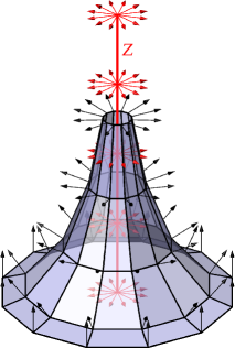
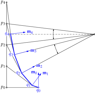
Figure 4. Discrete tractrix and pseudospherical principal contact element net of revolution

5. Bianchi’s Permutation Theorem

Now we prove Bianchi’s Permutation Theorem 11, our final major result. We split our proof into a series of intermediate steps.

Lemma 16.

Assume that $(b,\mathbf{l})$, and $(c,\mathbf{m})$ are both Bäcklund transforms of the same twist of $(a,\mathbf{k})$. If the contact elements $(b_{0},\mathbf{l}_{0})$ and $(c_{0},\mathbf{m}_{0})$ correspond to $(a_{0},\mathbf{l}_{0})$ there exists a half-turn that interchanges $(b_{0},\mathbf{l}_{0})$ and $(c_{0},\mathbf{m}_{0})$ (Figure 5).

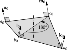
Figure 5. Opposite normals correspond in a half-turn

Proof.

In a suitable Euclidean coordinate frame, we have

(42) $$\begin{gathered}\mathbf{l}_{0}=(\cos\varphi,\sin\varphi,0),\quad\mathbf{m}_{0}=(\cos\varphi,-\sin\varphi,0),\\ b_{0}=(0,0,z)+\beta\mathbf{l}_{0},\quad c_{0}=(0,0,-z)+\gamma\mathbf{m}_{0}\end{gathered}$$

with $\varphi\in(0,\frac{\pi}{2})$ and $\beta$, $\gamma\geq 0$. We try to recover the position of $(a_{0},\mathbf{k}_{0})$. It will turn out that this is only possible, if $\beta=\gamma$, that is, $(b_{0},\mathbf{l}_{0})$ and $(c_{0},\mathbf{m}_{0})$ correspond in a half-turn.

Clearly, the possible location of $a_{0}$ is the intersection line of the two tangent planes to $(b_{0},\mathbf{l}_{0})$ and $(c_{0},\mathbf{m}_{0})$. It can be parametrized as

(43) $$a_{0}(t)=\frac{1}{2\cos\varphi\sin\varphi}((\beta+\gamma)\sin\varphi,(\beta-\gamma)\cos\varphi,t).$$

The squared distances form $a_{0}(t)$ to $b_{0}$ and $c_{0}$ equal

(44) $$d_{b}^{2}=(a_{0}-b_{0})\cdot(a_{0}-b_{0}),\quad d_{c}^{2}=(a_{0}-c_{0})\cdot(a_{0}-c_{0}),$$

respectively. (We omit the argument $t$ for sake of readability.) Given $a_{0}$, the unit normal vector $\mathbf{k}_{0}$ is obtained as $\mathbf{k}_{0}=\mathbf{k}^{\star}_{0}/\|\mathbf{k}^{\star}_{0}\|$ where

(45) $$\mathbf{k}^{\star}_{0}=(a_{0}-b_{0})\times(a_{0}-c_{0}).$$

The squared sines of the angles between the contact element normals are

(46) $$\sin^{2}\psi_{b}=\|\mathbf{l}_{0}\times\mathbf{k}_{0}\|^{2},\quad\sin^{2}\psi_{c}=\|\mathbf{m}_{0}\times\mathbf{k}_{0}\|^{2},$$

A necessary condition for $a_{0}(t)$ is now the equality of the ratios

(47) $$\frac{\sin^{2}\psi_{1}}{d^{2}_{1}}=\frac{\sin^{2}\psi_{3}}{d^{2}_{3}}$$

or vanishing of the numerator $P$ of

(48) $$d^{2}_{3}\sin^{2}\psi_{1}-d^{2}_{1}\sin^{2}\psi_{3}.$$

Generically, $P$ is a polynomial of degree four in $t$. It can be factored as

(49) $$P=4(\beta^{2}-\gamma^{2})\tan^{2}\frac{\varphi}{2}P_{1}(t)P_{2}(t)$$

with quadratic polynomials $P_{1}(t)$ and $P_{2}(t)$ whose explicit form can be readily computed using only rational arithmetic. We are rather interested in their discriminants. Using the substitution $\varphi=2\arctan u$ we obtain

(50) $$\begin{gathered}\operatorname*{discrim}(P_{1},t)=-64(1-u^{2})^{2}u^{2}\bigl{(}(\beta-\gamma)(u^{4}+1)+2(3\gamma+\beta)u^{2}\bigr{)}^{2},\\ \operatorname*{discrim}(P_{3},t)=-64(1-u^{2})^{2}u^{2}\bigl{(}(\beta-\gamma)(u^{4}+1)-2(3\beta+\gamma)u^{2}\bigr{)}^{2}.\end{gathered}$$

Thus, no real solutions exist for $a_{0}(t)$ unless $\beta^{2}=\gamma^{2}$. This must indeed be the case, since $(a,\mathbf{k})$ is a real solution. Moreover, since $\beta$ and $\gamma$ are not negative, we have $\beta=\gamma$ and the half-turn about the first coordinate axes indeed interchanges $(b,\mathbf{m})$ and $(c,\mathbf{m})$. ∎

Lemma 17.

Consider three contact elements $(a_{0},\mathbf{k}_{0})$, $(b_{0},\mathbf{l}_{0})$, and $(c_{0},\mathbf{m}_{0})$ such that $\operatorname*{twist}(A_{0},B_{0})=\operatorname*{twist}(A_{0},C_{0})$. Then there exists a unique contact element $(d_{0},\mathbf{n}_{0})$ such that

• $\operatorname*{dist}(b_{0},d_{0})=\operatorname*{dist}(c_{0},d_{0})=\operatorname*{dist}(a_{0},b_{0})=\operatorname*{dist}(a_{0},c_{0})$,

• $\mathbf{n}_{0}$ is perpendicular to the vectors that connect $d_{0}$ to both, $b_{0}$ and $c_{0}$, and

• $\operatorname*{twist}(B_{0},D_{0})=\operatorname*{twist}(C_{0},D_{0})=\operatorname*{twist}(A_{0},B_{0})=\operatorname*{twist}(A_{0},C_{0})$.

Proof.

For the time being, we ignore the twist conditions. By the same calculation as in the proof of Lemma 16 (but with $\beta=\gamma$) we get distance and angle conditions that determine the positions of the contact element $(d_{0},\mathbf{n}_{0})$. In fact, the possible locus of points $d_{0}$ is a straight line, parametrized by a vector function $d_{0}(t)$ as in (43). The unit normal vector $\mathbf{n}_{0}(t)$ can be found as in (45). For all contact elements $(d_{0}(t),\mathbf{n}_{0}(t))$ the twist with respect to $(b_{0},\mathbf{l}_{0})$ and $(c_{0},\mathbf{m}_{0})$ is the same.

Thus, only one twist condition, say $\operatorname*{twist}(B_{0},D_{0})=\operatorname*{twist}(A_{0},B_{0})$, is relevant. Its square turns out to be quadratic in $t$. Thus, there is exactly one solution to $\operatorname*{twist}(B_{0},D_{0})=\pm\operatorname*{twist}(A_{0},B_{0})$ apart from $(a_{0},\mathbf{k}_{0})$. It is indeed a solution with equal sign, since it can be obtained by rotating $(a_{0},\mathbf{k}_{0})$ through 180° about the half-turn axis that interchanges $(b_{0},\mathbf{l}_{0})$ and $(c_{0},\mathbf{m}_{0})$. ∎

Lemma 17 allows an unambiguous contact element wise construction of the contact element net $(d,\mathbf{n})$. It remains to be shown that $(d,\mathbf{n})$ is indeed a principal contact element net. Our proof makes use of a remarkable relation between the Bäcklund transform and the Bennett linkage that was already noticed by Wunderlich in [14]. The original references to the Bennett linkage are [1, 2]. A more accessible description of its geometry is [6, Section 10.5].

The Bennett linkage is a spatial four-bar mechanism with a one-parametric mobility. It consists of four skew revolute axes $K_{0}$, $L_{0}$, $N_{0}$, $M_{0}$ such that the normal feet on one axes to the two neighbouring axes coincide. Denote these points by $a_{0}$, $b_{0}$, $d_{0}$, and $c_{0}$, respectively. In order to be mobile, the mechanism has to fulfill the constraints

• $\operatorname*{dist}(a_{0},b_{0})=\operatorname*{dist}(c_{0},d_{0})$, $\operatorname*{dist}(a_{0},c_{0})=\operatorname*{dist}(b_{0},d_{0})$,

• $\operatorname*{twist}(A_{0},B_{0})=\operatorname*{twist}(C_{0},D_{0})$, $\operatorname*{twist}(A_{0},C_{0})=\operatorname*{twist}(B_{0},D_{0})$

(see for example [6, Section 10.5]). As suggested by our notation, corresponding normal lines in Theorem 11 form the axes of a special Bennett linkage where all four twists are not only equal in pairs but equal as a whole. Thus, we may refer the reader to Figure 5 for an illustration of a Bennett linkage.

A Bennett linkage allows infinitely many incongruent realizations in space that exhibit the same relative positions, characterized by normal distance and angle, between any two adjacent axes. If one link is kept fix, the configuration space of the opposite link has the topology the projective line (it can be described as a conic on the Study quadric, see [7]). Hence, any two realizations of Bennett’s linkage can be continuously transformed into each other without changing the relative position of neighboring axes. This observation is a key ingredient in the proof of Theorem 11.

As the final preparatory step for the proof of Theorem 11, we mention an obvious alternative to the characterization of principal contact element nets in Definition 2. Observe that two contact elements $(a_{0},\mathbf{k}_{0})$ and $(b_{0},\mathbf{l}_{0})$ in general position correspond in a unique rotation. The rotation axis is found as line of intersection of two bisector planes of corresponding points (for example of $a_{0}$, $b_{0}$ and $a_{0}+\mathbf{k}_{0}$, $b_{0}+\mathbf{l}_{0}$). Two rotations exist if and only if the bisector planes of two corresponding points coincide. In this case the bisector planes of all corresponding points coincide and $(a_{0},\mathbf{k}_{0})$ can be rotated in infinitely many ways to $(b_{0},\mathbf{l}_{0})$. The rotation axes lie in the common bisector plane of corresponding points and are incident with $K_{0}\cap L_{0}$. This leads to

Proposition 18.

A contact element net $(a,\mathbf{k})$ is a principal contact element net if and only if any two neighbouring contact elements $(a_{i},\mathbf{k}_{i})$ and $(a_{j},\mathbf{k}_{j})$ correspond in two (and hence in infinitely many) rotations. The rotation axes are incident with the intersection point $K_{i}\cap K_{j}$ of the two normals and lie in the unique bisector plane of $(a_{i},\mathbf{k}_{i})$ and $(a_{j},\mathbf{k}_{j})$.

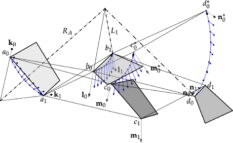
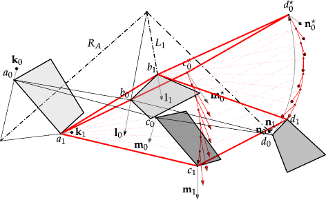
Figure 6. Rotations about $R_{A}$ (top) and about $L_{1}$ (bottom) in the proof of Theorem 11

Proof of Theorem 11.

We consider an elementary quadrilateral $(a_{0},\mathbf{k}_{0})$, …, $(a_{3},\mathbf{k}_{3})$ of the principal contact element net $(a,\mathbf{k})$ and the corresponding quadrilaterals $(b_{0},\mathbf{l}_{0})$, …, $(b_{3},\mathbf{l}_{3})$, and $(c_{0},\mathbf{m}_{0})$, …, $(c_{3},\mathbf{m}_{3})$ under the two Bäcklund transforms. By Lemma 17 there exist uniquely determined contact elements $(d_{0},\mathbf{n}_{0})$, …, $(d_{3},\mathbf{n}_{3})$ that satisfy all distance and angle constraints imposed by the Bäcklund transform. We have to show that these contact elements form the elementary quadrilateral of a principal contact element net. In view of Proposition 18 it is sufficient to show that one neighbouring pair, say $(d_{0},\mathbf{n}_{0})$ and $(d_{1},\mathbf{n}_{1})$, corresponds in two different rotations.

As already argued earlier, there exists a rotation $R$ that maps $(a_{0},\mathbf{k}_{0})$ to $(a_{1},\mathbf{k}_{1})$ and, at the same time, $(b_{0},\mathbf{l}_{0})$ to $(b_{1},\mathbf{l}_{1})$. Its axis $A_{R}$ is spanned by $K_{0}\cap K_{1}$ and $L_{0}\cap L_{1}$ (Figure 6, top).

The rotation $R$ transforms $(c_{0},\mathbf{m}_{0})$ to a contact element $(c^{\star}_{1},\mathbf{m}^{\star}_{1})$ and $(d_{0},\mathbf{n}_{0})$ to a contact element $(d^{\star}_{1},\mathbf{n}^{\star}_{1})$. Since $K_{1}$, $L_{1}$, $N^{\star}_{0}$, $M^{\star}_{0}$ and $K_{1}$, $L_{1}$, $N_{1}$, $M_{1}$ are just two realizations of the axes of the same Bennett linkage (with respective normal feet $a_{1}$, $b_{1}$, $d^{\star}_{0}$, $c^{\star}_{0}$ and $a_{1}$, $b_{1}$, $d_{1}$, $c_{1}$), we can rotate $(d^{\star}_{1},\mathbf{n}^{\star}_{1})$ about $K_{1}$ into $(d_{1},\mathbf{n}_{1})$. (Via Bennett’s linkage, this rotation can be coupled with a rotation of $c^{\star}_{0}$ to $c_{1}$ about the axis $K_{1}$ — but this is not relevant at this point of our proof.) The composition of $R$ with this last rotation (Figure 6, bottom), call it $Q$, is again a rotation $S$ because the axes $R_{A}$ and $L_{1}$ of $R$ and $Q$ intersect. Thus, we have found one rotation that transforms $(d_{0},\mathbf{n}_{0})$ to $(d_{1},\mathbf{n}_{1})$. If we start with the rotation that maps $(a_{0},\mathbf{k}_{0})$ to $(a_{1},\mathbf{k}_{1})$ and $(c_{0},\mathbf{m}_{0})$ to $(c_{1},\mathbf{m}_{1})$ we obtain a second rotation $T$ of $(d_{0},\mathbf{n}_{0})$ to $(d_{1},\mathbf{n}_{1})$. Generically, the two rotations $S$ and $T$ are different, because $L_{0}$ and $M_{0}$ do not intersect. We conclude that the contact elements $(d_{0},\mathbf{n}_{0})$ and $(d_{1},\mathbf{n}_{1})$ satisfy the principal contact element criterion of Proposition 18. ∎

6. Conclusion

In this article we gave a fairly complete geometric treatment of the Bäcklund transform of principal contact element nets. We proved the most relevant results (Theorems 4, 9, and 11) which are typical of this curious surface relation. Moreover, we consider the disclosed relations to discrete kinematics and in particular to discrete rotating motions to be of interest. In this context we would emphasize Theorem 8, which already brings us to open issues. We were unable to provide certain proofs (those of Theorems 8 and 9) and in a way that make the involved calculations manually tractable. There is still room left for simplifications. Moreover, an analytic complement to our geometric reasoning, maybe in the style of [11], would be desirable.

References

- Bennett [1903] G. T. Bennett. A new mechanism. Engineering, 76:777–778, 1903.
- Bennett [1913–1914] G. T. Bennett. The skew isogramm-mechanism. Proc. London Math. Soc., 13(2nd Series):151–173, 1913–1914.
- Bobenko and Suris [2007] A. I. Bobenko and Yu. B. Suris. On organizing principles of discrete differential geometry. Geometry of spheres. Russian Math. Surveys, 62(1):1–43, 2007.
- Bobenko and Suris [2008] A. I. Bobenko and Yu. B. Suris. Discrete Differential Geometrie. Integrable Structure, volume 98 of Graduate texts in mathematics. American Mathematical Society, 2008.
- Bobenko et al. [2010] A. I. Bobenko, H. Pottmann, and J. Wallner. A curvature theory for discrete surfaces based on mesh parallelity. Math. Ann., 348(1), 2010.
- Hunt [1978] K. H. Hunt. Kinematic Geometry of Mechanisms. Oxford Engineering Science Series. Oxford University Press, 1978.
- Husty and Schröcker [2009] M. Husty and H.-P. Schröcker. Algebraic geometry and kinematics. In Ioannis Z. Emiris, Frank Sottile, and Thorsten Theobald, editors, Nonlinear Computational Geometry, volume 151 of The IMA Volumes in Mathematics and its Applications, chapter Algebraic Geometry and Kinematics. Springer, 2009.
- Pottmann and Wallner [2001] H. Pottmann and J. Wallner. Computational Line Geometry. Mathematics and visualization. Springer, Heidelberg, 2001.
- Pottmann and Wallner [2008] H. Pottmann and J. Wallner. The focal geometry of circular and conical meshes. Adv. Comput. Math., 29(3):249–268, 2008.
- Rogers and Schief [2002] C. Rogers and W. K. Schief. Bäcklund and Darboux Transformations. Geometry and Moderns Applications in Soliton Theory. Cambridge Texts in Applied Mathematics. Cambridge University Press, 2002.
- Schief [2003] W. K. Schief. On the unification of classical and novel integrable surfaces. II. Difference geometry. Proc. Roy. Soc. London Ser. A, 459:373–391, 2003.
- Schröcker [2010a] H.-P. Schröcker. Discrete gliding along principal curves. In N. Ando, T. Kanai, J. Mitani, A. Saito, and Y. Yamaguchi, editors, Proceedings of the 14th International Conference on Geometry and Graphics, pages 37–46, Kyoto, 2010a.
- Schröcker [2010b] H.-P. Schröcker. Contributions to four-positions theory with relative rotations. In D. L. Pisla, M. Ceccarelli, M. Husty, and B. J. Corves, editors, New Trends in Mechanism Science. Analysis and Design, volume 5 of Mechanism and Machine Science, pages 21–28. Springer, 2010b.
- Wunderlich [1951] W. Wunderlich. Zur Differenzengeometrie der Flächen konstanter negativer Krümmung. Österreich. Akad. Wiss. Math.-Naturwiss. Kl. S.-B. II, 160(2):39–77, 1951.