CYCU-HEP-10-16
October, 2010

Charmless Hadronic $B$ Decays into a Tensor Meson

Hai-Yang Cheng^1,2 and Kwei-Chou Yang³

¹ Institute of Physics, Academia Sinica

Taipei, Taiwan 115, Republic of China

² C.N. Yang Institute for Theoretical Physics, State University of New York

Stony Brook, New York 11794

³ Department of Physics, Chung Yuan Christian University

Chung-Li, Taiwan 320, Republic of China

Abstract

Two-body charmless hadronic $B$ decays involving a tensor meson in the final state are studied within the framework of QCD factorization (QCDF). Due to the $G$-parity of the tensor meson, both the chiral-even and chiral-odd two-parton light-cone distribution amplitudes of the tensor meson are antisymmetric under the interchange of momentum fractions of the quark and anti-quark in the SU(3) limit. Our main results are: (i) In the naive factorization approach, the decays such as $B^{-}\to\bar{K}_{2}^{*0}\pi^{-}$ and $\overline{B}^{0}\to K_{2}^{*-}\pi^{+}$ with a tensor meson emitted are prohibited owing to the fact that a tensor meson cannot be created from the local $V-A$ or tensor current. Nevertheless, they receive nonfactorizable contributions in QCDF from vertex, penguin and hard spectator corrections. The experimental observation of $B^{-}\to\bar{K}_{2}^{*0}\pi^{-}$ indicates the importance of nonfactorizable effects. (ii) For penguin-dominated $B\to TP$ and $TV$ decays, the predicted rates in naive factorization are usually too small by one to two orders of magnitude. In QCDF, they are enhanced by power corrections from penguin annihilation and nonfactorizable contributions. (iii) The dominant penguin contributions to $B\to K_{2}^{*}\eta^{(^{\prime})}$ arise from the processes: (a) $b\to ss\bar{s}\to s\eta_{s}$ and (b) $b\to sq\bar{q}\to q\bar{K}_{2}^{*}$ with $\eta_{q}=(u\bar{u}+d\bar{d})/\sqrt{2}$ and $\eta_{s}=s\bar{s}$. The interference, constructive for $K_{2}^{*}\eta^{\prime}$ and destructive for $K_{2}^{*}\eta$, explains why $\Gamma(B\to K_{2}^{*}\eta^{\prime})\gg\Gamma(B\to K_{2}^{*}\eta)$. (iv) We use the measured rates of $B\to K_{2}^{*}(\omega,\phi)$ to extract the penguin-annihilation parameters $\rho_{A}^{TV}$ and $\rho_{A}^{VT}$ and the observed longitudinal polarization fractions $f_{L}(K_{2}^{*}\omega)$ and $f_{L}(K_{2}^{*}\phi)$ to fix the phases $\phi_{A}^{VT}$ and $\phi_{A}^{TV}$. (v) The experimental observation that $f_{T}/f_{L}\ll 1$ for $B\to K_{2}^{*}(1430)\phi$, whereas $f_{T}/f_{L}\sim 1$ for $B\to K_{2}^{*}(1430)\omega$ with $f_{T}$ being the transverse polarization fraction, can be accommodated in QCDF, but cannot be dynamically explained at first place. For penguin-dominated $B\to TV$ decays, we find $f_{L}(K_{2}^{*}\rho)\sim f_{L}(K_{2}^{*}\omega)\sim 0.65$ , whereas $f_{L}(K^{*}f_{2})\sim 0.93$. It will be of great interest to measure $f_{L}$ for these modes to test QCDF. Theoretically, transverse polarization is expected to be small in tree-dominated $\overline{B}\to TV$ decays except for the $a_{2}^{-}\rho^{0},~{}a_{2}^{-}\rho^{+},~{}K_{2}^{*0}K^{*-}$ and $K_{2}^{*0}\bar{K}^{*0}$ modes. (vi) For tree-dominated decays, their rates are usually very small except for the $a_{2}^{0}(\pi^{-},\rho^{-}),~{}a_{2}^{+}(\pi^{-},\rho^{-})$ and $f_{2}(\pi^{-},\rho^{-})$ modes with branching fractions of order $10^{-6}$ or even bigger.

I Introduction

In the past few years, BaBar and Belle BaBar:etapK2p ; BaBar:etaK2p ; BaBar:omegaK2p ; BaBar:f2Kp ; BaBar:f2pKp ; BaBar:phiK2p ; BaBar:f2pip ; BaBar:K20pi0 ; BaBar:f2K0 ; BaBar:phiK20 ; Belle:f2Kp ; Belle:f2pKp ; Belle:K20Kp ; Belle:f2K0 have begun to measure several charmless $B$ decay modes involving a light tensor meson $T$ in the final states with the results summarized in Table 1. From the theoretical point of view, the hadronic decays $B\to TM$ with $M=P,V,A$ are of great interest for two reasons: rate deficit and polarization puzzles. First, these decays have been studied in the naive factorization approach Katoch ; Munoz97 ; Munoz:99 ; Kim:2002a ; Kim:2002b ; Kim:2003 ; Munoz ; Verma ; Sharma . The predicted rates are in general too small by one to two orders of magnitude. This implies the importance of $1/m_{b}$ power corrections. Since the nonfactorizable amplitudes such as vertex and penguin corrections, spectator interactions cannot be tackled in naive factorization, it is necessary to go beyond the naive factorization framework. The theoretical frameworks suitable for this purpose include QCD factorization BBNS , perturbative QCD (pQCD) pQCD and soft-collinear effective theory (SCET) SCET

Second, it is known that an unexpectedly large fraction of transverse polarization has been observed in the penguin-dominated $B\to VV$ channels, such as $B\to\phi K^{*},\rho K^{*}$, contrary to the naive expectation of the longitudinal polarization dominance (for a review, see ChengSmith ). However, while the polarization measurement in $B\to\omega K_{2}^{*}(1430)$ indicates a large fraction of transverse polarization $f_{T}$ (see Table 1), the measurement in $B\to\phi K_{2}^{*}(1430)$ is consistent with the longitudinal polarization dominance. Therefore, it is important to understand why $f_{T}/f_{L}\ll 1$ for $B\to\phi K_{2}^{*}(1430)$, whereas $f_{T}/f_{L}\sim 1$ for $B\to\omega K_{2}^{*}(1430)$, even though both are penguin-dominated. The polarization studies for $B\to TV,TA,TT$ will further shed light on the underlying helicity structure of the decay mechanism.

In the present work we shall study charmless $B\to TM$ decays within the framework of QCD factorization. One unique feature of the tensor meson is that it cannot be created from the $V-A$ or tensor current. Hence, the decay with a tensor meson emitted, for example, $B^{-}\to\bar{K}_{2}^{*0}\pi^{-}$, is prohibited in naive factorization. The experimental observation of this penguin-dominated mode with a sizable rate implies the importance of nonfactorizable effects which will be addressed in QCDF.

The layout of this work is as follows. We study the physical properties of tensor mesons such as decay constants, form factors, light-cone distribution amplitudes and helicity projection operators in Sec. 2 and specify various input parameters. Then we work out in details the next-to-leading order (NLO) corrections to $B\to TP,TV$ decays in Sec. 3 and present numerical results and discussions in Sec. 4. Conclusions are given in Sec. 5. Appendix A is devoted to a recapitulation of the ISGW model. Decay amplitudes and explicit expressions of helicity-dependent annihilation amplitudes are shown in Appendices B and C, respectively. A mini review of of the $\eta-\eta^{\prime}$ mixing is given in Appendix D.

Table 1: Experimental branching fractions (in units of $10^{-6}$) and the longitudinal polarization fractions $f_{L}$ for $B$ decays to final states containing a tensor meson. Data are taken from BaBar:etapK2p ; BaBar:etaK2p ; BaBar:omegaK2p ; BaBar:f2Kp ; BaBar:f2pKp ; BaBar:phiK2p ; BaBar:f2pip ; BaBar:K20pi0 ; BaBar:f2K0 ; BaBar:phiK20 ; Belle:f2Kp ; Belle:f2pKp ; Belle:K20Kp ; Belle:f2K0 .

Mode	${\cal B}$	$f_{L}$	Mode	${\cal B}$	$f_{L}$
${\cal B}(B^{+}\to K_{2}^{*}(1430)^{+}\omega)$	$21.5\pm 4.3$	$0.56\pm 0.11$	${\cal B}(B^{0}\to K_{2}^{*}(1430)^{0}\omega)$	$10.1\pm 2.3$	$0.45\pm 0.12$
${\cal B}(B^{+}\to K_{2}^{*}(1430)^{+}\phi)$	$8.4\pm 2.1$	$0.80\pm 0.10$	${\cal B}(B^{0}\to K_{2}^{*}(1430)^{0}\phi)$	$7.5\pm 1.0$	$0.901^{+0.059}_{-0.069}$
${\cal B}(B^{+}\to K_{2}^{*}(1430)^{+}\eta)$	$9.1\pm 3.0$		${\cal B}(B^{0}\to K_{2}^{*}(1430)^{0}\eta)$	$9.6\pm 2.1$
${\cal B}(B^{+}\to K_{2}^{*}(1430)^{+}\eta^{\prime})$	$28.0^{+5.3}_{-5.0}$		${\cal B}(B^{0}\to K_{2}^{*}(1430)^{0}\eta^{\prime})$	$13.7^{+3.2}_{-3.1}$
${\cal B}(B^{+}\to K_{2}^{*}(1430)^{0}\pi^{+})$	$5.6^{+2.2}_{-1.4}$		${\cal B}(B^{0}\to K_{2}^{*}(1430)^{+}\pi^{-})$	$<6.3$
${\cal B}(B^{+}\to K_{2}^{*}(1430)^{0}K^{+})$	$<1.1$		${\cal B}(B^{0}\to K_{2}^{*}(1430)^{0}\pi^{0})$	$<4.0$
${\cal B}(B^{+}\to f_{2}(1270)K^{+})$	$1.06^{+0.28}_{-0.29}$		${\cal B}(B^{0}\to f_{2}(1270)K^{0})$	$2.7^{+1.3}_{-1.2}$
${\cal B}(B^{+}\to f_{2}(1270)\pi^{+})$	$1.57^{+0.69}_{-0.49}$
${\cal B}(B^{+}\to f^{\prime}_{2}(1525)K^{+})$	$<7.7$
${\cal B}(B^{+}\to a_{2}(1320)^{0}K^{+})$	$<45$

II Physical properties of tensor mesons

II.1 Tensor mesons

The observed $J^{P}=2^{+}$ tensor mesons $f_{2}(1270)$, $f_{2}^{\prime}(1525)$, $a_{2}(1320)$ and $K_{2}^{*}(1430)$ form an SU(3) $1\,^{3}P_{2}$ nonet. The $q\bar{q}$ content for isodoublet and isovector tensor resonances is obvious. Just as the $\eta$-$\eta^{\prime}$ mixing in the pseudoscalar case, the isoscalar tensor states $f_{2}(1270)$ and $f^{\prime}_{2}(1525)$ also have a mixing, and their wave functions are defined by

$$f_{2}(1270) = {1\over\sqrt{2}}(f_{2}^{u}+f_{2}^{d})\cos\theta_{f_{2}}+f_{2}^{s}\sin\theta_{f_{2}}~{},$$

$$f^{\prime}_{2}(1525) = {1\over\sqrt{2}}(f_{2}^{u}+f_{2}^{d})\sin\theta_{f_{2}}-f_{2}^{s}\cos\theta_{f_{2}}~{},$$ (1)

with $f_{2}^{u}\equiv u\bar{u}$ and likewise for $f_{2}^{d,s}$. Since $\pi\pi$ is the dominant decay mode of $f_{2}(1270)$ whereas $f_{2}^{\prime}(1525)$ decays predominantly into $K\overline{K}$ (see Ref. PDG ), it is obvious that this mixing angle should be small. More precisely, it is found that $\theta_{f_{2}}=7.8^{\circ}$ Li and $(9\pm 1)^{\circ}$ PDG . Therefore, $f_{2}(1270)$ is primarily an $(u\bar{u}+d\bar{d})/\sqrt{2}$ state, while $f^{\prime}_{2}(1525)$ is dominantly $s\bar{s}$.

For a tensor meson, the polarization tensors $\epsilon_{(\lambda)}^{\mu\nu}$ with helicity $\lambda$ can be constructed in terms of the polarization vectors of a massive vector state moving along the $z$-axis Berger:2000wt

$$\epsilon(0)^{*\mu}=(P_{3},0,0,E)/m_{T},\quad\epsilon(\pm 1)^{*\mu}=(0,\mp 1,+i,0)/\sqrt{2},$$ (2)

and are given by

$$\epsilon^{\mu\nu}_{(\pm 2)} \equiv \epsilon(\pm 1)^{\mu}\epsilon(\pm 1)^{\nu},$$ (3)

$$\epsilon^{\mu\nu}_{(\pm 1)} \equiv \sqrt{\frac{1}{2}}[\epsilon(\pm 1)^{\mu}\epsilon(0)^{\nu}+\epsilon(0)^{\mu}\epsilon(\pm 1)^{\nu}],$$ (4)

$$\epsilon^{\mu\nu}_{(0)} \equiv \sqrt{\frac{1}{6}}[\epsilon(+1)^{\mu}\epsilon(-1)^{\nu}+\epsilon(-1)^{\mu}\epsilon(+1)^{\nu}]+\sqrt{\frac{2}{3}}\epsilon(0)^{\mu}\epsilon(0)^{\nu}.$$ (5)

The polarization $\epsilon_{\mu\nu}^{(\lambda)}$ can be decomposed in the frame formed by the two light-like vectors, $z_{\mu}$ and $p_{\nu}\equiv P_{\nu}-z_{\nu}m_{T}^{2}/(2pz)$ with $P_{\nu}$ and $m_{T}$ being the momentum and mass of the tensor meson, respectively, and their orthogonal plane Ball:1998sk ; Ball:1998ff . The transverse component that we use thus reads

$$\epsilon^{(\lambda)}_{\perp\,\mu\nu}z^{\nu}=\epsilon^{(\lambda)}_{\mu\nu}z^{\nu}-\epsilon^{(\lambda)}_{\parallel\mu\nu}z^{\nu}=\epsilon^{(\lambda)}_{\mu\nu}z^{\nu}-\frac{\epsilon^{(\lambda)}_{\alpha\nu}z^{\alpha}z^{\nu}}{pz}\left(p_{\mu}-\frac{m_{T}^{2}}{2pz}\,z_{\mu}\right)\,.$$ (6)

The polarization tensor $\epsilon^{(\lambda)}_{\alpha\beta}$ satisfies the relations

$$\epsilon_{\mu\nu}^{(\lambda)}=\epsilon_{\nu\mu}^{(\lambda)},\qquad\epsilon^{\mu}_{(\lambda)\mu}=0,\qquad P_{\mu}\epsilon_{(\lambda)}^{\mu\nu}=P_{\nu}\epsilon_{(\lambda)}^{\mu\nu}=0,\quad\epsilon^{(\lambda)}_{\mu\nu}\big{(}\epsilon^{(\lambda^{\prime})\mu\nu}\big{)}^{*}=\delta_{\lambda\lambda^{\prime}}.$$ (7)

The completeness relation reads

$$\sum_{\lambda}\epsilon^{(\lambda)}_{\mu\nu}\left(\epsilon^{(\lambda)}_{\rho\sigma}\right)^{\ast}=\frac{1}{2}M_{\mu\rho}M_{\nu\sigma}+\frac{1}{2}M_{\mu\sigma}M_{\nu\rho}-\frac{1}{3}M_{\mu\nu}M_{\rho\sigma}\,,$$ (8)

where $M_{\mu\nu}=g_{\mu\nu}-P_{\mu}P_{\nu}/m_{T}^{2}$.

II.2 Decay constants

Decay constants of the vector meson are defined as

$$\langle V(P,\epsilon)|\bar{q}_{2}\gamma_{\mu}q_{1}|0\rangle = -if_{V}m_{V}\epsilon^{*}_{\mu},$$

$$\langle V(P,\epsilon)|\bar{q}_{2}\sigma_{\mu\nu}q_{1}|0\rangle = -f_{V}^{\perp}(\epsilon_{\mu}^{*}P_{\nu}-\epsilon_{\nu}^{*}P_{\mu})\,.$$ (9)

Contrary to the vector meson case, a ${}^{3}P_{2}$ tensor meson with $J^{PC}=2^{++}$ cannot be produced through the local $V-A$ and tensor currents. To see this, we notice that

$$\langle T(P,\lambda)|V_{\mu}|0\rangle = a\epsilon^{*(\lambda)}_{\mu\nu}P^{\nu}+b\epsilon^{*(\lambda)\nu}_{~{}\nu}P_{\mu}=0,$$ (10)

$$\langle T(P,\lambda)|A_{\mu}|0\rangle = \varepsilon_{\mu\nu\rho\sigma}P^{\nu}\epsilon_{(\lambda)}^{\rho\sigma*}=0,$$ (11)

where use of Eq. (7) has been made. Nevertheless, a tensor meson can be created from these local currents involving covariant derivatives:

$$\langle T(P,\lambda)|J_{\mu\nu}(0)|0\rangle = f_{T}m_{T}^{2}\epsilon^{*(\lambda)}_{\mu\nu},$$

$$\langle T(P,\lambda)|J^{\perp}_{\mu\nu\alpha}(0)|0\rangle = -if_{T}^{\perp}m_{T}(\epsilon_{\mu\alpha}^{(\lambda)*}P_{\nu}-\epsilon_{\nu\alpha}^{(\lambda)*}P_{\mu}),$$ (12)

where

$$J_{\mu\nu}(0) = \frac{1}{2}\left(\bar{q}_{1}(0)\gamma_{\mu}i\stackrel{{\scriptstyle\leftrightarrow}}{{D}}_{\nu}q_{2}(0)+\bar{q}_{1}(0)\gamma_{\nu}i\stackrel{{\scriptstyle\leftrightarrow}}{{D}}_{\mu}q_{2}(0)\right),$$

$$J^{\perp}_{\mu\nu\alpha}(0) = \bar{q}_{1}(0)\sigma_{\mu\nu}i\stackrel{{\scriptstyle\leftrightarrow}}{{D}}_{\alpha}q_{2}(0),$$ (13)

and $\stackrel{{\scriptstyle\leftrightarrow}}{{D}}_{\mu}=\stackrel{{\scriptstyle\rightarrow}}{{D}}_{\mu}-\stackrel{{\scriptstyle\leftarrow}}{{D}}_{\mu}$ with $\stackrel{{\scriptstyle\rightarrow}}{{D}}_{\mu}=\stackrel{{\scriptstyle\rightarrow}}{{\partial}}_{\mu}+ig_{s}A^{a}_{\mu}\lambda^{a}/2$ and $\stackrel{{\scriptstyle\leftarrow}}{{D}}_{\mu}=\stackrel{{\scriptstyle\leftarrow}}{{\partial}}_{\mu}-ig_{s}A^{a}_{\mu}\lambda^{a}/2$.

The decay constant $f_{T}$ of the tensor meson has been estimated using QCD sum rules for the tensor mesons $f_{2}(1270)$ Aliev:1981ju and $K^{*}_{2}(1430)$ Aliev:2009nn and the tensor-meson-dominance hypothesis for $f_{2}(1270)$ Aliev:1981ju ; Terazawa:1990es ; Suzuki:1993zs . The previous sum rule predictions are Aliev:1981ju ; Aliev:2009nn

$$f_{f_{2}(1270)}(\mu=1~{}{\rm GeV}) \simeq 0.08\,m_{f_{2}(1270)}=102~{}{\rm MeV}\,,$$

$$f_{K^{*}_{2}(1430)}(\mu=1~{}{\rm GeV}) \simeq (0.10\pm 0.01)\,m_{K^{*}_{2}(1430)}=(143\pm 14)\,{\rm MeV}\,.$$ (14)

Recently, we have derived a sum rule for $f_{T}(\mu)f_{T}^{\bot}(\mu)$ and revisited the sum-rule analysis for $f_{T}(\mu)$. Our results of $f_{T}$ and $f_{T}^{\bot}$ for various tensor mesons are shown in Table 4 below CKY . Our sum rule results are in good agreement with Aliev:1981ju for $f_{f_{2}(1270)}$, but smaller than that of Aliev:2009nn for $f_{K_{2}^{*}(1430)}$. The decay constants for $f_{2}(1270)$ and $f_{2}^{\prime}(1525)$ also can be extracted based on the hypothesis of tensor meson dominance together with the data of $\Gamma(f_{2}\to\pi\pi)$ and $\Gamma(f^{\prime}_{2}\to K\bar{K})$. We found that CKY

$$f_{f_{2}(1270)}\simeq(0.085\pm 0.001)m_{f_{2}(1270)}=(108\pm 1)\,{\rm MeV}\,,$$

$$f_{f^{\prime}_{2}(1525)}\simeq(0.089\pm 0.003)m_{f^{\prime}_{2}(1525)}=(136\pm 5)\,{\rm MeV}\,.$$ (15)

They are in accordance with the sum rule predictions shown in Table 4.

II.3 Form factors

Form factors for $B\to P,V,T$ transitions are defined by BSW ; Hatanaka:2009gb ; Wei

$$\langle P(P)|V_{\mu}|B(p_{B})\rangle = \left(P_{\mu}+(p_{B})_{\mu}-{m_{B}^{2}-m_{P}^{2}\over q^{2}}\,q_{\mu}\right)F_{1}^{BP}(q^{2})+{m_{B}^{2}-m_{P}^{2}\over q^{2}}q_{\mu}\,F_{0}^{BP}(q^{2}),$$

$$\langle{V}(P,\lambda)|V_{\mu}|{B}(p_{B})\rangle = -i\frac{2}{m_{B}+m_{V}}\varepsilon_{\mu\nu\alpha\beta}\epsilon_{(\lambda)}^{*\nu}p_{B}^{\alpha}P^{\beta}V^{BV}(q^{2}),$$

$$\langle V(P,\lambda)|A_{\mu}|{B}(p_{B})\rangle = 2m_{V}\frac{\epsilon^{(\lambda)*}\cdot p_{B}}{q^{2}}q_{\mu}A_{0}^{BV}(q^{2})+(m_{B}+m_{V})\left[\epsilon^{(\lambda)*}_{\mu}-\frac{e^{(\lambda)*}\cdot p_{B}}{q^{2}}q_{\mu}\right]A_{1}^{BV}(q^{2})$$

$$-{\epsilon^{(\lambda)*}\cdot p_{B}\over m_{B}+m_{V}}\left[P_{\mu}+(p_{B})_{\mu}-{m_{B}^{2}-m_{V}^{2}\over q^{2}}q_{\mu}\right]A_{2}^{BV}(q^{2})$$

$$\langle{T}(P,\lambda)|V_{\mu}|{B}(p_{B})\rangle = -i\frac{2}{m_{B}+m_{T}}\varepsilon_{\mu\nu\alpha\beta}e_{(\lambda)}^{*\nu}p_{B}^{\alpha}P^{\beta}V^{BT}(q^{2}),$$

$$\langle T(P,\lambda)|A_{\mu}|{B}(p_{B})\rangle = 2m_{T}\frac{e^{(\lambda)*}\cdot p_{B}}{q^{2}}q_{\mu}A_{0}^{BT}(q^{2})+(m_{B}+m_{T})\left[e^{(\lambda)*}_{\mu}-\frac{e^{(\lambda)*}\cdot p_{B}}{q^{2}}q_{\mu}\right]A_{1}^{BT}(q^{2})$$ (16)

$$-{e^{(\lambda)*}\cdot p_{B}\over m_{B}+m_{T}}\left[P_{\mu}+(p_{B})_{\mu}-{m_{B}^{2}-m_{T}^{2}\over q^{2}}q_{\mu}\right]A_{2}^{BT}(q^{2}),$$

where $q_{\mu}=(p_{B}-P)_{\mu}$ and $e^{*\mu}_{(\lambda)}\equiv\epsilon^{*\mu\nu}_{(\lambda)}p_{{}_{B\nu}}/m_{B}$. Throughout the paper we have adopted the convention $\varepsilon^{0123}=-1$.

In the Isgur-Scora-Grinstein-Wise (ISGW) model ISGW , the general expression for the $B\to T$ transition is parametrized as

$$\langle T(P,\lambda)|(V-A)_{\mu}|B(p_{B})\rangle = ih(q^{2})\varepsilon_{\mu\nu\rho\sigma}\epsilon^{*\nu\alpha}p_{B\alpha}(p_{B}+P)^{\rho}q^{\sigma}-k(q^{2})\epsilon^{*}_{\mu\nu}p_{B}^{\nu}$$ (17)

$$- b_{+}(q^{2})\epsilon^{*}_{\alpha\beta}p_{B}^{\alpha}p_{B}^{\beta}(p_{B}+P)_{\mu}-b_{-}(q^{2})\epsilon^{*}_{\alpha\beta}p_{B}^{\alpha}p_{B}^{\beta}q_{\mu},$$

where the form factor $k$ is dimensionless, and the canonical dimension of $h,b_{+}$ and $b_{-}$ is $-2$. The relations between these two different sets of form factors are

$$V^{BT}(q^{2})=m_{B}(m_{B}+m_{T})h(q^{2}),\qquad A_{1}^{BT}(q^{2})={m_{B}\over m_{B}+m_{T}}k(q^{2}),$$ (18)

$$A_{2}^{BT}(q^{2})=-m_{B}(m_{B}+m_{T})b_{+}(q^{2}),\quad A_{0}^{BT}(q^{2})={m_{B}\over 2m_{T}}[k^{2}(q^{2})+(m_{B}^{2}-m_{T}^{2})b_{+}(q^{2})+q^{2}b_{-}(q^{2})].$$

The $B\to T$ transition form factors have been evaluated in the ISGW model ISGW and its improved version, ISGW2 ISGW2 , the covariant light-front quark model (CLFQ) CCH , the light-cone sum rule (LCSR) approach kcy , the large energy effective theory (LEET) Charles ; Ebert ; Datta and the pQCD approach Wei . In LEET, form factors are evaluated at large recoil and all the form factors in the LEET limit to be specified below can be parametrized in terms of two independent universal form factors $\zeta_{\bot}$ and $\zeta_{\parallel}$ Hatanaka:2009gb :

$$V^{BT}(q^{2}) = {m_{{}_{T}}\over|\vec{p}_{{}_{T}}|}\left(1+{m_{T}\over m_{B}}\right)\zeta_{\bot}(q^{2}),$$

$$A_{0}^{BT}(q^{2}) = {m_{{}_{T}}\over|\vec{p}_{{}_{T}}|}\left[\left(1-{m_{T}^{2}\over m_{B}E_{T}}\right)\zeta_{\parallel}(q^{2})+{m_{T}\over m_{B}}\zeta_{\bot}(q^{2})\right],$$

$$A_{1}^{BT}(q^{2}) = {m_{{}_{T}}\over|\vec{p}_{{}_{T}}|}\left({2E_{T}\over m_{B}+m_{T}}\right)\zeta_{\bot}(q^{2}),$$

$$A_{2}^{BT}(q^{2}) = {m_{{}_{T}}\over|\vec{p}_{{}_{T}}|}\left(1+{m_{T}\over m_{B}}\right)\left[\zeta_{\bot}(q^{2})-{m_{T}\over E_{T}}\zeta_{\parallel}(q^{2})\right],$$ (19)

where $E_{T}$ is the energy of the tensor meson

$$E_{T}={m_{B}\over 2}\left(1+{m_{T}^{2}-q^{2}\over m_{B}^{2}}\right).$$ (20)

In the LEET limit,

$$E_{T},m_{B}\gg m_{T},\Lambda_{\rm QCD}.$$ (21)

Using the recent analysis of tensor meson distribution amplitudes CKY , one of us (KCY) has calculated the form factors of $B$ decays into tensor mesons using the LCSR approach kcy . The LCSR results are close to LEET and pQCD calculations.

The $B\to a_{2}(1320),f_{2q}=(u\bar{u}+d\bar{d})/\sqrt{2},K_{2}^{*}(1430)$ transition form factors calculated in various models at the maximal recoil $q^{2}=0$ are summarized in Table 2. The ISGW model ISGW is based on the non-relativistic constituent quark picture. In general, the form factors evaluated in the ISGW model are reliable only at $q^{2}=q^{2}_{m}\equiv(m_{B}-m_{T})^{2}$, the maximum momentum transfer. The reason is that the form-factor $q^{2}$ dependence in the ISGW model is proportional to exp[$-(q^{2}_{m}-q^{2})$] and hence the form factor decreases exponentially as a function of $(q^{2}_{m}-q^{2})$ (see Appendix A for details). This has been improved in the ISGW2 model ISGW2 in which the form factor has a more realistic behavior at large $(q^{2}_{m}-q^{2})$ which is expressed in terms of a certain polynomial term. As noticed in Kim:2003 , form factors are increased in the ISGW2 model so that the branching fractions of $B\to TM$ decays are enhanced by about an order of magnitude compared to the estimates based on the ISGW model.

Table 2: $B\to T$ transition form factors at $q^{2}=0$ evaluated in the ISGW2, CLFQ, LCSR, LEET and pQCD models. The CLFQ results are obtained by first calculating the form factors $h(q^{2}),b_{+}(q^{2})$ and $b_{-}(q^{2})$ using the covariant light-front approach and $k(q^{2})$ from the heavy quark symmetry relation Eq. (22) and then converted them into the form-factor set $V(q^{2})$ and $A_{0,1,2}(q^{2})$. To compute the form factors in LEET we have applied $\zeta_{\bot}(0)=0.28\pm 0.04$ and $\zeta_{\parallel}(0)=0.22\pm 0.03$ . LCSR and pQCD results are taken from kcy and Wei , respectively.

$F$	ISGW2	CLFQ	LCSR	LEET	pQCD	$F$	ISGW2	CLFQ	LCSR	LEET	pQCD
$V^{Ba_{2}}$	0.32	0.28	$0.18\pm 0.02$	$0.18\pm 0.03$	$0.18^{+0.05}_{-0.04}$	$A_{0}^{Ba_{2}}$	$0.20$	$0.24$	$0.21\pm 0.04$	$0.14\pm 0.02$	$0.18^{+0.06}_{-0.04}$
$A_{1}^{Ba_{2}}$	$0.16$	$0.21$	$0.14\pm 0.02$	$0.13\pm 0.02$	$0.11^{+0.03}_{-0.03}$	$A_{2}^{Ba_{2}}$	0.14	0.19	$0.09\pm 0.02$	$0.13\pm 0.02$	$0.06^{+0.02}_{-0.01}$
$V^{Bf_{2q}}$	0.32	0.28	$0.18\pm 0.02$	$0.18\pm 0.02$	$0.12^{+0.03}_{-0.03}$	$A_{0}^{Bf_{2q}}$	$0.20$	$0.25$	$0.20\pm 0.04$	$0.13\pm 0.02$	$0.13^{+0.04}_{-0.03}$
$A_{1}^{Bf_{2q}}$	$0.16$	$0.21$	$0.14\pm 0.02$	$0.12\pm 0.02$	$0.08^{+0.02}_{-0.02}$	$A_{2}^{Bf_{2q}}$	0.14	0.19	$0.10\pm 0.02$	$0.13\pm 0.02$	$0.04^{+0.01}_{-0.01}$
$V^{BK_{2}^{*}}$	0.38	0.29	$0.16\pm 0.02$	$0.21\pm 0.03$	$0.21^{+0.06}_{-0.05}$	$A_{0}^{BK_{2}^{*}}$	0.27	$0.23$	$0.25\pm 0.04$	$0.15\pm 0.02$	$0.18^{+0.05}_{-0.04}$
$A_{1}^{BK_{2}^{*}}$	$0.24$	$0.22$	$0.14\pm 0.02$	$0.14\pm 0.02$	$0.13^{+0.04}_{-0.03}$	$A_{2}^{BK_{2}^{*}}$	0.22	0.21	$0.05\pm 0.02$	$0.14\pm 0.02$	$0.08^{+0.03}_{-0.02}$

The CLFQ model is a relativistic quark model in which a consistent and fully relativistic treatment of quark spins and the center-of-mass motion is carried out. This model is very suitable to study hadronic form factors. Especially, as the recoil momentum increases (corresponding to a decreasing $q^{2}$), we need to start considering relativistic effects seriously. In particular, at the maximum recoil point $q^{2}=0$ where the final-state meson could be highly relativistic, it is expected that the corrections to non-relativistic quark model will be sizable in this case.

The CLFQ and ISGW2 model predictions for $B\to T$ transition form factors differ mainly in two aspects: (i) when $q^{2}$ increases, $h(q^{2})$, $b_{+}(q^{2})$ and $b_{-}(q^{2})$ increases more rapidly in the former and (ii) the form factor $k$ obtained in both models is quite different, for example, $k^{BK_{2}^{*}}(0)=0.015$ in the former and 0.293 in the latter. Indeed, it has been noticed CCH that among the four $B\to T$ transition form factors, the one $k(q^{2})$ is particularly sensitive to $\beta_{T}$, a parameter describing the tensor-meson wave function, and that $k(q^{2})$ at zero recoil shows a large deviation from the heavy quark symmetry relation. It is not clear to us if the very complicated analytic expression for $k(q^{2})$ in Eq. (3.29) of CCH is complete. To overcome this difficulty, it was pointed out in CCH that one may apply the heavy quark symmetry relation to obtain $k(q^{2})$ for $B\to T$ transition

$$k(q^{2})=\,m_{B}m_{T}\left(1+{m_{B}^{2}+m_{T}^{2}-q^{2}\over 2m_{B}m_{T}}\right)\left[h(q^{2})-{1\over 2}b_{+}(q^{2})+{1\over 2}b_{-}(q^{2})\right].$$ (22)

In Table 2 the CLFQ results are obtained by first calculating the form factors $h(q^{2}),b_{+}(q^{2})$ and $b_{-}(q^{2})$ using the covariant light-front approach CCH and $k(q^{2})$ from the heavy quark symmetry relation Eq. (22) and then converted them into the form-factor set $V(q^{2})$ and $A_{0,1,2}(q^{2})$.

Table 3: $B\to T$ transition form factors obtained in the covariant light-front model and fitted to the 3-parameter form Eq. (23).

$F$	$F(0)$	$a$	$b$	$F$	$F(0)$	$a$	$b$
$V^{Ba_{2}}$	0.28	2.19	$2.22$	$A_{0}^{Ba_{2}}$	$0.24$	$1.28$	$0.84$
$A_{1}^{Ba_{2}}$	$0.21$	$1.38$	$0.47$	$A_{2}^{Ba_{2}}$	0.19	$1.93$	$1.69$
$V^{Bf_{2q}}$	0.28	2.19	$2.22$	$A_{0}^{Bf_{2q}}$	$0.25$	$1.37$	$0.95$
$A_{1}^{Bf_{2q}}$	$0.21$	$1.39$	$0.46$	$A_{2}^{Bf_{2q}}$	0.19	$1.93$	$1.69$
$V^{BK_{2}^{*}}$	0.29	2.17	$2.22$	$A_{0}^{BK_{2}^{*}}$	$0.23$	$1.23$	$0.74$
$A_{1}^{BK_{2}^{*}}$	$0.22$	1.42	$0.50$	$A_{2}^{BK_{2}^{*}}$	0.21	1.96	$1.79$

Form factors in the CLFQ model are first calculated in the spacelike region and their momentum dependence is fitted to a 3-parameter form

$$F(q^{2})=\,{F(0)\over 1-a(q^{2}/m_{B}^{2})+b(q^{2}/m_{B}^{2})^{2}}\,.$$ (23)

The parameters $a$, $b$ and $F(0)$ are first determined in the spacelike region. This parametrization is then analytically continued to the timelike region to determine the physical form factors at $q^{2}\geq 0$. The results are exhibited in Table 3. The momentum dependence of the form factors in the LCSR approach can be found in kcy , while a slightly different parametrization

$$F(q^{2})=\,{F(0)\over(1-q^{2}/m_{B}^{2})[1-a\,q^{2}/m_{B}^{2}+b\,q^{4}/m_{B}^{4}]}$$ (24)

is used in the pQCD approach for the calculations of the form-factor $q^{2}$ dependence Wei .

For the calculation in LEET, we have followed Hatanaka:2009sj to use $\zeta_{\bot}(0)=0.28\pm 0.04$ and $\zeta_{\parallel}(0)=0.22\pm 0.03$. For the $q^{2}$ dependence, we shall use

$$\zeta_{\bot,\parallel}^{T}(q^{2})={\zeta_{\bot,\parallel}^{T}(0)\over(1-q^{2}/m_{B}^{2})^{2}}.$$ (25)

For the ISGW2 model, the $q^{2}$ dependence of the form factors is governed by Eq. (125).

II.4 Light-cone distribution amplitudes

The light-cone distribution amplitudes (LCDAs) of the tensor meson are defined as CKY

$$\langle T(P,\lambda)|\bar{q}_{1}(y)\gamma_{\mu}{q_{2}}(x)|0\rangle = -if_{T}m^{2}_{T}\int\limits_{0}^{1}\!du\,e^{i(uPy+\bar{u}Px)}\Bigg{\{}P_{\mu}\frac{\epsilon^{(\lambda)*}_{\alpha\beta}z^{\alpha}z^{\beta}}{(Pz)^{2}}\,\Phi^{T}_{\parallel}(u)+\Bigg{(}\frac{\epsilon^{(\lambda)*}_{\mu\alpha}z^{\alpha}}{Pz}$$ (26)

$$- P_{\mu}\frac{\epsilon^{(\lambda)*}_{\beta\alpha}z^{\beta}z^{\alpha}}{(Pz)^{2}}\Bigg{)}\,g_{v}(u)-\frac{1}{2}z_{\mu}\frac{\epsilon^{(\lambda)*}_{\alpha\beta}z^{\alpha}z^{\beta}}{(Pz)^{3}}m_{T}^{2}\,\bar{g}_{3}(u)+{\cal O}(z^{2})\Bigg{\}}\,,$$

$$\langle T(P,\lambda)|\bar{q}_{1}(y)\gamma_{\mu}\gamma_{5}q_{2}(x)|0\rangle = -if_{T}m_{T}^{2}\int\limits_{0}^{1}\!du\,e^{i(uPy+\bar{u}Px)}\varepsilon_{\mu\nu\alpha\beta}{z^{\nu}P^{\alpha}}\epsilon_{(\lambda)}^{*\beta\delta}z_{\delta}\,{1\over 2Pz}\,g_{a}(u)\,,$$ (27)

$$\langle T(P,\lambda)|\bar{q}_{1}(y)\sigma_{\mu\nu}q_{2}(x)|0\rangle = -f_{T}^{\perp}m_{T}\int\limits_{0}^{1}\!du\,e^{i(uPy+\bar{u}Px)}\Bigg{\{}\left[\epsilon^{(\lambda)*}_{\mu\alpha}z^{\alpha}P_{\nu}-\epsilon^{(\lambda)*}_{\nu\alpha}z^{\alpha}P_{\mu}\right]\frac{1}{Pz}\Phi^{T}_{\perp}(u)$$ (28)

$$+ (P_{\mu}z_{\nu}-P_{\nu}z_{\mu})\frac{m_{T}^{2}\epsilon^{(\lambda)*}_{\alpha\beta}z^{\alpha}z^{\beta}}{(Pz)^{3}}\bar{h}_{t}(u)$$

$$+ \frac{1}{2}\left[\epsilon^{(\lambda)*}_{\mu\alpha}z^{\alpha}z_{\nu}-\epsilon^{(\lambda)*}_{\nu\alpha}z^{\alpha}z_{\mu}\right]\frac{m_{T}^{2}}{(Pz)^{2}}\bar{h}_{3}(u)+{\cal O}(z^{2})\Bigg{\}}\,,$$

$$\langle T(P,\lambda)|\bar{q}_{1}(y)q_{2}(x)|0\rangle = -f_{T}^{\perp}m_{T}^{3}\int\limits_{0}^{1}\!du\,e^{i(uPy+\bar{u}Px)}\frac{\epsilon^{(\lambda)*}_{\alpha\beta}z^{\alpha}z^{\beta}}{2Pz}h_{s}(u)\,,$$ (29)

where $\bar{g}_{3}=g_{3}+\Phi^{T}_{\parallel}-2g_{v}$, $\bar{h}_{t}=h_{t}-{1\over 2}(\Phi^{T}_{\bot}+h_{3})$, $\bar{h}_{3}=h_{3}-\Phi_{\bot}^{T}$, and $z\equiv y-x$. Here $\Phi^{T}_{\parallel},\Phi^{T}_{\perp}$ are twist-2 LCDAs, $g_{v},g_{a},h_{t},h_{s}$ twist-3 ones, and $g_{3},h_{3}$ twist-4. In the SU(3) limit, due to the $G$-parity of the tensor meson, $\Phi^{T}_{\parallel},\Phi^{T}_{\perp},g_{v},g_{a},h_{t},h_{s},g_{3}$ and $h_{3}$ are antisymmetric under the replacement $u\to 1-u$ CKY .

Using the QCD equations of motion Ball:1998sk ; Ball:1998ff , the two-parton distribution amplitudes $g_{v},g_{a},h_{t}$ and $h_{s}$ can be represented in terms of $\Phi^{T}_{\parallel,\perp}$ and three-parton distribution amplitudes. Neglecting the three-parton distribution amplitudes containing gluons and terms proportional to light quark masses, twist-3 LCDAs $g_{a},g_{v},h_{t}$ and $h_{s}$ are related to twist-2 ones through the Wandzura-Wilczek (WW) relations:

$$g_{v}^{WW}(u) = \int\limits_{0}^{u}dv\,\frac{\Phi^{T}_{\parallel}(v)}{\bar{v}}+\int\limits_{u}^{1}dv\,\frac{\Phi^{T}_{\parallel}(v)}{v}\,,$$

$$g_{a}^{WW}(u) = 2\bar{u}\int\limits_{0}^{u}dv\,\frac{\Phi^{T}_{\parallel}(v)}{\bar{v}}+2u\int\limits_{u}^{1}dv\,\frac{\Phi^{T}_{\parallel}(v)}{v}\,,$$

$$h_{t}^{WW}(u) = \frac{3}{2}(2u-1)\left(\int\limits_{0}^{u}dv\,\frac{\Phi^{T}_{\perp}(v)}{\bar{v}}-\int\limits_{u}^{1}dv\,\frac{\Phi^{T}_{\perp}(v)}{v}\right)\,,$$

$$h_{s}^{WW}(u) = 3\left(\bar{u}\int\limits_{0}^{u}dv\,\frac{\Phi^{T}_{\perp}(v)}{\bar{v}}+u\int\limits_{u}^{1}dv\,\frac{\Phi^{T}_{\perp}(v)}{v}\right)\,.$$ (30)

These WW relations further give us

$${1\over 4}{g^{\prime}_{a}(u)}+{1\over 2}g_{v}(u)=\int_{u}^{1}\frac{\Phi^{T}_{\parallel}(v)}{v}dv\equiv\Phi^{T}_{+}(u)\,,$$

$${1\over 4}{g^{\prime}_{a}(u)}-{1\over 2}g_{v}(u)=-\int_{0}^{u}\frac{\Phi^{T}_{\parallel}(v)}{\bar{v}}dv\equiv-\Phi^{T}_{-}(u)\,,$$

$$h^{\prime}_{s}(u)=-3\Bigg{[}\int_{0}^{u}\frac{\Phi^{T}_{\perp}(v)}{\bar{v}}dv-\int_{u}^{1}\frac{\Phi^{T}_{\perp}(v)}{v}dv\Bigg{]}\equiv-3\Phi_{t}(u),$$ (31)

$$\int_{0}^{u}dv\big{(}\Phi^{T}_{\perp}(v)-{2\over 3}h_{t}(v))=u\bar{u}\Bigg{[}\int_{0}^{u}\frac{\Phi^{T}_{\perp}(v)}{\bar{v}}dv-\int_{u}^{1}\frac{\Phi^{T}_{\perp}(v)}{v}dv\Bigg{]}=u\bar{u}\Phi_{t}(u),$$

$$\int_{0}^{u}dv\big{(}\Phi^{T}_{\parallel}(v)-{1\over 2}g_{v}(v))=\frac{1}{2}\Bigg{[}\bar{u}\int_{0}^{u}\frac{\Phi^{T}_{\parallel}(v)}{\bar{v}}dv-u\int_{u}^{1}\frac{\Phi^{T}_{\parallel}(v)}{v}dv\Bigg{]}=\frac{1}{2}\bigg{(}\bar{u}\Phi^{T}_{-}(u)-u\Phi^{T}_{+}(u)\bigg{)}.$$

The LCDAs $\Phi^{T}_{\parallel,\perp}(u,\mu)$ and $\Phi_{t}(u,\mu)$ can be expanded as

$$\Phi_{\parallel,\perp}^{T}(u,\mu) = 6u(1-u)\sum_{\ell=0}^{\infty}a_{\ell}^{(\parallel,\perp),T}(\mu)C^{3/2}_{\ell}(2u-1),$$

$$\Phi_{t}(u,\mu) = 3\sum_{\ell=0}^{\infty}a_{\ell}^{\perp,T}(\mu)P_{\ell+1}(2u-1),$$ (32)

where the Gegenbauer moments $a_{\ell}^{(\parallel,\perp),T}$ with $\ell$ being even vanish in the SU(3) limit, $\mu$ is the normalization scale and $P_{n}(x)$ are the Legendre polynomials. In the present study the distribution amplitudes are normalized to be

$$\int\limits_{0}^{1}du\,(2u-1)\,\Phi^{T}_{\parallel}(u)=\int\limits_{0}^{1}du\,(2u-1)\,\Phi^{T}_{\perp}(u)=1\,,\qquad\int^{1}_{0}du\,\Phi_{t}(u)=0\,.$$ (33)

Consequently, the first Gegenbauer moments are fixed to be $a_{1}^{\parallel,T}=a_{1}^{\perp,T}={5\over 3}$. Moreover, we have

$$3\int\limits_{0}^{1}du\,(2u-1)\,g_{a}(u) = \int\limits_{0}^{1}du\,(2u-1)\,g_{v}(u)=1\,,$$

$$2\int\limits_{0}^{1}du\,(2u-1)\,h_{s}(u) = \int\limits_{0}^{1}du\,(2u-1)\,h_{t}(u)=1\,,$$ (34)

which hold even if the complete leading twist DAs and corrections from the three-parton distribution amplitudes containing gluons are included. The asymptotic wave function is therefore

$$\Phi_{\parallel,\perp}^{T,\rm as}(u)=30u(1-u)(2u-1),$$ (35)

and the corresponding expressions for the twist-3 distributions are

$$g_{v}^{\rm as}(u) = 5(2u-1)^{3}\,,\qquad g_{a}^{\rm as}(u)=10u(1-u)(2u-1)\,,$$

$$h_{t}^{\rm as}(u) = \frac{15}{2}(2u-1)(1-6u+6u^{2})\,,\qquad h_{s}^{\rm as}(u)=15u(1-u)(2u-1)\,,$$ (36)

and

$$\Phi_{t}^{\rm as}(u)=5(1-6u+6u^{2}).$$ (37)

Note that, contrary to the twist-2 LCDA $\Phi^{T}_{\parallel,\bot}(u)$, the twist-3 one $\Phi_{t}(u)$ is even under the replacement $u\to 1-u$ in the SU(3) limit.

For vector mesons, the general expressions of LCDAs are

$$\Phi_{V}(x,\mu)=6x(1-x)\left[1+\sum_{n=1}^{\infty}a_{n}^{\parallel,V}(\mu)C_{n}^{3/2}(2x-1)\right],$$ (38)

and

$$\Phi_{v}(x,\mu)=3\left[2x-1+\sum_{n=1}^{\infty}a_{n}^{\bot,V}(\mu)P_{n+1}(2x-1)\right].$$ (39)

Likewise, for pseudoscalar mesons,

$$\Phi_{P}(x,\mu)=6x(1-x)\left[1+\sum_{n=1}^{\infty}a_{n}^{P}(\mu)C_{n}^{3/2}(2x-1)\right],\qquad\Phi_{p}(x,\mu)=1.$$ (40)

II.5 Helicity projection operators

In the QCDF calculation, we need to know the helicity projection operators in the momentum space. To do this, using the identity

$$\bar{q}^{1}_{\alpha}(y)q^{2}_{\delta}(x) = {1\over 4}\Big{\{}\mathbf{1}[\bar{q}^{1}(y)q^{2}(x)]+\gamma_{5}[\bar{q}^{1}(y)\gamma_{5}q^{2}(x)]+\gamma^{\rho}[\bar{q}_{1}(y)\gamma_{\rho}q^{2}(x)]$$ (41)

$$-\gamma^{\rho}\gamma_{5}[\bar{q}^{1}(y)\gamma_{\rho}\gamma_{5}q^{2}(x)]+{1\over 2}\sigma^{\rho\lambda}[\bar{q}^{1}(y)\sigma_{\rho\lambda}q^{2}(x)]\Big{\}}_{\delta\alpha}$$

and Eqs. (26)-(29), we obtain

$$\langle T(P,\lambda)|\bar{q}^{1}_{\alpha}(y)\,q^{2}_{\delta}(x)|0\rangle=-\frac{i}{4}\,\int_{0}^{1}du\,e^{i(uPy+\bar{u}Px)}\Bigg{\{}f_{T}m_{T}^{2}\Bigg{[}\not\!P\,\frac{\epsilon^{*(\lambda)}_{\mu\nu}z^{\mu}z^{\nu}}{(Pz)^{2}}\,\Phi^{T}_{\parallel}(u)-{1\over 2}\not\!z{\epsilon^{*(\lambda)}_{\mu\nu}z^{\mu}z^{\nu}\over(Pz)^{3}}m_{T}^{2}\bar{g}_{3}(u)$$

$$\qquad+\left({\epsilon^{*(\lambda)}_{\mu\nu}z^{\nu}\over Pz}-P_{\mu}{\epsilon^{*(\lambda)}_{\nu\beta}z^{\nu}z^{\beta}\over(Pz)^{2}}\right)\gamma^{\mu}\,g_{v}(u)+\frac{1}{2}\epsilon_{\mu\nu\rho\sigma}\gamma^{\mu}\epsilon^{*\nu\beta}_{(\lambda)}z_{\beta}P^{\rho}z^{\sigma}\gamma_{5}{1\over Pz}\,g_{a}(u)\Bigg{]}$$

$$\qquad-\,{i\over 2}f^{\perp}_{T}m_{T}\Bigg{[}\sigma^{\mu\nu}\left(\epsilon^{(\lambda)*}_{\mu\beta}z^{\beta}P_{\nu}-\epsilon^{(\lambda)*}_{\nu\beta}z^{\beta}P_{\mu}\right)\frac{1}{Pz}\Phi^{T}_{\perp}(u)+\sigma^{\mu\nu}(P_{\mu}z_{\nu}-P_{\nu}z_{\mu})\frac{m_{T}^{2}\epsilon^{(\lambda)*}_{\rho\beta}z^{\rho}z^{\beta}}{(Pz)^{3}}\,\bar{h}_{t}(u)$$

$$\qquad+\frac{1}{2}\sigma^{\mu\nu}\left(\epsilon^{(\lambda)*}_{\mu\beta}z^{\beta}z_{\nu}-\epsilon^{(\lambda)*}_{\nu\beta}z^{\beta}z_{\mu}\right)\frac{m_{T}^{2}}{(Pz)^{2}}\,\bar{h}_{3}(u)+\epsilon^{*(\lambda)}_{\mu\nu}z^{\mu}z^{\nu}{m_{T}^{2}\over Pz}\,h_{s}(u)\Bigg{]}+{\cal O}[(x-y)^{2}]\Bigg{\}}_{\delta\alpha}\,.$$ (42)

Since any four momentum can be split into light-cone and transverse components as $k^{\mu}=k_{-}^{\mu}+k_{+}^{\mu}+k_{\bot}^{\mu}$, we shall assign the momenta

$$k_{1}^{\mu}=uEn_{-}^{\mu}+\frac{k_{\perp}^{2}}{4uE}n_{+}^{\mu}+k_{\perp}^{\mu}\,,\qquad k_{2}^{\mu}=\bar{u}En_{-}^{\mu}+\frac{k_{\perp}^{2}}{4\bar{u}E}n_{+}^{\mu}-k_{\perp}^{\mu}\,,$$ (43)

to the quark and antiquark, respectively, in an energetic light final-state meson with the momentum $P^{\mu}$ and mass $m$, satisfying the relation $P^{\mu}=En_{-}^{\mu}+m^{2}n_{+}^{\mu}/(4E)\simeq En_{-}^{\mu}$, where we have defined two light-like vectors $n_{\pm}^{\mu}$ with $n_{-}^{\mu}\equiv(1,0,0,-1)$ and $n_{+}^{\mu}\equiv(1,0,0,1)$ and assumed that the meson moves along the $n_{-}^{\mu}$ direction. To obtain the light-cone projection operator of the meson in the momentum space, we take the Fourier transformation of Eq. (42) and apply the following substitution in the calculation

$$z^{\mu}\to-i\frac{\partial}{\partial k_{1\,\mu}}\simeq-i\Bigg{(}\frac{n_{+}^{\mu}}{2E}\frac{\partial}{\partial u}+\frac{\partial}{\partial k_{\perp\,\mu}}\Bigg{)}\,,$$ (44)

where terms of order $k_{\perp}^{2}$ have been omitted. The longitudinal projector reads

$$M^{T}_{\parallel}(\lambda=0) = -i\frac{f_{T}}{4}E\,\Bigg{\{}\left[\epsilon^{(\lambda)*}_{\alpha\beta}n_{+}^{\alpha}n_{+}^{\beta}\left(m_{T}\over 2E\right)^{2}\right]\not\!n_{-}\,\Phi^{T}_{\parallel}(u)+\frac{f_{T}^{\perp}}{f_{T}}\frac{m_{T}}{E}\,\left[\epsilon^{(\lambda)*}_{\alpha\beta}n_{+}^{\alpha}n_{+}^{\beta}\left(m_{T}\over 2E\right)^{2}\right]$$ (45)

$$\times\Bigg{[}-\frac{i}{2}\,\sigma_{\mu\nu}\,n_{-}^{\mu}n_{+}^{\nu}\,h_{t}(u)-\,iE\int_{0}^{u}dv\,(\Phi^{T}_{\perp}(v)-h_{t}(v))\ \sigma_{\mu\nu}n_{-}^{\mu}\,\frac{\partial}{\partial k_{\perp}{}_{\nu}}+\frac{h^{\prime}_{s}(u)}{2}\Bigg{]}\,$$

$$+\frac{f_{T}^{\perp}}{f_{T}}\frac{m_{T}}{E}iE\sigma_{\mu\nu}n_{-}^{\nu}\epsilon^{(\lambda)*\mu\alpha}\delta_{\lambda,0}{\partial\over\partial k_{\bot}^{\alpha}}\int^{u}_{0}dv\Phi^{T}_{\bot}(v)+{\cal O}\left({m_{T}^{2}\over E^{2}}\right)\Bigg{\}}$$

$$= -i\frac{f_{T}}{4}E\,\left[\epsilon^{(\lambda)*}_{\alpha\beta}n_{+}^{\alpha}n_{+}^{\beta}\left(m_{T}\over 2E\right)^{2}\right]\Bigg{\{}\not\!n_{-}\,\Phi^{T}_{\parallel}(u)+\frac{f_{T}^{\perp}}{f_{T}}\frac{m_{T}}{E}$$

$$\times\Bigg{[}-\frac{i}{2}\,\sigma_{\mu\nu}\,n_{-}^{\mu}n_{+}^{\nu}\,h_{t}(u)-\,\frac{3i}{2}E\int_{0}^{u}dv\,\left(\Phi^{T}_{\perp}(v)-\frac{2}{3}h_{t}(v)\right)\sigma_{\mu\nu}n_{-}^{\mu}\,\frac{\partial}{\partial k_{\perp}{}_{\nu}}+\frac{h^{\prime}_{s}(u)}{2}\Bigg{]}\,$$

$$+{\cal O}\left({m_{T}^{2}\over E^{2}}\right)\Bigg{\}}\,,$$

and the transverse projectors have the form

$$M^{T}_{\perp}(\lambda=\pm 1) = -i\frac{f^{\perp}_{T}}{4}E\left[\epsilon^{*(\lambda)}_{\bot\mu\alpha}n_{+}^{\alpha}\left(m_{T}\over 2E\right)\right]\Bigg{\{}\gamma^{\mu}\not\!n_{-}\,\Phi^{T}_{\perp}(u)$$ (46)

$$+\frac{f_{T}}{f_{T}^{\perp}}\frac{m_{T}}{E}\Bigg{[}\gamma^{\mu}g_{v}(u)-\,E\int_{0}^{u}dv\,\Big{(}2\Phi^{T}_{\parallel}(v)-g_{v}(v)\Big{)}\not\!n_{-}{\partial\over\partial k_{\bot\mu}}$$

$$- \,i\varepsilon_{\mu\nu\rho\sigma}\,\gamma^{\nu}n_{-}^{\rho}\gamma_{5}\left(n_{+}^{\sigma}\,{g^{\prime}_{a}(u)\over 4}-E\,\frac{g_{a}(u)}{2}\,\frac{\partial}{\partial k_{\perp}{}_{\sigma}}\right)\Bigg{]}+{\cal O}\left({m_{T}^{2}\over E^{2}}\right)\Bigg{\}}\,,$$

and

$$M^{T}_{\bot}(\lambda=\pm 2)=-i{f_{T}^{\bot}\over 4}E\Bigg{\{}\frac{m_{T}}{E}iE\sigma_{\mu\nu}n_{-}^{\nu}\epsilon^{(\lambda)*\mu\alpha}\delta_{\lambda,\pm 2}{\partial\over\partial k_{\bot}^{\alpha}}\int_{0}^{u}dv\Phi^{T}_{\bot}(v)+{\cal O}\left({m_{T}^{2}\over E^{2}}\right)\Bigg{\}}\,.$$ (47)

The exactly longitudinal and transverse polarization tensors of the tensor meson, which are independent of the coordinate variable $z=y-x$, have the expressions

$$\epsilon^{*(0)\mu\nu}n^{+}_{\nu} = \sqrt{2\over 3}\,\frac{2E^{2}}{m_{T}^{2}}\Bigg{[}\Bigg{(}1-\frac{m_{T}^{2}}{4E^{2}}\Bigg{)}n_{-}^{\mu}-\frac{m_{T}^{2}}{4E^{2}}n_{+}^{\mu}\Bigg{]},$$

$$\epsilon^{*(\lambda)\mu\nu}_{\perp}n_{\nu}^{+} = \Bigg{(}\epsilon^{*(\lambda)\mu\nu}-\frac{\epsilon^{*(\lambda)\nu\alpha}n^{+}_{\alpha}}{2}\,n_{-}^{\mu}-\frac{\epsilon^{*(\lambda)\nu\alpha}n^{-}_{\alpha}}{2}\,n_{+}^{\mu}\Bigg{)}n_{\nu}^{+}\delta_{\lambda,\pm 1}\,,$$ (48)

which in turn imply that

$$\epsilon^{*(\lambda)}_{\mu\nu}n_{+}^{\mu}n_{+}^{\nu}\left({m_{T}\over 2E}\right)^{2} = \sqrt{2\over 3}\,\delta_{\lambda,0}\,,$$

$$\epsilon^{*(\lambda)}_{\bot\mu\nu}n_{+}^{\nu}\left({m_{T}\over 2E}\right) = \sqrt{1\over 2}\,\epsilon^{*}_{\mu}(\pm 1)\delta_{\lambda,\pm 1}\,.$$ (49)

The projector on the transverse polarization states in the helicity basis reads

$$M^{T}_{\mp 1}(u) = -i{f_{T}^{\perp}\over 4\sqrt{2}}\,E\Bigg{\{}\not\!\epsilon^{*}(\mp 1)\not\!n_{-}\Phi^{T}_{\perp}(u)$$

$$+\frac{1}{2}\frac{f_{T}}{f_{T}^{\perp}}\frac{m_{T}}{E}\Bigg{[}\not\!\epsilon^{*}(\mp 1)(1-\gamma_{5})\left(g_{v}(u)\pm{g^{\prime}_{a}(u)\over 2}\right)+\not\!\epsilon^{*}(\mp 1)(1+\gamma_{5})\left(g_{v}(u)\mp{g^{\prime}_{a}(u)\over 2}\right)$$

$$-E\not\!n_{-}(1-\gamma_{5})\left(\int^{u}_{0}dv(2\Phi^{T}_{\parallel}(v)-g_{v}(v))\mp{g_{a}(u)\over 2}\right)\epsilon^{*}_{\nu}(\mp 1){\partial\over\partial k_{\perp\nu}}$$

$$-E\not\!n_{-}(1+\gamma_{5})\left(\int^{u}_{0}dv(2\Phi^{T}_{\parallel}(v)-g_{v}(v))\pm{g_{a}(u)\over 2}\right)\epsilon^{*}_{\nu}(\mp 1){\partial\over\partial k_{\perp\nu}}\Bigg{]}+{\cal O}\left({m_{T}^{2}\over E^{2}}\right)\Bigg{\}}.$$

After applying the Wandzura-Wilczek relations Eq. (II.4), the transverse helicity projector (II.5) can be simplified to

$$M^{T}_{\mp 1}(u) = -i{f_{T}^{\perp}\over 4\sqrt{2}}\,E\Bigg{\{}\not\!\epsilon^{*}(\mp 1)\not\!n_{-}\Phi^{T}_{\perp}(u)$$ (51)

$$+\frac{f_{T}}{f_{T}^{\perp}}{m_{T}\over E}\left[\epsilon^{*}_{\nu}(\mp 1)\Phi^{T}_{+}(u)\left(\gamma^{\nu}(1\mp\gamma_{5})+uE\not\!n_{-}(1\mp\gamma_{5}){\partial\over\partial k_{\perp\nu}}\right)\right.$$

$$+\left.\epsilon^{*}_{\nu}(\mp 1)\Phi^{T}_{-}(u)\left(\gamma^{\nu}(1\pm\gamma_{5})-\bar{u}E\not\!n_{-}(1\pm\gamma_{5}){\partial\over\partial k_{\perp\nu}}\right)\right]+{\cal O}\left({m_{T}^{2}\over E^{2}}\right)\Bigg{\}},$$

to be compared with

$$M^{V}_{\mp 1}(u) = -i{f_{V}^{\perp}\over 4}\,E\Bigg{\{}\not\!\epsilon^{*}(\mp 1)\not\!n_{-}\Phi_{\perp}^{V}(u)$$ (52)

$$+\frac{f_{V}}{f_{V}^{\perp}}{m_{V}\over E}\left[\epsilon^{*}_{\nu}(\mp 1)\Phi_{+}^{V}(u)\left(\gamma^{\nu}(1\mp\gamma_{5})+uE\not\!n_{-}(1\mp\gamma_{5}){\partial\over\partial k_{\perp\nu}}\right)\right.$$

$$+\left.\epsilon^{*}_{\nu}(\mp 1)\Phi_{-}^{V}(u)\left(\gamma^{\nu}(1\pm\gamma_{5})-\bar{u}E\not\!n_{-}(1\pm\gamma_{5}){\partial\over\partial k_{\perp\nu}}\right)\right]+{\cal O}\left({m_{V}^{2}\over E^{2}}\right)\Bigg{\}}$$

for the vector meson. The longitudinal projector for the tensor meson can be recast as

$$M^{T}_{\parallel}(\lambda=0) = -i\frac{f_{T}}{4}\,\sqrt{\frac{2}{3}}E\Bigg{\{}\not\!n_{-}\,\Phi^{T}_{\parallel}(u)+\frac{3}{2}\frac{f_{T}^{\perp}}{f_{T}}\frac{m_{T}}{E}\Phi_{t}(u)$$ (53)

$$\times\Bigg{[}-\frac{i}{2}\,\sigma_{\mu\nu}\,n_{-}^{\mu}n_{+}^{\nu}\,(u-\bar{u})-\,iEu\bar{u}\ \sigma_{\mu\nu}n_{-}^{\mu}\,\frac{\partial}{\partial k_{\perp}{}_{\nu}}-\mathbf{1}\Bigg{]}\,+{\cal O}\left({m_{T}^{2}\over E^{2}}\right)\Bigg{\}}\,,$$

to be compared with

$$M^{V}_{\parallel}(\lambda=0) = -i\frac{f_{V}}{4}E\Bigg{\{}\not\!n_{-}\,\Phi_{\parallel}^{V}(u)+\frac{f_{V}^{\perp}}{f_{V}}\frac{m_{V}}{E}\Phi_{v}(u)$$ (54)

$$\times\Bigg{[}-\frac{i}{2}\,\sigma_{\mu\nu}\,n_{-}^{\mu}n_{+}^{\nu}\,(u-\bar{u})-\,iEu\bar{u}\ \sigma_{\mu\nu}n_{-}^{\mu}\,\frac{\partial}{\partial k_{\perp}{}_{\nu}}-\mathbf{1}\Bigg{]}\,+{\cal O}\left({m_{V}^{2}\over E^{2}}\right)\Bigg{\}}\,$$

for the vector meson.

II.6 A summary of input parameters

It is useful to summarize all the input parameters we have used in this work. Some of the input quantities are collected in Table 4.

The Wilson coefficients $c_{i}(\mu)$ at various scales, $\mu=4.4$ GeV, 2.1 GeV, 1.45 GeV and 1 GeV are taken from Groot . For the renormalization scale of the decay amplitude, we choose $\mu=m_{b}(m_{b})$. However, as will be discussed below, the hard spectator and annihilation contributions will be evaluated at the hard-collinear scale $\mu_{h}=\sqrt{\mu\Lambda_{h}}$ with $\Lambda_{h}\approx 500$ MeV.

Table 4: Input parameters. The values of the scale dependent quantities $f^{\perp}_{V}(\mu)$ and $a^{\bot,V}_{1,2}(\mu)$ are given for $\mu=1\,\rm{GeV}$. The values of Gegenbauer moments are taken from Ball2007 and Wolfenstein parameters from CKMfitter .

Light vector mesons BallfV ; Ball2007
$V$	$f_{V}({\rm MeV})$	$f^{\perp}_{V}({\rm MeV})$	$a^{\parallel,V}_{1}$	$a^{\parallel,V}_{2}$	$a^{\bot,V}_{1}$	$a^{\bot,V}_{2}$
$\rho$	$216\pm 3$	$165\pm 9$	0	$0.15\pm 0.07$	0	$0.14\pm 0.06$
$\omega$	$187\pm 5$	$151\pm 9$	0	$0.15\pm 0.07$	0	$0.14\pm 0.06$
$\phi$	$215\pm 5$	$186\pm 9$	0	$0.18\pm 0.08$	0	$0.14\pm 0.07$
$K^{*}$	$220\pm 5$	$185\pm 10$	$0.03\pm 0.02$	$0.11\pm 0.09$	$0.04\pm 0.03$	$0.10\pm 0.08$
Light tensor mesons CKY
$T$		$f_{T}({\rm MeV})$		$f_{T}^{\bot}({\rm MeV})$		$a_{1}^{\parallel,T},a_{1}^{\bot,T}$
$f_{2}(1270)$		$102\pm 6$		$117\pm 25$		${5\over 3}$
$f^{\prime}_{2}(1525)$		$126\pm 4$		$65\pm 12$		${5\over 3}$
$a_{2}(1320)$		$107\pm 6$		$105\pm 21$		${5\over 3}$
$K^{*}_{2}(1430)$		$118\pm 5$		$77\pm 14$		${5\over 3}$
$B$ mesons
$B$	$m_{B}({\rm GeV}$)		$\tau_{B}({\rm ps})$	$f_{B}({\rm MeV})$		$\lambda_{B}({\rm MeV})$
$B_{u}$	$5.279$		$1.638$	$210\pm 20$		$300\pm 100$
$B_{d}$	$5.279$		$1.525$	$210\pm 20$		$300\pm 100$
Form factors at $q^{2}=0$ Ball2007 ; Ball:BV
$F^{BK}_{0,1}(0)$		$A^{BK^{*}}_{0}(0)$	$A^{BK^{*}}_{1}(0)$	$A^{BK^{*}}_{2}(0)$	$V^{BK^{*}}_{0}(0)$
$0.35\pm 0.04$		$0.374\pm 0.033$	$0.292\pm 0.028$	$0.259\pm 0.027$	$0.411\pm 0.033$
$F^{B\pi}_{0,1}(0)$		$A^{B\rho}_{0}(0)$	$A^{B\rho}_{1}(0)$	$A^{B\rho}_{2}(0)$	$V^{B\rho}_{0}(0)$
$0.25\pm 0.03$		$0.303\pm 0.029$	$0.242\pm 0.023$	$0.221\pm 0.023$	$0.323\pm 0.030$
$F^{B\eta_{q}}_{0,1}(0)$		$A^{B\omega}_{0}(0)$	$A^{B\omega}_{1}(0)$	$A^{B\omega}_{2}(0)$	$V^{B\omega}_{0}(0)$
$0.296\pm 0.028$		$0.281\pm 0.030$	$0.219\pm 0.024$	$0.198\pm 0.023$	$0.293\pm 0.029$
Quark masses
$m_{b}(m_{b})/{\rm GeV}$		$m_{c}(m_{b})/{\rm GeV}$	$m_{c}^{\rm pole}/m_{b}^{\rm pole}$		$m_{s}(2.1~{}{\rm GeV})/{\rm GeV}$
$4.2$		$0.91$	$0.3$		$0.095\pm 0.020$
Wolfenstein parameters CKMfitter
$A$		$\lambda$	$\bar{\rho}$	$\bar{\eta}$	$\gamma$
$0.812$		$0.22543$	$0.144$	$0.342$	$(67.2\pm 3.9)^{\circ}$

III $B\to TP,TV$ decays

Within the framework of QCD factorization BBNS , the effective Hamiltonian matrix elements are written in the form

$$\langle M_{1}M_{2}|{\cal H}_{\rm eff}|\overline{B}\rangle\!=\!\frac{G_{F}}{\sqrt{2}}\sum_{p=u,c}\!\lambda_{p}^{(q)}\,\!\langle M_{1}M_{2}|{\cal T_{A}}^{p,h}\!+\!{\cal T_{B}}^{p,h}|\overline{B}\rangle\,,$$ (55)

where $\lambda_{p}^{(q)}\equiv V_{pb}V_{pq}^{*}$ with $q=s,d$, and the superscript $h$ denotes the helicity of the final-state meson. For decays involving a pseudoscalar in the final state, $h$ is equivalent to zero. ${\cal T_{A}}^{p,h}$ describes contributions from naive factorization, vertex corrections, penguin contractions and spectator scattering expressed in terms of the flavor operators $a_{i}^{p,h}$, while ${\cal T_{B}}^{p,h}$ contains annihilation topology amplitudes characterized by the annihilation operators $b_{i}^{p,h}$. In general, ${\cal T_{A}}^{p,h}$ can be expressed in terms of $c\,\alpha_{i}^{p,h}(M_{1}M_{2})\,X^{(\bar{B}M_{1},M_{2})}$ for $M_{1}=T$ or $c\,\alpha_{i}^{p,h}(M_{1}M_{2})\,\overline{X}^{(\bar{B}M_{1},M_{2})}$ for $M_{2}=T$, where $c$ contains factors arising from flavor structures of final-state mesons, $\alpha_{i}$ are functions of the Wilson coefficients (see Eqs. (B) and (B)), and we have defined the notations

$$X^{(\bar{B}T,P)} \equiv \langle P|J^{\mu}|0\rangle\langle T|J^{\prime}_{\mu}|\overline{B}\rangle=-i2f_{P}A_{0}^{BT}(m_{P}^{2}){m_{T}\over m_{B}}\epsilon^{*\mu\nu}(0)p_{B\mu}p_{B\nu},$$ (56)

$$\overline{X}^{(\bar{B}P,T)} \equiv -2if_{T}m_{B}\,p_{c}F_{1}^{BP}(m_{T}^{2})\,,$$ (57)

for the decays $\bar{B}\to TP$, and

$$X_{h}^{(\bar{B}T,V)} \equiv \langle V|J^{\mu}|0\rangle\langle T|J^{\prime}_{\mu}|\overline{B}\rangle=-if_{V}m_{V}\Bigg{[}(e^{*}_{T}\cdot\epsilon^{*}_{V})(m_{B}+m_{T})A_{1}^{BT}(m_{V}^{2})$$ (58)

$$- (e^{*}_{T}\cdot p_{{}_{B}})(\epsilon^{*}_{V}\cdot p_{{}_{B}}){2A_{2}^{BT}(m_{V}^{2})\over m_{B}+m_{T}}+i\varepsilon_{\mu\nu\alpha\beta}\epsilon^{*\mu}_{V}e^{*\nu}_{T}p^{\alpha}_{{}_{B}}p_{T}^{\beta}\,{2V^{BT}(m_{V}^{2})\over m_{B}+m_{T}}\Bigg{]},$$

$$\overline{X}_{h}^{(\bar{B}V,T)} \equiv \cases{{if_{T}\over 2m_{V}}\left[(m_{B}^{2}-m_{V}^{2}-m_{T}^{2})(m_{B}+m_{V})A_{1}^{BV}(m_{T}^{2})-{4m_{B}^{2}p_{c}^{2}\over m_{B}+m_{V}}A_{2}^{BV}(m_{T}^{2})\right]~{}{\rm for}\ h=0,\cr-if_{T}m_{B}m_{T}\left[\left(1+{m_{V}\over m_{B}}\right)A_{1}^{BV}(m_{T}^{2})\mp{2p_{c}\over m_{B}+m_{V}}V^{BV}(m_{T}^{2})\right]~{}{\rm for}\ h=\pm 1,\cr}$$ (59)

for the decays $\bar{B}\to TV$, where $\overline{X}^{(\bar{B}P,T)}$ and $\overline{X}_{h}^{(\bar{B}V,T)}$ are expressed in the $B$ rest frame. Note that in the factorization limit, the factorizable amplitude $X^{(\bar{B}M_{1},T)}\equiv\langle T|J^{\mu}|0\rangle\langle M|J^{\prime}_{\mu}|\overline{B}\rangle$ vanishes as the tensor meson cannot be produced through the $V-A$ or tensor current. Nevertheless, beyond the factorization approximation, contributions proportional to the decay constant $f_{T}$ of the tensor meson defined in Eq. (II.2) can be produced from vertex, penguin and spectator-scattering corrections.

To evaluate the helicity amplitudes of $B\to TV$, we work in the rest frame of the $B$ meson and assume that the tensor (vector) meson moves along the $-z$ ($z$) axis. The momenta are thus given by

$$p^{\mu}_{B}=(m_{B},0,0,0),\qquad p_{T}^{\mu}=(E_{T},0,0,-p_{c}),\qquad p_{V}^{\mu}=(E_{V},0,0,p_{c}).$$ (60)

The polarization tensor $\epsilon^{\mu\nu}_{(\lambda)}$ of the massive tensor meson with helicity $\lambda$ can be constructed in terms of the polarization vectors of a massive vector state

$$\epsilon^{*\mu}_{T}(0)=(p_{c},0,0,-E_{T})/m_{T},\qquad\epsilon^{*\mu}_{T}(\pm)=(0,\mp 1,-i,0)/\sqrt{2}\,.$$ (61)

For the vector meson moving along the $z$ direction, its polarization vectors are

$$\epsilon^{*\mu}_{V}(0)=(p_{c},0,0,E_{V})/m_{V},\qquad\epsilon^{*\mu}_{V}(\pm)=(0,\mp 1,i,0)/\sqrt{2}\,,$$ (62)

where we have followed the Jackson convention, namely, in the $\overline{B}$ rest frame, one of the vector or tensor mesons is moving along the $z$ axis of the coordinate system and the other along the $-z$ axis, while the $x$ axes of both daughter particles are parallel T'Jampens . The longitudinal ($h=0$) and transverse ($h=\pm 1$) components of factorization amplitudes $X^{(\bar{B}T,V)}_{h}$ then have the expressions

$$X_{0}^{(\overline{B}T,V)} = {if_{V}\over 2m_{T}^{2}}p_{c}\sqrt{2\over 3}\left[(m_{B}^{2}-m_{V}^{2}-m_{T}^{2})(m_{B}+m_{T})A_{1}^{BT}(m^{2}_{V})-{4m_{B}^{2}p_{c}^{2}\over m_{B}+m_{T}}A_{2}^{BT}(m^{2}_{V})\right],$$

$$X_{\pm}^{(\overline{B}T,V)} = -if_{V}m_{B}m_{V}{p_{c}\over\sqrt{2}m_{T}}\left[\left(1+{m_{T}\over m_{B}}\right)A_{1}^{BT}(m^{2}_{V})\mp{2p_{c}\over m_{B}+m_{T}}V^{BT}(m^{2}_{V})\right].$$ (63)

Likewise, the factorizable $B\to TP$ amplitude can be simplified to

$$X^{(\bar{B}T,P)}=-i2\sqrt{2\over 3}\,f_{P}{m_{B}\over m_{T}}p_{c}^{2}A_{0}^{BT}(m_{P}^{2}).$$ (64)

The flavor operators $a_{i}^{p,h}$ are basically the Wilson coefficients in conjunction with short-distance nonfactorizable corrections such as vertex corrections and hard spectator interactions. In general, they have the expressions BBNS ; BN

$$a_{i}^{p,h}(M_{1}M_{2}) = \left(c_{i}+{c_{i\pm 1}\over N_{c}}\right)N_{i}^{h}(M_{2})+{c_{i\pm 1}\over N_{c}}\,{C_{F}\alpha_{s}\over 4\pi}\Big{[}V_{i}^{h}(M_{2})+{4\pi^{2}\over N_{c}}H_{i}^{h}(M_{1}M_{2})\Big{]}+P_{i}^{p,h}(M_{2}),~{}~{}~{}~{}$$ (65)

where $i=1,\cdots,10$, the upper (lower) signs apply when $i$ is odd (even), $c_{i}$ are the Wilson coefficients, $C_{F}=(N_{c}^{2}-1)/(2N_{c})$ with $N_{c}=3$, $M_{2}$ is the emitted meson and $M_{1}$ shares the same spectator quark with the $B$ meson. The quantities $V_{i}^{h}(M_{2})$ account for vertex corrections, $H_{i}^{h}(M_{1}M_{2})$ for hard spectator interactions with a hard gluon exchange between the emitted meson and the spectator quark of the $B$ meson and $P_{i}(M_{2})$ for penguin contractions. The expression of the quantities $N_{i}^{h}(M_{2})$, which are relevant to the factorization amplitudes, reads

$$N_{i}^{h}(V) = \cases{0&$i=6,8$,\cr 1&else,\cr}$$

$$N_{i}^{h}(T) = 0,\qquad N_{i}(P)=1.$$ (66)

Vertex corrections

The vertex corrections are given by

$$V^{0}_{i}(M_{2})=\left\{\,\,\begin{array}[]{ll}{\displaystyle C(M_{2})\int_{0}^{1}\!dx\,\Phi_{\parallel}^{M_{2}}(x)\,\Big{[}12\ln\frac{m_{b}}{\mu}-18+g(x)\Big{]}}&\qquad(i=\mbox{1--4},9,10)\,,\\[11.38092pt] {\displaystyle C(M_{2})\int_{0}^{1}\!dx\,\Phi_{\parallel}^{M_{2}}(x)\,\Big{[}-12\ln\frac{m_{b}}{\mu}+6-g(1-x)\Big{]}}&\qquad(i=5,7)\,,\\[11.38092pt] {\displaystyle\frac{1}{C(M_{2})}\int_{0}^{1}\!dx\,\Phi_{m_{2}}(x)\,\Big{[}-6+h(x)\Big{]}}&\qquad(i=6,8)\,,\end{array}\right.$$ (67)

$$V^{\pm}_{i}(M_{2})=\left\{\,\,\begin{array}[]{ll}{\displaystyle D(M_{2})\int_{0}^{1}\!dx\,\Phi^{M_{2}}_{\pm}(x)\,\Big{[}12\ln\frac{m_{b}}{\mu}-18+g_{T}(x)\Big{]}}&\ (i=\mbox{1--4},9,10)\,,\\[11.38092pt] {\displaystyle D(M_{2})\int_{0}^{1}\!dx\,\Phi^{M_{2}}_{\mp}(x)\,\Big{[}-12\ln\frac{m_{b}}{\mu}+6-g_{T}(1-x)\Big{]}}&\ (i=5,7)\,,\\[11.38092pt] 0&\ (i=6,8)\,,\end{array}\right.$$ (68)

with

$$g(x) = 3\Bigg{(}\frac{1-2x}{1-x}\ln x-i\pi\Bigg{)}$$

$$+\Big{[}2{\rm Li}_{2}(x)-\ln^{2}x+\frac{2\ln x}{1-x}-(3+2i\pi)\ln x-(x\leftrightarrow 1-x)\Big{]}\,,$$

$$h(x) = 2{\rm Li}_{2}(x)-\ln^{2}x-(1+2i\pi)\ln x-(x\leftrightarrow 1-x)\,,$$

$$g_{T}(x) = g(x)+\frac{\ln x}{\bar{x}}\,,$$ (69)

and

$$C(P)=C(V)=D(V)=1,\quad C(T)=\sqrt{\frac{2}{3}},\quad D(T)=\frac{1}{\sqrt{2}},\quad D(P)=0,$$ (70)

where $\bar{x}=1-x$, $\Phi^{M}_{\parallel}$ is a twist-2 light-cone distribution amplitude of the meson $M$, $\Phi_{m}$ (for the longitudinal component), and $\Phi_{\pm}$ (for transverse components) are twist-3 ones. Specifically, $\Phi_{m}=\Phi_{t},~{}\Phi_{v},~{}\Phi_{p}$ for $M=T,V,P$, respectively. The expressions of $C(T)$ and $D(T)$ are obtained by comparing Eqs. (51)-(54).

Hard spectator terms

$H^{h}_{i}(M_{1}M_{2})$ arise from hard spectator interactions with a hard gluon exchange between the emitted meson and the spectator quark of the $\overline{B}$ meson. $H^{0}_{i}(M_{1}M_{2})$ have the expressions:

$$H^{0}_{i}(M_{1}M_{2})=\pm{if_{B}f_{M_{1}}f_{M_{2}}\over X^{(\overline{B}M_{1},M_{2})}_{0}}\,{m_{B}\over\lambda_{B}}C(M_{2})\int^{1}_{0}dudv\,\Bigg{[}C(M_{1})\frac{\Phi^{M_{1}}_{\parallel}(u)\Phi^{M_{2}}_{\parallel}(v)}{\bar{u}\bar{v}}+r_{\chi}^{M_{1}}\frac{\Phi_{m_{1}}(u)\Phi^{M_{2}}_{\parallel}(v)}{C(M_{1})\bar{u}v}\Bigg{]},\hskip 2.84544pt$$ (71)

for $i=1-4,9,10$,

$$H^{0}_{i}(M_{1}M_{2})=\mp{if_{B}f_{M_{1}}f_{M_{2}}\over X^{(\overline{B}M_{1},M_{2})}_{0}}\,{m_{B}\over\lambda_{B}}C(M_{2})\int^{1}_{0}dudv\,\Bigg{[}C(M_{1})\frac{\Phi^{M_{1}}_{\parallel}(u)\Phi^{M_{2}}_{\parallel}(v)}{\bar{u}v}+r_{\chi}^{M_{1}}\frac{\Phi_{m_{1}}(u)\Phi^{M_{2}}_{\parallel}(v)}{C(M_{1})\bar{u}\bar{v}}\Bigg{]},\hskip 2.84544pt$$ (72)

for $i=5,7$, and $H^{0}_{i}(M_{1}M_{2})=0$ for $i=6,8$, where the upper signs are for $TV$ modes and the lower ones for $TP$ modes. The transverse hard spectator terms $H^{\pm}_{i}(M_{1}M_{2})$ read

$$H^{-}_{i}(M_{1}M_{2}) = {\sqrt{2}if_{B}f^{\perp}_{M_{1}}f_{M_{2}}m_{M_{2}}\over m_{B}X^{({\overline{B}}{M_{1}},M_{2})}_{-}}\,{m_{B}\over\lambda_{B}}\int^{1}_{0}dudv\,{\Phi^{M_{1}}_{\perp}(u)\Phi_{-}^{M_{2}}(v)\over\bar{u}^{2}v},$$ (73)

$$H^{+}_{i}(M_{1}M_{2}) = -\frac{\sqrt{2}if_{B}f_{M_{1}}f_{M_{2}}m_{M_{1}}m_{M_{2}}}{m_{B}^{2}X^{({\overline{B}}M_{1},M_{2})}_{+}}\,{m_{B}\over\lambda_{B}}\int^{1}_{0}dudv\,{(\bar{u}-v)\Phi_{+}^{M_{1}}(u)\Phi_{+}^{M_{2}}(v)\over\bar{u}^{2}\bar{v}^{2}},$$ (74)

for $i=1-4,9,10$, and

$$H^{-}_{i}(M_{1}M_{2}) = -{\sqrt{2}if_{B}f^{\perp}_{M_{1}}f_{M_{2}}m_{M_{2}}\over m_{B}X^{({\overline{B}}{M_{1}},M_{2})}_{-}}\,{m_{B}\over\lambda_{B}}\int^{1}_{0}dudv\,{\Phi^{M_{1}}_{\perp}(u)\Phi_{+}^{M_{2}}(v)\over\bar{u}^{2}\bar{v}},$$ (75)

$$H^{+}_{i}(M_{1}M_{2}) = -\frac{\sqrt{2}if_{B}f_{M_{1}}f_{M_{2}}m_{M_{1}}m_{M_{2}}}{m_{B}^{2}X^{({\overline{B}}M_{1},M_{2})}_{+}}\,{m_{B}\over\lambda_{B}}\int^{1}_{0}dudv\,{(u-v)\Phi_{+}^{M_{1}}(u)\Phi_{-}^{M_{2}}(v)\over\bar{u}^{2}v^{2}},$$ (76)

for $i=5,7$, and

$$H^{-}_{i}(M_{1}M_{2}) = -{if_{B}f_{M_{1}}f_{M_{2}}m_{M_{2}}\over\sqrt{2}m_{B}X^{({\overline{B}}{M_{1}},M_{2})}_{-}}{m_{B}m_{M_{1}}\over m_{M_{2}}^{2}}\,\,{m_{B}\over\lambda_{B}}\int^{1}_{0}dudv\,{\Phi^{M_{1}}_{+}(u)\Phi_{\perp}^{M_{2}}(v)\over v\bar{u}\bar{v}},$$ (77)

$$H^{+}_{i}(M_{1}M_{2}) = 0,$$ (78)

for $i=6,8$. Since we consider only $TP$ and $TV$ modes in the present work, it is obvious that $M_{1}M_{2}=TV$ or $VT$ for the transverse components.

Penguin terms

At order $\alpha_{s}$, corrections from penguin contractions are present only for $i=4,6$. For $i=4$ we obtain

$$P_{4}^{p,h}(M_{2}) = \frac{C_{F}\alpha_{s}}{4\pi N_{c}}\,\Bigg{\{}c_{1}\bigg{[}G^{h}_{M_{2}}(s_{p})+g_{M_{2}}\bigg{]}\!+c_{3}\!\bigg{[}G^{h}_{M_{2}}(s_{s})+G^{h}_{M_{2}}(1)+2g^{h}_{M_{2}}\bigg{]}$$ (79)

$$+(c_{4}+c_{6})\!\sum_{i=u}^{b}\left[G^{h}_{M_{2}}(s_{i})+g^{\prime h}_{M_{2}}\right]-2c_{8g}^{\rm eff}G^{h}_{g}\Bigg{\}}\,,$$

where $s_{i}=m_{i}^{2}/m_{b}^{2}$ and the function $G^{h}_{M_{2}}(s)$ is given by

$$G^{h}_{M_{2}}(s) = 4\int^{1}_{0}du\,\Phi^{M_{2},h}(u)\int^{1}_{0}dx\,x\bar{x}\ln[s-\bar{u}x\bar{x}-i\epsilon],$$

$$g^{h}_{M_{2}} = \left({4\over 3}\ln\frac{m_{b}}{\mu}+{2\over 3}\right)\int^{1}_{0}\Phi^{M_{2},h}(x)dx,$$

$$g^{\prime h}_{M_{2}} = {4\over 3}\ln\frac{m_{b}}{\mu}\int^{1}_{0}\Phi^{M_{2},h}(x)dx,$$ (80)

with $\Phi^{M_{2},0}=C(M_{2})\Phi^{M_{2}}_{\|}$, $\Phi^{M_{2},\pm}=D(M_{2})\Phi^{M_{2}}_{\pm}$. For $i=6$, the result for the penguin contribution is

$$P_{6}^{p,h}(M_{2})=\frac{C_{F}\alpha_{s}}{4\pi N_{c}}\,\Bigg{\{}\!c_{1}\hat{G}^{h}_{M_{2}}(s_{p})+c_{3}\bigg{[}\hat{G}^{h}_{M_{2}}(s_{s})+\hat{G}^{h}_{M_{2}}(1)\bigg{]}+(c_{4}+c_{6})\sum_{i=u}^{b}\hat{G}^{h}_{M_{2}}(s_{i})\!\Bigg{\}}.\hskip 14.22636pt$$ (81)

In analogy with (III), the function $\hat{G}_{M_{2}}(s)$ is defined as

$$\hat{G}^{0}_{M_{2}}(s) = \frac{4}{C(M_{2})}\int^{1}_{0}du\,\Phi_{m_{2}}(u)\int^{1}_{0}dx\,x\bar{x}\ln[s-\bar{u}x\bar{x}-i\epsilon],$$

$$\hat{G}^{\pm}_{M_{2}}(s) = 0\,.$$ (82)

Therefore, the transverse penguin contractions vanish for $i=6,8$: $P_{6,8}^{\pm,p}=0$. Note that we have factored out the $r_{\chi}^{M_{2}}$ term in Eq. (81) so that when the vertex correction $V_{6,8}$ is neglected, $a_{6}^{0}$ will contribute to the decay amplitude in the product $r_{\chi}^{M_{2}}a_{6}^{0}\approx r_{\chi}^{M_{2}}P_{6}^{0}$.

For $i=8,10$ we find

$$P_{8}^{p,h}(M_{2})=\frac{\alpha_{\rm em}}{9\pi N_{c}}\,(c_{1}+N_{c}c_{2})\,\hat{G}^{h}_{M_{2}}(s_{p})\,,$$ (83)

$$P_{10}^{p,h}(M_{2})=\frac{\alpha_{\rm em}}{9\pi N_{c}}\Bigg{\{}(c_{1}+N_{c}c_{2})\bigg{[}G^{h}_{M_{2}}(s_{p})+2g_{M_{2}}\bigg{]}-3c^{\rm eff}_{\gamma}G_{g}^{h}\bigg{\}}.$$ (84)

For $i=7,9$,

$$P_{7,9}^{-,p}(M_{2})=-{\alpha_{\rm em}\over 3\pi}C_{7\gamma}^{\rm eff}{m_{B}m_{b}\over m_{M_{2}}^{2}}+{2\alpha_{\rm em}\over 27\pi}(c_{1}+N_{c}c_{2})\left[\delta_{pc}\ln{m_{c}^{2}\over\mu^{2}}+\delta_{pu}\ln{\nu^{2}\over\mu^{2}}+1\right],$$ (85)

for $M_{2}=\rho^{0},\omega,\phi$, and vanish otherwise. Here the first term is an electromagnetic penguin contribution to the transverse helicity amplitude enhanced by a factor of $m_{B}m_{b}/m_{M_{2}}^{2}$, as first pointed out in BenekeEWP . Note that the quark loop contains an ultraviolet divergence for both transverse and longitudinal components which must be subtracted in accordance with the scheme used to define the Wilson coefficients. The scale and scheme dependence after subtraction is required to cancel the scale and scheme dependence of the electroweak penguin coefficients. Therefore, the scale $\mu$ in the above equation is the same as the one appearing in the expressions for the penguin corrections, e.g. Eq. (III). On the other hand, the scale $\nu$ is referred to the scale of the decay constant $f_{M_{2}}(\nu)$ as the operator $\bar{q}\gamma^{\mu}q$ has a non-vanishing anomalous dimension in the presence of electromagnetic interactions BN . The $\nu$ dependence of Eq. (85) is compensated by that of $f_{M_{2}}(\nu)$.

The relevant integrals for the dipole operators $O_{g,\gamma}$ are

$$G^{0}_{g}=C(M_{2})\int^{1}_{0}du\,{\Phi^{M_{2}}_{\|}(u)\over\bar{u}}\,,$$ (86)

$$G^{\pm}_{g}=D(M_{2})\int^{1}_{0}{du\over\bar{u}}\,\Bigg{[}\frac{1}{2}\bigg{(}\bar{u}\Phi_{-}^{M_{2}}(u)-u\Phi_{+}^{M_{2}}(u)\bigg{)}-\bar{u}\Phi_{\pm}^{M_{2}}(u)+\frac{1}{2}\bigg{(}\bar{u}\Phi_{-}^{M_{2}}(u)+u\Phi_{+}^{M_{2}}(u)\bigg{)}\Bigg{]}.$$

Using Eq. (II.4), $G_{g}^{\pm}$ can be further reduced to

$$G_{g}^{+} = D(M_{2})\int_{0}^{1}du\Big{[}\Phi_{-}^{M_{2}}(u)-\Phi_{+}^{M_{2}}(u)\Big{]}=0,$$

$$G_{g}^{-} = 0.$$ (87)

Hence, $G_{g}^{\pm}$ in Eq. (III) are actually equal to zero. It was first pointed out by Kagan Kagan that the dipole operators $Q_{8g}$ and $Q_{7\gamma}$ do not contribute to the transverse penguin amplitudes at ${\cal O}(\alpha_{s})$ due to angular momentum conservation.

Annihilation topologies The weak annihilation contributions to the decay $\overline{B}\to M_{1}M_{2}$ (with $M_{1}M_{2}\equiv VT$ or $TV$) can be described in terms of the building blocks $b_{i}^{p,h}$ and $b_{i,{\rm EW}}^{p,h}$

$$\frac{G_{F}}{\sqrt{2}}\sum_{p=u,c}\!\lambda_{p}\,\!\langle M_{1}M_{2}|{\cal T_{B}}^{p,h}|\overline{B}^{0}\rangle = i\frac{G_{F}}{\sqrt{2}}\sum_{p=u,c}\lambda_{p}f_{B}f_{M_{1}}f_{M_{2}}\sum_{i}(d_{i}b_{i}^{p,h}+d^{\prime}_{i}b_{i,{\rm EW}}^{p,h}).$$ (88)

The building blocks have the expressions

$$b_{1} = {C_{F}\over N_{c}^{2}}c_{1}A_{1}^{i},\qquad\quad b_{3}={C_{F}\over N_{c}^{2}}\left[c_{3}A_{1}^{i}+c_{5}(A_{3}^{i}+A_{3}^{f})+N_{c}c_{6}A_{3}^{f}\right],$$

$$b_{2} = {C_{F}\over N_{c}^{2}}c_{2}A_{1}^{i},\qquad\quad b_{4}={C_{F}\over N_{c}^{2}}\left[c_{4}A_{1}^{i}+c_{6}A_{2}^{f}\right],$$

$$b_{\rm 3,EW} = {C_{F}\over N_{c}^{2}}\left[c_{9}A_{1}^{i}+c_{7}(A_{3}^{i}+A_{3}^{f})+N_{c}c_{8}A_{3}^{i}\right],$$

$$b_{\rm 4,EW} = {C_{F}\over N_{c}^{2}}\left[c_{10}A_{1}^{i}+c_{8}A_{2}^{i}\right],$$ (89)

where for simplicity we have omitted the superscripts $p$ and $h$ in above expressions. The subscripts 1,2,3 of $A_{n}^{i,f}$ denote the annihilation amplitudes induced from $(V-A)(V-A)$, $(V-A)(V+A)$ and $(S-P)(S+P)$ operators, respectively, and the superscripts $i$ and $f$ refer to gluon emission from the initial and final-state quarks, respectively. Following BN we choose the convention that $M_{2}$ contains an antiquark from the weak vertex with longitudinal fraction $\bar{v}$, while $M_{1}$ contains a quark from the weak vertex with momentum fraction $u$. The explicit expressions of weak annihilation amplitudes are:

$$A_{1}^{i,\,0}(M_{1}M_{2}) = \sqrt{\frac{2}{3}}\pi\alpha_{s}\int_{0}^{1}\!du\,dv\,\Bigg{\{}\,\Phi_{\parallel}^{M_{1}}(u)\Phi_{\parallel}^{M_{2}}(v)\,\left[\frac{1}{u(1-\bar{u}v)}+\frac{1}{u\bar{v}^{2}}\right]$$ (90)

$$\ \ \ \ \ \ \ \ \ \ \ \ \ \ \ \ \ \ \mp\frac{3}{2}\,r_{\chi}^{M_{1}}r_{\chi}^{M_{2}}\,\Phi_{m_{1}}(u)\,\Phi_{m_{2}}(v)\frac{2}{u\bar{v}}\Bigg{\}}\,,$$

$$A_{1}^{i,\,-}(M_{1}M_{2}) = -\pi\alpha_{s}{\sqrt{2}m_{M_{1}}m_{M_{2}}\over m_{B}^{2}}\int_{0}^{1}\!du\,dv\,\Bigg{\{}\,\Phi^{M_{1}}_{-}(u)\,\Phi_{-}^{M_{2}}(v)\left[\frac{\bar{u}+\bar{v}}{u^{2}\bar{v}^{2}}+{1\over(1-\bar{u}v)^{2}}\right]\Bigg{\}}\,,$$ (91)

$$A_{1}^{i,\,+}(M_{1}M_{2}) = -\pi\alpha_{s}{\sqrt{2}m_{M_{1}}m_{M_{2}}\over m_{B}^{2}}\int_{0}^{1}\!du\,dv\,\Bigg{\{}\,\Phi^{M_{1}}_{+}(u)\,\Phi_{+}^{M_{2}}(v)\left[{2\over u\bar{v}^{3}}-\frac{v}{(1-\bar{u}v)^{2}}-{v\over\bar{v}^{2}(1-\bar{u}v)}\right]\Bigg{\}}\,,\hskip 28.45274pt$$ (92)

$$A_{2}^{i,\,0}(M_{1}M_{2}) = \sqrt{\frac{2}{3}}\pi\alpha_{s}\int_{0}^{1}\!du\,dv\,\Bigg{\{}\Phi_{\parallel}^{M_{1}}(u)\Phi_{\parallel}^{M_{2}}(v)\,\left[\frac{1}{\bar{v}(1-\bar{u}v)}+\frac{1}{u^{2}\bar{v}}\right]$$ (93)

$$\ \ \ \ \ \ \ \ \ \ \ \ \ \ \ \ \ \ \mp\frac{3}{2}\,r_{\chi}^{M_{1}}r_{\chi}^{M_{2}}\,\Phi_{m_{1}}(u)\,\Phi_{m_{2}}(v)\frac{2}{u\bar{v}}\Bigg{\}}\,,$$

$$A_{2}^{i,\,-}(M_{1}M_{2}) = -\pi\alpha_{s}{\sqrt{2}m_{M_{1}}m_{M_{2}}\over m_{B}^{2}}\int_{0}^{1}\!du\,dv\,\Bigg{\{}\Phi^{M_{1}}_{+}(u)\,\Phi_{+}^{M_{2}}(v)$$ (94)

$$\times\left[\frac{u+v}{u^{2}\bar{v}^{2}}+{1\over(1-\bar{u}v)^{2}}\right]\Bigg{\}}\,,$$

$$A_{2}^{i,\,+}(M_{1}M_{2}) = -\pi\alpha_{s}{\sqrt{2}m_{M_{1}}m_{M_{2}}\over m_{B}^{2}}\int_{0}^{1}\!du\,dv\,\Bigg{\{}\Phi^{M_{1}}_{-}(u)\,\Phi_{-}^{M_{2}}(v)$$ (95)

$$\times\left[{2\over u^{3}\bar{v}}-\frac{\bar{u}}{(1-\bar{u}v)^{2}}-{\bar{u}\over u^{2}(1-\bar{u}v)}\right]\Bigg{\}}\,,\hskip 28.45274pt$$

$$A_{3}^{i,\,0}(M_{1}M_{2}) = \pi\alpha_{s}\int_{0}^{1}\!du\,dv\,\Bigg{\{}\frac{C(M_{2})}{C(M_{1})}r_{\chi}^{M_{1}}\Phi_{m_{1}}(u)\Phi_{\parallel}^{M_{2}}(v)\,\frac{2\bar{u}}{u\bar{v}(1-\bar{u}v)}$$ (96)

$$\ \ \ \ \ \ \ \ \ \ \ \ \ \ \ \ \ \ +\frac{C(M_{1})}{C(M_{2})}r_{\chi}^{M_{2}}\,\Phi_{\parallel}^{M_{1}}(u)\,\Phi_{m_{2}}(v)\frac{2v}{u\bar{v}(1-\bar{u}v)}\Bigg{\}}\,,$$

$$A_{3}^{i,\,-}(M_{1}M_{2}) = -\frac{\pi\alpha_{s}}{\sqrt{2}}\int_{0}^{1}\!du\,dv\,\Bigg{\{}-{m_{M_{2}}\over m_{M_{1}}}r_{\chi}^{M_{1}}\,\Phi^{M_{1}}_{\perp}(u)\,\Phi_{-}^{M_{2}}(v)\frac{2}{u\bar{v}(1-\bar{u}v)}$$ (97)

$$\ \ \ \ \ \ \ \ \ \ \ \ \ \ \ \ \ \ \ \ \ \ +{m_{M_{1}}\over m_{M_{2}}}r_{\chi}^{M_{2}}\,\Phi^{M_{1}}_{+}(u)\,\Phi_{\perp}^{M_{2}}(v)\frac{2}{u\bar{v}(1-\bar{u}v)}\Bigg{\}}\,,\hskip 28.45274pt$$

$$A_{3}^{f,\,0}(M_{1}M_{2}) = \pi\alpha_{s}\int_{0}^{1}\!du\,dv\,\Bigg{\{}\frac{C(M_{2})}{C(M_{1})}r_{\chi}^{M_{1}}\,\Phi_{m_{1}}(u)\Phi_{\parallel}^{M_{2}}(v)\,\frac{2(1+\bar{v})}{u\bar{v}^{2}}$$ (98)

$$\ \ \ \ \ \ \ \ \ \ \ \ \ \ \ \ \ \ -\frac{C(M_{1})}{C(M_{2})}r_{\chi}^{M_{2}}\,\Phi_{\parallel}^{M_{1}}(u)\,\Phi_{m_{2}}(v)\frac{2(1+u)}{u^{2}\bar{v}}\Bigg{\}}\,,$$

$$A_{3}^{f,\,-}(M_{1}M_{2}) = -\frac{\pi\alpha_{s}}{\sqrt{2}}\int_{0}^{1}\!du\,dv\,\Bigg{\{}\frac{m_{M_{2}}}{m_{M_{1}}}r_{\chi}^{M_{1}}\,\Phi^{M_{1}}_{\perp}(u)\,\Phi_{-}^{M_{2}}(v)\frac{2}{u^{2}\bar{v}}$$ (99)

$$\ \ \ \ \ \ \ \ \ \ \ \ \ \ \ \ \ \ \ \ +\frac{m_{M_{1}}}{m_{M_{2}}}r_{\chi}^{M_{2}}\,\Phi_{+}^{M_{1}}(u)\,\Phi^{M_{2}}_{\perp}(v)\,\frac{2}{u\bar{v}^{2}}\Bigg{\}}\,,\hskip 28.45274pt$$

and $A_{1}^{f,h}=A_{2}^{f,h}=A_{3}^{i,+}=A_{3}^{f,+}=0$. Here in the helicity amplitudes with $h=0$, the upper signs correspond to $(M_{1},M_{2})=(T,V)$, $(V,T)$, and $(V,P)$ and the lower ones to $(M_{1},M_{2})=(P,V)$. When $(M_{1},M_{2})=(V,P)$, one has to add an overall minus sign to $A_{2}^{i,0}$. For $(M_{1},M_{2})=(P,V)$, one has to change the sign of the second term of $A_{2}^{i,0}$. Note that in this paper, we adopt the notations $A_{j}^{(i,f),0}\equiv A_{j}^{(i,f)}$ for the $TP$ modes.

Since the annihilation contributions $A_{1,2}^{i,\pm}$ are suppressed by a factor of $m_{1}m_{2}/m_{B}^{2}$ relative to other terms, in the numerical analysis we will consider only the annihilation contributions due to $A_{3}^{f,0}$, $A_{3}^{f,-}$, $A_{1,2,3}^{i,0}$ and $A_{3}^{i,-}$.

Finally, two remarks are in order: (i) Although the parameters $a_{i}(i\neq 6,8)$ and $a_{6,8}r_{\chi}$ are formally renormalization scale and $\gamma_{5}$ scheme independent, in practice there exists some residual scale dependence in $a_{i}(\mu)$ to finite order. To be specific, we shall evaluate the vertex corrections to the decay amplitude at the scale $\mu=m_{b}$. In contrast, as stressed in BBNS , the hard spectator and annihilation contributions should be evaluated at the hard-collinear scale $\mu_{h}=\sqrt{\mu\Lambda_{h}}$ with $\Lambda_{h}\approx 500$ MeV. (ii) Power corrections in QCDF always involve troublesome endpoint divergences. For example, the annihilation amplitude has endpoint divergences even at twist-2 level and the hard spectator scattering diagram at twist-3 order is power suppressed and possesses soft and collinear divergences arising from the soft spectator quark. Since the treatment of endpoint divergences is model dependent, subleading power corrections generally can be studied only in a phenomenological way. We shall follow BBNS to model the endpoint divergence $X\equiv\int^{1}_{0}dx/\bar{x}$ in the annihilation and hard spectator scattering diagrams as

$$X_{A}=\ln\left({m_{B}\over\Lambda_{h}}\right)(1+\rho_{A}e^{i\phi_{A}}),\qquad X_{H}=\ln\left({m_{B}\over\Lambda_{h}}\right)(1+\rho_{H}e^{i\phi_{H}}),$$ (100)

with the unknown real parameters $\rho_{A,H}$ and $\phi_{A,H}$. For simplicity, we shall assume that $X_{A}^{h}$ and $X_{H}^{h}$ are helicity independent; that is, $X_{A}^{-}=X_{A}^{+}=X_{A}^{0}$ and $X_{H}^{-}=X_{H}^{+}=X_{H}^{0}$.

IV Numerical results

Let the general amplitude of $\overline{B}\to TP$ be

$${\cal A}_{\overline{B}\to TP}={G_{F}\over\sqrt{2}}\,\left(aX^{(\overline{B}T,P)}+\bar{a}\overline{X}^{(\overline{B}P,T)}\right).$$ (101)

Its decay rate is given by

$$\Gamma_{\overline{B}\to TP}={p_{c}\over 8\pi m_{B}^{2}}\left|{\cal A}_{\overline{B}\to TP}\right|^{2}.$$ (102)

It follows from Eqs. (57) and (64) that

$$\Gamma_{\overline{B}\to TP}={G_{F}^{2}\over 6\pi}\,{f_{P}^{2}p_{c}^{5}\over m_{T}^{2}}\left|aA_{0}^{BT}(m_{P}^{2})+\sqrt{\frac{3}{2}}\,\bar{a}\frac{f_{T}}{f_{P}}\frac{m_{T}}{p_{c}}\frac{F_{1}^{BP}(m_{T}^{2})}{A_{0}^{BT}(m_{P}^{2})}\right|^{2},$$ (103)

where $p_{c}$ is the center-of-mass momentum of the final-state particle $T$ or $P$. Note that the coefficient $\bar{a}$ vanishes in naive factorization.

The decay amplitude of $\overline{B}\to TV$ can be decomposed into three components, one for each helicity of the final state: ${\cal A}_{0},{\cal A}_{+},{\cal A}_{-}$. The transverse amplitudes defined in the transversity basis are related to the helicity ones via

$${\cal A}_{\parallel}=\frac{{\cal A}_{+}+{\cal A}_{-}}{\sqrt{2}},\qquad{\cal A}_{\bot} = \frac{{\cal A}_{+}-{\cal A}_{-}}{\sqrt{2}}.$$ (104)

The decay rate can be expressed in terms of these amplitudes as

$$\Gamma_{\overline{B}\to TV}=\frac{p_{c}}{8\pi m_{B}^{2}}(|{\cal A}_{0}|^{2}+|{\cal A}_{+}|^{2}+|{\cal A}_{-}|^{2})=\frac{p_{c}}{8\pi m_{B}^{2}}(|{\cal A}_{L}|^{2}+|{\cal A}_{\parallel}|^{2}+|{\cal A}_{\bot}|^{2}).$$ (105)

Writing the general helicity amplitudes as

$${\cal A}_{0}(\overline{B}\to TV) = {G_{F}\over\sqrt{2}}\,\left(b^{0}X_{0}^{(\overline{B}T,V)}+\bar{b}^{0}\overline{X}_{0}^{(\overline{B}V,T)}\right),$$ (106)

$${\cal A}_{\pm}(\overline{B}\to TV) = {G_{F}\over\sqrt{2}}\,\left(b^{\pm}X_{\pm}^{(\overline{B}T,V)}+\bar{b}^{\pm}\overline{X}_{\pm}^{(\overline{B}V,T)}\right),$$ (107)

where $X_{0,\pm}^{(\overline{B}T,V)}$ and $\overline{X}_{0,\pm}^{(\overline{B}V,T)}$ are given in Eqs. (III) and (59), respectively, and it is understood that the relevant CKM factors should be put back by the end of calculations, the decay rate has the following explicit expression

$$\Gamma_{\overline{B}\to TV}={G_{F}^{2}\over 48\pi}\,{f_{V}^{2}\over m_{T}^{4}}(\alpha p_{c}^{7}+\beta p_{c}^{5}+\gamma p_{c}^{4}+\lambda p_{c}^{3}),$$ (108)

with

$$\alpha = 8{m_{B}^{2}\over(m_{B}+m_{T})^{2}}|b^{0}{\bf A}_{2}^{BT}|^{2},$$

$$\beta = 6{m_{V}^{2}m_{T}^{2}\over(m_{B}+m_{T})^{2}}\left(|b^{+}|^{2}({\bf V}_{+}^{BT})^{2}+|b^{-}|^{2}({\bf V}_{-}^{BT})^{2}\right)-4(m_{B}^{2}-m_{V}^{2}-m_{T}^{2})|b^{0}|^{2}{\bf A}_{1}^{BT}{\bf A}_{2}^{BT},$$

$$\gamma = 6{m_{V}^{2}m_{T}^{2}\over m_{B}}(|b^{-}|^{2}{\bf A}_{1,-}^{BT}{\bf V}_{-}^{BT}-|b^{+}|^{2}{\bf A}_{1,+}^{BT}{\bf V}_{+}^{BT}),$$ (109)

$$\lambda = {(m_{B}+m_{T})^{2}\over 2m_{B}^{2}}\Bigg{[}3(|b^{+}|^{2}({\bf A}_{1,+}^{BT})^{2}+|b^{-}|^{2}({\bf A}_{1,-}^{BT})^{2})m_{V}^{2}m_{T}^{2}+|b^{0}|^{2}(m_{B}^{2}-m_{V}^{2}-m_{T}^{2})^{2}({\bf A}_{1}^{BT})^{2}\Bigg{]},$$

where we have adopted the shorthand notations,

$${\bf A}_{1}^{BT} \equiv A_{1}^{BT}(m_{V}^{2})+\frac{\bar{b}^{0}}{b^{0}}\sqrt{\frac{3}{2}}\frac{f_{T}}{f_{V}}\frac{m_{T}}{m_{V}}\frac{m_{T}}{p_{c}}\frac{m_{B}+m_{V}}{m_{B}+m_{T}}A_{1}^{BV}(m_{T}^{2}),$$ (110)

$${\bf A}_{2}^{BT} \equiv A_{2}^{BT}(m_{V}^{2})+\frac{\bar{b}^{0}}{b^{0}}\sqrt{\frac{3}{2}}\frac{f_{T}}{f_{V}}\frac{m_{T}}{m_{V}}\frac{m_{T}}{p_{c}}\frac{m_{B}+m_{T}}{m_{B}+m_{V}}A_{2}^{BV}(m_{T}^{2}),$$ (111)

$${\bf A}_{1,\pm}^{BT} \equiv A_{1}^{BT}(m_{V}^{2})+\frac{\bar{b}^{\pm}}{b^{\pm}}\sqrt{2}\frac{f_{T}}{f_{V}}\frac{m_{T}}{m_{V}}\frac{m_{T}}{p_{c}}\frac{m_{B}+m_{V}}{m_{B}+m_{T}}A_{1}^{BV}(m_{T}^{2}),$$ (112)

$${\bf V}_{\pm}^{BT} \equiv V^{BT}(m_{V}^{2})+\frac{\bar{b}^{\pm}}{b^{\pm}}\sqrt{2}\frac{f_{T}}{f_{V}}\frac{m_{T}}{m_{V}}\frac{m_{T}}{p_{c}}\frac{m_{B}+m_{T}}{m_{B}+m_{V}}V^{BV}(m_{T}^{2}).$$ (113)

Note that Eqs. (103) and (108) are in agreement with Munoz97 for the special case that $a=b^{0}=b^{\pm}=1$ and $\bar{a}=\bar{b}^{0}=\bar{b}^{\pm}=0$. As stressed in Munoz97 , the $p_{c}^{5}$ dependence in Eq. (103) indicates that only the $L=2$ wave is allowed for the $TP$ system, while in the $TV$ modes the $L=1,2$ and 3 waves are simultaneously allowed, as expected.

Table 5: CP-averaged branching fractions (in units of $10^{-6}$) and direct CP asymmetries (%) for $B\to PT$ decays with $\Delta S=1$. The parameters $\rho_{A}$ and $\phi_{A}$ are taken from Eq. (114). The theoretical errors correspond to the uncertainties due to the variation of Gegenbauer moments, decay constants, quark masses, form factors, the $\lambda_{B}$ parameter for the $B$ meson wave function and the power-correction parameters $\rho_{A,H}$, $\phi_{A,H}$. Then they are added in quadrature. The experimental data are taken from HFAG and the model predictions of Kim:2003 are for $1/N_{c}^{\rm eff}=0.3$ .

	${\cal B}$
Decay	QCDF	KLO Kim:2003	MQ Munoz	Expt.	$A_{\rm CP}$
$B^{-}\to\bar{K}_{2}^{*}(1430)^{0}\pi^{-}$	$3.1^{+8.3}_{-3.1}$			$5.6^{+2.2}_{-1.4}$	$1.6^{+2.2}_{-1.8}$
$B^{-}\to K_{2}^{*}(1430)^{-}\pi^{0}$	$2.2^{+4.7}_{-1.9}$	0.090	0.15		$0.2^{+17.8}_{-14.8}$
$\overline{B}^{0}\to K_{2}^{*}(1430)^{-}\pi^{+}$	$3.3^{+8.5}_{-3.2}$			$<6.3$	$1.7^{+4.2}_{-5.2}$
$\overline{B}^{0}\to\bar{K}_{2}^{*}(1430)^{0}\pi^{0}$	$1.2^{+4.3}_{-1.3}$	0.084	0.13	$<4.0$	$7.1^{+23.5}_{-24.1}$
$B^{-}\to a_{2}(1320)^{0}K^{-}$	$4.9^{+8.4}_{-4.2}$	0.311	0.39	$<45$	$-27.1^{+33.3}_{-41.1}$
$B^{-}\to a_{2}(1320)^{-}\bar{K}^{0}$	$8.4^{+16.1}_{-~{}7.2}$	0.011	0.015		$-0.6^{+0.4}_{-0.8}$
$\overline{B}^{0}\to a_{2}(1320)^{+}K^{-}$	$9.7^{+17.2}_{-~{}8.1}$	0.584	0.73		$-21.5^{+28.9}_{-35.0}$
$\overline{B}^{0}\to a_{2}(1320)^{0}\overline{K}^{0}$	$4.2^{+8.3}_{-3.5}$	0.005	0.014		$6.7^{+6.5}_{-6.9}$
$B^{-}\to f_{2}(1270)K^{-}$	$3.8^{+7.8}_{-3.0}$	0.344		$1.06^{+0.28}_{-0.29}$	$-39.5^{+49.4}_{-25.5}$
$\overline{B}^{0}\to f_{2}(1270)\overline{K}^{0}$	$3.4^{+8.5}_{-3.1}$	0.005		$2.7^{+1.3}_{-1.2}$	$-7.3^{+8.4}_{-7.9}$
$B^{-}\to f^{\prime}_{2}(1525)K^{-}$	$4.0^{+7.4}_{-3.6}$	0.004		$<7.7$	$-0.6^{+4.3}_{-6.0}$
$\overline{B}^{0}\to f^{\prime}_{2}(1525)\overline{K}^{0}$	$3.8^{+7.3}_{-3.5}$	$7\times 10^{-5}$			$0.8^{+1.2}_{-0.7}$
$B^{-}\to K_{2}^{*}(1430)^{-}\eta$	$6.8^{+13.5}_{-~{}8.7}$	0.031	1.19	$9.1\pm 3.0$	$1.5^{+7.4}_{-5.6}$
$B^{-}\to K_{2}^{*}(1430)^{-}\eta^{\prime}$	$12.1^{+20.7}_{-12.1}$	1.405	2.70	$28.0^{+5.3}_{-5.0}$	$-1.7^{+3.2}_{-3.9}$
$\overline{B}^{0}\to\bar{K}_{2}^{*}(1430)^{0}\eta$	$6.6^{+13.5}_{-~{}8.7}$	0.029	1.09	$9.6\pm 2.1$	$3.2^{+16.5}_{-~{}4.8}$
$\overline{B}^{0}\to\bar{K}_{2}^{*}(1430)^{0}\eta^{\prime}$	$12.4^{+21.3}_{-12.4}$	1.304	2.46	$13.7^{+3.2}_{-3.1}$	$-2.2^{+3.3}_{-4.0}$

Table 6: Same as Table 5 except for $B\to PT$ decays with $\Delta S=0$.

	${\cal B}$
Decay	QCDF	KLO Kim:2003	MQ Munoz	Expt.	$A_{\rm CP}$
$B^{-}\to a_{2}(1320)^{0}\pi^{-}$	$3.0^{+1.4}_{-1.2}$	2.602	4.38		$9.6^{+47.9}_{-46.6}$
$B^{-}\to a_{2}(1320)^{-}\pi^{0}$	$0.24^{+0.79}_{-0.31}$	0.001	0.015		$-24.3^{+124.3}_{-~{}75.7}$
$\overline{B}^{0}\to a_{2}(1320)^{+}\pi^{-}$	$5.2^{+1.8}_{-1.8}$	4.882	8.19		$37.3^{+23.9}_{-40.4}$
$\overline{B}^{0}\to a_{2}(1320)^{-}\pi^{+}$	$0.21^{+0.43}_{-0.17}$				$-26.6^{+111.6}_{-~{}82.9}$
$\overline{B}^{0}\to a_{2}(1320)^{0}\pi^{0}$	$0.24^{+0.42}_{-0.19}$	0.0003	0.007		$-86.2^{+128.9}_{-~{}26.4}$
$B^{-}\to a_{2}(1320)^{-}\eta$	$0.11^{+0.28}_{-0.11}$	0.294	45.8		$27.6^{+~{}73.4}_{-127.6}$
$B^{-}\to a_{2}(1320)^{-}\eta^{\prime}$	$0.11^{+0.47}_{-0.12}$	1.310	71.3		$31.3^{+~{}61.6}_{-131.3}$
$\overline{B}^{0}\to a_{2}(1320)^{0}\eta$	$0.06^{+0.16}_{-0.05}$	0.138	25.2		$-76.7^{+\,100}_{-~{}19.2}$
$\overline{B}^{0}\to a_{2}(1320)^{0}\eta^{\prime}$	$0.05^{+0.22}_{-0.04}$	0.615	43.3		$-66.0^{+154.0}_{-~{}41.1}$
$B^{-}\to f_{2}(1270)\pi^{-}$	$2.7^{+1.4}_{-1.2}$	2.874		$1.57^{+0.69}_{-0.49}$	$60.2^{+27.1}_{-72.3}$
$\overline{B}^{0}\to f_{2}(1270)\pi^{0}$	$0.15^{+0.42}_{-0.14}$	$0.0003$			$-37.2^{+103.8}_{-~{}85.5}$
$\overline{B}^{0}\to f_{2}(1270)\eta$	$0.17^{+0.23}_{-0.12}$	0.152			$69.7^{+~{}25.7}_{-102.7}$
$\overline{B}^{0}\to f_{2}(1270)\eta^{\prime}$	$0.13^{+0.22}_{-0.13}$	0.680			$82.3^{+22.9}_{-94.8}$
$B^{-}\to f^{\prime}_{2}(1525)\pi^{-}$	$0.009^{+0.024}_{-0.009}$	0.037			0
$\overline{B}^{0}\to f^{\prime}_{2}(1525)\pi^{0}$	$0.005^{+0.012}_{-0.005}$	$4\times 10^{-6}$			0
$\overline{B}^{0}\to f^{\prime}_{2}(1525)\eta$	$0.002^{+0.006}_{-0.003}$	0.002			0
$\overline{B}^{0}\to f^{\prime}_{2}(1525)\eta^{\prime}$	$0.008^{+0.008}_{-0.005}$	0.009			0
$B^{-}\to K_{2}^{*}(1430)^{-}K^{0}$	$0.44^{+0.74}_{-0.41}$	$4\times 10^{-5}$	$7.8\times 10^{-4}$		$30.3^{+51.2}_{-33.7}$
$B^{-}\to K_{2}^{*}(1430)^{0}K^{-}$	$0.12^{+0.52}_{-0.12}$				$-0.26^{+0.23}_{-0.27}$
$\overline{B}^{0}\to K_{2}^{*}(1430)^{-}K^{+}$	$0.03^{+0.07}_{-0.02}$				$-15.0^{+22.7}_{-25.1}$
$\overline{B}^{0}\to K_{2}^{*}(1430)^{+}K^{-}$	$0.13^{+0.16}_{-0.10}$				$18.6^{+27.2}_{-27.4}$
$\overline{B}^{0}\to\bar{K}_{2}^{*}(1430)^{0}K^{0}$	$0.54^{+0.88}_{-0.49}$	$3\times 10^{-5}$	$7.2\times 10^{-4}$		$-2.1^{+4.1}_{-2.0}$
$\overline{B}^{0}\to K_{2}^{*}(1430)^{0}\bar{K}^{0}$	$0.22^{+0.54}_{-0.22}$				$-14.0^{+13.7}_{-60.1}$

Table 7: CP-averaged branching fractions (in units of $10^{-6}$), direct CP asymmetries (%) and the longitudinal polarization fractions $f_{L}$ for $B\to VT$ decays with $\Delta S=1$. The parameters $\rho_{A}$ and $\phi_{A}$ are taken from Eq. (124).

	${\cal B}$				$f_{L}$
Decay	QCDF	KLO Kim:2003	MQ Munoz	Expt.	QCDF	Expt.	$A_{\rm CP}$
$B^{-}\to\bar{K}_{2}^{*}(1430)^{0}\rho^{-}$	$18.6^{+50.1}_{-17.2}$				$0.63^{+0.10}_{-0.09}$		$-1.0^{+0.8}_{-1.0}$
$B^{-}\to K_{2}^{*}(1430)^{-}\rho^{0}$	$10.4^{+18.8}_{-~{}9.2}$	0.253	0.74		$0.66^{+0.06}_{-0.07}$		$2.1^{+11.1}_{-~{}9.9}$
$\overline{B}^{0}\to K_{2}^{*}(1430)^{-}\rho^{+}$	$19.8^{+52.0}_{-18.2}$				$0.64^{+0.07}_{-0.03}$		$-1.5^{+2.6}_{-2.0}$
$\overline{B}^{0}\to\bar{K}_{2}^{*}(1430)^{0}\rho^{0}$	$9.5^{+33.4}_{-~{}9.5}$	0.235	0.68		$0.64^{+0.15}_{-0.37}$		$-4.0^{+14.1}_{-10.8}$
$B^{-}\to K_{2}^{*}(1430)^{-}\omega$	$7.5^{+19.7}_{-~{}7.0}$	0.112	0.06	$21.5\pm 4.3$	$0.64^{+0.08}_{-0.07}$	$0.56\pm 0.11$	$2.0^{+12.2}_{-10.5}$
$\bar{B}^{0}\to\bar{K}_{2}^{*}(1430)^{0}\omega$	$8.1^{+21.7}_{-~{}7.6}$	0.104	0.053	$10.1\pm 2.3$	$0.66^{+0.11}_{-0.15}$	$0.45\pm 0.12$	$4.4^{+10.9}_{-10.0}$
$B^{-}\to K_{2}^{*}(1430)^{-}\phi$	$7.4^{+25.8}_{-~{}5.2}$	2.180	9.24	$8.4\pm 2.1$	$0.85^{+0.16}_{-0.77}$	$0.80\pm 0.10$	$0.1^{+1.2}_{-0.5}$
$\bar{B}^{0}\to\bar{K}_{2}^{*}(1430)^{0}\phi$	$7.7^{+26.9}_{-~{}5.5}$	2.024	8.51	$7.5\pm 1.0$	$0.86^{+0.16}_{-0.77}$	$0.901^{+0.059}_{-0.069}$	$0.09^{+0.82}_{-0.21}$
$B^{-}\to a_{2}(1320)^{0}K^{*-}$	$2.9^{+11.7}_{-~{}2.5}$	1.852	2.80		$0.73^{+0.22}_{-0.33}$		$-15.0^{+56.0}_{-15.0}$
$B^{-}\to a_{2}(1320)^{-}\overline{K}^{*0}$	$6.1^{+23.8}_{-~{}5.4}$	4.495	8.62		$0.79^{+0.20}_{-0.64}$		$-0.1^{+1.3}_{-0.3}$
$\overline{B}^{0}\to a_{2}(1320)^{+}K^{*-}$	$6.1^{+24.3}_{-~{}5.3}$	3.477	7.25		$0.77^{+0.19}_{-0.46}$		$-13.3^{+38.2}_{-~{}7.0}$
$\overline{B}^{0}\to a_{2}(1320)^{0}\overline{K}^{*0}$	$3.4^{+12.4}_{-~{}2.8}$	2.109	4.03		$0.82^{+0.14}_{-0.67}$		$1.2^{+~{}7.0}_{-13.3}$
$B^{-}\to f_{2}(1270)K^{*-}$	$8.3^{+17.3}_{-~{}6.7}$	2.032			$0.93^{+0.07}_{-0.63}$		$-8.1^{+13.7}_{-~{}7.1}$
$\overline{B}^{0}\to f_{2}(1270)\overline{K}^{*0}$	$9.1^{+18.8}_{-~{}7.3}$	2.314			$0.94^{+0.06}_{-0.69}$		$-0.08^{+4.3}_{-3.1}$
$B^{-}\to f^{\prime}_{2}(1525)K^{*-}$	$12.6^{+24.0}_{-11.1}$	0.025			$0.65^{+0.28}_{-0.38}$		$0.6^{+2.5}_{-2.9}$
$\overline{B}^{0}\to f^{\prime}_{2}(1525)\overline{K}^{*0}$	$13.5^{+25.4}_{-11.9}$	$0.029$			$0.66^{+0.27}_{-0.38}$		$0.2^{+0.3}_{-0.4}$

Table 8: Predicted branching fractions (in units of $10^{-6}$), direct CP asymmetries (%) and the longitudinal polarization fractions $f_{L}$ for $B\to VT$ decays with $\Delta S=0$.

	${\cal B}$
Decay	QCDF	KLO Kim:2003	MQ Munoz	$f_{L}$	$A_{\rm CP}$
$B^{-}\to a_{2}(1320)^{0}\rho^{-}$	$8.4^{+4.7}_{-2.9}$	7.342	19.34	$0.88^{+0.05}_{-0.14}$	$31.0^{+16.0}_{-45.5}$
$B^{-}\to a_{2}(1320)^{-}\rho^{0}$	$0.82^{+2.30}_{-0.95}$	0.007	0.071	$0.56^{+0.20}_{-0.31}$	$-13.7^{+74.8}_{-83.2}$
$\overline{B}^{0}\to a_{2}(1320)^{+}\rho^{-}$	$11.3^{+5.3}_{-4.6}$	14.686	36.18	$0.91^{+0.03}_{-0.10}$	$7.6^{+10.2}_{-23.7}$
$\overline{B}^{0}\to a_{2}(1320)^{-}\rho^{+}$	$1.2^{+2.6}_{-1.0}$			$0.64^{+0.16}_{-0.05}$	$49.0^{+24.0}_{-66.8}$
$\overline{B}^{0}\to a_{2}(1320)^{0}\rho^{0}$	$0.39^{+1.35}_{-0.20}$	0.003	0.03	$0.91^{+0.07}_{-0.60}$	$55.2^{+~{}31.9}_{-144.7}$
$B^{-}\to a_{2}(1320)^{-}\omega$	$0.38^{+1.84}_{-0.36}$	0.010	0.14	$0.73^{+0.09}_{-0.46}$	$-36.2^{+127.8}_{-~{}57.2}$
$B^{-}\to a_{2}(1320)^{-}\phi$	$0.003^{+0.013}_{-0.001}$	0.004	0.019	$0.93^{+0.34}_{-0.00}$	$0.06^{+0.07}_{-0.07}$
$\overline{B}^{0}\to a_{2}(1320)^{0}\omega$	$0.25^{+1.14}_{-0.19}$	0.005	0.07	$0.78^{+0.05}_{-0.42}$	$60.5^{+~{}25.7}_{-141.2}$
$\overline{B}^{0}\to a_{2}(1320)^{0}\phi$	$0.001^{+0.006}_{-0.001}$	0.002	0.009	$0.93^{+0.03}_{-0.56}$	$0.06^{+0.07}_{-0.07}$
$B^{-}\to f_{2}(1270)\rho^{-}$	$7.7^{+4.8}_{-2.9}$	8.061		$0.90^{+0.04}_{-0.18}$	$-18.2^{+41.1}_{-20.0}$
$\overline{B}^{0}\to f_{2}(1270)\rho^{0}$	$0.42^{+1.90}_{-0.44}$	0.004		$0.82^{+0.11}_{-0.86}$	$38.1^{+~{}49.4}_{-113.3}$
$\overline{B}^{0}\to f_{2}(1270)\omega$	$0.69^{+0.97}_{-0.36}$	0.005		$0.91^{+0.07}_{-0.40}$	$-73.3^{+105.1}_{-~{}11.0}$
$\overline{B}^{0}\to f_{2}(1270)\phi$	$0.001^{+0.007}_{-0.000}$	0.002		$0.92^{+0.04}_{-0.59}$	$0.07^{+0.76}_{-0.78}$
$B^{-}\to f^{\prime}_{2}(1525)\rho^{-}$	$0.07^{+0.11}_{-0.04}$	0.103		$0.96^{+0.03}_{-0.48}$	$-0.02^{+0.08}_{-0.07}$
$\overline{B}^{0}\to f^{\prime}_{2}(1525)\rho^{0}$	$0.03^{+0.06}_{-0.02}$	$5\times 10^{-5}$		$0.96^{+0.03}_{-0.48}$	$-0.02^{+0.08}_{-0.07}$
$\overline{B}^{0}\to f^{\prime}_{2}(1525)\omega$	$0.03^{+0.04}_{-0.01}$	$6\times 10^{-5}$		$0.95^{+0.04}_{-0.51}$	$-0.03^{+0.09}_{-0.08}$
$\overline{B}^{0}\to f^{\prime}_{2}(1525)\phi$	$0.006^{+0.034}_{-0.005}$	$2\times 10^{-5}$		1	0
$B^{-}\to K_{2}^{*}(1430)^{-}K^{*0}$	$0.56^{+1.09}_{-0.38}$	0.014	0.59	$0.85^{+0.09}_{-0.57}$	$-14.6^{+14.5}_{-10.7}$
$B^{-}\to K_{2}^{*}(1430)^{0}K^{*-}$	$2.1^{+4.2}_{-1.8}$			$0.54^{+0.06}_{-0.05}$	$10.1^{+16.0}_{-~{}8.2}$
$\overline{B}^{0}\to K_{2}^{*}(1430)^{-}K^{*+}$	$0.06^{+0.09}_{-0.03}$			1	$-58.3^{+135.1}_{-~{}43.9}$
$\overline{B}^{0}\to K_{2}^{*}(1430)^{+}K^{*-}$	$0.43^{+0.54}_{-0.31}$			1	$15.0^{+40.9}_{-39.2}$
$\overline{B}^{0}\to\bar{K}_{2}^{*}(1430)^{0}K^{*0}$	$0.44^{+0.88}_{-0.30}$	0.026	0.55	$0.90^{+0.08}_{-0.73}$	$-2.1^{+~{}4.0}_{-10.4}$
$\overline{B}^{0}\to K_{2}^{*}(1430)^{0}\bar{K}^{*0}$	$1.1^{+2.9}_{-1.0}$			$0.60^{+0.14}_{-0.23}$	$-2.3^{+0.1}_{-0.1}$

IV.1 $\overline{B}\to PT$ decays

As noticed in CCBud , since the penguin annihilation effects are different for $B\to VP$ and $B\to PV$ decays, the penguin annihilation parameters $X_{A}^{VP}$ and $X_{A}^{PV}$ are not necessarily the same. Indeed, a fit to the $B\to VP,PV$ decays yields $\rho_{A}^{VP}\approx 1.07$, $\phi_{A}^{VP}\approx-70^{\circ}$ and $\rho_{A}^{PV}\approx 0.87$, $\phi_{A}^{PV}\approx-30^{\circ}$ CCBud . Likewise, for $B_{u,d}\to TP$ decays we find that the data of $B_{u,d}\to TP$ can be described by the penguin annihilation parameters

$$\rho_{A}^{TP}=0.83,\qquad\phi_{A}^{TP}=-70^{\circ},\qquad\rho_{A}^{PT}=0.75,\qquad\phi_{A}^{PT}=-30^{\circ}\,.$$ (114)

For $B\to T$ transition form factors, the LEET or pQCD predictions are favored by the experimental data of $B\to f_{2}(1270)K$ and $B\to f_{2}(1270)\pi$, while the CLFQ or ISGW2 model results are preferred by the measurements of $B\to K_{2}^{*}(1430)\eta^{(^{\prime})},K_{2}^{*}(1430)\omega,K_{2}^{*}(1430)\phi$. For example, the branching fractions (in units of $10^{-6}$; only the central values are quoted here) for the $f_{2}\pi^{-}$, $f_{2}\overline{K}^{0}$ and $f_{2}K^{-}$ modes are found to be $8.1$ (2.7), $5.0$ (3.4) and $6.4$ (3.8), respectively, using the CLFQ (LEET) model for $B\to f_{2}$ transition form factors. The corresponding experimental values are $1.57^{+0.69}_{-0.49}$, $2.7^{+1.3}_{-1.2}$, and $1.06^{+0.28}_{-0.29}$. Therefore, it is evident that the data favor LEET over the CLFQ model for decays involving $B\to f_{2}$ transitions. Likewise, the branching fractions for the modes $K_{2}^{*-}\phi$, $K_{2}^{*-}\eta$ and $\overline{K}^{*0}_{2}\eta^{\prime}$ are calculated to be 7.4 (4.7), 6.8 (4.7) and 12.4 (8.4), respectively, using the CLFQ (LEET) model for $B\to K_{2}^{*}$ transition form factors. The corresponding experimental values are $8.4\pm 2.1$, $9.1\pm 3.0$, and $13.7^{+3.2}_{-3.1}$. It is clear that the CLFQ model works better for decays involving $B\to K_{2}^{*}$ transitions. In this work we shall use the $B\to K_{2}^{*}(1430)$ form factors obtained in the CLFQ model and $B\to a_{2}(1270)$ and $B\to f_{2}$ ones from LEET (see Table 2).

Branching fractions and CP asymmetries for $B\to TP$ decays are shown in Tables 5 and 6. The theoretical errors correspond to the uncertainties due to the variation of (i) the Gegenbauer moments, the decay constants, (ii) the heavy-to-light form factors and the strange quark mass, (iii) the wave function of the $B$ meson characterized by the parameter $\lambda_{B}$, and (iv) the power corrections due to weak annihilation and hard spectator interactions described by the parameters $\rho_{A,H}$, $\phi_{A,H}$. We allow the variation of $\rho_{A}$ and $\phi_{A}$ to be $\pm 0.4$ and $\pm 50^{\circ}$, respectively, and put $\rho_{H}$ and $\phi_{H}$ in the respective ranges $0\leq\rho_{H}\leq 1$ and $0\leq\phi_{H}\leq 2\pi$. To obtain the errors shown in these tables, we first scan randomly the points in the allowed ranges of the above-mentioned parameters and then add errors in quadrature. Power corrections beyond the heavy quark limit generally give the major theoretical uncertainties.

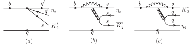
Figure 1: Three different penguin contributions to $\overline{B}\to\overline{K}_{2}^{*}\eta^{(^{\prime})}$. Fig. 1(a) is induced by the penguin operators $O_{3,5,7,9}$.

For $\overline{B}\to\overline{K}_{2}^{*}\eta^{(^{\prime})}$ decays, there exist three different penguin contributions as depicted in Fig. 1: (i) $b\to sq\bar{q}\to s\eta_{q}$, (ii) $b\to ss\bar{s}\to s\eta_{s}$, and (iii) $b\to sq\bar{q}\to q\bar{K}_{2}^{*}$, corresponding to Figs. 1(a), 1(b) and 1(c), respectively. The dominant contributions come from Figs. 1(b) and 1(c). Since the relative sign of the $\eta_{s}$ state with respect to the $\eta_{q}$ is negative for the $\eta$ and positive for the $\eta^{\prime}$ (see Eq. (202)), it is evident that the interference between Figs. 1(b) and 1(c) is destructive for $K^{*}_{2}\eta$ and constructive for $K_{2}^{*}\eta^{\prime}$. This explains why $K_{2}^{*}\eta^{\prime}$ has a rate larger than $K_{2}^{*}\eta$. It was known that the predicted rates in naive factorization are too small by one order of magnitude, of order $1.0\times 10^{-6}$ for ${\cal B}(\overline{B}^{0}\to\bar{K}_{2}^{*0}\eta)$ and $2.5\times 10^{-6}$ for ${\cal B}(\overline{B}^{0}\to\bar{K}_{2}^{*0}\eta^{\prime})$ Munoz ; Cheng:2010sn . One reason is that the factorizable contribution to Fig. 1(c) vanishes in the naive factorization approach. The rates of $K_{2}^{*}\eta^{(^{\prime})}$ are greatly enhanced in QCDF owing to the large power corrections from penguin annihilation and the sizable nonfactorizable contributions to Fig. 1(c).

From Tables 5 and 6 we see that the predicted branching fractions for penguin-dominated $B\to TP$ decays in QCDF are larger than those of Kim:2003 and Munoz by one to two orders of magnitude through the aforementioned two mechanisms for enhancement, while the predicted rates in QCDF are consistent with Kim:2003 for the leading tree-dominated modes such as $a_{2}^{0}\pi^{-},a_{2}^{+}\pi^{-},f_{2}\pi^{-}$. Note that the branching fractions of $B^{-}\to\bar{K}_{2}^{*0}\pi^{-}$ and $\overline{B}^{0}\to K_{2}^{*-}\pi^{+}$ vanish in naive factorization, while experimentally it is $(5.6^{+2.2}_{-1.4})\times 10^{-6}$ for the former. The QCDF calculation indicates that the nonfactorizable contributions arising from vertex, penguin and spectator corrections are sizable to account for the data.

Just as $\overline{B}\to a_{0}\pi$ with $a_{0}=a_{0}(980)$ or $a_{0}(1450)$ and $\overline{B}\to b_{1}(1235)\pi$ decays, we see from Table 6 that for $\overline{B}\to a_{2}(1320)\pi$ decays, the $a_{2}^{-}\pi^{+}$ and $a_{2}^{-}\pi^{0}$ modes are highly suppressed relative to $a_{2}^{+}\pi^{-}$ and $a_{2}^{0}\pi^{-}$, respectively. Since (see Appendix B)

$${\cal A}_{\bar{B}^{0}\to a_{2}^{-}\pi^{+}} \propto \sum_{p=u,c}V_{pb}V^{*}_{pd}\left[\delta_{pu}\,\alpha_{1}+\alpha_{4}^{p}\right]\overline{X}^{(\overline{B}\pi,a_{2})},$$

$${\cal A}_{\bar{B}^{0}\to a_{2}^{+}\pi^{-}} \propto \sum_{p=u,c}V_{pb}V^{*}_{pd}\left[\delta_{pu}\,\alpha_{1}+\alpha_{4}^{p}\right]X^{(\overline{B}a_{2},\pi)},$$ (115)

it is tempting to argue that $\Gamma(\overline{B}^{0}\to a_{2}^{+}\pi^{-})\gg\Gamma(\overline{B}^{0}\to a_{2}^{-}\pi^{+})$ is a natural consequence of naive factorization as the tensor meson cannot be created from the $V-A$ current. However, the suppression of $a_{2}^{-}\pi^{+}$ relative to $a_{2}^{+}\pi^{-}$ in QCDF stems from a different reasoning. The amplitude $\overline{X}^{(\overline{B}\pi,a_{2})}$ does not vanish in QCDF owing to the nonfactorizable corrections. Indeed, $\overline{X}^{(\overline{B}\pi,a_{2})}=0.80$ and $X^{(\overline{B}a_{2},\pi)}=0.69$ are numerically comparable. Therefore, one may wonder how to see the aforementioned suppression ? The key is the quantity $N_{i}(M_{2})$ appearing in the expression for the effective parameter $a_{i}$ [see Eq. (65)]. This quantity vanishes for the tensor meson [cf Eq. (III)]. As a result, the parameter $a_{1}(\pi a_{2})$ is not of order unity as it receives contributions only from vertex corrections and hard spectator interactions, both suppressed by factors of $\alpha_{s}/(4\pi)$. Numerically, we have $a_{1}(\pi a_{2})=-0.035+i0.014$ . By contrast, $a_{1}(a_{2}\pi)$ is of order unity. This explains why $\overline{B}^{0}\to a_{2}^{+}\pi^{-}$ has a rate greater than $a_{2}^{-}\pi^{+}$ and why $B^{-}\to a_{2}^{-}\pi^{0}$ is suppressed relative to $a_{2}^{0}\pi^{-}$. The same pattern also occurs in $\overline{B}\to a_{2}\rho$ decays, see Table 8.

The branching fractions of $B\to a_{2}\eta^{(^{\prime})}$ of order $10^{-7}$ in QCDF are in sharp contrast to the predictions of Munoz , ranging from $25\times 10^{-6}$ to $70\times 10^{-6}$ (see Table 6). It seems to us that it is extremely unlikely that the rate of $a_{2}^{-}\eta^{(^{\prime})}$ can be greater than $a_{2}^{-}\pi^{0}$ by four orders of magnitude as claimed in Munoz . It appears that the former should be slightly smaller than the latter in rates. This can be tested in the future. It is also interesting to notice that while $\overline{B}\to\bar{K}_{2}^{*}K$ decays are very suppressed in naive factorization, their branching fractions are a few $\times 10^{-7}$ in QCDF. Finally, it is worth remarking that $\overline{B}^{0}\to K_{2}^{*+}K^{-}$ and $\overline{B}^{0}\to K_{2}^{*-}K^{+}$ can only proceed through weak annihilation.

IV.2 $B\to TV$ decays

Branching fractions, direct CP asymmetries and the longitudinal polarization fractions for $B\to TV$ decays are shown in Tables 7 and 8. Thus far only four of the $B\to TV$ decays have been measured: $B^{-}\to K_{2}^{*-}(\phi,\omega)$ and $\overline{B}^{0}\to\overline{K}_{2}^{*0}(\phi,\omega)$. They can be used to fix the penguin annihilation parameters. From Eqs. (181) and (183) we have

$$\sqrt{2}{\cal A}_{B^{-}\to K^{*-}_{2}\omega}^{h} \approx \sqrt{2}{\cal A}_{\overline{B}^{0}\to\overline{K}^{*0}_{2}\omega}^{h}\approx\Bigg{\{}\Big{[}\alpha_{4}^{p,h}+\beta_{3}^{p,h}\Big{]}\overline{X}^{(\overline{B}\omega,\overline{K}^{*}_{2})}_{h}+\Big{[}2\alpha_{3}^{p,h}\Big{]}X^{(\overline{B}\overline{K}^{*}_{2},\omega)}_{h}\Bigg{\}},$$

$${\cal A}_{B^{-}\to K^{*-}_{2}\phi}^{h} \approx {\cal A}_{\overline{B}^{0}\to\overline{K}^{*0}_{2}\phi}^{h}\approx\Big{[}\alpha_{3}^{p,h}+\alpha_{4}^{p,h}+\beta_{3}^{p,h}+\beta^{p,h}_{3,{\rm EW}}\Big{]}X^{(\overline{B}\overline{K}^{*}_{2},\phi)}_{h}.$$ (116)

Since $\overline{X}^{(\overline{B}\omega,\overline{K}^{*}_{2})}_{0}/X^{(\overline{B}\overline{K}^{*}_{2},\phi)}_{0}=0.56$ , it is expected that ${\cal B}(B^{-}\to K^{*-}_{2}\omega)/{\cal B}(B^{-}\to K^{*-}_{2}\phi)\approx|\overline{X}^{(\overline{B}\omega,\overline{K}^{*}_{2})}_{0}/X^{(\overline{B}\overline{K}^{*}_{2},\phi)}_{0}|^{2}/2\approx 0.15$ , provided that the penguin-annihilation parameters are the same for $K_{2}^{*}\omega$ and $K_{2}^{*}\phi$, i.e. $\rho_{A}^{K_{2}^{*}\omega}=\rho_{A}^{\phi K_{2}^{*}}$ and likewise for $\phi_{A}$. However, it is the other way around experimentally: the rate of $K_{2}^{*}\omega$ is larger than that of $K_{2}^{*}\phi$. Since in the $B\to VV$ sector, ${\cal B}(B^{-}\to K^{*-}\omega)/{\cal B}(B^{-}\to K^{*-}\phi)\approx 0.3$ HFAG , it is thus puzzling as why $K_{2}^{*}\omega$ behaves so differently from $K^{*}\omega$ in terms of branching fractions. It is clear from Eq. (IV.2) that the $B\to K_{2}^{*}\phi$ decay receives penguin annihilation via $\rho_{A}^{TV}$ and $\phi_{A}^{TV}$, while $B\to K_{2}^{*}\omega$ is governed by $\rho_{A}^{VT}$ and $\phi_{A}^{VT}$. Therefore, we should have $\rho_{A}^{VT}\gg\rho_{A}^{TV}$ in order to account for their rates (see Eq. (124) below).

The branching fractions of the tree-dominated modes $a_{2}\phi,~{}f_{2}\phi,~{}f^{\prime}_{2}\phi$ are very small, of order $10^{-9}$ (see Table 8), as they proceed only through QCD and electroweak penguins.

For charmless $\overline{B}\to TV$ decays, it is naively expected that the helicity amplitudes ${\cal A}_{h}$ (helicities $h=0,-,+$ ) for both tree- and penguin-dominated $\overline{B}\to TV$ decays respect the hierarchy pattern

$${\cal A}_{0}:{\cal A}_{-}:{\cal A}_{+}=1:\left({\Lambda_{\rm QCD}\over m_{b}}\right):\left({\Lambda_{\rm QCD}\over m_{b}}\right)^{2}.$$ (117)

Hence, they are dominated by the longitudinal polarization states and satisfy the scaling law, namely Kagan ,

$$f_{T}\equiv 1-f_{L}={\cal O}\left({m^{2}_{V,T}\over m^{2}_{B}}\right),\qquad{f_{\bot}\over f_{\parallel}}=1+{\cal O}\left({m_{V,T}\over m_{B}}\right),$$ (118)

with $f_{L},f_{\bot}$, $f_{\parallel}$ and $f_{T}$ being the longitudinal, perpendicular, parallel and transverse polarization fractions, respectively, defined as

$$f_{\alpha}\equiv\frac{\Gamma_{\alpha}}{\Gamma}=\frac{|{\cal A}_{\alpha}|^{2}}{|{\cal A}_{0}|^{2}+|{\cal A}_{\parallel}|^{2}+|{\cal A}_{\bot}|^{2}},$$ (119)

with $\alpha=L,\parallel,\bot$.

The so-called polarization puzzle in $B\to VV$ decays is the enigma of why the transverse polarization fraction $f_{T}$ in the penguin-dominated channels such as $B\to\phi K^{*},\rho K^{*}$ is comparable to $f_{L}$, namely, $f_{T}/f_{L}\sim 1$. This poses an interesting challenge for any theoretical interpretation. For $B\to TV$ decays, the experimental measurement indicates that $f_{T}/f_{L}\ll 1$ for $B\to\phi K_{2}^{*}(1430)$, whereas $f_{T}/f_{L}\sim 1$ for $B\to\omega K_{2}^{*}(1430)$, even though both are penguin-dominated.

Consider the ratio of negative- and longitudinal-helicity amplitudes

$$\left.{{\cal A}_{-}\over{\cal A}_{0}}\right|_{B^{-}\to K_{2}^{*-}\omega} \approx \left({\alpha_{4}^{c,-}+\beta_{3}^{-}\over\alpha_{4}^{c,0}+\beta_{3}^{0}}\right)_{\omega K_{2}^{*}}\left({{\overline{X}}^{-}_{\omega K_{2}^{*}}\over\overline{X}^{0}_{\omega K_{2}^{*}}}\right),$$

$$\left.{{\cal A}_{-}\over{\cal A}_{0}}\right|_{B^{-}\to K_{2}^{*-}\phi} \approx \left({\alpha_{4}^{c,-}+\beta_{3}^{-}\over\alpha_{4}^{c,0}+\beta_{3}^{0}}\right)_{K_{2}^{*}\phi}\left({X^{-}_{K_{2}^{*}\phi}\over X^{0}_{K_{2}^{*}\phi}}\right).$$ (120)

The longitudinal polarization fraction can be approximated as

$$f_{L}(\omega K_{2}^{*}) \simeq 1-\frac{|\alpha_{4}^{c,-}+\beta_{3}^{-}|^{2}|\overline{X}^{-}_{\omega K_{2}^{*}}|^{2}}{\sum_{h=0,-}|\alpha_{4}^{c,h}+\beta_{3}^{h}|^{2}|\overline{X}^{h}_{\omega K_{2}^{*}}|^{2}},$$

$$f_{L}(K_{2}^{*}\phi) \simeq 1-\frac{|\alpha_{4}^{c,-}+\beta_{3}^{-}|^{2}|X^{-}_{K_{2}^{*}\phi}|^{2}}{\sum_{h=0,-}|\alpha_{4}^{c,h}+\beta_{3}^{h}|^{2}|X^{h}_{K_{2}^{*}\phi}|^{2}}.$$ (121)

We have

$$|\overline{X}_{\omega K_{2}^{*}}^{0}|:|\overline{X}_{\omega K_{2}^{*}}^{-}|:|\overline{X}_{\omega K_{2}^{*}}^{+}|=1:0.51:0.04\,,$$

$$|X_{K_{2}^{*}\phi}^{0}|:|X_{K_{2}^{*}\phi}^{-}|:|X_{K_{2}^{*}\phi}^{+}|=1:0.38:0.06\,.$$ (122)

In the absence of penguin annihilation, we find $f_{L}(\omega K_{2}^{*})\simeq f_{L}(K_{2}^{*}\phi)\approx 0.72$. As we have stressed in Cheng:2008gxa , in the presence of NLO nonfactorizable corrections e.g. vertex, penguin and hard spectator scattering contributions, the parameters $a_{i}^{h}$ are helicity dependent. Although the factorizable helicity amplitudes $X^{0}$, $X^{-}$ and $X^{+}$ or $\overline{X}^{0}$, $\overline{X}^{-}$, $\overline{X}^{+}$ respect the scaling law (117) with $\Lambda_{\rm QCD}/m_{b}$ replaced by $2m_{V,T}/m_{B}$ for the tensor and vector meson productions, one needs to consider the effects of helicity-dependent Wilson coefficients: ${\cal A}_{-}/{\cal A}_{0}=f(a_{i}^{-})X^{-}/[f(a_{i}^{0})X^{0}]$. The constructive (destructive) interference in the negative-helicity (longitudinal-helicity) amplitude of the penguin-dominated $\overline{B}\to TV$ decay will render $f(a_{i}^{-})\gg f(a_{i}^{0})$ so that ${\cal A}_{-}$ is comparable to ${\cal A}_{0}$ and the transverse polarization is enhanced. Indeed, we find $f_{T}(\omega K_{2}^{*})\simeq f_{T}(K_{2}^{*}\phi)\approx 0.28$ . Therefore, when NLO effects are turned on, their corrections on $a_{i}^{-}$ will render the negative helicity amplitude ${\cal A}_{-}(\overline{B}\to\bar{K}_{2}^{*}\phi)$ comparable to the longitudinal one ${\cal A}_{0}(\overline{B}\to\bar{K}_{2}^{*}\phi)$ so that even at the short-distance level, $f_{L}$ for $\overline{B}^{0}\to\bar{K}_{2}^{*}\phi$ is reduced to the level of 70% and likewise for $\overline{B}^{0}\to\bar{K}_{2}^{*}\omega$.

As noticed in passing, penguin annihilation is needed in order to account for the observed rates. This is because, in the absence of power corrections, QCDF predicts too small rates for penguin-dominated $\overline{B}\to TV$ and $VV,VA$ decays. For example, the calculated $\overline{B}\to\bar{K}_{2}^{*}\phi$ rate is too small by a factor of 2.5 and $\overline{B}\to\bar{K}_{2}^{*}\omega$ by two orders of magnitude. We shall rely on power corrections from penguin annihilation to enhance the rates. A nice feature of the $(S-P)(S+P)$ penguin annihilation is that it contributes to ${\cal A}_{0}$ and ${\cal A}_{-}$ with the same order of magnitude Kagan:2004ia

$${\cal A}_{0}^{\rm PA}:{\cal A}_{-}^{\rm PA}:{\cal A}_{+}^{\rm PA}=\left({\Lambda_{\rm QCD}\over m_{b}}{\ln{m_{b}\over\Lambda_{h}}}\right)^{2}:\left({\Lambda_{\rm QCD}\over m_{b}}{\ln{m_{b}\over\Lambda_{h}}}\right)^{2}:\left({\Lambda_{\rm QCD}\over m_{b}}\right)^{4}.$$ (123)

The logarithmic divergences are associated with the limit in which both the $s$ and $\bar{s}$ quarks originating from the gluon are soft Kagan:2004ia . As for the power counting, the annihilation topology is of order $1/m_{b}$ and each remaining factor of $1/m_{b}$ is associated with a quark helicity flip. The fact that ${\cal A}_{-}^{\rm PA}$ and ${\cal A}_{0}^{\rm PA}$ have the same power counting explains why penguin annihilation is helpful to resolve the polarization puzzle. The relative size of ${\cal A}_{-}^{\rm PA}$ and ${\cal A}_{0}^{\rm PA}$ depends mainly on the phase $\phi_{A}$. It turns out that the longitudinal polarization fraction for $B\to K_{2}^{*}\phi$ is quite sensitive to the phase $\phi_{A}^{TV}$, while $f_{L}(\omega K_{2}^{*})$ is not so sensitive to $\phi_{A}^{VT}$. For example, $f_{L}(K_{2}^{*}\phi)=0.88,~{}0.72,~{}0.48$, respectively, for $\phi_{A}^{TV}=-30^{\circ},-45^{\circ},-60^{\circ}$ and $f_{L}(\omega K_{2}^{*})=0.68,~{}0.66,~{}0.64$, respectively, for $\phi_{A}^{VT}=-30^{\circ},-45^{\circ},-60^{\circ}$. Hence, we can use the experimental measurements of $f_{L}$ to fix the phases $\phi_{A}^{VT}$ and $\phi_{A}^{TV}$ and branching fractions to pin down the parameters $\rho_{A}(VT)$ and $\rho_{A}(TV)$:

$$\rho_{A}^{TV}=0.65,\qquad\phi_{A}^{TV}=-33^{\circ},\qquad\rho_{A}^{VT}=1.20,\qquad\phi_{A}^{VT}=-60^{\circ}\,.$$ (124)

It should be stressed that although the experimental observation of the longitudinal polarization in $B\to K_{2}^{*}\phi$ and $B\to K_{2}^{*}\omega$ decays can be accommodated in the QCDF approach, no dynamical explanation is offered for the smallness of $f_{T}(K_{2}^{*}\phi)$ and the sizable $f_{T}(\omega K_{2}^{*})$.

For penguin-dominated $B\to TV$ decays, we find $f_{L}(K_{2}^{*}\rho)\sim f_{L}(K_{2}^{*}\omega)\sim 0.65$ , whereas $f_{L}(f_{2}K^{*})\sim 0.93$ (cf. Table 7). It will be very interesting to measure $f_{L}$ for these modes to test the approach of QCDF. Theoretically, transverse polarization is expected to be small in tree-dominated $\overline{B}\to TV$ decays except for the $a_{2}^{-}\rho^{0},~{}a_{2}^{-}\rho^{+},~{}K_{2}^{*0}K^{*-}$ and $K_{2}^{*0}\bar{K}^{*0}$ modes.

V Conclusions

We have studied in this work the charmless hadronic $B$ decays with a tensor meson in the final state within the framework of QCD factorization. Due to the $G$-parity of the tensor meson, both the chiral-even and chiral-odd two-parton LCDAs of the tensor meson are antisymmetric under the interchange of momentum fractions of the quark and anti-quark in the SU(3) limit. The main results of this work are as follows:

• We have worked out the longitudinal and transverse helicity projection operators for the tensor meson. They are very similar to the projectors for the vector meson. Consequently, the nonfactorizable contributions such as vertex, penguin and hard spectator corrections to $B\to T(P,V)$ decays can be directly obtained from $B\to VP,VV$ ones by making some suitable replacement.

• The factorizable amplitude with a tensor meson emitted vanishes under the factorization hypothesis owing to the fact that a tensor meson cannot be created from the local $V-A$ and tensor currents. As a result, $B^{-}\to\bar{K}_{2}^{*0}\pi^{-}$ and $\overline{B}^{0}\to K_{2}^{*-}\pi^{+}$ vanish in naive factorization. The experimental observation of the former implies the importance of nonfactorizable effects.

• Five different models for $B\to T$ transition form factors were considered. While the predictions of $B\to f_{2}(1270)$ form factors based on large energy effective theory or pQCD are favored by experiment, the covariant light-front quark model or the ISGW2 model for $B\to K_{2}^{*}(1430)$ ones is preferred by the data.

• For penguin-dominated $B\to TP$ and $TV$ decays, the predicted rates in naive factorization are normally too small by one to two orders of magnitude. In QCDF, they are enhanced by the power corrections from penguin annihilation and nonfactorizable contributions.

• There exist three distinct types of penguin contributions to $B\to K_{2}^{*}\eta^{(^{\prime})}$: (i) $b\to sq\bar{q}\to s\eta_{q}$, (ii) $b\to ss\bar{s}\to s\eta_{s}$, and (iii) $b\to sq\bar{q}\to q\bar{K}_{2}^{*}$ with $\eta_{q}=(u\bar{u}+d\bar{d})/\sqrt{2}$ and $\eta_{s}=s\bar{s}$. The dominant effects arise from the last two penguin contributions. The interference, constructive for $K_{2}^{*}\eta^{\prime}$ and destructive for $K_{2}^{*}\eta$ between type-(ii) and type-(iii) diagrams, explains why $\Gamma(B\to K_{2}^{*}\eta^{\prime})\gg\Gamma(B\to K_{2}^{*}\eta)$.

• We use the measured rates of $K_{2}^{*}\omega$ and $K_{2}^{*}\phi$ modes to extract the penguin annihilation parameters $\rho_{A}^{TV}$ and $\rho_{A}^{VT}$ and the observed longitudinal polarization fractions $f_{L}(K_{2}^{*}\omega)$ and $f_{L}(K_{2}^{*}\phi)$ to fix the phases $\phi_{A}^{VT}$ and $\phi_{A}^{TV}$. The unexpectedly large rate of $B\to K_{2}^{*}\omega$ relative to $B\to K_{2}^{*}\phi$ implies that $\rho_{A}^{VT}\gg\rho_{A}^{VT}$. However, it may be hard to offer more intuitive understanding for the large disparity between $\rho_{A}^{TV}$ and $\rho_{A}^{VT}$ in magnitude.

• The experimental observation that $f_{T}/f_{L}\ll 1$ for $B\to\phi K_{2}^{*}(1430)$, whereas $f_{T}/f_{L}\sim 1$ for $B\to\omega K_{2}^{*}(1430)$, can be accommodated in QCDF, but cannot be dynamically explained at first place. For penguin-dominated $B\to TV$ decays, we find $f_{L}(K_{2}^{*}\rho)\sim f_{L}(K_{2}^{*}\omega)\sim 0.65$ and $f_{L}(K^{*}f_{2})\sim 0.93$. It will be of great interest to measure $f_{L}$ for these modes to test QCDF. Theoretically, transverse polarization is expected to be small in tree-dominated $\overline{B}\to TV$ decays except for the $a_{2}^{-}\rho^{0},~{}a_{2}^{-}\rho^{+},~{}K_{2}^{*0}K^{*-}$ and $K_{2}^{*0}\bar{K}^{*0}$ modes.

• For tree-dominated decays, their rates are usually very small except for the $a_{2}^{0}(\pi^{-},\rho^{-}),~{}a_{2}^{+}(\pi^{-},\rho^{-})$ and $f_{2}(\pi^{-},\rho^{-})$ modes with branching fractions of order $10^{-6}$ or even bigger.

Acknowledgments

One of us (H.Y.C.) wishes to thank C.N. Yang Institute for Theoretical Physics at SUNY Stony Brook for its hospitality. This work was supported in part by the National Center for Theoretical Sciences and the National Science Council of R.O.C. under Grant Nos. NSC97-2112-M-008-002-MY3 and NSC99-2112-M-003-005-MY3.

Appendix A Form factors in the ISGW2 quark model

Consider the transition $B\to T$ in the ISGW2 quark model ISGW2 , where the tensor meson $T$ has the quark content $q_{1}\bar{q}_{2}$ with $\bar{q}_{2}$ being the spectator quark. We begin with the definition ISGW2

$$F_{n}=\left({\tilde{m}_{T}\over\tilde{m}_{B}}\right)^{1/2}\left({\beta_{B}\beta_{T}\over\beta_{BT}^{2}}\right)^{n/2}\left[1+{1\over 18}r^{2}(t_{m}-t)\right]^{-3},$$ (125)

where

$$r^{2}={3\over 4m_{b}m_{1}}+{3m_{2}^{2}\over 2\bar{m}_{B}\bar{m}_{T}\beta_{BT}^{2}}+{1\over\bar{m}_{B}\bar{m}_{T}}\left({16\over 33-2n_{f}}\right)\ln\left[{\alpha_{s}(\mu_{\rm QM})\over\alpha_{s}(m_{1})}\right],$$ (126)

$\tilde{m}$ is the sum of the meson’s constituent quarks’ masses, $\bar{m}$ is the hyperfine-averaged mass (for example, $\bar{m}_{B}={3\over 4}m_{B^{*}}+{1\over 4}m_{B}$), $t_{m}=(m_{B}-m_{T})^{2}$ is the maximum momentum transfer, and

$$\mu_{\pm}=\left({1\over m_{1}}\pm{1\over m_{b}}\right)^{-1},$$ (127)

with $m_{1}$ and $m_{2}$ being the masses of the quarks $q_{1}$ and $\bar{q}_{2}$, respectively. In Eq. (125), the values of the parameters $\beta_{B}$ and $\beta_{T}$ are available in ISGW2 and $\beta_{BT}^{2}={1\over 2}(\beta_{B}^{2}+\beta_{T}^{2})$.

The form factors defined by Eq. (17) have the following expressions in the ISGW2 model:

$$h = {m_{2}\over 2\sqrt{2}\tilde{m}_{B}\beta_{B}}\left[{1\over m_{1}}-{m_{2}\beta^{2}_{B}\over 2\mu_{-}\tilde{m}_{T}\beta^{2}_{BT}}\right]F_{5}^{(h)},$$

$$k = {m_{2}\over\sqrt{2}\beta_{B}}(1+\tilde{\omega})F_{5}^{(k)},$$

$$b_{+}+b_{-} = {m_{2}^{2}\over 4\sqrt{2}m_{q}m_{b}\tilde{m}_{B}\beta_{B}}\,{\beta^{2}_{T}\over\beta^{2}_{BT}}\left(1-{m_{2}\over 2\tilde{m}_{B}}{\beta^{2}_{T}\over\beta^{2}_{BT}}\right)F_{5}^{(b_{+}+b_{-})},$$ (128)

$$b_{+}-b_{-} = -{m_{2}\over\sqrt{2}m_{b}\tilde{m}_{T}\beta_{B}}\left[1-{m_{2}m_{b}\over 2\mu_{+}\tilde{m}_{B}}{\beta^{2}_{T}\over\beta^{2}_{BT}}+{m_{2}\over 4m_{q}}{\beta^{2}_{T}\over\beta^{2}_{BT}}\left(1-{m_{2}\over 2\tilde{m}_{B}}{\beta^{2}_{T}\over\beta^{2}_{BT}}\right]\right)F_{5}^{(b_{+}-b_{-})},$$

where

$$F_{5}^{(h)}=F_{5}\left({\bar{m}_{B}\over\tilde{m}_{B}}\right)^{-3/2}\left({\bar{m}_{T}\over\tilde{m}_{T}}\right)^{-1/2},$$

$$F_{5}^{(k)}=F_{5}\left({\bar{m}_{B}\over\tilde{m}_{B}}\right)^{-1/2}\left({\bar{m}_{T}\over\tilde{m}_{T}}\right)^{1/2},$$

$$F_{5}^{(b_{+}+b_{-})}=F_{5}\left({\bar{m}_{B}\over\tilde{m}_{B}}\right)^{-5/2}\left({\bar{m}_{T}\over\tilde{m}_{T}}\right)^{1/2},$$

$$F_{5}^{(b_{+}-b_{-})}=F_{5}\left({\bar{m}_{B}\over\tilde{m}_{B}}\right)^{-3/2}\left({\bar{m}_{T}\over\tilde{m}_{T}}\right)^{-1/2},$$ (129)

and

$$\tilde{\omega}-1=\,{t_{m}-t\over 2\bar{m}_{B}\bar{m}_{T}}.$$ (130)

In the original version of the ISGW model ISGW , the function $F_{n}$ has a different expression in its $(t_{m}-t)$ dependence:

$$F_{n}=\left({\tilde{m}_{T}\over\tilde{m}_{B}}\right)^{1/2}\left({\beta_{B}\beta_{T}\over\beta_{BT}^{2}}\right)^{n/2}{\rm exp}\left\{-{m_{2}\over 4\tilde{m}_{B}\tilde{m}_{T}}\,{t_{m}-t\over\kappa^{2}\beta_{BT}^{2}}\right\},$$ (131)

where $\kappa=0.7$ is the relativistic correction factor. The form factors are then given by

$$h = {m_{2}\over 2\sqrt{2}\tilde{m}_{B}\beta_{B}}\left[{1\over m_{1}}-{m_{2}\over 2\tilde{m}_{T}\mu_{-}}{\beta^{2}_{B}\over\beta^{2}_{BT}}\right]F_{5},$$

$$k = {m_{2}\over\sqrt{2}\beta_{B}}F_{5},$$

$$b_{+} = -{m_{2}\over 2\sqrt{2}m_{b}\tilde{m}_{T}\beta_{B}}\left[1-{m_{2}m_{b}\over 2\mu_{+}\tilde{m}_{B}}{\beta^{2}_{T}\over\beta^{2}_{BT}}+{m_{2}m_{b}\over 4\tilde{m}_{B}\mu_{-}}{\beta^{2}_{T}\over\beta^{2}_{BT}}\left(1-{m_{2}\over 2\tilde{m}_{B}}{\beta^{2}_{T}\over\beta^{2}_{BT}}\right)\right]F_{5}.$$ (132)

Note that the expressions in Eq. (A) in the ISGW2 model allow one to determine the form factor $b_{-}$, which vanishes in the ISGW model.

Appendix B Decay amplitudes

The coefficients of the flavor operators $\alpha_{i}^{p,(h)}$ can be expressed in terms of $a_{i}^{p,(h)}$ in the following:

$$\alpha_{1}(M_{1}M_{2}) = a_{1}(M_{1}M_{2})\,,$$

$$\alpha_{2}(M_{1}M_{2}) = a_{2}(M_{1}M_{2})\,,$$

$$\alpha_{3}^{p}(M_{1}M_{2}) = \left\{\begin{array}[]{cl}a_{3}^{p}(M_{1}M_{2})-a_{5}^{p}(M_{1}M_{2})&\quad\mbox{for~{}}M_{1}M_{2}=TP\,,\\ a_{3}^{p}(M_{1}M_{2})+a_{5}^{p}(M_{1}M_{2})&\quad\mbox{for~{}}M_{1}M_{2}=PT\,,\end{array}\right.$$ (135)

$$\alpha_{4}^{p}(M_{1}M_{2}) = \left\{\begin{array}[]{cl}a_{4}^{p}(M_{1}M_{2})-r_{\chi}^{M_{2}}\,a_{6}^{p}(M_{1}M_{2})&\quad\mbox{for~{}}M_{1}M_{2}=TP\\ a_{4}^{p}(M_{1}M_{2})+r_{\chi}^{M_{2}}\,a_{6}^{p}(M_{1}M_{2})&\quad\mbox{for~{}}M_{1}M_{2}=PT\,,\end{array}\right.$$ (138)

$$\alpha_{3,\rm EW}^{p}(M_{1}M_{2}) = \left\{\begin{array}[]{cl}a_{9}^{p}(M_{1}M_{2})-a_{7}^{p}(M_{1}M_{2})&\quad\mbox{for~{}}M_{1}M_{2}=TP\,,\\ a_{9}^{p}(M_{1}M_{2})+a_{7}^{p}(M_{1}M_{2})&\quad\mbox{for~{}}M_{1}M_{2}=PT\,,\end{array}\right.$$ (141)

$$\alpha_{4,\rm EW}^{p}(M_{1}M_{2}) = \left\{\begin{array}[]{cl}a_{10}^{p}(M_{1}M_{2})-r_{\chi}^{M_{2}}\,a_{8}^{p}(M_{1}M_{2})&\quad\mbox{for~{}}M_{1}M_{2}=TP\,,\\ a_{10}^{p}(M_{1}M_{2})+r_{\chi}^{M_{2}}\,a_{8}^{p}(M_{1}M_{2})&\quad\mbox{for~{}}M_{1}M_{2}=PT\,,\end{array}\right.$$ (144)

for $\overline{B}\to TP$ decays, and

$$\alpha_{1}^{h}(M_{1}M_{2}) = a_{1}^{h}(M_{1}M_{2})\,,$$

$$\alpha_{2}^{h}(M_{1}M_{2}) = a_{2}^{h}(M_{1}M_{2})\,,$$

$$\alpha_{3}^{p,h}(M_{1}M_{2}) = a_{3}^{p,h}(M_{1}M_{2})+a_{5}^{p,h}(M_{1}M_{2}),$$ (145)

$$\alpha_{4}^{p,h}(M_{1}M_{2}) = a_{4}^{p,h}(M_{1}M_{2})-r_{\chi}^{M_{2}}\,a_{6}^{p,h}(M_{1}M_{2})\,,$$

$$\alpha_{3,\rm EW}^{p,h}(M_{1}M_{2}) = a_{9}^{p,h}(M_{1}M_{2})+a_{7}^{p,h}(M_{1}M_{2})\,,$$

$$\alpha_{4,\rm EW}^{p,h}(M_{1}M_{2}) = a_{10}^{p,h}(M_{1}M_{2})-r_{\chi}^{M_{2}}\,a_{8}^{p,h}(M_{1}M_{2}),$$

for $\overline{B}\to TV$ decays with $(M_{1}M_{2})\equiv(TV)$ or $(VT)$. It should be noted that the order of the arguments of $\alpha_{i}^{p}(M_{1}M_{2})$ and $a_{i}^{p}(M_{1}M_{2})$ is relevant. The chiral factor $r_{\chi}^{M}$ is given by

$$r_{\chi}^{\pi,K}(\mu)=\frac{2m_{\pi,K}^{2}}{m_{b}(\mu)\,(m_{q_{1}}+m_{q_{2}})(\mu)}\,,\quad r_{\chi}^{\eta_{q,s}^{(\prime)}}(\mu)=\frac{h_{q,s}}{f_{q,s}^{(\prime)}\,m_{b}(\mu)\,m_{q,s}(\mu)}$$ (146)

for the pseudoscalar mesons,

$$r_{\chi}^{V}(\mu)=\frac{2m_{V}}{m_{b}(\mu)}\,\frac{f_{V}^{\perp}(\mu)}{f_{V}}\,$$ (147)

for the vector meson, and

$$r_{\chi}^{T}(\mu)=\frac{2m_{T}}{m_{b}(\mu)}\,\frac{f_{T}^{\perp}(\mu)}{f_{T}}\,$$ (148)

for the tensor meson. See Appendix D for further discussions on the parameters $h_{q,s}$ and $f_{q,s}^{(\prime)}$.

In the following decay amplitudes, the order of the arguments of $\alpha_{i}^{p(,h)}(M_{1}M_{2})$ and $\beta_{i}^{p(,h)}(M_{1}M_{2})$ is consistent with the order of the arguments of $X_{(h)}^{(\overline{B}M_{1},M_{2})}$ or $\overline{X}_{(h)}^{(\overline{B}M_{1},M_{2})}$, where

$$\beta_{i}^{p}(TP)=\frac{-if_{B}f_{T}f_{P}}{X^{(\overline{B}T,P)}}b_{i}^{p},\quad\beta_{i}^{p}(PT)=\frac{-if_{B}f_{T}f_{P}}{\overline{X}^{(\overline{B}P,T)}}b_{i}^{p},~{}~{}{\rm for}~{}TP~{}{\rm modes},$$ (149)

$$\beta_{i}^{p,h}(TV)=\frac{if_{B}f_{T}f_{V}}{X_{h}^{(\overline{B}T,V)}}b_{i}^{p,h},\quad\beta_{i}^{p,h}(VT)=\frac{if_{B}f_{T}f_{V}}{\overline{X}_{h}^{(\overline{B}V,T)}}b_{i}^{p,h},~{}~{}{\rm for}~{}TV~{}{\rm modes}.$$ (150)

The decay amplitudes for $\overline{B}\to TP,TV$ are summarized as follows:

B.1 $\overline{B}\to TP$ decays

B.1.1 Decay amplitudes with $\Delta S=0$:

$$\sqrt{2}\,{\cal A}_{B^{-}\to f_{2}\pi^{-}} = \frac{G_{F}}{\sqrt{2}}\sum_{p=u,c}\lambda_{p}^{(d)}$$ (151)

$$\times\Bigg{\{}\Big{[}\delta_{pu}\,(\alpha_{2}+\beta_{2})+2\alpha_{3}^{p}+\alpha_{4}^{p}+\frac{1}{2}\alpha_{3,{\rm EW}}^{p}-\frac{1}{2}\alpha_{4,{\rm EW}}^{p}+\beta_{3}^{p}+\beta_{3,{\rm EW}}^{p}\Big{]}\overline{X}^{(\overline{B}\pi,f_{2}^{q})}$$

$$+\sqrt{2}\left[\alpha_{3}^{p}-\frac{1}{2}\alpha_{3,{\rm EW}}^{p}\right]\overline{X}^{(\overline{B}\pi,f_{2}^{s})}$$

$$+\left[\delta_{pu}\,(\alpha_{1}+\beta_{2})+\alpha_{4}^{p}+\alpha_{4,{\rm EW}}^{p}+\beta_{3}^{p}+\beta_{3,{\rm EW}}^{p}\right]X^{(\overline{B}f_{2}^{q},\pi)}\Bigg{\}},$$

$$-2\,{\cal A}_{\overline{B}^{0}\to f_{2}\pi^{0}} = \frac{G_{F}}{\sqrt{2}}\sum_{p=u,c}\lambda_{p}^{(d)}\Bigg{\{}\Big{[}\delta_{pu}\,(\alpha_{2}-\beta_{1})+2\alpha_{3}^{p}+\alpha_{4}^{p}+\frac{1}{2}\alpha_{3,{\rm EW}}^{p}-\frac{1}{2}\alpha_{4,{\rm EW}}^{p}$$ (152)

$$\hskip 28.45274pt+\,\beta_{3}^{p}-\frac{1}{2}\beta_{3,{\rm EW}}^{p}-\frac{3}{2}\beta_{4,{\rm EW}}^{p}\Big{]}\overline{X}^{(\overline{B}\pi,f_{2}^{q})}+\sqrt{2}\left[\alpha_{3}^{p}-\frac{1}{2}\alpha_{3,{\rm EW}}^{p}\right]\overline{X}^{(\overline{B}\pi,f_{2}^{s})}$$

$$+\left[\delta_{pu}\,(-\alpha_{2}-\beta_{1})+\alpha_{4}^{p}-\frac{3}{2}\alpha_{3,{\rm EW}}^{p}-\frac{1}{2}\alpha_{4,{\rm EW}}^{p}\right.$$

$$\hskip 28.45274pt\,\left.+\beta_{3}^{p}-\frac{1}{2}\beta_{3,{\rm EW}}^{p}-\frac{3}{2}\beta_{4,{\rm EW}}^{p}\right]X^{(\overline{B}f_{2}^{q},\pi)}\Bigg{\}},$$

$$2\,{\cal A}_{\bar{B}^{0}\to f_{2}\eta} = \frac{G_{F}}{\sqrt{2}}\sum_{p=u,c}\lambda_{p}^{(d)}\Bigg{\{}\Big{[}\delta_{pu}\,(\alpha_{2}+\beta_{1})+2\alpha_{3}^{p}+\alpha_{4}^{p}+\frac{1}{2}\alpha_{3,{\rm EW}}^{p}-\frac{1}{2}\alpha_{4,{\rm EW}}^{p}$$ (153)

$$\hskip 28.45274pt+\,\beta_{3}^{p}+2\beta_{4}^{p}-\frac{1}{2}\beta_{3,{\rm EW}}^{p}+\frac{1}{2}\beta_{4,{\rm EW}}^{p}\Big{]}X^{(\overline{B}f_{2}^{q},\eta_{q})}$$

$$+ \sqrt{2}\left[\alpha_{3}^{p}-\frac{1}{2}\alpha_{3,{\rm EW}}^{p}\right]X^{(\overline{B}f_{2}^{q},\eta_{s})}+\sqrt{2}\left[\delta_{pc}\,\alpha_{2}+\alpha_{3}^{p}\right]X^{(\overline{B}f_{2}^{q},\eta_{c})}-2if_{B}f_{2}^{s}f_{\eta}^{s}\left[b_{4}^{p}-\frac{1}{2}b_{4,{\rm EW}}^{p}\right]_{f_{2}^{s}\eta_{s}}$$

$$+ \Big{[}\delta_{pu}\,(\alpha_{2}+\beta_{1})+2\alpha_{3}^{p}+\alpha_{4}^{p}+\frac{1}{2}\alpha_{3,{\rm EW}}^{p}-\frac{1}{2}\alpha_{4,{\rm EW}}^{p}$$

$$\hskip 28.45274pt+\,\beta_{3}^{p}+2\beta_{4}^{p}-\frac{1}{2}\beta_{3,{\rm EW}}^{p}+\frac{1}{2}\beta_{4,{\rm EW}}^{p}\Big{]}\overline{X}^{(\overline{B}\eta_{q},f_{2}^{q})}$$

$$+ \sqrt{2}\left[\alpha_{3}^{p}-\frac{1}{2}\alpha_{3,{\rm EW}}^{p}\right]\overline{X}^{(\overline{B}\eta_{q},f_{2}^{s})}-2if_{B}f_{2}^{s}f_{\eta}^{s}\left[b_{4}^{p}-\frac{1}{2}b_{4,{\rm EW}}^{p}\right]_{\eta_{s}f_{2}^{s}}\Bigg{\}},$$

the amplitudes for $\overline{B}\to f_{2}\eta^{\prime}$ can be obtained from $\overline{B}\to f_{2}\eta$ with the replacement $(f_{2},\eta)\to(f_{2},\eta^{\prime})$,

$$\sqrt{2}\,{\cal A}_{B^{-}\to a_{2}^{0}\pi^{-}} = \frac{G_{F}}{\sqrt{2}}\sum_{p=u,c}\lambda_{p}^{(d)}\Bigg{\{}\left[\delta_{pu}\,(\alpha_{2}-\beta_{2})-\alpha_{4}^{p}+\frac{3}{2}\alpha_{3,{\rm EW}}^{p}+\frac{1}{2}\alpha_{4,{\rm EW}}^{p}-\beta_{3}^{p}-\beta_{3,{\rm EW}}^{p}\right]\overline{X}^{(\overline{B}\pi,a_{2})}$$ (154)

$$+\left[\delta_{pu}\,(\alpha_{1}+\beta_{2})+\alpha_{4}^{p}+\alpha_{4,{\rm EW}}^{p}+\beta_{3}^{p}+\beta_{3,{\rm EW}}^{p}\right]X^{(\overline{B}a_{2},\pi)}\Bigg{\}},$$

$$\sqrt{2}\,{\cal A}_{B^{-}\to a_{2}^{-}\pi^{0}} = \frac{G_{F}}{\sqrt{2}}\sum_{p=u,c}\lambda_{p}^{(d)}\Bigg{\{}\left[\delta_{pu}\,(\alpha_{2}-\beta_{2})-\alpha_{4}^{p}+\frac{3}{2}\alpha_{3,{\rm EW}}^{p}+\frac{1}{2}\alpha_{4,{\rm EW}}^{p}-\beta_{3}^{p}-\beta_{3,{\rm EW}}^{p}\right]X^{(\overline{B}a_{2},\pi)}$$ (155)

$$+ \left[\delta_{pu}\,(\alpha_{1}+\beta_{2})+\alpha_{4}^{p}+\alpha_{4,{\rm EW}}^{p}+\beta_{3}^{p}+\beta_{3,{\rm EW}}^{p}\right]\overline{X}^{(\overline{B}\pi,a_{2})}\Bigg{\}},$$

$${\cal A}_{\bar{B}^{0}\to a_{2}^{-}\pi^{+}} = \frac{G_{F}}{\sqrt{2}}\sum_{p=u,c}\lambda_{p}^{(d)}\Bigg{\{}\left[\delta_{pu}\,\alpha_{1}+\alpha_{4}^{p}+\alpha_{4,{\rm EW}}^{p}+\beta_{3}^{p}+\beta_{4}^{p}-\frac{1}{2}\beta_{3,{\rm EW}}^{p}-\frac{1}{2}\beta_{4,{\rm EW}}^{p}\right]\overline{X}^{(\overline{B}\pi,a_{2})}$$ (156)

$$+\left[\delta_{pu}\,\beta_{1}+\beta_{4}^{p}+\beta_{4,{\rm EW}}^{p}\right]X^{(\overline{B}a_{2},\pi)}\Bigg{\}},$$

$${\cal A}_{\bar{B}^{0}\to a_{2}^{+}\pi^{-}} = \frac{G_{F}}{\sqrt{2}}\sum_{p=u,c}\lambda_{p}^{(d)}\Bigg{\{}\left[\delta_{pu}\,\alpha_{1}+\alpha_{4}^{p}+\alpha_{4,{\rm EW}}^{p}+\beta_{3}^{p}+\beta_{4}^{p}-\frac{1}{2}\beta_{3,{\rm EW}}^{p}-\frac{1}{2}\beta_{4,{\rm EW}}^{p}\right]X^{(\overline{B}a_{2},\pi)}$$ (157)

$$+ \left[\delta_{pu}\,\beta_{1}+\beta_{4}^{p}+\beta_{4,{\rm EW}}^{p}\right]\overline{X}^{(\overline{B}\pi,a_{2})}\Bigg{\}},$$

$$-2\,{\cal A}_{\bar{B}^{0}\to a_{2}^{0}\pi^{0}} = \frac{G_{F}}{\sqrt{2}}\sum_{p=u,c}\lambda_{p}^{(d)}\Bigg{\{}\Big{[}\delta_{pu}\,(\alpha_{2}-\beta_{1})-\alpha_{4}^{p}+\frac{3}{2}\alpha_{3,{\rm EW}}^{p}+\frac{1}{2}\alpha_{4,{\rm EW}}^{p}-\beta_{3}^{p}-2\beta_{4}^{p}$$ (158)

$$\hskip 28.45274pt+\,\frac{1}{2}\beta_{3,{\rm EW}}^{p}-\frac{1}{2}\beta_{4,{\rm EW}}^{p}\Big{]}\overline{X}^{(\overline{B}\pi,a_{2})}$$

$$+\Big{[}\delta_{pu}\,(\alpha_{2}-\beta_{1})-\alpha_{4}^{p}+\frac{3}{2}\alpha_{3,{\rm EW}}^{p}+\frac{1}{2}\alpha_{4,{\rm EW}}^{p}-\beta_{3}^{p}-2\beta_{4}^{p}$$

$$\hskip 28.45274pt+\,\frac{1}{2}\beta_{3,{\rm EW}}^{p}-\frac{1}{2}\beta_{4,{\rm EW}}^{p}\Big{]}X^{(\overline{B}a_{2},\pi)}\Bigg{\}},$$

$$\sqrt{2}\,{\cal A}_{B^{-}\to a_{2}^{-}\eta^{(\prime)}} = \frac{G_{F}}{\sqrt{2}}\sum_{p=u,c}\lambda_{p}^{(d)}\Bigg{\{}\bigg{[}\delta_{pu}\,(\alpha_{2}+\beta_{2})+2\alpha_{3}^{p}+\alpha_{4}^{p}+\frac{1}{2}\alpha_{3,{\rm EW}}^{p}$$ (159)

$$-\frac{1}{2}\alpha_{4,{\rm EW}}^{p}+\beta_{3}^{p}+\beta_{3,{\rm EW}}^{p}\bigg{]}X^{(\overline{B}a_{2},\eta_{q}^{(\prime)})}$$

$$+\left[\delta_{pu}\,(\alpha_{1}+\beta_{2})+\alpha_{4}^{p}+\alpha_{4,{\rm EW}}^{p}+\beta_{3}^{p}+\beta_{3,{\rm EW}}^{p}\right]\overline{X}^{(\overline{B}\eta_{q}^{(\prime)},a_{2})}$$

$$+\sqrt{2}\left[\alpha_{3}^{p}-\frac{1}{2}\alpha_{3,{\rm EW}}^{p}\right]X^{(\overline{B}a_{2},\eta_{s}^{(\prime)})}+\sqrt{2}\left[\delta_{pc}\,\alpha_{2}+\alpha_{3}^{p}\right]X^{(\overline{B}a_{2},\eta_{c}^{(\prime)})}\Bigg{\}},$$

$$-2\,{\cal A}_{\bar{B}^{0}\to a_{2}^{0}\eta^{(\prime)}} = \frac{G_{F}}{\sqrt{2}}\sum_{p=u,c}\lambda_{p}^{(d)}\Bigg{\{}\Big{[}\delta_{pu}\,(\alpha_{2}-\beta_{1})+2\alpha_{3}^{p}+\alpha_{4}^{p}+\frac{1}{2}\alpha_{3,{\rm EW}}^{p}-\frac{1}{2}\alpha_{4,{\rm EW}}^{p}$$ (160)

$$+\beta_{3}^{p}-\,\frac{1}{2}\beta_{3,{\rm EW}}^{p}-\frac{3}{2}\beta_{4,{\rm EW}}^{p}\Big{]}X^{(\overline{B}a_{2},\eta_{q}^{(\prime)})}$$

$$+\Big{[}\delta_{pu}\,(-\alpha_{2}-\beta_{1})+\alpha_{4}^{p}-\frac{3}{2}\alpha_{3,{\rm EW}}^{p}-\frac{1}{2}\alpha_{4,{\rm EW}}^{p}$$

$$+\beta_{3}^{p}-\,\frac{1}{2}\beta_{3,{\rm EW}}^{p}-\frac{3}{2}\beta_{4,{\rm EW}}^{p}\Big{]}\overline{X}^{(\overline{B}\eta_{q}^{(\prime)},a_{2})}$$

$$+\sqrt{2}\left[\alpha_{3}^{p}-\frac{1}{2}\alpha_{3,{\rm EW}}^{p}\right]X^{(\overline{B}a_{2},\eta_{s}^{(\prime)})}+\sqrt{2}\left[\delta_{pc}\,\alpha_{2}+\alpha_{3}^{p}\right]X^{(\overline{B}a_{2},\eta_{c}^{(\prime)})}\Bigg{\}}\,,$$

$${\cal A}_{B^{-}\to K^{*-}_{2}K^{0}} = \frac{G_{F}}{\sqrt{2}}\sum_{p=u,c}\lambda_{p}^{(d)}\Big{[}\delta_{pu}\beta_{2}+\alpha_{4}^{p}-\frac{1}{2}\alpha_{4,{\rm EW}}^{p}+\beta_{3}^{p}+\beta^{p}_{3,{\rm EW}}\Big{]}X^{(\overline{B}\overline{K}_{2}^{*},K)},$$ (161)

$${\cal A}_{B^{-}\to K^{*0}_{2}K^{-}} = \frac{G_{F}}{\sqrt{2}}\sum_{p=u,c}\lambda_{p}^{(d)}\Big{[}\delta_{pu}\beta_{2}+\alpha_{4}^{p}-\frac{1}{2}\alpha_{4,{\rm EW}}^{p}+\beta_{3}^{p}+\beta^{p}_{3,{\rm EW}}\Big{]}\overline{X}^{(\overline{B}\overline{K},K_{2}^{*})},$$ (162)

$${\cal A}_{\overline{B}^{0}\to K^{*-}_{2}K^{+}} = \frac{G_{F}}{\sqrt{2}}\sum_{p=u,c}\lambda_{p}^{(d)}\Bigg{\{}\Big{[}\delta_{pu}\beta_{1}+\beta_{4}^{p}+\beta^{p}_{4,{\rm EW}}\Big{]}X^{(\overline{B}\overline{K}_{2}^{*},K)}$$ (163)

$$-icf_{B}f_{K_{2}^{*}}f_{K}\left[b_{4}^{p}-{1\over 2}b^{p}_{4,{\rm EW}}\right]_{KK_{2}^{*}}\Bigg{\}},$$

$${\cal A}_{\overline{B}^{0}\to K^{*+}_{2}K^{-}} = \frac{G_{F}}{\sqrt{2}}\sum_{p=u,c}\lambda_{p}^{(d)}\Bigg{\{}\Big{[}\delta_{pu}\beta_{1}+\beta_{4}^{p}+\beta^{p}_{4,{\rm EW}}\Big{]}\overline{X}^{(\overline{B}\overline{K},K_{2}^{*})}$$ (164)

$$-icf_{B}f_{K_{2}^{*}}f_{K}\left[b_{4}^{p}-{1\over 2}b^{p}_{4,{\rm EW}}\right]_{K_{2}^{*}K}\Bigg{\}},$$

$${\cal A}_{\overline{B}^{0}\to\overline{K}^{*0}_{2}K^{0}} = \frac{G_{F}}{\sqrt{2}}\sum_{p=u,c}\lambda_{p}^{(d)}\Bigg{\{}\Big{[}\alpha_{4}^{p}-{1\over 2}\alpha^{p}_{4,{\rm EW}}+\beta^{p}_{3}+\beta_{4}^{p}-{1\over 2}\beta^{p}_{3,{\rm EW}}-{1\over 2}\beta^{p}_{4,{\rm EW}}\Big{]}X^{(\overline{B}\overline{K}_{2}^{*},K)},$$ (165)

$$-icf_{B}f_{K_{2}^{*}}f_{K}\left[b_{4}^{p}-{1\over 2}b^{p}_{4,{\rm EW}}\right]_{K\overline{K}_{2}^{*}}\Bigg{\}},$$

$${\cal A}_{\overline{B}^{0}\to K^{*0}_{2}\overline{K}^{0}} = \frac{G_{F}}{\sqrt{2}}\sum_{p=u,c}\lambda_{p}^{(d)}\Bigg{\{}\Big{[}\alpha_{4}^{p}-{1\over 2}\alpha^{p}_{4,{\rm EW}}+\beta^{p}_{3}+\beta_{4}^{p}-{1\over 2}\beta^{p}_{3,{\rm EW}}-{1\over 2}\beta^{p}_{4,{\rm EW}}\Big{]}\overline{X}^{(\overline{B}\bar{K},K_{2}^{*})},$$ (166)

$$-icf_{B}f_{K_{2}^{*}}f_{K}\left[b_{4}^{p}-{1\over 2}b^{p}_{4,{\rm EW}}\right]_{K^{*}_{2}\overline{K}}\Bigg{\}},$$

with $c=1$.

B.1.2 Decay amplitudes with $\Delta S=1$

$$\sqrt{2}\,{\cal A}_{B^{-}\to f_{2}K^{-}} = \frac{G_{F}}{\sqrt{2}}\sum_{p=u,c}\lambda_{p}^{(s)}\Bigg{\{}\left[\delta_{pu}\,\alpha_{2}+2\alpha_{3}^{p}+\frac{1}{2}\alpha_{3,{\rm EW}}^{p}\right]\overline{X}^{(\overline{B}\bar{K},f_{2}^{q})}$$ (167)

$$+\sqrt{2}\Big{[}\delta_{pu}\,\beta_{2}+\alpha_{3}^{p}+\alpha_{4}^{p}-\frac{1}{2}\alpha_{3,{\rm EW}}^{p}-\frac{1}{2}\alpha_{4,{\rm EW}}^{p}+\beta_{3}^{p}+\beta_{3,{\rm EW}}^{p}\Big{]}\overline{X}^{(\overline{B}\bar{K},f_{2}^{s})}$$

$$+ \left[\delta_{pu}\,(\alpha_{1}+\beta_{2})+\alpha_{4}^{p}+\alpha_{4,{\rm EW}}^{p}+\beta_{3}^{p}+\beta_{3,{\rm EW}}^{p}\right]X^{(\overline{B}f_{2}^{q},\bar{K})},$$

$$\sqrt{2}\,{\cal A}_{\bar{B}^{0}\to f_{2}K^{0}} = \frac{G_{F}}{\sqrt{2}}\sum_{p=u,c}\lambda_{p}^{(s)}\Bigg{\{}\left[\delta_{pu}\,\alpha_{2}+2\alpha_{3}^{p}+\frac{1}{2}\alpha_{3,{\rm EW}}^{p}\right]\overline{X}^{(\overline{B}\bar{K},f_{2}^{q})}$$ (168)

$$+ \sqrt{2}\Big{[}\alpha_{3}^{p}+\alpha_{4}^{p}-\frac{1}{2}\alpha_{3,{\rm EW}}^{p}-\frac{1}{2}\alpha_{4,{\rm EW}}^{p}+\beta_{3}^{p}-\frac{1}{2}\beta_{3,{\rm EW}}^{p}\Big{]}\overline{X}^{(\overline{B}\bar{K},f_{2}^{s})}$$

$$+ \left[\alpha_{4}^{p}-\frac{1}{2}\alpha_{4,{\rm EW}}^{p}+\beta_{3}^{p}-\frac{1}{2}\beta_{3,{\rm EW}}^{p}\right]X^{(\overline{B}f_{2}^{q},\bar{K})},$$

$$\sqrt{2}{\cal A}_{B^{-}\to a_{2}^{0}K^{-}} = \frac{G_{F}}{\sqrt{2}}\sum_{p=u,c}\lambda_{p}^{(s)}\Bigg{\{}\Big{[}\delta_{pu}(\alpha_{1}+\beta_{2})+\alpha_{4}^{p}+\alpha_{4,{\rm EW}}^{p}+\beta_{3}^{p}+\beta^{p}_{3,{\rm EW}}\Big{]}X^{(\overline{B}a_{2},\overline{K})}$$ (169)

$$+\Big{[}\delta_{pu}\alpha_{2}+{3\over 2}\alpha^{p}_{3,{\rm EW}}\Big{]}\overline{X}^{(\overline{B}\overline{K},a_{2})}\Bigg{\}},$$

$${\cal A}_{B^{-}\to a_{2}^{-}K^{0}} = \frac{G_{F}}{\sqrt{2}}\sum_{p=u,c}\lambda_{p}^{(s)}\Big{[}\delta_{pu}\beta_{2}+\alpha_{4}^{p}-\frac{1}{2}\alpha_{4,{\rm EW}}^{p}+\beta_{3}^{p}+\beta^{p}_{3,{\rm EW}}\Big{]}X^{(\overline{B}a_{2},\overline{K})},$$ (170)

$${\cal A}_{\overline{B}^{0}\to a_{2}^{+}K^{-}} = \frac{G_{F}}{\sqrt{2}}\sum_{p=u,c}\lambda_{p}^{(s)}\Big{[}\delta_{pu}\alpha_{1}^{h}+\alpha_{4}^{p}+\alpha_{4,{\rm EW}}^{p}+\beta_{3}^{p}-{1\over 2}\beta^{p}_{3,{\rm EW}}\Big{]}X^{(\overline{B}a_{2},\overline{K})},$$ (171)

$$\sqrt{2}{\cal A}_{\overline{B}^{0}\to a_{2}^{0}K^{0}} = \frac{G_{F}}{\sqrt{2}}\sum_{p=u,c}\lambda_{p}^{(s)}\Bigg{\{}\Big{[}-\alpha_{4}^{p}+{1\over 2}\alpha_{4,{\rm EW}}^{p}-\beta_{3}^{p}+{1\over 2}\beta^{p}_{3,{\rm EW}}\Big{]}X^{(\overline{B}a_{2},\overline{K})}$$ (172)

$$+ \Big{[}\delta_{pu}\alpha_{2}+{3\over 2}\alpha^{p}_{3,{\rm EW}}\Big{]}\overline{X}^{(\overline{B}\overline{K},a_{2})}\Bigg{\}},$$

$$\sqrt{2}\,{\cal A}_{B^{-}\to K_{2}^{*-}\eta^{(\prime)}} = \frac{G_{F}}{\sqrt{2}}\sum_{p=u,c}\lambda_{p}^{(s)}\Bigg{\{}\left[\delta_{pu}\,\alpha_{2}+2\alpha_{3}^{p}+\frac{1}{2}\alpha_{3,{\rm EW}}^{p}\right]X^{(\overline{B}\overline{K}_{2}^{*},\eta^{(\prime)}_{q})}$$ (173)

$$+ \sqrt{2}\Big{[}\delta_{pu}\,\beta_{2}+\alpha_{3}^{p}+\alpha_{4}^{p}-\frac{1}{2}\alpha_{3,{\rm EW}}^{p}-\frac{1}{2}\alpha_{4,{\rm EW}}^{p}+\beta_{3}^{p}+\beta_{3,{\rm EW}}^{p}\Big{]}X^{(\overline{B}\overline{K}_{2}^{*},\eta^{(\prime)}_{s})}$$

$$+ \sqrt{2}\left[\delta_{pc}\,\alpha_{2}+\alpha_{3}^{p}\right]X^{(\overline{B}\overline{K}_{2}^{*},\eta^{(\prime)}_{c})}$$

$$+ \left[\delta_{pu}\,(\alpha_{1}+\beta_{2})+\alpha_{4}^{p}+\alpha_{4,{\rm EW}}^{p}+\beta_{3}^{p}+\beta_{3,{\rm EW}}^{p}\right]X^{(\overline{B}\eta^{(\prime)}_{q},\overline{K}_{2}^{*})}\Bigg{\}},$$

$$\sqrt{2}\,{\cal A}_{\bar{B}^{0}\to\bar{K}_{2}^{*0}\eta^{(\prime)}} = \frac{G_{F}}{\sqrt{2}}\sum_{p=u,c}\lambda_{p}^{(s)}\Bigg{\{}\left[\delta_{pu}\,\alpha_{2}+2\alpha_{3}^{p}+\frac{1}{2}\alpha_{3,{\rm EW}}^{p}\right]X^{(\overline{B}\overline{K}_{2}^{*},\eta^{(\prime)}_{q})}$$ (174)

$$+ \sqrt{2}\Big{[}\alpha_{3}^{p}+\alpha_{4}^{p}-\frac{1}{2}\alpha_{3,{\rm EW}}^{p}-\frac{1}{2}\alpha_{4,{\rm EW}}^{p}+\beta_{3}^{p}-\frac{1}{2}\beta_{3,{\rm EW}}^{p}\Big{]}X^{(\overline{B}\overline{K}_{2}^{*},\eta^{(\prime)}_{s})}$$

$$+ \sqrt{2}\left[\delta_{pc}\,\alpha_{2}+\alpha_{3}^{p}\right]X^{(\overline{B}\overline{K}_{2}^{*},\eta^{(\prime)}_{c})}$$

$$+ \left[\alpha_{4}^{p}-\frac{1}{2}\alpha_{4,{\rm EW}}^{p}+\beta_{3}^{p}-\frac{1}{2}\beta_{3,{\rm EW}}^{p}\right]\overline{X}^{(\overline{B}\eta^{(\prime)}_{q},\overline{K}_{2}^{*})}\Bigg{\}},$$

and the amplitudes for $\overline{B}\to\overline{K}_{2}^{*}\pi$ can be obtained from $\overline{B}\to\overline{K}a_{2}$ with the replacement $(\overline{K},a_{2})\to(\overline{K}_{2}^{*},\pi)$.

B.2 $\overline{B}\to TV$ decays

B.2.1 Decay amplitudes with $\Delta S=0$:

The amplitudes for $\overline{B}\to f_{2}\rho$ can be obtained from $\overline{B}\to f_{2}\pi$ with the replacement $(f_{2},\pi)\to(f_{2},\rho)$,

$$2\,{\cal A}_{\bar{B}^{0}\to f_{2}\omega} = \frac{G_{F}}{\sqrt{2}}\sum_{p=u,c}\lambda_{p}^{(d)}\Bigg{\{}\Big{[}\delta_{pu}\,(\alpha_{2}^{h}+\beta_{1}^{h})+2\alpha_{3}^{p,h}+\alpha_{4}^{p,h}+\frac{1}{2}\alpha_{3,{\rm EW}}^{p,h}-\frac{1}{2}\alpha_{4,{\rm EW}}^{p,h}$$ (175)

$$\hskip 8.5359pt+\,\beta_{3}^{p,h}+2\beta_{4}^{p,h}-\frac{1}{2}\beta_{3,{\rm EW}}^{p,h}+\frac{1}{2}\beta_{4,{\rm EW}}^{p,h}\Big{]}X^{(\overline{B}f_{2}^{q},\omega)}$$

$$+ \Big{[}\delta_{pu}\,(\alpha_{2}^{h}+\beta_{1}^{h})+2\alpha_{3}^{p,h}+\alpha_{4}^{p,h}+\frac{1}{2}\alpha_{3,{\rm EW}}^{p,h}-\frac{1}{2}\alpha_{4,{\rm EW}}^{p,h}+\,\beta_{3}^{p,h}+2\beta_{4}^{p,h}$$

$$\hskip 8.5359pt-\frac{1}{2}\beta_{3,{\rm EW}}^{p,h}+\frac{1}{2}\beta_{4,{\rm EW}}^{p,h}\Big{]}\overline{X}^{(\overline{B}\omega,f_{2}^{q})}+\sqrt{2}\left[\alpha_{3}^{p,h}-\frac{1}{2}\alpha_{3,{\rm EW}}^{p,h}\right]\overline{X}^{(\overline{B}\omega,f_{2}^{s})}\Bigg{\}},$$

$$2\,{\cal A}_{\bar{B}^{0}\to f_{2}\phi} = \frac{G_{F}}{\sqrt{2}}\sum_{p=u,c}\lambda_{p}^{(d)}\Bigg{\{}\sqrt{2}\left[\alpha_{3}^{p,h}-\frac{1}{2}\alpha_{3,{\rm EW}}^{p,h}\right]X^{(\overline{B}f_{2}^{q},\phi)}+2if_{B}f_{2}^{s}f_{\phi}\left[b_{4}^{p,h}-\frac{1}{2}b_{4,{\rm EW}}^{p,h}\right]_{f_{2}^{s}\phi}$$ (176)

$$+ 2if_{B}f_{2}^{s}f_{\phi}\left[b_{4}^{p,h}-\frac{1}{2}b_{4,{\rm EW}}^{p,h}\right]_{\phi f_{2}^{s}}\Bigg{\}},$$

the amplitudes for $\overline{B}\to a_{2}\rho$ can be obtained from $\overline{B}\to a_{2}\pi$ with the replacement $(a_{2},\pi)\to(a_{2},\rho)$,

$$\sqrt{2}\,{\cal A}_{B^{-}\to a_{2}^{-}\omega}^{h} = \frac{G_{F}}{\sqrt{2}}\sum_{p=u,c}\lambda_{p}^{(d)}\Bigg{\{}\bigg{[}\delta_{pu}\,(\alpha_{2}^{h}+\beta_{2}^{h})+2\alpha_{3}^{p,h}+\alpha_{4}^{p,h}+\frac{1}{2}\alpha_{3,{\rm EW}}^{p,h}$$ (177)

$$-\frac{1}{2}\alpha_{4,{\rm EW}}^{p,h}+\beta_{3}^{p,h}+\beta_{3,{\rm EW}}^{p,h}\bigg{]}X^{(\overline{B}a_{2},\omega)}_{h}$$

$$+ \left[\delta_{pu}\,(\alpha_{1}^{h}+\beta_{2}^{h})+\alpha_{4}^{p,h}+\alpha_{4,{\rm EW}}^{p,h}+\beta_{3}^{p,h}+\beta_{3,{\rm EW}}^{p,h}\right]\overline{X}^{(\overline{B}\omega,a_{2})}_{h}\Bigg{\}},$$

$$-2\,{\cal A}_{\bar{B}^{0}\to a_{2}^{0}\omega}^{h} = \frac{G_{F}}{\sqrt{2}}\sum_{p=u,c}\lambda_{p}^{(d)}\Bigg{\{}\Big{[}\delta_{pu}\,(\alpha_{2}^{h}-\beta_{1}^{h})+2\alpha_{3}^{p,h}+\alpha_{4}^{p,h}+\frac{1}{2}\alpha_{3,{\rm EW}}^{p,h}-\frac{1}{2}\alpha_{4,{\rm EW}}^{p,h}$$ (178)

$$\hskip 28.45274pt+\beta_{3}^{p,h}-\,\frac{1}{2}\beta_{3,{\rm EW}}^{p,h}-\frac{3}{2}\beta_{4,{\rm EW}}^{p,h}\Big{]}X^{(\overline{B}a_{2},\omega)}_{h}$$

$$\hskip 28.45274pt+\Big{[}\delta_{pu}\,(-\alpha_{2}^{h}-\beta_{1}^{h})+\alpha_{4}^{p,h}-\frac{3}{2}\alpha_{3,{\rm EW}}^{p,h}-\frac{1}{2}\alpha_{4,{\rm EW}}^{p,h}$$

$$\hskip 28.45274pt+\beta_{3}^{p,h}-\,\frac{1}{2}\beta_{3,{\rm EW}}^{p,h}-\frac{3}{2}\beta_{4,{\rm EW}}^{p,h}\Big{]}\overline{X}^{(\overline{B}\omega,a_{2})}_{h}\Bigg{\}}\,,$$

$${\cal A}_{B^{-}\to a_{2}^{-}\phi}^{h} = \frac{G_{F}}{\sqrt{2}}\sum_{p=u,c}\lambda_{p}^{(d)}\Bigg{\{}\left[\alpha_{3}^{p,h}-\frac{1}{2}\alpha_{3,{\rm EW}}^{p,h}\right]X^{(\overline{B}a_{2},\phi)}_{h}\Bigg{\}}\,,$$ (179)

$$-\sqrt{2}\,{\cal A}_{\bar{B}^{0}\to a_{2}^{0}\phi}^{h} = \frac{G_{F}}{\sqrt{2}}\sum_{p=u,c}\lambda_{p}^{(d)}\Bigg{\{}\left[\alpha_{3}^{p,h}-\frac{1}{2}\alpha_{3,{\rm EW}}^{p,h}\right]X^{(\overline{B}a_{2},\phi)}_{h}\Bigg{\}}\,,$$ (180)

and the amplitudes for $\overline{B}\to\overline{K}_{2}^{*}K^{*}$ can be obtained from $\overline{B}\to\overline{K}_{2}^{*}K$ with the replacement $(\overline{K}^{*}_{2},K)\to(\overline{K}_{2}^{*},K^{*})$ and $c=-1$.

B.2.2 Decay amplitudes with $\Delta S=1$

The amplitudes for $\overline{B}\to f_{2}\overline{K}^{*}$ can be obtained from $\overline{B}\to f_{2}\overline{K}$ with the replacement $(f_{2},\overline{K})\to(f_{2},\overline{K}^{*})$, and the ones for $\overline{B}\to\overline{K}_{2}^{*}\rho$ and $\overline{B}\to\overline{K}^{*}a_{2}$ can be obtained from $\overline{B}\to\overline{K}a_{2}$ with the replacement $(\overline{K},a_{2})\to(\overline{K}_{2}^{*},\rho)$ and $(\overline{K},a_{2})\to(\overline{K}^{*},a_{2})$, respectively,

$$\sqrt{2}{\cal A}_{B^{-}\to K^{*-}_{2}\omega}^{h} = \frac{G_{F}}{\sqrt{2}}\sum_{p=u,c}\lambda_{p}^{(s)}\Bigg{\{}\Big{[}\delta_{pu}(\alpha_{1}^{h}+\beta_{2}^{h})+\alpha_{4}^{p,h}+\alpha_{4,{\rm EW}}^{p,h}+\beta_{3}^{p,h}+\beta^{p,h}_{3,{\rm EW}}\Big{]}\overline{X}^{(\overline{B}\omega,\overline{K}^{*}_{2})}_{h}$$ (181)

$$+ \Big{[}\delta_{pu}\alpha_{2}^{h}+2\alpha_{3}^{p,h}+{1\over 2}\alpha^{p,h}_{3,{\rm EW}}\Big{]}X^{(\overline{B}\overline{K}^{*}_{2},\omega)}_{h}\Bigg{\}},$$

$$\sqrt{2}{\cal A}_{\overline{B}^{0}\to\overline{K}^{*0}_{2}\omega}^{h} = \frac{G_{F}}{\sqrt{2}}\sum_{p=u,c}\lambda_{p}^{(s)}\Bigg{\{}\Big{[}\alpha_{4}^{p,h}-{1\over 2}\alpha_{4,{\rm EW}}^{p,h}+\beta_{3}^{p,h}-{1\over 2}\beta^{p,h}_{3,{\rm EW}}\Big{]}\overline{X}^{(\overline{B}\omega,\overline{K}^{*}_{2})}_{h}$$ (182)

$$+ \Big{[}\delta_{pu}\alpha_{2}^{h}+2\alpha_{3}^{p,h}+{1\over 2}\alpha^{p,h}_{3,{\rm EW}}\Big{]}X^{(\overline{B}\overline{K}^{*}_{2},\omega)}_{h}\Bigg{\}},$$

$${\cal A}_{B^{-}\to K^{*-}_{2}\phi}^{h} = \frac{G_{F}}{\sqrt{2}}\sum_{p=u,c}\lambda_{p}^{(s)}\Big{[}\delta_{pu}\beta_{2}^{h}+\alpha_{3}^{p,h}+\alpha_{4}^{p,h}-{1\over 2}\alpha_{3,{\rm EW}}^{p,h}$$ (183)

$$-{1\over 2}\alpha_{4,{\rm EW}}^{p,h}+\beta_{3}^{p,h}+\beta^{p,h}_{3,{\rm EW}}\Big{]}X^{(\overline{B}\overline{K}^{*}_{2},\phi)}_{h},$$

$${\cal A}_{\overline{B}^{0}\to\overline{K}^{*0}_{2}\phi}^{h} = \frac{G_{F}}{\sqrt{2}}\sum_{p=u,c}\lambda_{p}^{(s)}\Big{[}\alpha_{3}^{p,h}+\alpha_{4}^{p,h}-{1\over 2}\alpha_{3,{\rm EW}}^{p,h}-{1\over 2}\alpha_{4,{\rm EW}}^{p,h}$$ (184)

$$+\beta_{3}^{p,h}-{1\over 2}\beta^{p,h}_{3,{\rm EW}}\Big{]}X^{(\overline{B}\overline{K}^{*}_{2},\phi)}_{h}.$$

Appendix C Explicit expressions of annihilation amplitudes

The general expressions of the helicity-dependent annihilation amplitudes are given in Eqs. (90)-(99). They can be further simplified by considering the asymptotic distribution amplitudes for $\Phi_{V},\Phi_{v},\Phi_{T}$ and $\Phi_{t}$:

$$\Phi^{V}_{\parallel,\perp}(u)=6u\bar{u},\qquad\Phi_{v}(u)=3(2u-1),$$

$$\Phi^{T}_{\parallel,\bot}(u)=30u\bar{u}(2u-1),\qquad\Phi_{t}(u)=5(1-6u+6u^{2}),$$

$$\Phi^{M}_{+}(u)=\int^{1}_{u}dv{\Phi^{M}_{\parallel}(v)\over v},\qquad\Phi^{M}_{-}(u)=\int^{u}_{0}dv{\Phi^{M}_{\parallel}(v)\over\bar{v}}.$$ (185)

We find

$$A_{3}^{f,\,0}(V\,T) \approx -30\sqrt{2\over 3}\pi\alpha_{s}\left[\left(6{X_{A}^{0}}^{2}-23X_{A}^{0}+22\right)r_{\chi}^{V}+{3\over 2}(2X_{A}^{0}-1)(X_{A}^{0}-3)r_{\chi}^{T}\right],$$ (186)

$$A_{3}^{f,\,-}(V\,T) \approx -{10\over\sqrt{2}}\pi\alpha_{s}\left[\left(6{X_{A}^{-}}^{2}-23X_{A}^{-}+17\right)\frac{m_{T}}{m_{V}}r_{\chi}^{V}+9(2X_{A}^{-}-3)(X_{A}^{-}-2)\frac{m_{V}}{m_{T}}r_{\chi}^{T}\right],$$ (187)

$$A_{3}^{f,\,0}(T\,V) = -A_{3}^{f,\,0}(V\,T),\qquad A_{3}^{f,\,-}(T\,V)=-A_{3}^{f,\,-}(V\,T),$$ (188)

$$A_{3}^{i,\,0}(V\,T) \approx 30\sqrt{2\over 3}\pi\alpha_{s}\left[-3\left({X_{A}^{0}}^{2}-4X_{A}^{0}-4+\pi^{2}\right)r_{\chi}^{V}+\frac{3}{2}\left({X_{A}^{0}}^{2}-2X_{A}^{0}-6+\frac{\pi^{2}}{3}\right)r_{\chi}^{T}\right],$$ (189)

$$A_{3}^{i,\,-}(V\,T) \approx -{30\over\sqrt{2}}\pi\alpha_{s}\Bigg{[}-\left({X_{A}^{-}}^{2}-2X_{A}^{-}-2\right)\frac{m_{T}}{m_{V}}r_{\chi}^{V}+\left(3{X_{A}^{-}}^{2}-12X_{A}^{-}+2\pi^{2}\right)\frac{m_{V}}{m_{T}}r_{\chi}^{T}\Bigg{]},$$ (190)

$$A_{3}^{i,\,0}(T\,V) = A_{3}^{i,\,0}(V\,T),\qquad A_{3}^{i,\,-}(T\,V)=A_{3}^{i,\,-}(V\,T),$$ (191)

$$A_{1}^{i,\,0}(V\,T) \approx 30\sqrt{2\over 3}\pi\alpha_{s}\left[3X_{A}^{0}+4-\pi^{2}+{3\over 2}(X_{A}^{0}-3)(X_{A}^{0}-2)r_{\chi}^{V}r_{\chi}^{T}\right],$$ (192)

$$A_{1}^{i,\,0}(T\,V) \approx -30\sqrt{2\over 3}\pi\alpha_{s}\left[X_{A}^{0}+29-3\pi^{2}+{3\over 2}(X_{A}^{0}-3)(X_{A}^{0}-2)r_{\chi}^{V}r_{\chi}^{T}\right],$$ (193)

$$A_{2}^{i,\,0}(V\,T) = -A_{1}^{i,\,0}(T\,V),\qquad A_{2}^{i,\,0}(T\,V)=-A_{1}^{i,\,0}(V\,T),$$ (194)

for $TV$ modes, and

$$A_{3}^{f}(P\,T) \approx \sqrt{2\over 3}\pi\alpha_{s}\left[10X_{A}(6X_{A}-11)r_{\chi}^{P}+45(2X_{A}-1)(X_{A}-3)r_{\chi}^{T}\right],$$ (195)

$$A_{3}^{i}(P\,T) \approx 30\sqrt{2\over 3}\pi\alpha_{s}\left[\left({X_{A}}^{2}-4X_{A}+4+\frac{\pi^{2}}{3}\right)r_{\chi}^{P}+\frac{3}{2}\left({X_{A}}^{2}-2X_{A}-6+\frac{\pi^{2}}{3}\right)r_{\chi}^{T}\right],$$ (196)

$$A_{1}^{i}(P\,T) \approx 10\sqrt{2\over 3}\pi\alpha_{s}\left[3(3X_{A}+4-\pi^{2})+{3\over 2}X_{A}(X_{A}-3)r_{\chi}^{P}r_{\chi}^{T}\right],$$ (197)

$$A_{1}^{i}(T\,P) \approx -10\sqrt{2\over 3}\pi\alpha_{s}\left[3(X_{A}+29-3\pi^{2})+{3\over 2}X_{A}(X_{A}-3)r_{\chi}^{P}r_{\chi}^{T}\right],$$ (198)

$$A_{3}^{f}(P\,T) = A_{3}^{f}(T\,P),\qquad A_{3}^{i}(T\,P)=A_{3}^{i}(P\,T),$$ (199)

$$A_{2}^{i}(T\,P) = A_{1}^{i}(P\,T),\qquad A_{2}^{i}(P\,T)=A_{1}^{i}(T\,P),$$ (200)

for $TP$ modes. As pointed out in Cheng:2008gxa , since the annihilation contributions $A_{1,2}^{i,\pm}$ are suppressed by a factor of $m_{1}m_{2}/m_{B}^{2}$ relative to other terms, in numerical analysis we will consider only the annihilation contributions due to $A_{3}^{f,0}$, $A_{3}^{f,-}$, $A_{1,2,3}^{i,0}$ and $A_{3}^{i,-}$.

The logarithmic divergences that occurred in weak annihilation in above equations are described by the variable $X_{A}$

$$\int_{0}^{1}{du\over u}\to X_{A},\qquad\int_{0}^{1}du{\ln u\over u}\to-{1\over 2}(X_{A})^{2}.$$ (201)

Following BBNS , these variables are parameterized in Eq. (100) in terms of the unknown real parameters $\rho_{A}$ and $\phi_{A}$. For simplicity, we shall assume in practical calculations that $X_{A}^{h}$ are helicity independent, $X_{A}^{-}=X_{A}^{+}=X_{A}^{0}$.

Appendix D The $\eta-\eta^{\prime}$ system

For the $\eta$ and $\eta^{\prime}$ particles, it is more convenient to work with the flavor states $q\bar{q}\equiv(u\bar{u}+d\bar{d})/\sqrt{2}$, $s\bar{s}$ and $c\bar{c}$ labeled by the $\eta_{q}$, $\eta_{s}$ and $\eta_{c}^{0}$, respectively. Neglecting the small mixing with $\eta_{c}^{0}$, we write

$$\left(\begin{array}[]{c}|\eta\rangle\\ |\eta^{\prime}\rangle\end{array}\right)=\left(\begin{array}[]{ccc}\cos\phi&-\sin\phi\\ \sin\phi&\cos\phi\end{array}\right)\left(\begin{array}[]{c}|\eta_{q}\rangle\\ |\eta_{s}\rangle\end{array}\right)\;,$$ (202)

where $\phi=(39.3\pm 1.0)^{\circ}$ FKS is the $\eta-\eta^{\prime}$ mixing angle in the $\eta_{q}$ and $\eta_{s}$ flavor basis. Decay constants $f^{q}_{\eta^{(^{\prime})}}$, $f_{\eta^{(^{\prime})}}^{s}$ and $f_{\eta^{(^{\prime})}}^{c}$ are defined by

$$\langle 0|\bar{q}\gamma_{\mu}\gamma_{5}q|\eta^{(^{\prime})}\rangle=i{1\over\sqrt{2}}f_{\eta^{(^{\prime})}}^{q}p_{\mu},\quad\langle 0|\bar{s}\gamma_{\mu}\gamma_{5}s|\eta^{(^{\prime})}\rangle=if_{\eta^{(^{\prime})}}^{s}p_{\mu},\quad\langle 0|\bar{c}\gamma_{\mu}\gamma_{5}c|\eta^{(^{\prime})}\rangle=if_{\eta^{(^{\prime})}}^{c}p_{\mu},$$ (203)

while the widely studied decay constants $f_{q}$ and $f_{s}$ are defined as FKS

$$\langle 0|\bar{q}\gamma^{\mu}\gamma_{5}q|\eta_{q}\rangle = \frac{i}{\sqrt{2}}\,f_{q}\,p^{\mu}\;,\qquad\langle 0|\bar{s}\gamma^{\mu}\gamma_{5}s|\eta_{s}\rangle=if_{s}\,p^{\mu}\;.$$ (204)

The ansatz made by Feldmann, Kroll and Stech (FKS) FKS is that the decay constants in the quark flavor basis follow the same pattern of $\eta-\eta^{\prime}$ mixing given in Eq. (202)

$$\left(\begin{array}[]{cc}f_{\eta}^{q}&f_{\eta}^{s}\\ f_{\eta^{\prime}}^{q}&f_{\eta^{\prime}}^{s}\end{array}\right)=\left(\begin{array}[]{ccc}\cos\phi&-\sin\phi\\ \sin\phi&\cos\phi\end{array}\right)\left(\begin{array}[]{cc}f_{q}&0\\ 0&f_{s}\end{array}\right).$$ (211)

Empirically, this ansatz works very well FKS . Theoretically, it has been shown recently that this assumption can be justified in the large-$N_{c}$ approach Mathieu:2010ss .

It is useful to consider the matrix elements of pseudoscalar densities BenekeETA

$$2m_{q}\langle 0|\bar{q}\gamma_{5}q|\eta^{(^{\prime})}\rangle={i\over\sqrt{2}}h^{q}_{\eta^{(^{\prime})}},\qquad 2m_{s}\langle 0|\bar{s}\gamma_{5}s|\eta^{(^{\prime})}\rangle={i}h^{s}_{\eta^{(^{\prime})}},$$ (212)

and define the parameters $h_{q}$ and $h_{s}$ in analogue to $f_{q}$ and $f_{s}$

$$2m_{q}\langle 0|\bar{q}\gamma_{5}q|\eta_{q}\rangle=\frac{i}{\sqrt{2}}\,h_{q}\;,\qquad 2m_{s}\langle 0|\bar{s}\gamma_{5}s|\eta_{s}\rangle = ih_{s}\;,$$ (213)

and relate them to $h_{\eta,\eta^{\prime}}^{q,s}$ by the similar FKS ansatz as in Eq. (211).

In this work, we shall follow BN to use

$$h_{\eta}^{q}=0.0013\,{\rm GeV}^{3},\quad h_{\eta}^{s}=-0.0555\,{\rm GeV}^{3},\quad h_{\eta^{\prime}}^{q}=0.0011\,{\rm GeV}^{3},\quad h_{\eta^{\prime}}^{s}=0.068\,{\rm GeV}^{3},$$

$$f_{\eta}^{q}=109\,{\rm MeV},\qquad~{}~{}f_{\eta}^{s}=-111\,{\rm MeV},\qquad~{}f_{\eta^{\prime}}^{q}=89\,{\rm MeV},\qquad\quad~{}f_{\eta^{\prime}}^{s}=136\,{\rm MeV},$$

$$f_{\eta}^{c}=-2.3\,{\rm MeV},\qquad f_{\eta^{\prime}}^{c}=-5.8\,{\rm MeV},\qquad~{}~{}m_{\eta_{q}}=741\,{\rm MeV},\qquad m_{\eta_{s}}=802\,{\rm MeV},$$ (214)

where we have used the perturbative result fetac

$$f_{\eta^{(^{\prime})}}^{c}=-{m_{\eta^{(^{\prime})}}^{2}\over 12m_{c}^{2}}\,{f_{\eta^{(^{\prime})}}^{q}\over\sqrt{2}}.$$ (215)

The form factors for $B\to\eta^{(^{\prime})}$ transitions obtained in QCD sum rules are Ball:Beta

$$F^{B\eta}_{0,1}(0) = 0.229\pm 0.024\pm 0.011,$$

$$F^{B\eta^{\prime}}_{0,1}(0) = 0.188\pm 0.002B_{2}^{g}\pm 0.019\pm 0.009,$$ (216)

where the flavor-singlet contribution to the $B\to\eta^{(^{\prime})}$ form factors is characterized by the parameter $B_{2}^{g}$, a gluonic Gegenbauer moment. It appears that the singlet contribution to the form factor is small unless $B_{2}^{g}$ assumes extreme values $\sim 40$ Ball:Beta . Using the relation

$$F^{B\eta}_{0,1}=F^{B\eta_{q}}_{0,1}\cos\phi,\quad F^{B\eta^{\prime}}_{0,1}=F^{B\eta_{q}}_{0,1}\sin\phi,$$ (217)

we obtain $F^{B\eta_{q}}_{0,1}(0)=0.296\pm 0.028$ as shown in Table 4. The momentum dependence of the form factor can be found in Ball:Beta .

References

- (1) P. del Amo Sanchez et al. [BABAR Collaboration], Phys. Rev. D 82, 011502 (2010) [arXiv:1004.0240 [hep-ex]].
- (2) B. Aubert et al. [BABAR Collaboration], Phys. Rev. Lett. 97, 201802 (2006) [arXiv:hep-ex/0608005].
- (3) B. Aubert et al. [BABAR Collaboration], Phys. Rev. D 79, 052005 (2009) [arXiv:0901.3703 [hep-ex]].
- (4) B. Aubert et al. [BABAR Collaboration], Phys. Rev. D 78, 012004 (2008) [arXiv:0803.4451 [hep-ex]].
- (5) A. Garmash et al. [BELLE Collaboration], Phys. Rev. Lett. 96, 251803 (2006) [arXiv:hep-ex/0512066].
- (6) B. Aubert et al. [BABAR Collaboration], Phys. Rev. D 72, 072003 (2005) [Erratum-ibid. D 74, 099903 (2006)] [arXiv:hep-ex/0507004].
- (7) A. Garmash et al. [BELLE Collaboration], Phys. Rev. D 71, 092003 (2005) [arXiv:hep-ex/0412066].
- (8) Y. Unno [BELLE Collaboration], Nuovo Cimento Soc. Ital. Fis. C 32 (2009) 229.
- (9) B. Aubert et al. [BABAR Collaboration], Phys. Rev. Lett. 101, 161801 (2008) [arXiv:0806.4419 [hep-ex]].
- (10) B. Aubert et al. [BABAR Collaboration], Phys. Rev. D 79, 072006 (2009) [arXiv:0902.2051 [hep-ex]].
- (11) B. Aubert et al. [BABAR Collaboration], Phys. Rev. D 78, 052005 (2008) [arXiv:0711.4417 [hep-ex]].
- (12) B. Aubert et al. [BABAR Collaboration], Phys. Rev. D 80, 112001 (2009) [arXiv:0905.3615 [hep-ex]].
- (13) A. Garmash et al. [BELLE Collaboration], Phys. Rev. D 75, 012006 (2007) [arXiv:hep-ex/0610081].
- (14) B. Aubert et al. [BABAR Collaboration], Phys. Rev. D 78, 092008 (2008) [arXiv:0808.3586 [hep-ex]].
- (15) A.C. Katoch and R.C. Verma, Phys. Rev. D49, 1645 (1994); 55, 7315(E) (1997).
- (16) G. López Castro and J. H. Muñoz, Phys. Rev. D 55, 5581 (1997) [arXiv:hep-ph/9702238].
- (17) J.H. Muñoz, A.A. Rojas, and G. López Castro, Phys. Rev. D59, 077504 (1999).
- (18) C. S. Kim, B. H. Lim and S. Oh, Eur. Phys. J. C 22, 683 (2002) [arXiv:hep-ph/0101292].
- (19) C. S. Kim, B. H. Lim and S. Oh, Eur. Phys. J. C 22, 695 (2002) [Erratum-ibid. C 24, 665 (2002)] [arXiv:hep-ph/0108054].
- (20) C. S. Kim, J. P. Lee and S. Oh, Phys. Rev. D 67, 014002 (2003) [arXiv:hep-ph/0205263].
- (21) J. H. Muñoz and N. Quintero, J. Phys. G 36, 095004 (2009) [arXiv:0903.3701 [hep-ph]].
- (22) N. Sharma and R. C. Verma, arXiv:1004.1928 [hep-ph].
- (23) N. Sharma, R. Dhir and R. C. Verma, arXiv:1010.3077 [hep-ph].
- (24) M. Beneke, G. Buchalla, M. Neubert, and C.T. Sachrajda, Phys. Rev. Lett. 83, 1914 (1999); Nucl. Phys. B 591, 313 (2000); Nucl. Phys. B 606, 245 (2001).
- (25) Y.Y. Keum, H.-n. Li, and A.I. Sanda, Phys. Rev. D 63, 054008 (2001).
- (26) C.W. Bauer, D. Pirjol, I.Z. Rothstein, and I.W. Stewart, Phys. Rev. D 70, 054015 (2004).
- (27) H.Y. Cheng and J. Smith, Annu. Rev. Nucl. Part. Sci. 59, 215 (2009) [arXiv:0901.4396 [hep-ph]].
- (28) K. Nakamura et al. (Particle Data Group), J. Phys. G 37, 075021 (2010).
- (29) D.M. Li, H. Yu, and Q.X. Shen, J. Phys. G 27, 807 (2001).
- (30) E. R. Berger, A. Donnachie, H. G. Dosch and O. Nachtmann, Eur. Phys. J. C 14, 673 (2000) [arXiv:hep-ph/0001270].
- (31) P. Ball, V. M. Braun, Y. Koike and K. Tanaka, Nucl. Phys. B 529, 323 (1998) [arXiv:hep-ph/9802299].
- (32) P. Ball and V. M. Braun, Nucl. Phys. B 543, 201 (1999) [arXiv:hep-ph/9810475].
- (33) T. M. Aliev and M. A. Shifman, Phys. Lett. B 112, 401 (1982); Sov. J. Nucl. Phys. 36, 891 (1982) [Yad. Fiz. 36, 1532 (1982)].
- (34) T. M. Aliev, K. Azizi and V. Bashiry, J. Phys. G 37, 025001 (2010) [arXiv:0909.2412 [hep-ph]].
- (35) H. Terazawa, Phys. Lett. B 246, 503 (1990).
- (36) M. Suzuki, Phys. Rev. D 47, 1043 (1993).
- (37) P. Ball and G.W. Jones, JHEP 0703, 069 (2007).
- (38) CKMfitter Group, J. Charles et al., Eur. Phys. J. C 41, 1 (2005) and updated results from http://ckmfitter.in2p3.fr.
- (39) P. Ball, G.W. Jones, and R. Zwicky, Phys. Rev. D 75, 054004 (2007).
- (40) H. Y. Cheng, Y. Koike and K. C. Yang, Phys. Rev. D 82, 054019 (2010).
- (41) P. Ball and R. Zwicky, Phys. Rev. D 71, 014029 (2005) [arXiv:hep-ph/0412079].
- (42) M. Wirbel, B. Stech, and M. Bauer, Z. Phys. C 29, 637 (1985); M. Bauer, B. Stech, and M. Wirbel, ibid. 34, 103 (1987).
- (43) H. Hatanaka and K. C. Yang, Phys. Rev. D 79, 114008 (2009) [arXiv:0903.1917 [hep-ph]].
- (44) W. Wang, arXiv:1008.5326 [hep-ph].
- (45) N. Isgur, D. Scora, B. Grinstein, and M.B. Wise, Phys. Rev. D39, 799 (1989).
- (46) D. Scora and N. Isgur, Phys. Rev. D52, 2783 (1995).
- (47) H. Y. Cheng, C. K. Chua and C. W. Hwang, Phys. Rev. D 69, 074025 (2004) [arXiv:hep-ph/0310359].
- (48) K. C. Yang, Phys. Lett. B 695, 444 (2011) [arXiv:1010.2944 [hep-ph]].
- (49) D. Ebert, R. N. Faustov and V. O. Galkin, Phys. Rev. D 64, 094022 (2001) [arXiv:hep-ph/0107065].
- (50) J. Charles, A. Le Yaouanc, L. Oliver, O. Pene and J. C. Raynal, Phys. Lett. B 451, 187 (1999) [arXiv:hep-ph/9901378].
- (51) A. Datta, Y. Gao, A. V. Gritsan, D. London, M. Nagashima and A. Szynkman, Phys. Rev. D 77, 114025 (2008) [arXiv:0711.2107 [hep-ph]].
- (52) H. Hatanaka and K. C. Yang, Eur. Phys. J. C 67, 149 (2010) [arXiv:0907.1496 [hep-ph]].
- (53) V. M. Braun and N. Kivel, Phys. Lett. B 501, 48 (2001) [arXiv:hep-ph/0012220].
- (54) N. de Groot, W. N. Cottingham and I. B. Whittingham, Phys. Rev. D 68, 113005 (2003).
- (55) S. T’Jampens, BaBar Note No.515 (2000).
- (56) M. Beneke, J. Rohrer, and D.S. Yang, Phys. Rev. Lett. 96, 141801 (2006).
- (57) M. Beneke and M. Neubert, Nucl. Phys. B 675, 333 (2003).
- (58) A. L. Kagan, Phys. Lett. B 601, 151 (2004).
- (59) H. Y. Cheng and C. K. Chua, Phys. Rev. D 80, 114008 (2009) [arXiv:0909.5229 [hep-ph]].
- (60) D. Asner et al. [Heavy Flavor Averaging Group], arXiv:1010.1589 [hep-ex] and online update at http://www.slac.stanford.edu/xorg/hfag.
- (61) H. Y. Cheng and C. K. Chua, Phys. Rev. D 82, 034014 (2010) [arXiv:1005.1968 [hep-ph]].
- (62) H. Y. Cheng and K. C. Yang, Phys. Rev. D 76, 114020 (2007) [arXiv:0709.0137 [hep-ph]].
- (63) H. Y. Cheng and K. C. Yang, Phys. Rev. D 78, 094001 (2008) [Erratum-ibid. D 79, 039903 (2009)] [arXiv:0805.0329 [hep-ph]].
- (64) A. L. Kagan, arXiv:hep-ph/0407076.
- (65) T. Feldmann, P. Kroll, and B. Stech, Phys. Rev. D 58, 114006 (1998); Phys. Lett. B 449, 339 (1999).
- (66) T. N. Pham, Phys. Lett. B 694, 129 (2010) [arXiv:1005.5671 [hep-ph]].
- (67) V. Mathieu and V. Vento, Phys. Lett. B 688, 314 (2010) [arXiv:1003.2119 [hep-ph]].
- (68) M. Beneke and M. Neubert, Nucl. Phys. B 651, 225 (2003).
- (69) A. Ali, J. Chay, C. Greub and P. Ko, Phys. Lett. B 424, 161 (1998) [arXiv:hep-ph/9712372]; M. Franz, M. V. Polyakov and K. Goeke, Phys. Rev. D 62, 074024 (2000) [arXiv:hep-ph/0002240]; M. Beneke and M. Neubert, Nucl. Phys. B 651, 225 (2003) [arXiv:hep-ph/0210085].
- (70) P. Ball and G. W. Jones, JHEP 0708, 025 (2007) [arXiv:0706.3628 [hep-ph]].