Rigidity of Polyhedral Surfaces, III

Abstract.

This paper investigates several global rigidity issues for polyhedral surfaces including inversive distance circle packings. Inversive distance circle packings are polyhedral surfaces introduced by P. Bowers and K. Stephenson in [2] as a generalization of Andreev-Thurston’s circle packing. They conjectured that inversive distance circle packings are rigid. Using a recent work of R. Guo [9] on variational principle associated to the inversive distance circle packing, we prove rigidity conjecture of Bowers-Stephenson in this paper. We also show that each polyhedral metric on a triangulated surface is determined by various discrete curvatures introduced in [12], verifying a conjecture in [12]. As a consequence, we show that the discrete Laplacian operator determines a Euclidean polyhedral metric up to scaling.

1. Introduction

1.1.

This is a continuation of the study of polyhedral surfaces [12], [13]. The paper focuses on inversive distance circle packings introduced by Bowers and Stephenson and several other rigidity issues. Using a recent work of Ren Guo [9], we prove a conjecture of Bowers-Stephenson that inversive distance circle packings are rigid. Namely, a Euclidean inversive distance circle packing on a compact surface is determined up to scaling by its discrete curvature. This generalizes an earlier result of Andreev [1] and Thurston [17] on the rigidity of circle packing with acute intersection angles. In [12], using 2-dimensional Schlaefli formulas, we introduced two families of discrete curvatures for polyhedral surfaces and conjectured that each of one these discrete curvatures determines the polyhedral metric (up to scaling in the Euclidean case). We verify this conjecture in the paper. One consequence is that for a Euclidean or spherical polyhedral metric on a surface, the cotangent discrete Laplacian operator determines the metric (up to scaling in the case of Euclidean metric). The theorems are proved using variational principles and are based on the work of [9] and [12]. The main idea of the paper comes from reading of [4], [7] and [15].

1.2.

Recall that a Euclidean (or spherical or hyperbolic) polyhedral surface is a triangulated surface with a metric, called a polyhedral metric, so that each triangle in the triangulation is isometric to a Euclidean (or spherical or hyperbolic) triangle. To be more precise, let $\mathbb{E}^{2}$, $\mathbb{S}^{2}$ and $\mathbb{H}^{2}$ be the Euclidean, the spherical and the hyperbolic 2-dimensional geometries. Suppose $(S,T)$ is a closed triangulated surface so that $T$ is the triangulation, $E$ and $V$ are the sets of all edges and vertices. A $K^{2}$ ($K^{2}$ = $\mathbb{E}^{2}$, or $\mathbb{S}^{2}$, or $\mathbb{H}^{2}$) polyhedral metric on $(S,T)$ is a map $l:E\to\mathbb{R}$ so that whenever $e_{i},e_{j},e_{k}$ are three edges of a triangle in $T$, then

$$l(e_{i})+l(e_{j})>l(e_{k}),$$

and if $K^{2}=\mathbb{S}^{2}$, in addition to the inequalities above, one requires

$$l(e_{i})+l(e_{j})+l(e_{k})<2\pi.$$

Given $l:E\to\mathbb{R}$ satisfying the inequalities above, there is a metric on the surface $S$, called a polyhedral metric, so that the restriction of the metric to each triangle is isometric to a triangle in $K^{2}$ geometry and the length of each edge $e$ in the metric is $l(e)$. We also call $l:E\to\mathbb{R}$ the edge length function. For instance, the boundary of a generic convex polytope in the 3-dimensional space $\mathbb{E}^{3}$, or $\mathbb{S}^{3}$ or $\mathbb{H}^{3}$ of constant curvature $0,1,$ or $-1$ is a polyhedral surface. The discrete curvature $k$ of a polyhedral surface is a function $k:V\to\mathbb{R}$ so that $k(v)=2\pi-\sum_{i=1}^{m}\theta_{i}$ where $\theta_{i}$’s are the angles at the vertex $v$. See figure 1.

Since the discrete curvature is built from inner angles of triangles, we consider inner angles of triangles as the basic unit of measurement of curvature. Using inner angles, we introduce three families of curvature like quantities in [12]. The relationships between the polyhedral metrics and curvatures are the focus of the study in this paper.

Definition 1.1.

([12]) Let $h\in\mathbb{R}$. Given a $K^{2}$ polyhedral metric on $(S,T)$ where $K^{2}$ $=\mathbb{E}^{2}$, or $\mathbb{S}^{2}$ or $\mathbb{H}^{2}$, the $\phi_{h}$ curvature of a polyhedral metric is the function $\phi_{h}:E\to\mathbb{R}$ sending an edge $e$ to:

(1.1) $$\phi_{h}(e)=\int_{\pi/2}^{a}\sin^{h}(t)dt+\int_{\pi/2}^{a^{\prime}}\sin^{h}(t)dt$$

where $a,a^{\prime}$ are the inner angles facing the edge $e$. See figure 1.

The $\psi_{h}$ curvature of the metric $l$ is the function $\psi_{h}:E\to\mathbb{R}$ sending an edge $e$ to

(1.2) $$\psi_{h}(e)=\int^{\frac{b+c-a}{2}}_{0}\cos^{h}(t)dt+\int^{\frac{b^{\prime}+c^{\prime}-a^{\prime}}{2}}_{0}\cos^{h}(t)dt$$

where $b,b^{\prime},c,c^{\prime}$ are inner angles adjacent to the edge $e$ and $a,a^{\prime}$ are the angles facing the edge $e$. See figure 1.

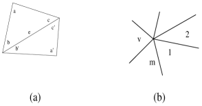
Figure 1.

The curvatures $\phi_{0}$ and $\psi_{0}$ were first introduced by I. Rivin [Ri] and G. Leibon [Le] respectively. If the surface $S=\mathbb{S}^{2}$, then these curvatures are essentially the dihedral angles of the associated 3-dimensional hyperbolic polyhedra at edges. The curvature $\phi_{-2}(e)=-\cot(a)-\cot(a^{\prime})$ is the discrete (cotangent) Laplacian operator on a polyhedral surface derived from the finite element approximation of the smooth Beltrami Laplacian on Riemannian manifolds.

One of the remarkable theorems proved by Rivin [15] is that a Euclidean polyhedral metric on a triangulated surface is determined up to scaling by its $\phi_{0}$ discrete curvature. In particular, he proved that an ideal convex hyperbolic polyhedron is determined up to isometry by its dihedral angles.

We prove,

Theorem 1.2.

Let $(S,T)$ be a closed triangulated connected surface. Then for any $h\in\mathbb{R}$,

(1) a Euclidean polyhedral metric on $(S,T)$ is determined up to isometry and scaling by its $\phi_{h}$ curvature.

(2) a spherical polyhedral metric on $(S,T)$ is determined up to isometry by its $\phi_{h}$ curvature.

(3) a hyperbolic polyhedral surface is determined up to isometry by its $\psi_{h}$ curvature.

We remark that theorem 1.2(1) for $h=0$ was aforementioned Rivin’s theorem. However, our proof of Rivin’s theorem is different from that in [15] and we use the variational principle established by Cohen-Kenyon-Propp [5]. Theorem 1.2(3) for $h=0$ was first proved by Leibon [11]. Theorem 1.2(2) for $h=0$ was proved in [14] and theorem 1.2(2) and (3) for $h\leq-1$ or $h\geq 0$ was proved in [12].

Take $h=-2$ in theorem 1.2, we obtain,

Corollary 1.3.

(1) A connected Euclidean polyhedral surface is determined up to scaling by its discrete Laplacian operator.

(2) A spherical polyhedral surface is determined by its discrete Laplacian operator.

Note that for a Euclidean polyhedral surface, $\phi_{h}=\psi_{h}$. There remain two questions on whether $\phi_{h}$ curvature determines a hyperbolic polyhedral surface or whether $\psi_{h}$ curvature determines a spherical polyhedral surface. It seems the results may still be true in these cases.

1.3.

Inversive distance circle packings are polyhedral metrics on a triangulated surface introduced by Bowers and Stephenson in [2]. An expansion of the discussion of [2] is in [3]. See also [16]. They are generalizations of Andreev and Thurston’s circle packings. Unlike the case of Andreev and Thurston where adjacent circles are intersecting, Bowers and Stephenson allow adjacent circles to be disjoint and measure their relative positions by the inversive distance. As observed in [2], this relaxation of intersection condition is very useful for practical applications of circle packing to many fields, including medical imaging and computer graphics. Based on extensive numerical evidences, they conjectured the rigidity and convergence of inversive distance circle packings in [2]. Our result shows that Bowers-Stephenson’s rigidity conjecture holds. The proof is based on a recent work of Ren Guo [9] which established a variational principle for inversive distance circle packings. A very nice geometric interpretation of the variational principle was given in [8].

We begin with a brief recall of the inversive distance in Euclidean, hyperbolic and spherical geometries. See [3] for a more detailed discussion. Let $K^{2}$ be $\mathbb{E}^{2}$, or $\mathbb{H}^{2}$ or $\mathbb{S}^{2}$. Given two circles $C_{1},C_{2}$ in $K^{2}$ centered at $v_{1},v_{2}$ of radii $r_{1}$ and $r_{2}$ so that $v_{1},v_{2}$ are of distance $l$ apart, the inversive distance $I=I(C_{1},C_{2})$ between the circles is given by

(1.3) $$I=\frac{l^{2}-r_{1}^{2}-r_{2}^{2}}{2r_{1}r_{2}}$$

in the Euclidean plane,

(1.4) $$I=\frac{\cosh(l)-\cosh(r_{1})\cosh(r_{2})}{\sinh(r_{1})\sinh(r_{2})}$$

in the hyperbolic plane and

(1.5) $$I=\frac{\cos(l)-\cos(r_{1})\cos(r_{2})}{\sin(r_{1})\sin(r_{2})}$$

in the 2-sphere. See [9] for more details on (1.4) and (1.5). If one considers $\mathbb{E}^{2}$, $\mathbb{H}^{2}$ and $\mathbb{S}^{2}$ as appeared in the infinity of the hyperbolic 3-space $\mathbb{H}^{3}$, then $C_{1}$ and $C_{2}$ are the boundary of two totally geodesic hyperplanes $D_{1}$ and $D_{2}$. The inversive distance $I$ is essentially the hyperbolic distance (or the intersection angle) between $D_{1}$ and $D_{2}$. In particular, for the Euclidean plane $\mathbb{E}^{2}$, the inversive distance $I(C_{1},C_{2})$ is invariant under the inversion and hence the name.

Bowers and Stephenson’s construction of an inversive distance circle packing with prescribed inversive distance on a triangulated surface $(S,T)$ is as follows. Fix once and for all a vector $I\in\mathbb{[}-1,\infty)^{E}$, called the inversive distance.

In the Euclidean case, for any $r\in\mathbb{R}_{>0}^{V}$, called the radius vector, define the edge length function $l\in\mathbb{R}_{>0}^{E}$ by the formula

(1.6) $$l(e)=\sqrt{r(v)^{2}+r(u)^{2}+2r(v)r(u)I(e)}$$

where the end points of the edge $e$ is $\{u,v\}$. If $l(e)$’s satisfy the triangular inequalities that

(1.7) $$l(e_{i})+l(e_{j})>l(e_{k})$$

for three edges $e_{i},e_{j},e_{k}$ of each triangle in $T$, then the length function $l:E\to\mathbb{R}$ sending $e$ to $l(e)$ defines a Euclidean polyhedral metric on $(S,T)$ called the inversive distance circle packing with inversive distance $I(e)$ at edge $e$. Note that if $I(e)\in[0,1]$ for all $e$, the polyhedral metric is the circle packing investigated by Andreev and Thurston where the intersection angle between two circles at the end points of an edge is $\arccos(I(e))$.

In the hyperbolic geometry, one uses

(1.8) $$l(e)=\cosh^{-1}(\cosh(r(v))\cosh(r(u))+I(e)\sinh(r(v))\sinh(r(u))$$

as the length of an edge. If (1.7) holds, then the lengths $l(e)$’s define a hyperbolic inversive distance circle packing with inversive distances $I$ on $(S,T)$. The spherical inversive distance circle packing is defined similarly with additional condition on $l(e)$’s that

$$l(e_{i})+l(e_{j})+l(e_{k})<2\pi$$

for each triangle with edges $e_{i},e_{j},e_{k}$.

The geometric meaning of these polyhedral metrics is the following. In each metric, if one draws a circle of radius $r(v)$ at each vertex $v$, then inversive distance of two circles at the end points of an edge $e$ is the given number $I(e)$.

Our result which solves Bowers-Stephenson’s rigidity conjecture is the following.

Theorem 1.4.

Given a closed triangulated connected surface $(S,T)$ with the set of edges $E$ and $I\in\mathbb{R}_{\geq 0}^{E}$ considered as the inversive distance,

(1) a hyperbolic inversive distance circle packing metric on $(S,T)$ of inversive distance $I$ is determined by its discrete curvature $k:V\to\mathbb{R}$.

(2) an Euclidean inversive distance circle packing metric on $(S,T)$ of inversive distance $I$ is determined by its discrete curvature $k:V\to\mathbb{R}$ up to scaling.

Note that for $I\in[0,1]^{E}$, the above result was Andreev-Thurston’s rigidity for circle packing with intersection angles between $[0,\pi/2]$. It seems the similar result may be true for $I\in[-1,\infty)^{E}$.

1.4.

The paper is organized as follows. In §2, we prove an extension lemma for angles of triangles. We also establish a criterion for extending a locally convex function to convex function. In §3, we prove theorem 1.4. Theorem 1.2 is proved in §4.

The following notations and conventions will be used in the paper. We use $\mathbb{R}$, $\mathbb{R}_{>0}$, $\mathbb{R}_{\geq 0}$, $\mathbb{R}_{<0}$ to denote the sets of all real numbers, positive real numbers, non-negative real numbers, and negative real numbers respectively. If $X$ is a set, $\mathbb{R}^{X}=\{f:X\to\mathbb{R}$} is the vector space of all functions on $X$. If $A$ is a subspace of a topological space $X$, then the closure of $A$ in $X$ is denoted by $\bar{A}$.

We thank Ren Guo for comments and careful reading of the manuscript.

2. Convex Extension of Locally Convex Functions

2.1. Continuous extension by constants

Definition 2.1.

Suppose $A$ is a subspace of a topological space $X$ and $f:A\to Y$ is continuous. If there exists a continuous function $F:X\to Y$ so that $F|_{A}=f$ and $F$ is a constant function on each connected component of $X-A$, then we say $f$ can be extended continuously by constant functions to $X$.

Note that if each connected component of $X-A$ intersects the closure of $A$, then the extension function $F$ is uniquely determined by $f$.

The key observation of the paper is the following simple lemma.

Lemma 2.2.

Suppose $\Delta$ is a triangle in the Euclidean plane $\mathbb{E}^{2}$, or the hyperbolic plane $\mathbb{H}^{2}$, or the 2-sphere $\mathbb{S}^{2}$ so that its edge lengths are $l_{1},l_{2},l_{3}$ and its inner angles are $\theta_{1},\theta_{2},\theta_{3}$. Assume that $\theta_{i}$’s angle is opposite to the edge of length $l_{i}$ for each $i$. Consider $\theta_{i}=\theta_{i}(l)$ as a function of $l=(l_{1},l_{2},l_{3})$.

1. If $\Delta$ is Euclidean or hyperbolic, the angle function $\theta_{i}$ defined on $\Omega=\{(l_{1},l_{2},l_{3})\in\mathbb{R}^{3}|l_{1}+l_{2}>l_{3},l_{2}+l_{3}>l_{1},l_{3}+l_{1}>l_{2}\}$ can be extended continuously by constant functions to a function $\tilde{\theta_{i}}$ on $\mathbb{R}^{3}_{>0}$.

2. If $\Delta$ is spherical, the angle function $\theta_{i}$ defined on $\Omega=\{(l_{1},l_{2},l_{3})\in\mathbb{R}^{3}|l_{1}+l_{2}>l_{3},l_{2}+l_{3}>l_{1},l_{3}+l_{1}>l_{2},l_{1}+l_{2}+l_{3}<2\pi\}$ can be extended continuously by constant functions to a function $\tilde{\theta_{i}}$ on $\mathbb{(}0,\pi)^{3}$.

We call the set $\Omega$ in the lemma the natural domain of the length vectors.

Proof.

In the case (1), the extension function $\tilde{\theta_{i}}$ of $\theta_{i}$ is given by $\tilde{\theta_{i}}=\pi$ when $l_{i}\geq l_{j}+l_{k}$, and $\tilde{\theta_{i}}=0$ when $l_{j}\geq l_{i}+l_{k}$. It remains to verify the continuity of $\tilde{\theta_{i}}$ on $\mathbb{R}_{>0}^{3}$. It is based on the cosine law. Given a point $L=(L_{1},L_{2},L_{3})$ in the boundary $\bar{\Omega}-\Omega$ of $\Omega$ inside $\mathbb{R}^{3}_{>0}$, we may assume without loss of generality that $L_{1}=L_{2}+L_{3}$. The continuity of $\tilde{\theta_{i}}$ follows from

$$\lim_{l\to L}\theta_{1}(l)=\pi,\quad\lim_{l\to L}\theta_{j}(l)=0,\quad j=2,3.$$

Indeed, the cosine law says, in the case of $\Delta\subset\mathbb{E}^{2}$, that

(2.1) $$\cos(\theta_{i})=\frac{l_{j}^{2}+l_{k}^{2}-l_{i}^{2}}{2l_{j}l_{k}}.$$

One sees easily that when $l$ tends to $L$, then the right-hand-side of (2.1) tends to $1$ if i=2,3 and $-1$ if $i=1$. This verifies the continuity in the Euclidean case. In the hyperbolic case, the cosine law says

(2.2) $$\cos(\theta_{i})=\frac{\cosh(l_{j})\cosh(l_{k})-\cosh(l_{i})}{\sinh(l_{j})\sinh(l_{k})}.$$

Thus one sees that as $l$ tends to $L=(L_{1},L_{2},L_{3})$ with $L_{j}>0$, the right-hand-side of (2.2) tends to $1$ if $i=2,3$ and to $-1$ if $i=1$. Thus $\tilde{\theta_{i}}$ is continuous.

To see (2), recall that the cosine law for spherical triangle says

(2.3) $$\cos(\theta_{i})=\frac{\cos(l_{i})-\cos(l_{j})\cos(l_{k})}{\sin(l_{j})\sin(l_{k})}.$$

If $l$ tends to $L$ where $L_{1}=L_{2}+L_{3}$ with $L_{i}\in(0,\pi)$, then $\lim_{l\to L}\cos(\theta_{1})=-1$ and $\lim_{l\to L}\cos(\theta_{i})=1$ when $i=2,3$. On the other hand, if $L_{1}+L_{2}+L_{3}=2\pi$ for $L_{i}\in(0,\pi)$, then the cosine law implies that $\lim_{l\to L}\cos(\theta_{i})=-1$ for all $i$, i.e., all inner angles are $\pi$ in this case. Thus by setting the extended function $\tilde{\theta_{i}}$ in $(0,\pi)^{3}$ to be $\tilde{\theta_{i}}(l)=\pi$ if $l_{i}\geq l_{j}+l_{k}$, $\tilde{\theta_{i}}(l)=0$ if $l_{j}\geq l_{i}+l_{k}$, and $\tilde{\theta_{i}}(l)=\pi$ if $l_{i}+l_{j}+l_{k}\geq\pi$, ( $\{i,j,k\}=\{1,2,3\}$), we see that $\tilde{\theta_{i}}$ is continuous.

∎

2.2. Continuous extension of 1-forms and of locally convex functions

We establish some simple facts on extending closed 1-forms and locally convex functions to convex functions in this subsection.

Definition 2.3.

A differential 1-form $w=\sum_{i=1}^{n}a_{i}(x)dx_{i}$ in an open set $U\subset\mathbb{R}^{n}$ is said to be continuous if each $a_{i}(x)$ is a continuous function on $U$. A continuous 1-form $w$ is called closed if $\int_{\partial\tau}w=0$ for each Euclidean triangle $\tau$ in $U$.

By the standard approximation theory, if $w$ is closed and $\gamma$ is a piecewise smooth null homologous loop in $U$, then $\int_{\gamma}w=0$. If $U$ is simply connected, then the integral $F(x)=\int_{a}^{x}w$ is well defined, independent of the choice of piecewise smooth paths in $U$ from $a$ to $x$. The function $F(x)$ is $C^{1}$-smooth so that $\partial F(x)/\partial x_{i}=a_{i}(x)$.

Proposition 2.4.

Suppose $X$ is an open set in $\mathbb{R}^{n}$ and $A\subset X$ is an open subset bounded by a smooth (n-1)-dimensional submanifold in $X$. If $w=\sum_{i=1}^{n}a_{i}(x)dx_{i}$ is a continuous 1-form on $X$ so that $w|_{A}$ and $w|_{X-\bar{A}}$ are closed where $\overline{A}$ is the closure of $A$ in $X$, then $w$ is closed in X.

Proof.

Since closedness is a local property and is invariant under smooth change of coordinates in $X$, we may assume that $X=\mathbb{R}^{n}$ and $A=\{(x_{1},...,x_{n})\in\mathbb{R}^{n}|x_{n}>0\}$. Take a Euclidean triangle $\tau\subset X$. To verify $\int_{\partial\tau}w=0$, we may assume that $\tau$ is not in $\overline{A}$ or $X-A$ since otherwise $\int_{\partial\tau}w=0$ follows from the assumption and the standard approximation theorem. In the remaining case, $\tau$ intersects both $A$ and $X-A$. The plane $x_{n}=0$ cuts the triangle $\tau$ into a triangle $\gamma_{1}$ and a quadrilateral $\gamma_{2}$ so that $\gamma_{1}$ and $\gamma_{2}$ are in the closure of $A$ and $X-A$. We can express, in the singular chain level, $\partial\tau=\partial\gamma_{1}+\partial\gamma_{2}$. By definition, $\int_{\partial\gamma_{i}}w=0$ for each $i$. Thus $\int_{\partial\tau}w=\int_{\partial\gamma_{1}}w+\int_{\partial\gamma_{2}}w=0$. ∎

A real analytic codimension-1 submanifold $Y$ in an open set $X$ in $\mathbb{R}^{n}$ is a smooth submanifold so that locally $Y$ is defined by $k(x)=0$ for a non-constant real analytic function $k$. Note that if $L$ is a (compact) line segment in $X$, then either $L\subset Y$ or $L\cap Y$ is a finite set. This is due to the fact that a non-constant real analytic function on an open interval has isolated zeros.

Recall that a function $f$ defined on a convex set $X\subset\mathbb{R}^{n}$ is called convex if for all $p,q\in X$ and all $t\in[0,1]$, $tf(p)+(1-t)f(q)\geq f(tp+(1-t)q)$. It is called strictly convex if for all $p\neq q$ in $X$ and all $t\in(0,1)$, $tf(p)+(1-t)f(q)>f(tp+(1-t)q)$. A function $f$ defined in an open set $U\subset\mathbb{R}^{n}$ is said to be locally convex (or locally strictly convex ) if it is convex (or strictly convex) in a convex neighborhood of each point.

Proposition 2.5.

Suppose $X\subset\mathbb{R}^{n}$ is an open convex set and $A\subset X$ is an open subset of $X$ bounded by a codimension-1 real analytic submanifold in $X$. If $w=\sum_{i=1}^{n}a_{i}(x)dx_{i}$ is a continuous closed 1-form on $X$ so that $F(x)=\int^{x}_{a}w$ is locally convex in $A$ and in $X-\overline{A}$, then $F(x)$ is convex in $X$.

Proof.

Since $X$ is simply connected, the function $F$ is well defined. To verify convexity, take $p,q\in X$ and consider $f(t)=F(tp+(1-t)q)$ for $t\in[0,1]$. It suffices to show that $f(t)$ is convex in $t$. Since $F$ is $C^{1}$-smooth, $f$ is $C^{1}$-smooth. Let $\partial A=\bar{A}-A$ and $L$ be the line segment from $p$ to $q$. Since $\partial A$ is real analytic, either $L$ intersects $\partial A$ in a finite set of points, or $L$ is in $\partial A$. In the first case, let $0=t_{0}<t_{1}<...,t_{n}=1$ be the partition of $[0,1]$ so that the line segment $tp+(1-t)q$ for $t\in(t_{i},t_{i+1})$ is either in $A$ or in $X-\overline{A}$. By definition, $f(t)$ is convex in $[t_{i},t_{i+1}]$, i.e., $f^{\prime}(t)$ is increasing in $[t_{i},t_{i+1}]$ for $i=0,...,n-1$. Since $f^{\prime}(t)$ is continuous in $[0,1]$, this implies that $f^{\prime}(t)$ is increasing in $[0,1]$, i.e., $f(t)$ is convex in $[0,1]$. In the second case that $L\subset\partial A$, we take two sequences of points $p_{m}$ and $q_{m}$ converging to $p$ and $q$ respectively in $X$ so that $p_{m},q_{m}$ are not in $\partial A$. Then by the case just proved, the functions $f_{m}(t)=F(tp_{m}+(1-t)q_{m})$ are convex in $t$. Furthermore, $f_{m}$ converges to $f$. Thus $f$ is convex. ∎

Corollary 2.6.

Suppose $X\subset\mathbb{R}^{n}$ is an open convex set and $A\subset X$ is an open subset of $X$ bounded by a real analytic codimension-1 submanifold in $X$. If $w=\sum_{i=1}^{n}a_{i}(x)dx_{i}$ is a continuous closed 1-form on $A$ so that $F(x)=\int^{x}_{a}w$ is locally convex on $A$ and each $a_{i}$ can be extended continuously to $X$ by constant functions to a function $\tilde{a_{i}}$ on $X$, then $\tilde{F}(x)=\int^{x}_{a}\sum_{i=1}^{n}\tilde{a_{i}}dx_{i}$ is a $C^{1}$-smooth convex function on $X$ extending $F$.

We remark that the real analytic assumption in the proposition 2.5 can be relaxed to $C^{2}$ smooth.

3. A Proof of Bowers-Stephenson’s Rigidity Conjecture

We begin by recalling Guo’s work on a variational principle associated to inversive distance circle packings and then prove theorem 1.4. We will work in Euclidean and hyperbolic geometries only.

3.1. Guo’s variational principle for inversive distance circle packing

Suppose $\Delta$ is a triangle with vertices $v_{1},v_{2},v_{3}$ and edges $e_{ij}=v_{i}v_{j}$, $i\neq j$. Fix once and for all an inversive distance $I_{ij}\in[0,\infty)$ at each edge $e_{ij}$. Then for each assignment of positive number $r_{i}$ at $v_{i}$ for $i=1,2,3$, let

(3.1) $$l_{k}=\sqrt{r_{i}^{2}+r_{j}^{2}+2r_{i}r_{j}I_{ij}}$$

for Euclidean geometry and

(3.2) $$l_{k}=\cosh^{-1}(\cosh(r_{i})\cosh(r_{j})+I_{ij}\sinh(r_{i})\sinh(r_{j}))$$

for hyperbolic geometry where $\{i,j,k\}=\{1,2,3\}$.

Let $\Omega=\{(x_{1},x_{2},x_{3})\in\mathbb{R}_{>0}^{3}|x_{i}+x_{j}>x_{k},\{i,j,k\}=\{1,2,3\}\}$. If $(l_{1},l_{2},l_{3})$ is in $\Omega$, then we construct a Euclidean triangle $\Delta$ with length $l_{k}$ of $e_{ij}$ given by (3.1) and a hyperbolic triangle, still denoted by $\Delta$, with length $l_{k}$ of $e_{ij}$ given by (3.2). Suppose the angle of the triangle at $v_{i}$ is $\theta_{i}$ and consider $\theta_{i}$ as a function of $(r_{1},r_{2},r_{3})$. Guo proved the following theorem in [9].

Theorem 3.1.

(Guo [9]) Fix any $(I_{12},I_{23},I_{31})\in[0,\infty)^{3}$.

(1) For Euclidean triangles, let $u_{i}=\ln r_{i}$, then the differential 1-form $w=\sum_{i=1}^{3}\theta_{i}du_{i}$ is closed in the open subset of $\mathbb{R}^{3}$ where it is defined. The integral $F(u)=\int_{0}^{u}w$ is a locally concave function in $u=(u_{1},u_{2},u_{3})$ and is strictly locally concave in $u_{1}+u_{2}+u_{3}=0$. Furthermore, if $c\in\mathbb{R}$ and $F(u)$ is defined, then $F(u+(c,c,c))=F(u)$.

(2) For hyperbolic triangles, let $u_{i}=\ln(\tanh(r_{i}/2))$, then the differential 1-form $w=\sum_{i=1}^{3}\theta_{i}du_{i}$ is closed in the open subset of $\mathbb{R}_{<0}^{3}$ where it is defined. Furthermore, the integral $F(u)=\int_{-(1,1,1)}^{u}w$ is a strictly locally concave function in $u=(u_{1},u_{2},u_{3})$.

It is also proved in [9] that the open sets where the 1-forms $w$ are defined in theorem 3.1 are connected and simply connected. Theorem 3.1 is a generalization of an earlier result obtained in [6]. Guo proved a local and infinitesimal rigidity theorem for inversive distance circle packing using theorem 3.1. It says that a Euclidean inversive distance circle packing is locally determined, up to scaling, by the discrete curvature of the underlying polyhedral surface. He also proved the local and infinitesimal rigidity for hyperbolic inversive distance circle packings.

3.2. Concave extension of Guo’s action functional

Our main observation is that Guo’s differential 1-forms $w=\sum_{i=1}^{3}\theta_{i}du_{i}$ can be extended to a closed 1-form on $\mathbb{R}^{3}$ in the Euclidean case and on $\mathbb{R}^{3}_{<0}$ in the hyperbolic case so that the integrations of the extended 1-forms are still concave.

Proposition 3.2.

Let $w$ be the 1-forms defined in theorem 3.1.

(a) In the case of Euclidean triangles, the 1-form $w$ can be extended to a continuous closed 1-form $\tilde{w}$ on $\mathbb{R}^{3}$ so that the integration $\tilde{F}(u)=\int^{u}_{0}\tilde{w}$ is a $C^{1}$-smooth concave function.

(b) In the case of hyperbolic triangles, the 1-form $w$ can be extended to a continuous closed 1-form $\tilde{w}$ on $\mathbb{R}_{<0}^{3}$ so that the integration $\tilde{F}(u)=\int^{u}_{-(1,1,1)}\tilde{w}$ is a $C^{1}$-smooth concave function.

We begin by focusing the 1-forms in its radius coordinate $r=(r_{1},r_{2},r_{3})\in\mathbb{R}_{>0}^{3}$. In this case, the 1-forms are given by $w=\sum_{i=1}^{3}\theta_{i}\frac{dr_{i}}{r_{i}}$ and $w=\sum_{i=1}^{3}\theta_{i}\frac{dr_{i}}{\sinh(r_{i})}$. The 1-form $w$ is defined on the open set $U$ of $\mathbb{R}_{>0}^{3}$ where

(3.3) $$U=\{(r_{1},r_{2},r_{3})\in\mathbb{R}_{>0}^{3}|l_{i}+l_{j}>l_{k},\{i,j,k\}=\{1,2,3\}\},$$

where $l_{i}=l_{i}(r_{1},r_{2},r_{3})$ is defined on $\mathbb{R}_{>0}^{3}$. (Note that for hyperbolic and Euclidean geometries, the sets $U$ are different due to (3.1) and (3.2)). The extension of the 1-form $w$ is the natural one. Namely, we replace $\theta_{i}$ in $w$ by $\tilde{\theta_{i}}$ appeared in lemma 2.1. Thus the extended 1-form is $\tilde{w}=\sum_{i=1}^{3}\tilde{\theta_{i}}\frac{dr_{i}}{r_{i}}$ or $\tilde{w}=\sum_{i=1}^{3}\tilde{\theta_{i}}\frac{dr_{i}}{\sinh(r_{i})}.$

It remains to show that $\tilde{w}$ is continuous and closed in $\mathbb{R}_{>0}^{3}$ so that its pull back to the $u$-coordinate has a concave integration. To this end, we prove,

Lemma 3.3.

Let $\bar{U}$ be the closure of $U$ in $\mathbb{R}_{>0}^{3}$. Then,

(1) $\theta_{i}$ is a constant function on each connected component of $\bar{U}-U$, and

(2) for each connected component $V$ of $\mathbb{R}_{>0}^{3}-U$, the intersection $V\cap\bar{U}$ is a connected component of $\bar{U}-U$.

Proof.

By (3.3), the boundary $\partial U=\bar{U}-U$ is given by $\cup_{i=1}^{3}\partial_{i}U$ where $\partial_{i}U=\{(r_{1},r_{2},r_{3})\in\mathbb{R}_{>0}^{3}|l_{i}=l_{j}+l_{k},\{j,k\}=\{1,2,3\}-\{i\}\}$. Furthermore, $\mathbb{R}_{>0}^{3}-U=\cup_{i=1}^{3}V_{i}$ where $V_{i}=\{(r_{1},r_{2},r_{3})\in\mathbb{R}_{>0}^{3}|l_{i}\geq l_{j}+l_{k},\{j,k\}=\{1,2,3\}-\{i\}\}.$

First, we note that if $I_{ij}\leq 1$, then $\partial_{k}U=\emptyset$ and $V_{k}=\emptyset$. Indeed, if $I_{ij}\leq 1$, then by (3.1) and (3.2),

$$l_{k}\leq r_{i}+r_{j}.$$

But due to $I_{ab}\geq 0$, (3.1) and (3.2), $r_{j}<l_{i}$ and $r_{i}<l_{j}$. Therefore, $l_{k}<l_{i}+l_{j}$. This implies that $\partial_{k}U=\emptyset$ and $V_{k}=\emptyset$.

Next $\partial_{i}U\cap\partial_{j}U=\emptyset$ and $V_{i}\cap V_{j}=\emptyset$ for $i\neq j$. Indeed, if $r\in\partial_{i}U\cap\partial_{j}U$ or $r\in V_{i}\cap V_{j}$, then $l_{i}\geq l_{j}+l_{k}$ and $l_{j}\geq l_{i}+l_{k}$. Thus $l_{k}=0$. But $l_{k}>r_{i}>0$.

We claim that if $I_{ij}>1$, then both $V_{k}$ and $\partial_{k}U$ are non-empty and connected. Assume the claim, then the lemma follows. Indeed, since $l_{s}>0$ for all indices $s$, it follows, by lemma 2.1, that $\theta_{i}$ is either $0$ or $\pi$ in $\partial_{s}U$, i.e., (1) holds. Next, $V_{s}$’s are the connected components of $\mathbb{R}_{>0}^{3}-U$ so that $V_{s}\cap\bar{U}=\partial_{s}U$. Thus (2) holds.

To see the claim, it suffices to show that there is a smooth function $f(r_{i},r_{j})$ defined on $\mathbb{R}_{>0}^{3}$ so that its graph is $\partial_{k}U$ and $V_{k}=\{(r_{1},r_{2},r_{3})\in\mathbb{R}_{>0}^{3}|0<r_{3}\leq f(r_{1},r_{2})\}$.

To this end, consider the equation

(3.4) $$l_{k}=l_{i}+l_{j},$$

and let the right-hand-side of (3.4) be $g(r_{k},r_{i},r_{j})$. We will deal with the Euclidean and hyperbolic geometry separately.

CASE 1 Euclidean triangles. In this case, the function $g(r_{k},r_{i},r_{j})$ is given by

(3.5) $$g(r_{k},r_{i},r_{j})=\sqrt{r_{k}^{2}+r_{j}^{2}+2I_{kj}r_{k}r_{j}}+\sqrt{r_{i}^{2}+r_{k}^{2}+2I_{ik}r_{i}r_{k}}$$

Evidently, for a fixed $(r_{i},r_{j})\in\mathbb{R}^{2}_{>0}$, $g(r_{k},r_{i},r_{j})$ is a strictly increasing function of $r_{k}\in\mathbb{R}_{>0}$ so that $g(0,r_{i},r_{j})=r_{i}+r_{j}<\sqrt{r_{i}^{2}+r_{j}^{2}+2I_{ij}r_{i}r_{j}}$ (due to $I_{ij}>1$) and $\lim_{r_{k}\to\infty}g(r_{k},r_{i},r_{k})=\infty$. By the mean-value theorem, there exists a unique positive number $f(r_{i},r_{j})$ so that $g(f(r_{i},r_{j}),r_{i},r_{j})=\sqrt{r_{i}^{2}+r_{j}^{2}+2r_{i}r_{j}I_{ij}}=l_{k}$. The smoothness of $f(r_{i},r_{j})$ follows from the implicit function theorem applied to (3.4). Indeed,

$$\frac{\partial g}{\partial r_{k}}=\frac{r_{k}+2I_{kj}r_{j}}{l_{i}}+\frac{r_{k}+2I_{ik}r_{i}}{l_{j}}>0.$$

Thus, $f(r_{i},r_{j})$ is smooth.

This shows $\partial_{k}U$ is the graph of the smooth function $f$ defined on $\mathbb{R}_{>0}^{2}$, i.e.,

$$\partial_{k}U=\{(r_{1},r_{2},r_{3})\in\mathbb{R}_{>0}^{3}|r_{k}=f(r_{i},r_{j})\}.$$

Thus it is connected. Since $g(r_{k},r_{i},r_{j})$ is an increasing function of $r_{k}$, $V_{k}=\{r\in R_{>0}^{3}|0<r_{k}\leq f(r_{i},r_{j}),\{i,j\}=\{1,2,3\}-\{k\}\}$. Thus $V_{k}$ is connected.

CASE 2 hyperbolic triangles. By the same argument as in case 1, it suffices to show the same properties established in case 1 hold for $g(r_{k},r_{i},r_{j})$ given by

(3.6) $$\cosh^{-1}(\cosh(r_{i})\cosh(r_{k})+I_{ik}\sinh(r_{i})\sinh(r_{k}))+\cosh^{-1}(\cosh(r_{k})\cosh(r_{j})+I_{kj}\sinh(r_{k})\sinh(r_{j})).$$

Fix $(r_{i},r_{j})\in\mathbb{R}^{2}_{>0}$. Then the function $g(r_{k},r_{i},r_{j})$ is clearly strictly increasing in $r_{k}\in\mathbb{R}_{>0}$ so that $\lim_{r_{k}\to\infty}g(r_{k},r_{i},r_{j})=\infty$ and due to $I_{ij}>1$,

$$g(0,r_{i},r_{j})=r_{i}+r_{j}$$

$$=\cosh^{-1}(\cosh(r_{i}+r_{j}))$$

$$=\cosh^{-1}(\cosh(r_{i})\cosh(r_{j})+\sinh(r_{i})\sinh(r_{j}))$$

$$<\cosh^{-1}(\cosh(r_{i})\cosh(r_{j})+I_{ij}\sinh(r_{i})\sinh(r_{j}))=l_{k}.$$

By the mean value theorem, there exists a unique positive number $f(r_{i},r_{j})$ so that $g(f(r_{i},r_{j}),r_{i},r_{j})=l_{k}$. The smoothness of $f(r_{i},r_{j})$ follows form the implicit function theorem that

$$\frac{\partial g}{\partial r_{k}}=\frac{\cosh(r_{i})\sinh(r_{k})+I_{ik}\sinh(r_{i})\cosh(r_{k})}{\sqrt{(\cosh(r_{i})\cosh(r_{k})+I_{ik}\sinh(r_{i})\sinh(r_{k}))^{2}-1}}$$

$$+\frac{\cosh(r_{j})\sinh(r_{k})+I_{jk}\sinh(r_{j})\cosh(r_{k})}{\sqrt{(\cosh(r_{j})\cosh(r_{k})+I_{jk}\sinh(r_{j})\sinh(r_{k}))^{2}-1}}$$

$$>0.$$

By the same argument as in case 1, we see that $\partial_{k}U$, being the graph of the smooth function $f$, is connected and $V_{k}$, being the region below the positive function $f$ over $\mathbb{R}^{2}_{>0}$, is also connected. ∎

Now back to the proof of proposition 3.2, for part (1), consider the real analytic diffeomorphism $u=u(r):\mathbb{R}^{3}_{>0}\to\mathbb{R}^{3}$ where $u_{i}=\ln r_{i}$. The differential 1-form $w=\sum_{i=1}^{3}\theta_{i}\frac{dr_{i}}{r_{i}}$ pulls back (via $r=u^{-1}(r)$) to $w=\sum_{i=1}^{3}\theta_{i}du_{i}$ as appeared in theorem 3.1. By lemma 3.3, the extension $\tilde{w}=\sum_{i=1}^{3}\tilde{\theta_{i}}du_{i}$ is obtained from $w$ by extending each coefficient $\theta_{i}$ by constant functions on $\mathbb{R}^{3}-u^{-1}(U)$. Thus, by corollary 2.6, the function $\tilde{F}(u)=\int^{u}_{0}\tilde{w}$ is a $C^{1}$-smooth concave function in $u\in\mathbb{R}^{3}$ so that

(3.7) $$\partial\tilde{F}/\partial u_{i}=\tilde{\theta_{i}}.$$

The same argument also works for part (2) since $u=u(r)$ with $u_{i}=\ln\tanh(r_{i})$ is a real analytic diffeomorphism from $\mathbb{R}_{>0}^{3}$ onto $\mathbb{R}_{<0}^{3}$.

3.3. A proof of theorem 1.4 for Euclidean inversive distance circle packing

Suppose otherwise that there exist two inversive circle packing metrics $d_{1},d_{2}$ on $(S,T)$ with the same inversive distance $I\in\mathbb{[}0,\infty)^{E}$ so that their discrete curvatures are the same and $d_{1}\neq\lambda d_{2}$ for any $\lambda$. Let $a\in\mathbb{R}^{V}$ be their common discrete curvature.

We will use the notation that if $i\in V$ and $x\in\mathbb{R}^{V}$, then $x_{i}=x(i)$ below. Let $T^{(2)}$ be the set of all triangles in $T$. If a triangle $s\in T^{(2)}$ has vertices $i,j,k\in V$, then we denote the triangle by $s=\{i,j,k\}$. For circle packing metrics of radii $r\in\mathbb{R}_{>0}^{V}$ with a given inversive distance $I$, we use $u\in\mathbb{R}^{V}$ to denote their logarithm coordinate where $u_{i}=\ln r_{i}$. Thus, there are two points $p,q$ in $\mathbb{R}^{V}$ as the logarithmic coordinates of $d_{1}$ and $d_{2}$ so that their discrete curvatures are $a\in\mathbb{R}^{V}$ and $p-q\neq\lambda(1,1,1,..,1)$ for any $\lambda$.

We will derive a contradiction by using the locally concave functions $F$ and its concave extension $\tilde{F}=\int^{u}_{0}\tilde{w}$ appeared in proposition 3.2 associated to theorem 3.1(1).

Define a $C^{1}$-smooth function $W:\mathbb{R}^{V}\to\mathbb{R}$ by

(3.8) $$W(u)=-\sum_{s\in T^{(2)},s=\{i,j,k\},i,j,k\in V}\tilde{F}(u_{i},u_{j},u_{k})+\sum_{i\in V}(2\pi-a_{i})u_{i}.$$

The function $W$ is convex since it is a summation of convex functions. Furthermore, by the definition of $W$, (3.7), the definition of discrete curvature $(a_{i})$, $p$ and $q$ are both critical points of $W$. Since $W$ is convex in $\mathbb{R}^{V}$, $p$ and $q$ are both minimal points of $W$. Furthermore, for all $t\in[0,1]$, $tp+(1-t)q$ are minimal points of $W$. In particular,

$$W(tp+(1-t)q)=W(p)$$

for all $t\in[0,1]$. Since

$$W(tp+(1-t)q)=\sum_{s\in T^{(2)},s=\{i,j,k\},i,j,k\in V}f_{ijk}(t)+\sum_{i\in E}(2\pi-a_{i})(tp_{i}+(1-t)q_{i})$$

where the function

(3.9) $$f_{ijk}(t)=-\tilde{F}(tp_{i}+(1-t)q_{i},tp_{j}+(1-t)q_{j},tp_{k}+(1-t)q_{k})$$

is convex, it follows that $f_{ijk}(t)$ is linear in $t\in[0,1]$ for all triangle $s$ with vertices $i,j,k$. This is due to the simple fact that a summation of a convex function with a strictly convex function is strictly convex. By the assumption that $p-q\neq c(1,1,....,1)$ in $\mathbb{R}^{V}$ and the surface is connected, there exists a triangle $s$ with vertices $i,j,k\in V$ so that $(p_{i},p_{j},p_{k})-(q_{i},q_{j},q_{k})\neq(c,c,c)$ for all $c\in\mathbb{R}$. By the given assumption, $(p_{i},p_{j},p_{k})$ and $(q_{i},q_{j},q_{k})$ are in the domain of definition of $w$ in theorem 3.1. Thus for $t\in[0,1]$ close to $0$ or $1$, by theorem 3.1 on the local strictly convexity of $-F(u_{1},u_{2},u_{3})$ on $u_{1}+u_{2}+u_{3}=0$ and $F(u+(c,c,c))=F(u)$, $f_{ijk}(t)$ is strictly convex in $t$ near $0,1$. This is a contradiction to the linearity of $f_{ijk}(t)$.

3.4. A proof of theorem 1.4 for hyperbolic inversive distance circle packing

The proof is essentially the same as in §3.3 and is simpler. For any $r\in\mathbb{R}_{>0}^{V}$, define $u=u(r)\in\mathbb{R}_{<0}^{V}$ by $u_{i}=\ln\tanh(r_{i}/2))$. For a circle packing with radii $r\in\mathbb{R}_{>0}^{V}$, let $u=u(r)$ and call it the $u$-coordinate of the circle packing metric.

We use the same notation as in §3.3. Suppose the result does not hold and let $p\neq q\in\mathbb{R}_{<0}^{V}$ be the $u$-coordinates of the two distinct hyperbolic circle packing metrics having the same hyperbolic inversive distance $I\in\mathbb{R}_{\geq 0}^{E}$ and the same discrete curvature $a=(a_{i})\in\mathbb{R}^{V}$. Define the action functional $W$ on $\mathbb{R}_{<0}^{V}$ by the same formula (3.8) where $\tilde{F}$ is the concave function in proposition 3.2 associated to theorem 3.1(2). Then the same proof goes through as in §3.3 since in this case, one of $f_{ijk}(t)$ is strictly convex for $t$ near 0 and 1.

4. 2-dimensional Schlaefli Type Action Functionals and Their Extensions

The following was proved in [12]. The proof is a straight forward calculation.

Theorem 4.1.

Suppose $\Delta$ is a triangle in the Euclidean plane $\mathbb{E}^{2}$, or the hyperbolic plane $\mathbb{H}^{2}$, or the 2-sphere $\mathbb{S}^{2}$ so that its edge lengths are $l_{1},l_{2},l_{3}$ and its inner angles are $\theta_{1},\theta_{2},\theta_{3}$ where $\theta_{i}$’s angle is opposite to the edge of length $l_{i}$. Let $h\in\mathbb{R}$ and let $\Omega$ be the natural domain for length vectors appeared in lemma 2.2.

1. For a Euclidean triangle,

   $$w_{h}=\sum_{i=1}^{3}\frac{\int^{\theta_{i}}_{\pi/2}\sin^{h}(t)dt}{l_{i}^{h+1}}dl_{i}$$

   is a closed 1-form on $\Omega$. The integral $\int^{u}_{-(h,h,h)}w_{h}$ is locally convex in variable $u=(u_{1},u_{2},u_{3})$ where $u_{i}=\ln l_{i}$ for $h=0$ and $u_{i}=-\frac{l_{i}^{-h}}{h}$ for $h\neq 0$. Furthermore, $\int^{u}_{-(h,h,h)}w_{h}$ is locally strictly convex in hypersurface $u_{1}+u_{2}+u_{3}=0$.

2. For a spherical triangle,

   $$w_{h}=\sum_{i=1}^{3}\frac{\int^{\theta_{i}}_{\pi/2}\sin^{h}(t)dt}{\sin^{h+1}(l_{i})}dl_{i}$$

   is a closed 1-form on $\Omega$. The integral $\int^{u}_{0}w_{h}$ is locally strictly convex in $u=(u_{1},u_{2},u_{3})$ where $u_{i}=\int^{l_{i}}_{\pi/2}$ $\sin^{-h-1}(t)dt$.

3. For a hyperbolic triangle,

   $$w_{h}=\sum_{i=1}^{3}\frac{\int^{\theta_{i}}_{\pi/2}\sin^{h}(t)dt}{\sinh^{h+1}(l_{i})}dl_{i}$$

   is a closed 1-form.

4. For a hyperbolic triangle,

   $$w_{h}=\sum_{i=1}^{3}\frac{\int^{\frac{1}{2}(\theta_{i}-\theta_{j}-\theta_{k})}_{0}\cos^{h}(t)dt}{\coth^{h+1}(l_{i}/2)}dl_{i}$$

   is a closed 1-form. The integral $\int^{u}_{0}w_{h}$ is locally strictly convex in $u=(u_{1},u_{2},u_{3})$ where $u_{i}=\int^{l_{i}}_{1}$ $\coth^{-h-1}(t/2)dt$.

4.1.

Recall that the natural domain $\Omega$ of the edge length vectors is given by $\Omega=\{(l_{1},l_{2},l_{3})\in\mathbb{R}_{>0}^{3}|l_{i}+l_{j}>l_{k},\{i,j,k\}=\{1,2,3\}\}$ for Euclidean and hyperbolic triangles and $\Omega=\{(l_{1},l_{2},l_{3})\in\mathbb{R}_{>0}^{3}|l_{i}+l_{j}>l_{k},l_{1}+l_{2}+l_{3}<2\pi,\{i,j,k\}=\{1,2,3\}\}$. Let $J$ be the natural interval for each individual length $l_{i}$, i.e., $J=\mathbb{R}_{>0}$ for Euclidean and hyperbolic triangles and $J=(0,\pi)$ for spherical triangles. In each case of theorem 4.1, there exists a real analytic diffeomorphism $g:J\to g(J)$ from $J$ onto the open interval $g(J)$ so that $u_{i}=g(l_{i})$. To be more precise, $g(t)=\ln t$ in the case of $h=0$ of theorem 4.1(1), $g(t)=-\frac{t^{-h}}{h}$ ($h\neq 0$) in the case of $h\neq 0$ in theorem 4.1(1), $g(t)=\int^{t}_{\pi/2}\sin^{-h-1}(x)dx$ in the case (2) of theorem 4.1, $g(t)=\int^{t}_{1}\sinh^{-h-1}(x)dx$ in the case (3) of theorem 4.1 and $g(t)=\int^{t}_{1}\coth^{-h-1}(x)dx$ in the case of (4). The real analytic diffeomorphism $u(l_{1},l_{2},l_{3})=(u_{1},u_{2},u_{3})$ where $u_{i}=g(l_{i})$ sends $J^{3}$ onto the open cube $g(J)^{3}$ in $\mathbb{R}^{3}$.

By lemma 2.2, each of the angle function $\theta_{i}(l):\Omega\to\mathbb{R}$ can be extended by constant functions to a continuous function $\tilde{\theta_{i}}(l):J^{3}\to\mathbb{R}$. Define a continuous 1-form $\tilde{w_{h}}$ on $J^{3}$ by replacing $\theta_{i}$ in the definition of $w_{h}$ in theorem 4.1 by $\tilde{\theta_{i}}$.

Lemma 4.2.

The continuous differential 1-form $\tilde{w_{h}}$ is closed in $J^{3}$.

Proof.

By proposition 2.4 where we take $X=J^{3}$ and $A=\Omega$, it suffices to show that $\tilde{w_{h}}$ is closed in each connected component $U$ of $J^{3}-\overline{\Omega}$. By theorem 4.1 $\tilde{w}|_{A}$ is closed, the restriction of $\tilde{w_{h}}$ to $U$ is of the form $\sum_{i=1}^{3}c_{i}du_{i}$ where $u_{i}=g(l_{i})$ and $c_{i}$ is a constant. Thus $\tilde{w_{h}}|_{U}$ is closed. ∎

Proposition 4.3.

The pull back 1-form $(u^{-1})^{*}(\tilde{w_{h}})$ on $g(J)^{3}$ is a closed 1-form. Furthermore, if $F(u)=\int^{u}w_{h}$ is locally convex in $u(\Omega)$ (i.e, in the case (1),(2), (4) of theorem 4.1), then $\tilde{F}(u)=\int^{u}(u^{-1})^{*}(\tilde{w_{h}})$ is convex in $u$ in $g(J)^{3}$.

Note that by the construction, if $u\in u(\Omega)$ and $w_{h}=\sum_{i=1}^{3}\alpha_{i,h}(u)du_{i}$ (as shown in theorem 4.1) then

(4.1) $$\frac{\partial\tilde{F}(u)}{\partial u_{i}}=\alpha_{i,h}(u).$$

Furthermore, by definition, the $\phi_{h}$ and $\psi_{h}$ curvatures are sum of two of $a_{i,h}(u)$’s.

Proof.

By corollary 2.6 where we take $X=g(J)^{3}$ and $A=u(\Omega)$, it suffices to show that $u(\Omega)$ is bounded by a real analytic surface in $X$ and $\tilde{F}(u)$ is convex in $u(\Omega)$ and in each component of $g(J)^{3}-\overline{u(\Omega)}$.

Since $\Omega$ in $J^{3}$ is bounded by hyperplanes and $u(l)=(g(l_{1}),g(l_{2}),g(l_{3}))$ is a real analytic diffeomorphism, it follows that $u(\Omega)$ is bounded by a real analytic surface in $g(J)^{3}$.

By the assumption $\tilde{F}(u)$ is convex in $u(\Omega)$. If $U$ is a connected component of $g(J)^{3}-\overline{u(\Omega)}$, then $\tilde{F}(u)$ is linear on $U$ since its partial derivatives are constants on $U$ by the construction. Thus by corollary 2.6, the result follows. ∎

5. A Proof of Theorem 1.2

The argument is essentially the same as that in §3.3. Recall that $E$ is the set of all edges in the triangulated surface $(S,T)$. If $x\in\mathbb{R}^{E}$ and $i\in E$, we use $x_{i}$ to denote $x(i)$. If $s\in T^{(2)}$ is a triangle with edges $i,j,k\in E$, we denote it by $s=\{i,j,k\}$.

5.1. A proof of theorem 1.2(3)

Suppose otherwise that there exist two distinct hyperbolic polyhedral metrics on $(S,T)$ so that their $\psi_{h}$ curvatures are the same. Let $a=(a_{i})\in\mathbb{R}^{E}$ be their common $\psi_{h}$ curvature.

Recall that a polyhedral metric on $(S,T)$ is given by its edge length map $l:E\to\mathbb{R}_{>0}$. In using the variational principle in theorem 4.1(4), the natural variable is given by $u:E\to\mathbb{R}$ where $u(e)=g(l(e))$ with $g(t)=\int^{t}_{1}\coth^{h+1}(s/2)ds$. We call it the $u$-coordinate of the polyhedral metric $l$ and we will use the $u$-coordinate to set up the variational principle. Therefore there are two distinct points (as $u$-coordinates) $p\neq q\in g(\mathbb{R}_{>0})^{E}$ so that their corresponding $\psi_{h}$ curvatures are the same $a\in\mathbb{R}^{E}$. We will derive a contradiction by using the locally strictly convex functions $F$ and its convex extension $\tilde{F}$ introduced in proposition 4.3 (associated to theorem 4.1(4)).

Define a $C^{1}$-smooth function $W:g(\mathbb{R}_{>0})^{E}\to\mathbb{R}$ by

$$W(u)=\sum_{s\in T^{(2)},s=\{i,j,k\},i,j,k\in E}\tilde{F}(u_{i},u_{j},u_{k})-\sum_{i\in E}a_{i}u_{i}.$$

The function $W$ is convex since it is a summation of convex functions. Furthermore, by the definition of $W$, (4.1), the definition of $\psi_{h}$ and $(a_{i})$, $p$ and $q$ are both critical points of $W$. Since $W$ is convex, $p$ and $q$ are both minimal points of $W$. Furthermore, for all $t\in[0,1]$, $tp+(1-t)q$ are minimal points of $W$. In particular,

$$W(tp+(1-t)q)=W(p)$$

for all $t\in[0,1]$. Since

$$W(tp+(1-t)q)=\sum_{i,j,k\in E,\{i,j,k\}\in T^{(2)}}f_{ijk}(t)-\sum_{i\in E}a_{i}(tp_{i}+(1-t)q_{i})$$

where the function

(5.1) $$f_{ijk}(t)=\tilde{F}(tp_{i}+(1-t)q_{i},tp_{j}+(1-t)q_{j},tp_{k}+(1-t)q_{k})$$

is convex, it follows that $f_{ijk}(t)$ is linear in $t\in[0,1]$. Since $p\neq q$, there exists a triangle with edges $i,j,k\in E$ so that $(p_{i},p_{j},p_{k})\neq(q_{i},q_{j},q_{k})$. Thus for $t\in[0,1]$ close to $0$ or $1$, by theorem 4.1 on the local strictly convexity, $f_{ijk}(t)$ is strictly convex in $t$ near $0,1$. This is a contradiction to the linearity of $f_{ijk}(t)$.

5.2. A proof of theorem 1.2(2)

The proof is exactly the same as above using the extended convex function $\tilde{F}$ in proposition 4.3 associated to theorem 4.1(2).

5.3. A proof of theorem 1.2(1)

The proof is the same as that in §5.1 using the similarly defined function $W$. To be more precise, let $g(t)=-\frac{t^{-h}}{h}$ for $h\neq 0$ and $g(t)=\ln t$. By the same set up as in §5.1, we conclude that $f_{ijk}(t)$ given by (5.1) is linear in $t$. We claim this implies that the two Euclidean polyhedral metrics $u^{-1}(p)$ and $u^{-1}(q)$ differ by a scalar multiplication. There are two cases to be discussed depending on $h=$ or $h\neq 0$.

CASE 1. $h=0$. In this case, $p-q\neq c(1,1,...,1)$ in $\mathbb{R}^{E}$ for any constant $c$. By the connectivity of the surface $S$, there exists a triangle with edges $i,j,k\in E$ so that $(p_{i},p_{j},p_{k})-(q_{i},q_{j},q_{k})\neq(c,c,c)$ for any constant $c$. On the other hand, by theorem 4.1(1), the action functional $F$ is strictly locally convex in the hyperplane $u_{1}+u_{2}+u_{3}=0$ and $F(u+(c,c,c)=F(u)$ for a scalar $c$ and $u\in u(\Omega)$. In particular, this implies that the function $f_{ijk}(t)$ is strictly convex in $t\in[0,1]$ for $t$ close to $0$ or $1$. This contradicts the linearity of the function $f_{ijk}(t)$.

CASE 2. $h\neq 0$. In this case, $p\neq cq$ for any constant $c$. In particular, there exists a triangle with three edges $i,j,k\in E$ so that $(p_{i},p_{j},p_{k})\neq c(q_{i},q_{j},q_{k})$ for any $c\in\mathbb{R}$. By theorem 4.1(1), the function $f_{ijk}(t)$ is strictly convex in $t\in[0,1]$ for $t$ close to $0$ or $1$. This contradicts the linearity of the function $f_{ijk}(t)$.

Thus the two polyhedral metrics differ by a scaling.

References

- [1] Andreev, E. M., Convex polyhedra in Lobachevsky spaces. (Russian) Mat. Sb. (N.S.) 81 (123) 1970 445–478.
- [2] Bowers, Philip L.; Stephenson, Kenneth, Uniformizing dessins and Belyi (maps via circle packing). Mem. Amer. Math. Soc. 170 (2004), no. 805, xii+97 pp.
- [3] Bowers, Philip L.; Hurdal, Monica K. Planar conformal mappings of piecewise flat surfaces. Visualization and mathematics III, 3 34, Math. Vis., Springer, Berlin, 2003,
- [4] Bobenko, Alexander; Pinkall, Ulrich; Springborn Boris, Discrete conformal maps and ideal hyperbolic polyhedra, http://front.math.ucdavis.edu/1005.2698
- [5] Cohn, Henry; Kenyon, Richard; Propp, James, A variational principle for domino tiling. J. Amer. Math. Soc. 14 (2001), no. 2, 297–346.
- [6] Chow, Bennett; Luo, Feng, Combinatorial Ricci flows on surfaces. J. Differential Geom. 63 (2003), no. 1, 97–129.
- [7] Colin de Verdiere, Yves, Un principe variationnel pour les empilements de cercles. Invent. Math. 104 (1991), no. 3, 655–669.
- [8] Glickenstein, David, Discrete conformal variations and scalar curvature on piecewise flat two and three dimensional manifolds, to appear in J. of Diff. Geom., http://front.math.ucdavis.edu/0906.1560.
- [9] Guo, Ren, Local rigidity of inversive distance circle packing, to appear in Trans AMS, http://front.math.ucdavis.edu/0903.1401.
- [10] Guo, Ren; Luo, Feng, Rigidity of polyhedral surfaces, II, Geom. Topol. 13 (2009), no. 3, 1265 1312
- [11] Leibon, Gregory, Characterizing the Delaunay decompositions of compact hyperbolic surfaces. Geom. Topol. 6 (2002), 361–391.
- [12] Luo, Feng, rigidity of polyhedral surfaces, to appear in J. Differential Geom. http://front.math.ucdavis.edu/0612.5714.
- [13] Luo, Feng, On Teichmüller spaces of Surfaces with boundary, Duke Journal of Math, 139, no. 3 (2007), 463-482.
- [14] Luo, Feng, A characterization of spherical polyhedral surfaces. J. Differential Geom. 74 (2006), no. 3, 407 424.
- [15] Rivin, Igor, Euclidean structures on simplicial surfaces and hyperbolic volume. Ann. of Math. (2) 139 (1994), no. 3, 553–580.
- [16] Stephenson, Kenneth, Introduction to circle packing. The theory of discrete analytic functions. Cambridge University Press, Cambridge, 2005.
- [17] Thurston, William, Geometry and topology of 3-manifolds, lecture notes, Math Dept., Princeton University, 1978, at www.msri.org/publications/books/gt3m/