MiniBooNE Collaboration
Measurement of -induced charged-current neutral pion production cross sections on mineral oil at GeV
Abstract
Using a custom 3 Čerenkov-ring fitter, we report cross sections for -induced charged-current single production on mineral oil () from a sample of 5810 candidate events with 57% signal purity over an energy range of GeV. This includes measurements of the absolute total cross section as a function of neutrino energy, and flux-averaged differential cross sections measured in terms of , kinematics, and kinematics. The sample yields a flux-averaged total cross section of cm2/ at mean neutrino energy of GeV.
pacs:
13.15.+g, 25.30.PtI Introduction
The charged-current interaction of a muon neutrino producing a single neutral pion () most commonly occurs through the resonance for neutrino energies below 2 GeV. As there is no coherent contribution to production, this process is an ideal probe of purely incoherent pion-production processes and thus offers additional kinematic information on production beyond what is measured in the neutral-current channel Aguilar-Arevalo et al. (2010); Kurimoto et al. (2010). Previous measurements of production at these energies were made on deuterium at the ANL 12 ft bubble chamber Barish et al. (1979); Radecky et al. (1982) and the BNL 7 ft bubble chamber Kitagaki et al. (1986). Total cross-section measurements were reported on samples of 202.2 Radecky et al. (1982) and 853.5 Kitagaki et al. (1986) events for the ANL and BNL experiments respectively. Previous measurements Allasia et al. (1990); Grabosch et al. (1989) were also performed at higher neutrino energy on a variety of targets.
Using Čerenkov light detection techniques, this paper revisits this topic and measures production on carbon. In order to extract such interactions from the more dominant charged-current quasi-elastic (CCQE) and charged-current single () production processes, a custom fitter has been developed to isolate and fit both the and the in a event. This fitter also accurately reconstructs the kinematics of these interactions providing a means with which to extract both total and single-differential cross sections. Additionally reported is a measurement of the flux-averaged total cross section. This work presents the most comprehensive measurements of interactions to date, at energies below 2 GeV, on a sample of events 3.5 times that of the combined previous measurements. Results include the total cross section, the single-differential cross section in , and the first measurements of single-differential cross sections in terms of final-state particle kinematics. The reported cross sections provide a combined measure of the primary interaction cross section, nuclear effects in carbon, and pion re-interactions in the target nucleus.
II Final state interactions & observable
Because this measurement is being performed on a nuclear target, particular attention must be paid to how the sample is being defined, especially given how nuclear and final-state effects can influence the observables. The dominant effect is final state interactions (FSI) which are the re-interactions of particles created from the neutrino-nucleon interaction with the nuclear medium of the target nucleus. FSI change the experimental signature of a neutrino-nucleon interaction. For example, if a from a interaction is absorbed within the target nucleus and none of the outgoing nucleons are detected, then the event is indistinguishable from a CCQE interaction. Additionally, if the charge exchanges then the interaction is indistinguishable from a interaction. This is due to the fact that the nuclear debris is typically unobservable in a Čerenkov-style detector. The understanding of FSI effects is model-dependent, with large uncertainties on the FSI cross sections. An “observable” interaction is therefore defined by the leptons and mesons that remain after FSI effects. Observable interactions are also inclusive of all nucleon final states. To reduce the FSI-model dependence of the measurements reported here, the signal is defined as a and a single that exits the target nucleus, with any number of nucleons, and with no additional mesons or leptons surviving the nucleus. This is referred to as an observable event. The results presented here are not corrected for nuclear effects and intra-nuclear interactions.
III The MiniBooNE experiment
The Mini Booster Neutrino Experiment (MiniBooNE) Church et al. (1997) is a high-statistics low-energy neutrino experiment located at Fermilab. A beam of 8 GeV kinetic energy protons is taken from the Booster fna (1973) and impinged upon a 71 cm long beryllium target. The data set presented in this paper corresponds to p.o.t. (protons on target) with an uncertainty of 2%. The resulting pions and kaons are (de)focused according to their charge by a toroidal magnetic field created by an aluminum magnetic focusing horn; positive charge selection is used for this data. These mesons then decay in a 50 m long air-filled pipe before the remnant beam impacts a steel beam dump. The predominantly -neutrino beam passes through 500 m of dirt before interacting in a spherical 800 ton, 12 m diameter, mineral oil (), Čerenkov detector. The center of the detector is positioned 541 m from the beryllium target. The inner surface of the detector is painted black and instrumented with 1280 inward-facing 8 inch photomultiplier-tubes (PMTs) providing 11.3% photocathode coverage. A thin, optically-isolated shell surrounds the main tank region and acts to veto entering and exiting charged particles from the main tank. The veto region is painted white and instrumented with 240 tangentially-facing 8 inch PMTs. A full description of the MiniBooNE detector can be found in Ref. Aguilar-Arevalo et al. (2009).
The neutrino beam is simulated within a Geant4 Agostinelli et al. (2003) Monte Carlo (MC) framework. All relevant components of the primary proton beam line, beryllium target, aluminum focusing horn, collimator, meson decay volume, beam dump, and surrounding earth are modeled Aguilar-Arevalo et al. (2009). The total p-Be and p-Al cross sections are set by the Glauber model Glauber (1959). Wherever possible, inelastic production cross sections are fit to external data. The neutrino beam is dominated by produced by decay in flight. The production cross sections are set by a Sanford-Wang Sanford and Wang (1967) fit to production data provided by the HARP Catanesi et al. (2007) and E910 Chemakin et al. (2008) experiments. The high-energy ( GeV) neutrino flux is dominated by from decays. The production cross sections are set by fitting data from Refs. Aleshin et al. (1977); Abbott et al. (1992); Allaby et al. ; Dekkers et al. (1965); Eichten et al. (1972); Lundy et al. (1965); Marmer et al. (1969); Vorontsov et al. (1988) to a Feynman scaling parametrization. The production of protons and neutrons on the target are set using the MARS Mokhov et al. (1998) simulation. The , , and contributions to the flux are unimportant for this measurement. Ref. Aguilar-Arevalo et al. (2009) describes the full details of the neutrino-flux prediction and estimation of its systematic uncertainty. It should be noted that the MiniBooNE neutrino data has not been used to tune the flux prediction.
Interactions of neutrinos with the detector materials are simulated using the v3 Nuance event generator Casper (2002). The Nuance event generator is a comprehensive simulation of 99 neutrino and anti-neutrino interactions on nuclear targets over an energy range from 100 MeV to 1 TeV. The dominant interaction in MiniBooNE, CCQE, is modeled according to Smith-Moniz Smith and Moniz (1972); however, the axial mass, , has been adjusted for better agreement with the MiniBooNE data to GeV/ Aguilar-Arevalo et al. (2008). The target nucleus is simulated with nucleons bound in a relativistic Fermi gas (RFG) Smith and Moniz (1972) with binding energy MeV and Fermi momentum MeV/ Moniz et al. (1971) (on carbon). The RFG model is further modified by shape fits to , for better agreement of the CCQE interaction to MiniBooNE data Aguilar-Arevalo et al. (2008). The Rein-Sehgal model Rein and Sehgal (1981) is used to predict the production of single-pion final states for both CC and NC modes. This model includes 18 non-strange baryon resonances below 2 GeV in mass and their interference terms. The model Rein and Sehgal (1981) predicts the resonance to account for 71% of production (84% of resonant production); a 14% contribution from higher mass resonances; a 15% contribution from non-resonant processes. The non-resonant processes are added ad hoc to improve agreement to past data Rein and Sehgal (1981). They and are not indicative of actual non-resonant contributions but allow for additional inelastic contributions. The quarks are modeled as relativistic harmonic oscillators a la the Feynman-Kislinger-Ravndal model Kislinger, M. and Feynman, R. P. and Ravndal, F. (1971). The axial mass for single-pion production is GeV/, and for multi-pion production it is GeV/. The model includes the re-interactions of both baryon resonances, pions, and nucleons with the spectator nucleons leading to the production of additional pions, pion charge-exchange, and pion absorption. For observable interactions, the model is reweighted to match the MiniBooNE data by a technique described in §VI.1.
The MiniBooNE detector is simulated within a Geant3 Brun et al. (1987) MC. This MC handles the propagation of particles after they exit the neutrino-target nucleus, subsequent interactions with the mineral oil Zeitnitz and Gabriel (1994), and most importantly, the propagation and interactions of optical photons. Photons with wavelengths between 250-650 nm are considered. The production, scattering, fluorescence, absorption, and reflections of these photons are modeled in a 35 parameter custom optical model Aguilar-Arevalo et al. (2009); Patterson ; Brown et al. (2006). The detector MC also simulates photon detection by the PMTs and the effects of detector electronics. The absorption () and charge-exchange () of particles on carbon are fixed to external data Ashery et al. (1981); Jones et al. (1993); Ransome et al. (1992) with uncertainties of 35% and 50% respectively.
IV Event reconstruction
Particles traversing the mineral oil are detected by the Čerenkov and scintillation light they produce. The relative abundances of these emissions, along with the shape of the total Čerenkov angular distribution, are used to classify the type of particle in the detector. For a single particle, an “extended track” is fit using a maximum-likelihood method for several possible particle hypotheses. For each considered particle type, the likelihood is a function of the initial vertex, kinetic energy, and direction. For a given set of track parameters, the likelihood function calculates probability density functions (PDFs) for each of the 1280 PMTs in the main portion of the detector Patterson et al. (2009); Patterson . Separate PDFs for the initial hit time and total integrated charge are produced. As the data acquisition records only the initial hit time and total charge for each PMT, the Čerenkov and scintillation contributions are indistinguishable for a given hit; however, they are distinguishable statistically. The likelihood is formed as the product of the probabilities, calculated from the PDFs. The initial track parameters are varied using Minuit McLaren (1998) and the results of the best fit likelihood determines the parameters for both the particle type and kinematics.
The extended-track reconstruction is scalable to any number of tracks. The charge PDFs are constructed by adding the predicted charges from each track together to determine the overall predicted charge. The time PDFs are calculated separately for each track, and separately for the Čerenkov and scintillation portions, then time sorted and weighted by the probability that a particular PDF caused the initial hit Aguilar-Arevalo et al. (2009); Patterson . The reconstruction needed for an observable event requires three tracks: a track and two photon tracks from a common vertex Nelson ; Nelson (2009). The final state is defined by a , a , and nuclear debris. The is directly fit by the reconstruction, along with its decay electron. The decays into two photons with a branching fraction of 98.8% Amsler et al. (2008) at the neutrino interaction vertex ( nm). The two photons are fit by the reconstruction. Photons produce Čerenkov rings both by converting ( cm) into pairs through interactions with the mineral oil and by Compton scattering. The nuclear debris is ignored in the reconstruction as it is rarely above Čerenkov threshold and therefore only contributes to scintillation light. As the calculation of the kinetic energy of a track is dominated by the Čerenkov ring, the added scintillation light is effectively split uniformly among the three tracks and justifiably ignored.
The novelty of the event reconstruction is the ability to find and reconstruct three Čerenkov rings. The likelihood function is parametrized by the event vertex (), the event start time (), the direction and kinetic energy (), the first direction and energy (), the first conversion length (), the second direction and energy (), and conversion length (). Ring, or track finding is performed in a stepwise fashion. The first track is seeded in the likelihood function and fixed by the one-track fit described in Ref. Patterson et al. (2009). The second track is scanned through 400 evenly-spaced points in solid angle assuming 200 MeV kinetic energy and no conversion length. The best scan point is then allowed to float for both tracks simultaneously. The third track is found by fixing the two tracks and scanning again in solid angle for the third track. Once the third track is found, the best-scan point, along with the two fixed tracks, are allowed to float. This stage of the fit, referred to as the “generic” three-track fit, determines a seed for the event vertex, track directions, and track energies. A series of three parallel fits are then performed to determine track particle types and the final fit kinematics. Each of these fits is seeded with the generic three-track fit. The fits assign a hypothesis to one of the tracks and a hypothesis to the other two, allowing for the possibility that the was not found by the original one-track fit and was found during the first or second scan. The conversion lengths are seeded at 50 cm and fit along with the kinetic energies while keeping all the other parameters fixed, thereby determining their seeds for the final portion of the fit. The final stage of each fit allows all parameters to float, taking advantage of Minuit’s Improve function McLaren (1998). A term is added to the fit negative-log-likelihoods comparing the direction from the fit event vertex to the fit decay vertex versus the fit direction weighting by the separation of the vertices. This term improves the identification of the particle types. The likelihoods are then compared to choose the best fit. For further details see Ref. Nelson .
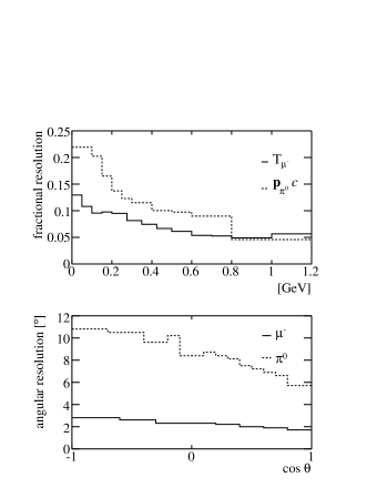
The quality of the reconstruction is assessed by evaluating the residual resolutions of the signal using the MC. Fig. 1 shows the residual resolutions for both the and the . The overall kinetic-energy fractional resolution is 7.4%, and the angular resolution is . The , being a combination of the two fit photons, has an overall momentum resolution of 12.5% and angular resolution of . The energy and momentum resolutions are worse at lower energies and momenta and flatten out toward larger values. The angular resolution is mostly flat and is only slightly better in the forward direction. The angular resolution gets much better in the forward direction as forward going tend to have larger momentum. The resolutions between each particle type are also somewhat correlated. Additionally, the interaction-vertex resolution is 16 cm.
The initial neutrino energy is calculated, assuming that the signal events are from the reaction , from the measured and kinematics under three assumptions: the interaction target is a stationary neutron, the hadronic recoil is a proton, and the neutrino is traveling in the beam direction. Under these assumptions, is constrained even if the proton is unmeasured Nelson (2009). The assumption of a stationary neutron contributes to smearing of the reconstructed neutrino energy because of the neutron’s momentum distribution. The neutrino-energy resolution is 11%. Ideally one would measure the proton, and additional hadronic debris; however, as these particles are rarely above Čerenkov threshold, it is impractical to do so in MiniBooNE. Also, as only 70% of the observable interactions are nucleon-level on neutrons, additional smearing is due to charge-exchanges on protons or other inelastic processes producing a in the final state. These smearings are not expected to be large. The 4-momentum transfer, , to the hadronic system can be calculated from the reconstructed muon and neutrino momentum Nelson (2009). The calculation of the nucleon resonance mass is performed from the neutrino and muon momentum also assuming a stationary neutron (see appendix).
V Event selection
Isolating observable interactions is challenging as such events are expected to comprise only 4% of the data set Casper (2002). The sample is dominated by observable -CCQE (44%), with contributions from observable (19%), and other CC and NC modes. Basic sorting is first performed to separate different classes of events based on their PMT hit distributions. Then the sample is further refined by cutting on reconstructed quantities to yield an observable dominated sample. Each cut is applied and optimized in succession and will be discuss over the remainder of this section.
The detector is triggered by a signal from the Booster accelerator indicating a proton-beam pulse in the Booster neutrino beam line. All activity in the detector is recorded for s starting s before the s neutrino-beam time window. The detector activity is grouped into “subevents:” clusters in time of PMT hits. Groups of 10 or more PMT hits, within a 200 ns window, with time spacings between the hits of no more than 10 ns with at most two spacings less than 20 ns, define a subevent Aguilar-Arevalo et al. (2009). In an ideal neutrino event, the first subevent is always caused by the prompt neutrino interaction; subsequent subevents are due to electrons from stopped-muon decays. Neutrino events with one subevent are primarily due to neutral-current interactions and -CCQE. Two-subevent events are from -CCQE, , and NC. Three-subevent events are almost completely , with some multi- production. Stopped muon decays produce electrons with a maximum energy of 53 MeV which never cause more than 200 PMT hits in the central detector.
To select a sample of contained events, a requirement is made to reject events that penetrate the veto. These events typically cause more than 6 veto PMT hits. Therefore, a two-subevent sample is defined by requiring more than 200 tank PMT hits in the first subevent, fewer than 200 tank PMT hits in the second, and fewer than 6 veto PMT hits for each subevent. The two-subevent sample is predicted to be 71% -CCQE, 16% , and 6% . Observable events make it into the two-subevent sample for several reasons: primarily by and in mineral oil, by fast muon decays whose electrons occur during the prior subevent, and by capture on nucleons affecting 8% of in mineral oil. The two-subevent filter keeps 40% of CCQE and interactions while rejecting 80% of interactions. The rejection of CCQE and signal is mainly from that exit the tank. Additionally, events are lost by the 8% capture rate on carbon.
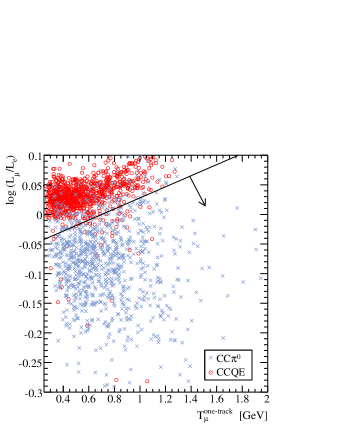
To isolate a purer sample of observable events from the two-subevent sample, before the observable fit is performed, -CCQE events are rejected by cutting on the ratio of the -CCQE fit likelihood to the -CCQE fit likelihood as a function of -fit kinetic energy (see Fig. 2). This cut is motivated by the fact that -CCQE interactions are dominated by a sharp muon ring, while interactions (with the addition of two photon rings) will look “fuzzier” and more electron-like to the fitter. The cut, which has been optimized to reject CCQE, rejects 96% of observable -CCQE while retaining 85% of observable Nelson . Additionally, a reconstructed radius cut of cm is used to constrain events to within the fiducial volume.
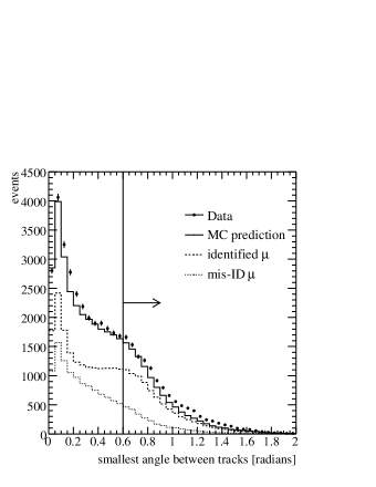
To reject misreconstructed signal events, along with certain backgrounds, a cut is applied to reject events if two of the three Čerenkov rings reconstruct on top of one another. When this occurs the fitter ambiguously divides the total energy between the two tracks. For cases where there are two or fewer rings, the fitter will place two of the tracks in the same direction. For cases where there are three or more Čerenkov rings, the fitter can still get trapped with two tracks on top of one another. This can happen either because of asymmetric decays, a near or below Čerenkov threshold, a dominant ring, or events that truly have overlapping tracks. In all of these cases, the reconstruction becomes poor, especially the identification of the in the event. Fig. 3 shows the smallest reconstructed angle between two of the three reconstructed tracks for both data and MC. The MC events are separated into samples that correctly identified the and those that did not. A cut is optimized on signal events in the MC to reject misidentified , and rejects events with track separations less than 0.6 radians Nelson . This cut reduces the expected misidentification rate to the 20% level. Additionally the observable fraction is increased to 38% and the observable CCQE fraction is reduced to 13%.
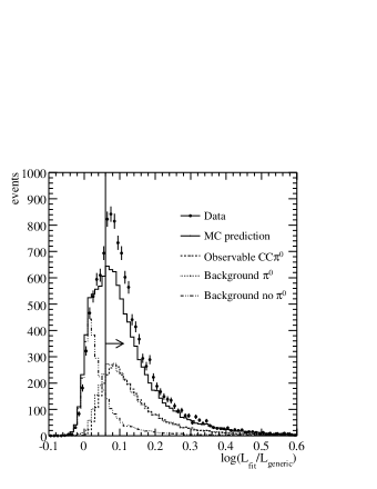
The next series of cuts reject non- backgrounds. The first requirement compares the observable fit likelihood vs. a generic three-track fit and selects events that are more -like. As the observable fit is actually a generic– from a common vertex–fit, this cut selects events that match this criterion. The second cut is on the reconstructed mass about the expected mass. This cut demands that the photons are consistent with a decay. The combination of these cuts define the observable sample. Fig. 4 shows the logarithm of the ratio of the observable fit over the generic three-track fit likelihoods. The MC is separated into three samples: observable , background events with a in the final state or created later in the event, and background events with no . Both the observable and backgrounds with a are more -like than events with no in the event. Additionally, as the backgrounds with a either have multiple pions or the was produced away from the event vertex, the likelihood ratio for these events tend slightly more toward the generic fit. Events with no peak sharply at low ratio values. The optimization rejects non- backgrounds by selecting events greater than 0.06 in this ratio Nelson .
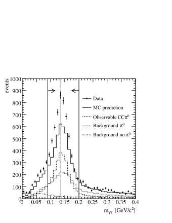
The final cut on the reconstructed mass defines the observable event sample. Fig. 5 shows the reconstructed mass for both data and MC. No assumption is used in the fit that the two photons result from a decay; nevertheless, both data and MC peak at the known mass. The predicted background MC with a in the final state, or a produced after the event, has a broader peak than the signal MC. This broadening occurs for the same reasons discussed for the likelihood ratio; these events either produced a away from the vertex, or there are multiple pions in the final state. As one might expect, background events with no in the final state show no discernible mass peak and pile up at low mass with a long misreconstructed tail extending out to high mass. A cut is optimized to select events around the known mass [0.09 0.2 GeV] to reject non- backgrounds (low mass cut) and to increase signal purity (high mass cut) Nelson . The addition of these selection cuts increases the observable purity to 57% with 6% efficiency.
| cut description | efficiency | purity |
|---|---|---|
| none | 100% | 3.6% |
| Two-subevent and Tank and Veto hits | 38.2% | 5.6% |
| filter and fiducial volume | 27.9% | 29.6% |
| Misreconstruction | 10.3% | 38.1% |
| Likelihood ratio and | 6.4% | 57.0% |
| observable | fraction of | ||
|---|---|---|---|
| mode | description | background | |
| 52.0% | |||
| CCQE | 15.4% | ||
| CCmulti- | 14.0% | ||
| NC- | 8.8% | ||
| others | 9.8% | ||
VI Analysis
The extraction of observable cross sections from the event sample requires a subtraction of background events, corrections for detector effects and cut efficiencies, a well-understood flux, and an estimation of the number of interaction targets. The cross sections are determined by
| (1) |
where is the variable of interest, labels a bin of the measurement, is the bin width, is the number of events in data of bin , is the expected background, is a matrix element that unfolds out detector effects, is the bin efficiency, is the predicted neutrino flux, and is the number of interaction targets. For the single-differential cross-section measurements, the flux factor, , is constant and equals the total flux. For the total cross-section measurement as a function of neutrino energy the flux factor is per energy bin. The extracted cross sections require a detailed understanding of the measurements or predictions of the quantities in Eqn. 1, and their associated systematic uncertainties. By construction, the signal cross-section prediction has minimal impact on the measurements. Wherever the prediction can affect a measurement, usually through the systematic error calculations, the dependence is duly noted.
VI.1 CC backgrounds
The first stage of the cross-section measurement is to subtract the expected background contributions from the measured event rate. This is complicated by the fact that previously measured modes in MiniBooNE (CCQE Aguilar-Arevalo et al. (2010), Aguilar-Arevalo et al. (2010), and Aguilar-Arevalo et al. (2010)) show substantial normalization discrepancies with the Nuance prediction. The single largest background, observable , is well constrained by measurements within the MiniBooNE data set. The observable CCQE in the sample is at a small enough level not warrant further constraint. Most of the remaining backgrounds are unmeasured but individually small.
The backgrounds are important to constrain for two reasons: they contribute the largest single background, and and processes in the mineral oil have large uncertainties. In particular, in mineral oil is, by definition, not an observable because the did not originate in the target nucleus. By tying the observable production to measurements within the MiniBooNE data, the uncertainty on this background can also be further reduced. The total error is separated into an uncertainty on production and an uncertainty on and processes in mineral oil occurring external to the initial target nucleus. Using the high statistics MiniBooNE 3-subevent sample, many measurements of the absolute observable production cross sections have been performed Wilking ; Aguilar-Arevalo et al. (2010). This observable sample is predicted to be 90% pure Wilking ; Aguilar-Arevalo et al. (2010) making it the purest mode measured in the MiniBooNE data set to date. It is a very useful sample for this analysis as the bulk of the background events in the sample fall in the kinematic region well-measured by the observable data. The measurements used are from the tables in Ref. Wilking . Because the re-interaction cross sections for and are strong functions of energy, the constraint on events is applied as a function of kinetic energy and neutrino energy. Fig. 6 shows
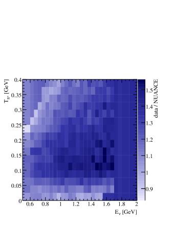
the ratio of the measured observable cross section as a function of and neutrino energies to the Nuance predicted cross section. As the differential cross section with respect to kinetic energy was not reported for bins with small numbers of events, the reweighting function is patched by the ratio of the total observable cross section as a function of neutrino energy. This reweighting factor (as high as 1.6 in some bins) is applied to every observable event in the MC sample. All figures and numbers presented in this article have this reweighting applied. By using the MiniBooNE data to constrain the backgrounds, strict reliance on the Nuance implementation of the Rein-Sehgal model to predict this important background is avoided.
VI.2 Background subtraction
The MC predicts a sample that is 57% pure observable after all analysis cuts. A 23% contribution of observable interactions is set by prior measurements in the MiniBooNE data. The remaining 20% of the event sample is mostly comprised of CCQE and multi- final-state events (see Table 2). These backgrounds, while thought to be produced in larger quantities than the MC prediction, are set by the MC as there is no clear method to extract the normalization of many of these modes from the current data. If the normalizations are different–but on the same order as previously measured modes–they would change the final results by at most a few percent. The uncertainties applied to the production of these backgrounds more than cover the possible normalization differences. After subtracting the backgrounds from the data the sample contains 3725.5 signal events with GeV, which should be compared to 2372.2 predicted events. This is a normalization difference of 1.6, the largest normalization difference that has been observed in the MiniBooNE data thus far. This is attributed to the large effects of pion re-interactions which can directly influence the measured cross section for observable production and the fact that the Nuance prediction appears low even when compared to prior measurements on deuterium data Zeller (2003).
VI.3 Unfolding & flux restriction
To correct for the effects of detector resolution and reconstruction, a method of data unfolding is performed Cowan (1998). The unfolding method constructs a response matrix from the MC that maps reconstructed quantities to their predicted values. The chosen method utilizes the Bayesian technique described in Ref. D’Agostini (1995). This method of data unfolding requires a Bayesian prior for the signal sample, which produces an intrinsic bias. This bias is the only way that the signal cross-section model affects the measured cross sections. In effect, this allows the signal cross-section model to pull the measured cross sections toward the shape of the distributions produced from the model while preserving the normalization measured in the data; nevertheless, strict dependence on the signal cross-section is avoided. For these measurements, the level of uncertainty on the signal model cover the effect of the bias on the central value. For situations where the unfolding is applied to a distribution that is significantly different than the Bayesian prior, the granularity of the unfolding matrix needs to be increased to stabilize the calculation of the systematic uncertainty. Otherwise the uncertainties would be larger than expected due to larger intrinsic bias. For the total cross section as a function of neutrino energy, the unfolding acts on the background-subtracted reconstructed neutrino energy and unfolds back to the neutrino energy prior to the interaction. For each of the flux-averaged differential cross-section measurements, the unfolding acts on the two-dimensional space of neutrino energy and the reconstructed quantity of a particular measurement. For final-state particles, and , the unfolding corrects to the kinematics after final-state effects, and are the least model dependent. For the 4-momentum transfer, , the unfolding extracts to calculated from the initial neutrino and the final-state . In both the total cross section and flux-averaged differential cross section in , the final-state interaction model does bias the measurements. Uncertainties in the signal cross-section model, along with the final-state interaction model, are expected to cover this bias. The unfolded two-dimensional distributions are restricted to a region of unfolded neutrino energy between GeV. This effectively restricts the differential cross-section measurements over the same range of neutrino energy, and flux, as the total cross-section measurement.
VI.4 Efficiency correction
The unfolded distributions are next corrected by a bin-by-bin efficiency. The efficiencies are estimated by taking the ratio of MC signal events after cuts to the predicted distribution of signal events without cuts but restricted to the fiducial volume. The efficiency is insensitive to changes in the underlying MC prediction to within the MC statistical error. While this additional statistical error is not large, it is properly accounted for in the error calculation. The overall efficiency for selecting observable interactions is 6.4%; the bulk of the events () are lost by demanding a that stops and decays in the MiniBooNE tank. The cuts to reduce the backgrounds and preserve well-reconstructed events account for the remainder.
VI.5 Neutrino flux
A major difficulty in extracting absolute cross sections is the need for an accurate flux prediction. The MiniBooNE flux prediction Aguilar-Arevalo et al. (2009) comes strictly from fits to external data Catanesi et al. (2007); Chemakin et al. (2008); Aleshin et al. (1977); Abbott et al. (1992); Allaby et al. ; Dekkers et al. (1965); Eichten et al. (1972); Lundy et al. (1965); Marmer et al. (1969); Vorontsov et al. (1988) and makes no use of the MiniBooNE neutrino data. Fig. 7 shows the predicted flux with systematic uncertainties.

The flux is restricted by the unfolding method to the range 0.5–2.0 GeV, although contributions from the flux outside of this range affect the systematic uncertainties of the unfolding method. The integrated flux over this range is predicted to be /p.o.t./cm2.
VI.6 Number of targets
The Marcol 7 mineral oil is composed of long chains of hydrocarbons. The interaction target is one link in a hydrocarbon chain; chains with an additional hydrogen atom at each end. The molecular weight is the weight of one unit of the chain averaged over the average chain length. The density of the mineral oil is g/cm3 Aguilar-Arevalo et al. (2009). Thermal variations over the course of the run were less than 1%. The fiducial volume is defined to be a sphere 550 cm in radius. Therefore, there are interaction targets.
VII Systematic uncertainties
Sources of systematic uncertainties are separated into two types: flux sources and detector sources. Flux sources affect the number, type, and momentum of the neutrino beam at the detector. Detector sources affect the interaction of neutrinos in the mineral oil and surrounding materials, the interactions of the produced particles with the medium, the creation and propagation of optical photons, and the uncertainties associated with the detector electronics. Whenever possible, the input sources to the systematic uncertainty calculations are fit to both ex-and in-situ data and varied within their full error matrices. These variations are propagated through the entire analysis chain and determine the systematic error separately for each quantity of interest. For sources that affect the number of interactions (e.g. flux and cross-section sources), the central value MC is reweighted by taking the ratio of the value of the underlying parameter’s excursion to that of the central value. This is done to reduce statistical variations in the underlying systematics. Sources that change the properties of an event require separate sets of MC to evaluate the error matrices. The unfortunate aspect of this method is it introduces additional statistical error from the excursion. If the generated sets are large, then this additional error is small.
VII.1 Flux sources
The main sources of flux uncertainties come from particle production and propagation in the Booster neutrino beam line. The proton-beryllium interactions produce , , , and particles that decay into neutrinos. The dominant source of in the flux range of 0.5–2.0 GeV is decay. The production uncertainties are determined by propagating the HARP measurement error matrix by spline interpolation and reweighting into an error matrix describing the contribution of production to the MiniBooNE flux uncertainty Aguilar-Arevalo et al. (2009). Over the flux range of this analysis, the total uncertainty on production introduces a 6.6% uncertainty on the -flux. These uncertainties would be larger if the entire neutrino flux were considered in these measurements; however, as the largest flux uncertainties are in regions of phase space that cannot produce a interaction, it was prudent to restrict the flux range. Horn related uncertainties stem from horn-current variations and skin-depth effects (which mainly affect the high-energy neutrino flux), along with other beam related effects (e.g. secondary interactions), and provide an additional 3.8% uncertainty. No other source contributes more than 0.2% ( production) to the uncertainty. The total uncertainty on the flux over the range 0.5–2.0 GeV, from all flux-related sources, is 7.3%. As the flux prediction affects the measured cross sections through the flux weighting, background subtraction, and unfolding, the resulting uncertainties on the measured total cross section are 7.5% and 7.3% for horn variations and production respectively.
VII.2 Detector sources
Uncertainties associated with the detector result from: neutrino-interaction cross sections, charged-particle interactions in the mineral oil, the creation and interaction of photons in the mineral oil, and the detector read-out electronics. The neutrino-interaction cross sections are varied in Nuance within their error matrices. These variations mainly affect the background predictions; however, the expected signal variations (i.e. flux and signal cross-section variations) do affect the unfolding. The variations of the background cross sections cover the differences seen in the MiniBooNE data; the variations of the signal cover the bias introduced through the chosen unfolding method. The uncertainty on the observable cross section is constrained by measurements within the data Wilking ; Aguilar-Arevalo et al. (2010) assuming no bin-to-bin correlations. The total cross-section uncertainty on the observable cross-section measurement is 5.8%.
The creation and propagation of optical photons in the mineral oil is referred to as the optical model. Several ex-situ measurements were performed on the mineral oil to accurately describe elastic Rayleigh and inelastic Raman scattering, along with the fluorescence components Aguilar-Arevalo et al. (2009); Brown et al. (2006). Additionally, reflections and PMT efficiencies are included in the model, which is defined by a total of 35 correlated parameters. These parameters are varied, in a correlated manner, over a set of data-sized MC samples. The uncertainty calculated from these MC samples contains an additional amount of statistical error; however, in this analysis, the bulk of the additional statistical error is smoothed out by forcing each MC to have the same underlying true distributions. The optical model uncertainty on the total cross-section measurement is 2.8%.
Variations in the detector electronics are estimated as PMT effects. The first measures the PMT response by adjusting the discriminator threshold from 0.1 photoelectrons (PE) to 0.2 PE. The second measures the correlation between the charge and time of the PMT hits. These uncertainties contribute 5.7% and 1.1% to the total cross section respectively.
The dominant uncertainty on the cross-section measurements comes from the uncertainty of and in the mineral oil occurring external to the initial target nucleus where the effects of and internal the target nucleus are included in these measurements. The uncertainty on the cross section on mineral oil is 50% and for it is 35%. The uncertainties come from external data Ashery et al. (1981). These uncertainties affect this measurement to a large degree because of the much larger observable interaction rate (by a factor of 5.2). While this uncertainty is small in the observable cross-section measurements, many that undergo either or in the mineral oil end up in the candidate sample. The uncertainty on the cross sections of and from observable interactions is 12.9%. The uncertainty applied to CC(NC)multi-, , and other backgrounds is included in the background cross-section uncertainties.
VII.3 Discussion
The total systematic uncertainty, from all sources, on the observable total cross-section measurement is 18.7%. The total uncertainty is found by summing all of the individual error matrices. The largest uncertainty, and in the mineral oil, is 12.9%; the flux uncertainties are 10.5%; the remaining detector and neutrino cross-section uncertainties are 8.6%. The total statistical uncertainty is 3.3%. Table 3 summarizes the effects of all sources of systematic uncertainty. Clearly, the limiting factor on the measurement is the understanding of and in mineral oil external to the target nucleus. The two simplest ways to reduce this uncertainty in future experiments are to improve the understanding of pion scattering in a medium, or to use a fine-grained detector that can observe the before the charge-exchange or absorption. Beyond that, gains can always be made from an improved understanding of the incoming neutrino flux.
| source | uncertainty | |
|---|---|---|
| & in mineral oil | 12. | 9% |
| flux | 10. | 5% |
| cross section | 5. | 8% |
| detector electronics | 5. | 8% |
| optical model | 2. | 8% |
| total | 18. | 7% |
VIII Results
This report presents measurements of the observable cross section as a function of neutrino energy, and flux-averaged differential cross sections in , , , , and . These measurements provide the most complete information about this interaction on a nuclear target () at these energies (0.5–2.0 GeV) to date. Great care has been taken to measure cross sections with minimal neutrino-interaction model dependence. First, the definition of an observable interaction limits the dependence of these measurements on the internal and models. Second, most of the measurements are presented in terms of the observed final-state particle kinematics further reducing the dependence of the measurements on the FSI model. Any exceptions to these are noted with the measurements.
The first result, a measurement of the total observable cross section is shown in Fig. 8. This measurement is performed by integrating Eqn. 1 over neutrino energy. This result does contain some dependence on the initial neutrino-interaction model as the unfolding extracts back to the initial neutrino energy; however, this dependence is not expected to be large. The total measured systematic uncertainty is 18.7%, and is slightly higher than the uncertainties presented for the cross sections without this dependence.

The total cross section is higher at all energies than is expected from the combination of the initial interaction Rein and Sehgal (1981) and FSI as implemented in Nuance. An enhancement is also observed in other recent charged-current cross-section measurements Aguilar-Arevalo et al. (2010, 2010); however, the enhancement is a factor of larger than the prediction here.
The differential cross sections provide additional insight into the effect of final-state interactions. By necessity, these cross sections are presented as flux-averaged results due to the low statistics of these measurements. Except for the measurement in , these measurements are mostly independent of the underlying neutrino-interaction model (though there is a slight influence from the unfolding). The flux-averaged cross section, differential in (Fig. 9), is dependent on the initial neutrino-interaction model because it requires knowledge of the initial neutrino kinematics. The measured is unfolded to the calculated from the initial neutrino and final-state muon kinematics. This measurement
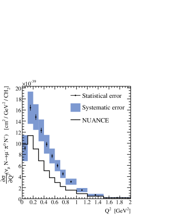
shows an overall enhancement along with a low- suppression (relative to the normalization difference) with a total systematic uncertainty of 16.6%. A similar disagreement is also observed in the cross-section measurement Aguilar-Arevalo et al. (2010).
The kinematics of the are fully specified by its kinetic energy and angle with respect to the incident neutrino beam as the beam is unpolarized. Fig. 10
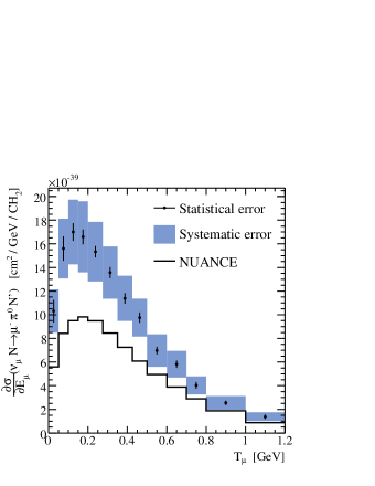
shows the flux-averaged differential cross section in kinetic energy. Like the total cross section, this shows primarily an effect of an overall enhancement of the cross section as the is not expected to be subject to final-state effects. The total systematic uncertainty for this measurement is 15.8%. The flux-averaged differential cross section in - angle (Fig. 11),
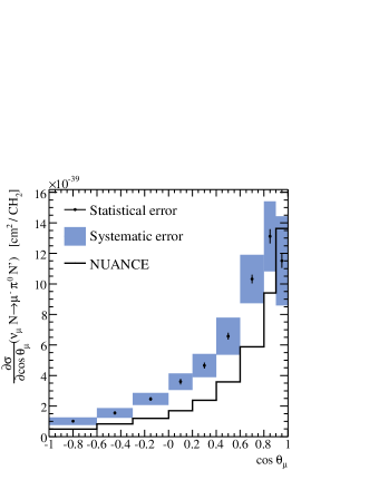
shows a suppression of the cross section at forward angles, characteristic of the low- suppression. As the shapes of the data and the Rein-Sehgal model as implemented in Nuance are fundamentally different in this variable, the unfolding procedure required a reduction of the number of bins in order to be stable. The total systematic uncertainty is 17.4%.
The kinematics yield insight into the final-state interaction effects and are also fully specified by two measurements: the pion momentum and angle with respect to the neutrino beam direction. Fig. 12
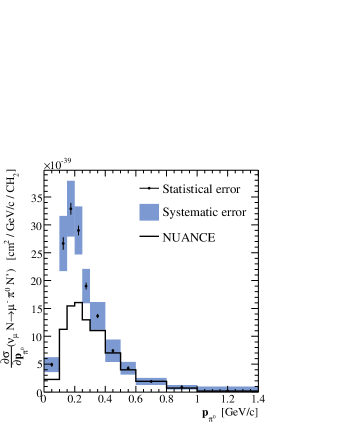
shows the flux-averaged differential cross section in . The cross section is enhanced at low momentum and in the peak, but agrees with the prediction at higher momentum. A similar disagreement is also observed in the cross-section measurements Aguilar-Arevalo et al. (2010). Interactions of both the nucleon resonance and pions with the nuclear medium can cause the ejected to have lower momentum. The total systematic uncertainty is 15.9%. Fig. 13 shows the flux-averaged

differential cross section in - angle. The cross section is more forward than the prediction. The total systematic error is 16.3%.
Each of the cross-section measurements also provide a measurement of the flux-averaged total cross section. From these total cross sections, all of the observable cross-section measurements can be compared. Table 4
| measurement | [cm2] | |
|---|---|---|
| 9.05 | 1.44 | |
| 9.28 | 1.55 | |
| 9.20 | 1.47 | |
| 9.10 | 1.50 | |
| 9.03 | 1.54 | |
| 9.54 | 1.55 | |
| 9.20 | 1.51 | |
shows the flux-averaged total cross sections calculated from each measurement. The measurements all agree within 6%, well within the uncertainty. While all measurements use the same data, small differences can result from biases due to the efficiencies and unfoldings. The results are combined in a simple average, assuming 100% correlated uncertainties, to yield cm2/ at flux-averaged neutrino energy of GeV. The averaged flux-averaged total cross-section measurement is found to be a factor of higher than the Nuance prediction.
IX Conclusion
The measurements presented here provide the most complete understanding of interactions at energies below 2 GeV to date. They are the first on a nuclear target (), at these energies, and provide differential cross-section measurements in terms of the final state, non-nuclear, particle kinematics. The development of a novel 3-Čerenkov ring fitter has facilitated the reconstruction of both the and in a interaction. This reconstruction allows for the measurement of the full kinematics of the event providing for the measurement of six cross sections: the total cross section as a function of neutrino energy, and flux-averaged differential cross sections in , , , , and . These cross sections show an enhancement over the initial interaction model Rein and Sehgal (1981) and FSI effects as implemented in Nuance. The flux-averaged total cross section is measured to be cm2/ at mean neutrino energy of GeV. These measurements should prove useful for understanding incoherent pion production on nuclear targets.
Acknowledgements.
The authors would like to acknowledge the support of Fermilab, the Department of Energy, and the National Science Foundation in the construction, operation, and data analysis of the Mini Booster Neutrino Experiment.*
Appendix A Hadronic invariant mass
The background-subtracted reconstructed nucleon resonance mass is calculable from the reconstructed neutrino and muon 4-momenta. Fig. 14 shows the background-subtracted reconstructed
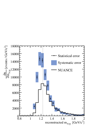
invariant mass for data and the MC expectation. The data has not been corrected for cut efficiencies. The fact that the data peaks somewhat below the resonance while Nuance peaks at the resonance implies the model is not properly taking into account final state interaction effects; however, it is observed that the MiniBooNE data is almost completed dominated by the resonance. This shift can also be interpreted as an effective change in the recoil mass, , of the hadronic system. Additionally, it has been verified that CCQE interactions, which do not involve a resonance, peak at threshold (not displayed).
Appendix B Tables
The tables presented in this appendix are provided to quantify the flux, Fig. 7, and the cross-section measurements, Figs. 8, 9, 10, 11, 12, and 13.
| Bin edge [GeV] | 0. | 50 | 0. | 60 | 0. | 70 | 0. | 80 | 0. | 90 | 1. | 00 | 1. | 10 | 1. | 20 | 1. | 30 | 1. | 40 | 1. | 50 | 1. | 60 | 1. | 70 | 1.80-2.00 | |
|---|---|---|---|---|---|---|---|---|---|---|---|---|---|---|---|---|---|---|---|---|---|---|---|---|---|---|---|---|
| CV [/p.o.t./cm2/GeV] | 4. | 57 | 4. | 53 | 4. | 37 | 4. | 07 | 3. | 68 | 3. | 24 | 2. | 76 | 2. | 26 | 1. | 79 | 1. | 36 | 1. | 00 | 0. | 72 | 0. | 51 | 0. | 30 |
| Total Syst. | 0. | 33 | 0. | 26 | 0. | 25 | 0. | 26 | 0. | 22 | 0. | 18 | 0. | 20 | 0. | 28 | 0. | 24 | 0. | 17 | 0. | 13 | 0. | 12 | 0. | 10 | 0. | 07 |
| 0.50 | 1. | 00 | 0. | 91 | 0. | 91 | 0. | 79 | 0. | 77 | 0. | 45 | -0. | 06 | -0. | 35 | -0. | 33 | -0. | 12 | 0. | 12 | 0. | 19 | 0. | 25 | 0. | 28 |
| 0.60 | 0. | 91 | 1. | 00 | 0. | 92 | 0. | 80 | 0. | 77 | 0. | 54 | 0. | 08 | -0. | 16 | -0. | 16 | -0. | 01 | 0. | 13 | 0. | 15 | 0. | 17 | 0. | 18 |
| 0.70 | 0. | 91 | 0. | 92 | 1. | 00 | 0. | 87 | 0. | 86 | 0. | 61 | 0. | 13 | -0. | 19 | -0. | 18 | 0. | 04 | 0. | 25 | 0. | 28 | 0. | 31 | 0. | 33 |
| 0.80 | 0. | 79 | 0. | 80 | 0. | 87 | 1. | 00 | 0. | 92 | 0. | 69 | 0. | 15 | -0. | 17 | -0. | 17 | 0. | 09 | 0. | 35 | 0. | 40 | 0. | 41 | 0. | 44 |
| 0.90 | 0. | 77 | 0. | 77 | 0. | 86 | 0. | 92 | 1. | 00 | 0. | 83 | 0. | 34 | -0. | 02 | -0. | 01 | 0. | 23 | 0. | 44 | 0. | 47 | 0. | 49 | 0. | 50 |
| 1.00 | 0. | 45 | 0. | 54 | 0. | 61 | 0. | 69 | 0. | 83 | 1. | 00 | 0. | 75 | 0. | 46 | 0. | 44 | 0. | 60 | 0. | 65 | 0. | 62 | 0. | 57 | 0. | 55 |
| 1.10 | -0. | 06 | 0. | 08 | 0. | 13 | 0. | 15 | 0. | 34 | 0. | 75 | 1. | 00 | 0. | 89 | 0. | 87 | 0. | 87 | 0. | 70 | 0. | 58 | 0. | 47 | 0. | 38 |
| 1.20 | -0. | 35 | -0. | 16 | -0. | 19 | -0. | 17 | -0. | 02 | 0. | 46 | 0. | 89 | 1. | 00 | 0. | 98 | 0. | 84 | 0. | 54 | 0. | 40 | 0. | 28 | 0. | 19 |
| 1.30 | -0. | 33 | -0. | 16 | -0. | 18 | -0. | 17 | -0. | 01 | 0. | 44 | 0. | 87 | 0. | 98 | 1. | 00 | 0. | 91 | 0. | 63 | 0. | 49 | 0. | 38 | 0. | 26 |
| 1.40 | -0. | 12 | -0. | 01 | 0. | 04 | 0. | 09 | 0. | 23 | 0. | 60 | 0. | 87 | 0. | 84 | 0. | 91 | 1. | 00 | 0. | 89 | 0. | 78 | 0. | 66 | 0. | 53 |
| 1.50 | 0. | 12 | 0. | 13 | 0. | 25 | 0. | 35 | 0. | 44 | 0. | 65 | 0. | 70 | 0. | 54 | 0. | 63 | 0. | 89 | 1. | 00 | 0. | 97 | 0. | 89 | 0. | 79 |
| 1.60 | 0. | 19 | 0. | 15 | 0. | 28 | 0. | 40 | 0. | 47 | 0. | 62 | 0. | 58 | 0. | 40 | 0. | 49 | 0. | 78 | 0. | 97 | 1. | 00 | 0. | 97 | 0. | 91 |
| 1.70 | 0. | 25 | 0. | 17 | 0. | 31 | 0. | 41 | 0. | 49 | 0. | 57 | 0. | 47 | 0. | 28 | 0. | 38 | 0. | 66 | 0. | 89 | 0. | 97 | 1. | 00 | 0. | 97 |
| 1.80-2.00 | 0. | 28 | 0. | 18 | 0. | 33 | 0. | 44 | 0. | 50 | 0. | 55 | 0. | 38 | 0. | 19 | 0. | 26 | 0. | 53 | 0. | 79 | 0. | 91 | 0. | 97 | 1. | 00 |
| Bin edge [GeV] | 0. | 50 | 0. | 60 | 0. | 70 | 0. | 80 | 0. | 90 | 1. | 00 | 1. | 10 | 1. | 20 | 1. | 30 | 1. | 40 | 1. | 50 | 1. | 60 | 1. | 70 | 1.80-2.00 | |
|---|---|---|---|---|---|---|---|---|---|---|---|---|---|---|---|---|---|---|---|---|---|---|---|---|---|---|---|---|
| CV [cm2] | 1. | 76 | 3. | 83 | 5. | 68 | 7. | 31 | 9. | 20 | 11. | 06 | 12. | 42 | 13. | 89 | 15. | 23 | 16. | 38 | 18. | 20 | 19. | 37 | 20. | 80 | 21. | 92 |
| Stat. | 0. | 18 | 0. | 23 | 0. | 26 | 0. | 29 | 0. | 34 | 0. | 41 | 0. | 49 | 0. | 60 | 0. | 74 | 0. | 92 | 1. | 24 | 1. | 62 | 2. | 16 | 2. | 24 |
| Total Syst. | 0. | 49 | 0. | 78 | 0. | 97 | 1. | 17 | 1. | 50 | 1. | 85 | 2. | 16 | 2. | 46 | 2. | 82 | 3. | 17 | 3. | 61 | 4. | 15 | 4. | 49 | 5. | 26 |
| 0.50 | 1. | 00 | 0. | 93 | 0. | 80 | 0. | 74 | 0. | 71 | 0. | 77 | 0. | 74 | 0. | 68 | 0. | 63 | 0. | 59 | 0. | 50 | 0. | 50 | 0. | 49 | 0. | 54 |
| 0.60 | 0. | 93 | 1. | 00 | 0. | 96 | 0. | 90 | 0. | 88 | 0. | 86 | 0. | 81 | 0. | 79 | 0. | 72 | 0. | 68 | 0. | 62 | 0. | 56 | 0. | 59 | 0. | 59 |
| 0.70 | 0. | 80 | 0. | 96 | 1. | 00 | 0. | 98 | 0. | 96 | 0. | 92 | 0. | 85 | 0. | 86 | 0. | 79 | 0. | 75 | 0. | 73 | 0. | 64 | 0. | 68 | 0. | 65 |
| 0.80 | 0. | 74 | 0. | 90 | 0. | 98 | 1. | 00 | 0. | 99 | 0. | 96 | 0. | 91 | 0. | 91 | 0. | 87 | 0. | 84 | 0. | 81 | 0. | 75 | 0. | 77 | 0. | 74 |
| 0.90 | 0. | 71 | 0. | 88 | 0. | 96 | 0. | 99 | 1. | 00 | 0. | 97 | 0. | 93 | 0. | 94 | 0. | 89 | 0. | 86 | 0. | 85 | 0. | 77 | 0. | 80 | 0. | 75 |
| 1.00 | 0. | 77 | 0. | 86 | 0. | 92 | 0. | 96 | 0. | 97 | 1. | 00 | 0. | 99 | 0. | 98 | 0. | 95 | 0. | 92 | 0. | 89 | 0. | 85 | 0. | 86 | 0. | 83 |
| 1.10 | 0. | 74 | 0. | 81 | 0. | 85 | 0. | 91 | 0. | 93 | 0. | 99 | 1. | 00 | 0. | 99 | 0. | 97 | 0. | 96 | 0. | 91 | 0. | 91 | 0. | 90 | 0. | 89 |
| 1.20 | 0. | 68 | 0. | 79 | 0. | 86 | 0. | 91 | 0. | 94 | 0. | 98 | 0. | 99 | 1. | 00 | 0. | 99 | 0. | 97 | 0. | 95 | 0. | 91 | 0. | 92 | 0. | 89 |
| 1.30 | 0. | 63 | 0. | 72 | 0. | 79 | 0. | 87 | 0. | 89 | 0. | 95 | 0. | 97 | 0. | 99 | 1. | 00 | 0. | 99 | 0. | 97 | 0. | 96 | 0. | 95 | 0. | 94 |
| 1.40 | 0. | 59 | 0. | 68 | 0. | 75 | 0. | 84 | 0. | 86 | 0. | 92 | 0. | 96 | 0. | 97 | 0. | 99 | 1. | 00 | 0. | 98 | 0. | 98 | 0. | 97 | 0. | 96 |
| 1.50 | 0. | 50 | 0. | 62 | 0. | 73 | 0. | 81 | 0. | 85 | 0. | 89 | 0. | 91 | 0. | 95 | 0. | 97 | 0. | 98 | 1. | 00 | 0. | 97 | 0. | 97 | 0. | 94 |
| 1.60 | 0. | 50 | 0. | 56 | 0. | 64 | 0. | 75 | 0. | 77 | 0. | 85 | 0. | 91 | 0. | 91 | 0. | 96 | 0. | 98 | 0. | 97 | 1. | 00 | 0. | 97 | 0. | 98 |
| 1.70 | 0. | 49 | 0. | 59 | 0. | 68 | 0. | 77 | 0. | 80 | 0. | 86 | 0. | 90 | 0. | 92 | 0. | 95 | 0. | 97 | 0. | 97 | 0. | 97 | 1. | 00 | 0. | 97 |
| 1.80-2.00 | 0. | 54 | 0. | 59 | 0. | 65 | 0. | 74 | 0. | 75 | 0. | 83 | 0. | 89 | 0. | 89 | 0. | 94 | 0. | 96 | 0. | 94 | 0. | 98 | 0. | 97 | 1. | 00 |
| Bin edge [GeV2] | 0. | 00 | 0. | 10 | 0. | 20 | 0. | 30 | 0. | 40 | 0. | 50 | 0. | 60 | 0. | 70 | 0. | 80 | 1. | 00 | 1. | 20 | 1.50-2.00 | |
|---|---|---|---|---|---|---|---|---|---|---|---|---|---|---|---|---|---|---|---|---|---|---|---|---|
| CV [cm2/GeV2] | 9. | 12 | 16. | 41 | 14. | 72 | 12. | 32 | 9. | 82 | 7. | 70 | 5. | 97 | 4. | 48 | 3. | 07 | 1. | 55 | 0. | 70 | 0. | 18 |
| Stat. | 0. | 39 | 0. | 52 | 0. | 49 | 0. | 45 | 0. | 41 | 0. | 36 | 0. | 33 | 0. | 30 | 0. | 17 | 0. | 12 | 0. | 07 | 0. | 02 |
| Total Syst. | 2. | 33 | 2. | 90 | 2. | 31 | 1. | 96 | 1. | 68 | 1. | 33 | 1. | 00 | 0. | 75 | 0. | 55 | 0. | 36 | 0. | 18 | 0. | 07 |
| 0.00 | 1. | 00 | 0. | 94 | 0. | 95 | 0. | 91 | 0. | 78 | 0. | 78 | 0. | 87 | 0. | 84 | 0. | 83 | 0. | 70 | 0. | 71 | 0. | 60 |
| 0.10 | 0. | 94 | 1. | 00 | 0. | 94 | 0. | 90 | 0. | 66 | 0. | 68 | 0. | 91 | 0. | 78 | 0. | 81 | 0. | 61 | 0. | 66 | 0. | 62 |
| 0.20 | 0. | 95 | 0. | 94 | 1. | 00 | 0. | 97 | 0. | 83 | 0. | 84 | 0. | 90 | 0. | 82 | 0. | 79 | 0. | 76 | 0. | 70 | 0. | 53 |
| 0.30 | 0. | 91 | 0. | 90 | 0. | 97 | 1. | 00 | 0. | 81 | 0. | 83 | 0. | 93 | 0. | 73 | 0. | 70 | 0. | 76 | 0. | 60 | 0. | 41 |
| 0.40 | 0. | 78 | 0. | 66 | 0. | 83 | 0. | 81 | 1. | 00 | 0. | 99 | 0. | 67 | 0. | 81 | 0. | 70 | 0. | 89 | 0. | 72 | 0. | 37 |
| 0.50 | 0. | 78 | 0. | 68 | 0. | 84 | 0. | 83 | 0. | 99 | 1. | 00 | 0. | 73 | 0. | 79 | 0. | 68 | 0. | 91 | 0. | 69 | 0. | 34 |
| 0.60 | 0. | 87 | 0. | 91 | 0. | 90 | 0. | 93 | 0. | 67 | 0. | 73 | 1. | 00 | 0. | 71 | 0. | 72 | 0. | 69 | 0. | 60 | 0. | 49 |
| 0.70 | 0. | 84 | 0. | 78 | 0. | 82 | 0. | 73 | 0. | 81 | 0. | 79 | 0. | 71 | 1. | 00 | 0. | 97 | 0. | 77 | 0. | 91 | 0. | 78 |
| 0.80 | 0. | 83 | 0. | 81 | 0. | 79 | 0. | 70 | 0. | 70 | 0. | 68 | 0. | 72 | 0. | 97 | 1. | 00 | 0. | 72 | 0. | 93 | 0. | 87 |
| 1.00 | 0. | 70 | 0. | 61 | 0. | 76 | 0. | 76 | 0. | 89 | 0. | 91 | 0. | 69 | 0. | 77 | 0. | 72 | 1. | 00 | 0. | 80 | 0. | 43 |
| 1.20 | 0. | 71 | 0. | 66 | 0. | 70 | 0. | 60 | 0. | 72 | 0. | 69 | 0. | 60 | 0. | 91 | 0. | 93 | 0. | 80 | 1. | 00 | 0. | 87 |
| 1.50-2.00 | 0. | 60 | 0. | 62 | 0. | 53 | 0. | 41 | 0. | 37 | 0. | 34 | 0. | 49 | 0. | 78 | 0. | 87 | 0. | 43 | 0. | 87 | 1. | 00 |
| Bin edge [GeV] | 0. | 00 | 0. | 05 | 0. | 10 | 0. | 15 | 0. | 20 | 0. | 28 | 0. | 35 | 0. | 42 | 0. | 50 | 0. | 60 | 0. | 70 | 0. | 80 | 1.00-1.20 | |
| CV [cm2/GeV] | 10. | 31 | 15. | 60 | 17. | 00 | 16. | 58 | 15. | 33 | 13. | 57 | 11. | 38 | 9. | 76 | 6. | 97 | 5. | 82 | 4. | 03 | 2. | 55 | 1. | 38 |
| Stat. | 0. | 96 | 1. | 03 | 0. | 75 | 0. | 63 | 0. | 48 | 0. | 47 | 0. | 45 | 0. | 43 | 0. | 32 | 0. | 32 | 0. | 28 | 0. | 19 | 0. | 21 |
| Total Syst. | 1. | 83 | 2. | 52 | 2. | 73 | 3. | 00 | 2. | 52 | 2. | 21 | 1. | 91 | 1. | 60 | 1. | 38 | 1. | 12 | 0. | 76 | 0. | 58 | 0. | 36 |
| 0.00 | 1. | 00 | 0. | 50 | 0. | 75 | 0. | 70 | 0. | 66 | 0. | 82 | 0. | 75 | 0. | 65 | 0. | 76 | 0. | 89 | 0. | 62 | 0. | 31 | 0. | 34 |
| 0.05 | 0. | 50 | 1. | 00 | 0. | 87 | 0. | 83 | 0. | 88 | 0. | 78 | 0. | 80 | 0. | 85 | 0. | 67 | 0. | 57 | 0. | 86 | 0. | 78 | 0. | 56 |
| 0.10 | 0. | 75 | 0. | 87 | 1. | 00 | 0. | 93 | 0. | 91 | 0. | 92 | 0. | 92 | 0. | 90 | 0. | 85 | 0. | 82 | 0. | 87 | 0. | 67 | 0. | 51 |
| 0.15 | 0. | 70 | 0. | 83 | 0. | 93 | 1. | 00 | 0. | 83 | 0. | 90 | 0. | 87 | 0. | 90 | 0. | 91 | 0. | 81 | 0. | 90 | 0. | 61 | 0. | 42 |
| 0.20 | 0. | 66 | 0. | 88 | 0. | 91 | 0. | 83 | 1. | 00 | 0. | 91 | 0. | 93 | 0. | 90 | 0. | 75 | 0. | 77 | 0. | 87 | 0. | 84 | 0. | 70 |
| 0.28 | 0. | 82 | 0. | 78 | 0. | 92 | 0. | 90 | 0. | 91 | 1. | 00 | 0. | 95 | 0. | 91 | 0. | 91 | 0. | 92 | 0. | 88 | 0. | 66 | 0. | 58 |
| 0.35 | 0. | 75 | 0. | 80 | 0. | 92 | 0. | 87 | 0. | 93 | 0. | 95 | 1. | 00 | 0. | 93 | 0. | 85 | 0. | 87 | 0. | 88 | 0. | 75 | 0. | 65 |
| 0.42 | 0. | 65 | 0. | 85 | 0. | 90 | 0. | 90 | 0. | 90 | 0. | 91 | 0. | 93 | 1. | 00 | 0. | 89 | 0. | 78 | 0. | 92 | 0. | 79 | 0. | 57 |
| 0.50 | 0. | 76 | 0. | 67 | 0. | 85 | 0. | 91 | 0. | 75 | 0. | 91 | 0. | 85 | 0. | 89 | 1. | 00 | 0. | 89 | 0. | 84 | 0. | 53 | 0. | 38 |
| 0.60 | 0. | 89 | 0. | 57 | 0. | 82 | 0. | 81 | 0. | 77 | 0. | 92 | 0. | 87 | 0. | 78 | 0. | 89 | 1. | 00 | 0. | 78 | 0. | 47 | 0. | 45 |
| 0.70 | 0. | 62 | 0. | 86 | 0. | 87 | 0. | 90 | 0. | 87 | 0. | 88 | 0. | 88 | 0. | 92 | 0. | 84 | 0. | 78 | 1. | 00 | 0. | 77 | 0. | 55 |
| 0.80 | 0. | 31 | 0. | 78 | 0. | 67 | 0. | 61 | 0. | 84 | 0. | 66 | 0. | 75 | 0. | 79 | 0. | 53 | 0. | 47 | 0. | 77 | 1. | 00 | 0. | 72 |
| 1.00-1.20 | 0. | 34 | 0. | 56 | 0. | 51 | 0. | 42 | 0. | 70 | 0. | 58 | 0. | 65 | 0. | 57 | 0. | 38 | 0. | 45 | 0. | 55 | 0. | 72 | 1. | 00 |
| Bin edge | -1. | 00 | -0. | 60 | -0. | 30 | 0. | 00 | 0. | 20 | 0. | 40 | 0. | 60 | 0. | 80 | 0.90-1.00 | |
|---|---|---|---|---|---|---|---|---|---|---|---|---|---|---|---|---|---|---|
| CV [cm2] | 1. | 01 | 1. | 55 | 2. | 46 | 3. | 60 | 4. | 65 | 6. | 58 | 10. | 32 | 13. | 11 | 11. | 51 |
| Stat. | 0. | 08 | 0. | 11 | 0. | 13 | 0. | 18 | 0. | 19 | 0. | 23 | 0. | 28 | 0. | 47 | 0. | 46 |
| Total Syst. | 0. | 25 | 0. | 32 | 0. | 40 | 0. | 54 | 0. | 76 | 1. | 22 | 1. | 59 | 2. | 29 | 2. | 92 |
| -1.00 | 1. | 00 | 0. | 61 | 0. | 67 | 0. | 45 | 0. | 58 | 0. | 86 | 0. | 34 | 0. | 66 | 0. | 53 |
| -0.60 | 0. | 61 | 1. | 00 | 0. | 84 | 0. | 63 | 0. | 87 | 0. | 77 | 0. | 70 | 0. | 84 | 0. | 71 |
| -0.30 | 0. | 67 | 0. | 84 | 1. | 00 | 0. | 78 | 0. | 90 | 0. | 83 | 0. | 80 | 0. | 92 | 0. | 83 |
| 0.00 | 0. | 45 | 0. | 63 | 0. | 78 | 1. | 00 | 0. | 76 | 0. | 64 | 0. | 90 | 0. | 80 | 0. | 87 |
| 0.20 | 0. | 58 | 0. | 87 | 0. | 90 | 0. | 76 | 1. | 00 | 0. | 79 | 0. | 84 | 0. | 92 | 0. | 84 |
| 0.40 | 0. | 86 | 0. | 77 | 0. | 83 | 0. | 64 | 0. | 79 | 1. | 00 | 0. | 60 | 0. | 87 | 0. | 76 |
| 0.60 | 0. | 34 | 0. | 70 | 0. | 80 | 0. | 90 | 0. | 84 | 0. | 60 | 1. | 00 | 0. | 84 | 0. | 92 |
| 0.80 | 0. | 66 | 0. | 84 | 0. | 92 | 0. | 80 | 0. | 92 | 0. | 87 | 0. | 84 | 1. | 00 | 0. | 92 |
| 0.90-1.00 | 0. | 53 | 0. | 71 | 0. | 83 | 0. | 87 | 0. | 84 | 0. | 76 | 0. | 92 | 0. | 92 | 1. | 00 |
| Bin edge [GeV/] | 0. | 00 | 0. | 10 | 0. | 15 | 0. | 20 | 0. | 25 | 0. | 30 | 0. | 40 | 0. | 50 | 0. | 60 | 0. | 80 | 1.00-1.40 | |
|---|---|---|---|---|---|---|---|---|---|---|---|---|---|---|---|---|---|---|---|---|---|---|
| CV [cm2/GeV/] | 4. | 92 | 26. | 65 | 32. | 90 | 28. | 99 | 19. | 02 | 13. | 65 | 7. | 41 | 4. | 27 | 1. | 90 | 0. | 87 | 0. | 19 |
| Stat. | 0. | 37 | 1. | 10 | 1. | 05 | 0. | 87 | 0. | 61 | 0. | 37 | 0. | 31 | 0. | 33 | 0. | 25 | 0. | 35 | 0. | 21 |
| Total Syst. | 1. | 34 | 4. | 94 | 5. | 00 | 4. | 31 | 3. | 09 | 2. | 49 | 2. | 01 | 1. | 14 | 0. | 63 | 0. | 40 | 0. | 79 |
| 0.00 | 1. | 00 | 0. | 74 | 0. | 83 | 0. | 52 | 0. | 82 | 0. | 79 | 0. | 47 | 0. | 25 | 0. | 26 | 0. | 44 | 0. | 02 |
| 0.10 | 0. | 74 | 1. | 00 | 0. | 92 | 0. | 74 | 0. | 90 | 0. | 70 | 0. | 30 | 0. | 51 | 0. | 58 | 0. | 26 | -0. | 41 |
| 0.15 | 0. | 83 | 0. | 92 | 1. | 00 | 0. | 85 | 0. | 97 | 0. | 88 | 0. | 56 | 0. | 59 | 0. | 57 | 0. | 36 | -0. | 14 |
| 0.20 | 0. | 52 | 0. | 74 | 0. | 85 | 1. | 00 | 0. | 82 | 0. | 84 | 0. | 73 | 0. | 84 | 0. | 72 | 0. | 26 | 0. | 05 |
| 0.25 | 0. | 82 | 0. | 90 | 0. | 97 | 0. | 82 | 1. | 00 | 0. | 90 | 0. | 55 | 0. | 61 | 0. | 63 | 0. | 38 | -0. | 16 |
| 0.30 | 0. | 79 | 0. | 70 | 0. | 88 | 0. | 84 | 0. | 90 | 1. | 00 | 0. | 84 | 0. | 69 | 0. | 57 | 0. | 48 | 0. | 24 |
| 0.40 | 0. | 47 | 0. | 30 | 0. | 56 | 0. | 73 | 0. | 55 | 0. | 84 | 1. | 00 | 0. | 72 | 0. | 46 | 0. | 44 | 0. | 63 |
| 0.50 | 0. | 25 | 0. | 51 | 0. | 59 | 0. | 84 | 0. | 61 | 0. | 69 | 0. | 72 | 1. | 00 | 0. | 89 | 0. | 35 | 0. | 08 |
| 0.60 | 0. | 26 | 0. | 58 | 0. | 57 | 0. | 72 | 0. | 63 | 0. | 57 | 0. | 46 | 0. | 89 | 1. | 00 | 0. | 39 | -0. | 19 |
| 0.80 | 0. | 44 | 0. | 26 | 0. | 36 | 0. | 26 | 0. | 38 | 0. | 48 | 0. | 44 | 0. | 35 | 0. | 39 | 1. | 00 | 0. | 24 |
| 1.00-1.40 | 0. | 02 | -0. | 41 | -0. | 14 | 0. | 05 | -0. | 16 | 0. | 24 | 0. | 63 | 0. | 08 | -0. | 19 | 0. | 24 | 1. | 00 |
| Bin edge | -1. | 00 | -0. | 70 | -0. | 40 | -0. | 20 | -0. | 10 | 0. | 00 | 0. | 10 | 0. | 20 | 0. | 30 | 0. | 40 | 0. | 50 | 0. | 60 | 0. | 70 | 0. | 80 | 0.90-1.00 | |
|---|---|---|---|---|---|---|---|---|---|---|---|---|---|---|---|---|---|---|---|---|---|---|---|---|---|---|---|---|---|---|
| CV [cm2] | 2. | 34 | 2. | 45 | 2. | 83 | 2. | 76 | 2. | 77 | 3. | 06 | 3. | 55 | 4. | 01 | 4. | 57 | 5. | 47 | 6. | 44 | 7. | 66 | 9. | 14 | 11. | 36 | 14. | 59 |
| Stat. | 0. | 16 | 0. | 12 | 0. | 14 | 0. | 18 | 0. | 17 | 0. | 18 | 0. | 19 | 0. | 21 | 0. | 22 | 0. | 26 | 0. | 29 | 0. | 33 | 0. | 39 | 0. | 49 | 0. | 66 |
| Total Syst. | 0. | 44 | 0. | 45 | 0. | 50 | 0. | 46 | 0. | 49 | 0. | 59 | 0. | 60 | 0. | 69 | 0. | 76 | 0. | 95 | 1. | 05 | 1. | 26 | 1. | 48 | 2. | 08 | 2. | 83 |
| -1.00 | 1. | 00 | 0. | 87 | 0. | 78 | 0. | 78 | 0. | 84 | 0. | 62 | 0. | 85 | 0. | 84 | 0. | 78 | 0. | 85 | 0. | 81 | 0. | 86 | 0. | 80 | 0. | 63 | 0. | 81 |
| -0.70 | 0. | 87 | 1. | 00 | 0. | 70 | 0. | 78 | 0. | 87 | 0. | 63 | 0. | 91 | 0. | 81 | 0. | 71 | 0. | 92 | 0. | 86 | 0. | 88 | 0. | 80 | 0. | 60 | 0. | 88 |
| -0.40 | 0. | 78 | 0. | 70 | 1. | 00 | 0. | 67 | 0. | 69 | 0. | 48 | 0. | 76 | 0. | 93 | 0. | 86 | 0. | 71 | 0. | 70 | 0. | 80 | 0. | 80 | 0. | 60 | 0. | 68 |
| -0.20 | 0. | 78 | 0. | 78 | 0. | 67 | 1. | 00 | 0. | 96 | 0. | 92 | 0. | 90 | 0. | 75 | 0. | 82 | 0. | 84 | 0. | 93 | 0. | 89 | 0. | 90 | 0. | 90 | 0. | 84 |
| -0.10 | 0. | 84 | 0. | 87 | 0. | 69 | 0. | 96 | 1. | 00 | 0. | 88 | 0. | 95 | 0. | 80 | 0. | 82 | 0. | 91 | 0. | 94 | 0. | 91 | 0. | 89 | 0. | 82 | 0. | 90 |
| 0.00 | 0. | 62 | 0. | 63 | 0. | 48 | 0. | 92 | 0. | 88 | 1. | 00 | 0. | 80 | 0. | 59 | 0. | 75 | 0. | 72 | 0. | 87 | 0. | 77 | 0. | 81 | 0. | 90 | 0. | 75 |
| 0.10 | 0. | 85 | 0. | 91 | 0. | 76 | 0. | 90 | 0. | 95 | 0. | 80 | 1. | 00 | 0. | 89 | 0. | 84 | 0. | 95 | 0. | 93 | 0. | 94 | 0. | 91 | 0. | 77 | 0. | 93 |
| 0.20 | 0. | 84 | 0. | 81 | 0. | 93 | 0. | 75 | 0. | 80 | 0. | 59 | 0. | 89 | 1. | 00 | 0. | 92 | 0. | 85 | 0. | 83 | 0. | 88 | 0. | 87 | 0. | 68 | 0. | 82 |
| 0.30 | 0. | 78 | 0. | 71 | 0. | 86 | 0. | 82 | 0. | 82 | 0. | 75 | 0. | 84 | 0. | 92 | 1. | 00 | 0. | 80 | 0. | 86 | 0. | 87 | 0. | 90 | 0. | 83 | 0. | 80 |
| 0.40 | 0. | 85 | 0. | 92 | 0. | 71 | 0. | 84 | 0. | 91 | 0. | 72 | 0. | 95 | 0. | 85 | 0. | 80 | 1. | 00 | 0. | 92 | 0. | 92 | 0. | 87 | 0. | 71 | 0. | 95 |
| 0.50 | 0. | 81 | 0. | 86 | 0. | 70 | 0. | 93 | 0. | 94 | 0. | 87 | 0. | 93 | 0. | 83 | 0. | 86 | 0. | 92 | 1. | 00 | 0. | 95 | 0. | 93 | 0. | 88 | 0. | 92 |
| 0.60 | 0. | 86 | 0. | 88 | 0. | 80 | 0. | 89 | 0. | 91 | 0. | 77 | 0. | 94 | 0. | 88 | 0. | 87 | 0. | 92 | 0. | 95 | 1. | 00 | 0. | 95 | 0. | 81 | 0. | 93 |
| 0.70 | 0. | 80 | 0. | 80 | 0. | 80 | 0. | 90 | 0. | 89 | 0. | 81 | 0. | 91 | 0. | 87 | 0. | 90 | 0. | 87 | 0. | 93 | 0. | 95 | 1. | 00 | 0. | 88 | 0. | 90 |
| 0.80 | 0. | 63 | 0. | 60 | 0. | 60 | 0. | 90 | 0. | 82 | 0. | 90 | 0. | 77 | 0. | 68 | 0. | 83 | 0. | 71 | 0. | 88 | 0. | 81 | 0. | 88 | 1. | 00 | 0. | 77 |
| 0.90-1.00 | 0. | 81 | 0. | 88 | 0. | 68 | 0. | 84 | 0. | 90 | 0. | 75 | 0. | 93 | 0. | 82 | 0. | 80 | 0. | 95 | 0. | 92 | 0. | 93 | 0. | 90 | 0. | 77 | 1. | 00 |
References
- Aguilar-Arevalo et al. (2010) A. A. Aguilar-Arevalo et al. (MiniBooNE), Phys. Rev. D., 81, 013005 (2010a).
- Kurimoto et al. (2010) Y. Kurimoto et al. (SciBooNE), Phys. Rev. D, 81, 111102 (2010).
- Barish et al. (1979) S. B. Barish et al., Phys. Rev. D., 19, 2521 (1979).
- Radecky et al. (1982) G. M. Radecky et al., Phys. Rev. D., 25, 1161 (1982).
- Kitagaki et al. (1986) T. Kitagaki et al., Phys. Rev. D., 34, 2554 (1986).
- Allasia et al. (1990) D. Allasia et al., Nucl. Phys. B., 343, 285 (1990).
- Grabosch et al. (1989) H. J. Grabosch et al., Zeit. Phys. C., 41, 527 (1989).
- Church et al. (1997) E. Church et al., “A proposal for an experiment to measure oscillations and disappearance at the Fermilab Booster: BooNE,” http://www-boone.fnal.gov/publications/ (1997).
- fna (1973) “Fermilab Technical Memo TM-405,” (1973).
- Aguilar-Arevalo et al. (2009) A. A. Aguilar-Arevalo et al., Nucl. Inst. Meth. A, 599, 28 (2009a).
- Agostinelli et al. (2003) S. Agostinelli et al., Nucl. Instrum. Meth., A506, 250 (2003).
- Aguilar-Arevalo et al. (2009) A. A. Aguilar-Arevalo et al., Phys. Rev. D., 79, 072002 (2009b).
- Glauber (1959) R. J. Glauber, Lectures in Theoretical Physics, Volume 1, edited by W. E. Britten et al. (1959).
- Sanford and Wang (1967) J. R. Sanford and C. L. Wang, BNL Note 11299 (1967).
- Catanesi et al. (2007) M. G. Catanesi et al., European Physical Journal C, 52, 29 (2007).
- Chemakin et al. (2008) I. Chemakin et al., Phys. Rev. C, 77, 015209 (2008).
- Aleshin et al. (1977) Y. D. Aleshin, I. A. Drabkin, and V. V. Kolesnikov, “Production of Mesons from Be Targets at 62-Mrad at 9.5-GeV/c Incident Proton Momenta,” ITEP-80-1977 (1977).
- Abbott et al. (1992) T. Abbott et al., Phys. Rev. D, 45, 3906 (1992).
- (19) J. V. Allaby et al., CERN Report No. CERN 70-12, (unpublished).
- Dekkers et al. (1965) D. Dekkers et al., Phys. Rev., 137, B962 (1965).
- Eichten et al. (1972) T. Eichten et al., Nuclear Physics B, 44, 333 (1972).
- Lundy et al. (1965) R. A. Lundy et al., Phys. Rev. Lett., 14, 504 (1965).
- Marmer et al. (1969) G. J. Marmer et al., Phys. Rev., 179, 1294 (1969).
- Vorontsov et al. (1988) I. A. Vorontsov et al., (1988).
- Mokhov et al. (1998) N. V. Mokhov et al., “MARS Code Developments,” [nucl-th/9812038] (1998).
- Casper (2002) D. Casper, Nucl. Phys. Proc. Suppl., 112, 161 (2002).
- Smith and Moniz (1972) R. A. Smith and E. J. Moniz, Nucl. Phys., B43, 605 (1972).
- Aguilar-Arevalo et al. (2008) A. A. Aguilar-Arevalo et al. (MiniBooNE), Phys. Rev. Lett., 100, 032301 (2008).
- Moniz et al. (1971) E. J. Moniz et al., Phys. Rev. Lett., 26, 445 (1971).
- Rein and Sehgal (1981) D. Rein and L. Sehgal, Annals of Physics, 133, 79 (1981).
- Kislinger, M. and Feynman, R. P. and Ravndal, F. (1971) Kislinger, M. and Feynman, R. P. and Ravndal, F., Phys. Rev. D, 3, 2706 (1971).
- Brun et al. (1987) R. Brun et al., “GEANT3,” CERN-DD/EE/84-1 (1987).
- Zeitnitz and Gabriel (1994) C. Zeitnitz and T. A. Gabriel, Nucl. Instrum. Meth., A349, 106 (1994).
- (34) R. B. Patterson, FERMILAB-THESIS-2007-19.
- Brown et al. (2006) B. C. Brown et al. (MiniBooNE), in 2004 IEEE Nucl. Sci. Symp. Conf. Rec., Vol. 1 (2006) pp. 652–656, also available as FERMILAB-CONF-04-282-E.
- Ashery et al. (1981) C. Ashery et al., Phys. C, 23, 2173 (1981).
- Jones et al. (1993) M. K. Jones et al., Phys. Rev. C, 48, 2800 (1993).
- Ransome et al. (1992) R. D. Ransome et al., Phys. Rev. C, 45, R509 (1992).
- Patterson et al. (2009) R. B. Patterson et al., Nucl. Inst. Meth. A, 608, 206 (2009).
- McLaren (1998) I. McLaren, CERN Program Library, D506 (1998).
- (41) R. H. Nelson, FERMILAB-THESIS-2010-09.
- Nelson (2009) R. H. Nelson, AIP Conf. Proc., 1189, 201 (2009).
- Amsler et al. (2008) C. Amsler et al., Phys. Lett. B., 667, 1 (2008).
- Aguilar-Arevalo et al. (2010) A. A. Aguilar-Arevalo et al. (MiniBooNE), Phys. Rev. D., 81, 092005 (2010b).
- Aguilar-Arevalo et al. (2010) A. A. Aguilar-Arevalo et al. (MiniBooNE), “Measurement of Neutrino-Induced Charged-Current Charged Pion Production on Mineral Oil at GeV,” [hep-ex/1011.3572] (2010c).
- (46) M. J. Wilking, FERMILAB-THESIS-2009-27.
- Zeller (2003) G. P. Zeller, “Low Energy Neutrino Cross Sections: Comparison of Various Monte Carlo Predictions to Experimental Data,” [hep-ex/0312061] (2003).
- Cowan (1998) G. Cowan, Statistical Data Analysis (Oxford Science Publications, 1998).
- D’Agostini (1995) G. D’Agostini, Nucl. Instrum. Meth., A362, 487 (1995).