Single Impurity In Ultracold Fermi Superfluids

Abstract

The role of impurities as experimental probes in the detection of quantum material properties is well appreciated. Here we study the effect of a single classical magnetic impurity in trapped ultracold Fermi superfluids. Depending on its shape and strength, a magnetic impurity can induce single or multiple mid-gap bound states in a superfluid Fermi gas. The multiple mid-gap states could coincide with the development of a Fulde-Ferrell-Larkin-Ovchinnikov (FFLO) phase within the superfluid. As an analog of the Scanning Tunneling Microsope, we propose a modified RF spectroscopic method to measure the local density of states which can be employed to detect these states and other quantum phases of cold atoms. A key result of our self consistent Bogoliubov-de Gennes calculations is that a magnetic impurity can controllably induce an FFLO state at currently accessible experimental parameters.

Trapped ultra-cold gases represent a many-body quantum system amenable to selective experimental control, and possess some notable advantages in comparision with conventional quantum many-body systems such as solid state materials. With a view to some of these properties such as the accurate control of inter-particle interaction or density and the use of laser light to simulate external potentials, we anticipate important contributions from these new experimental systems through the study of impurities. Due to their unavoidable and ubiquitous presence in real materials, the effects of impurities constitute an important and sometimes frustrating issue in condensed matter physics. However, under many circumstances, impurities, rather than representing a nuisance, serve useful purposes such as the detection of quantum effects zhu06 ; Alloul09 . Single impurities have been employed in the detection of superconducting pairing symmetry within unconventional superconductors Mackenzie98 and to demonstrate Friedel oscillations Sprunger97 . In strongly correlated systems, they may be used to pin one of the competing orders Millis03 . Even though cold atom systems are intrinsically clean, the effects of impurities may be simulated by employing laser speckles or quasiperiodic lattices Modugno10 . Controllable manipulation of individual impurities in cold atom systems can also be realized using off-resonant laser light or another species of atoms/ions Zipkes10 ; demler ; Stringari . Such impurities can be either localized or extended and either static or dynamic. The unprecedented access to accurately tune these artificial impurities, provide an exciting possibility to probe and manipulate the properties of cold atoms.

In this Letter, we demonstrate this possibility using a single classical static impurity in an s-wave Fermi superfluid. By ‘classical’ we refer to the treatment of the impurity as a scattering potential which has no internal degrees of freedom. We focus on a magnetic impurity which scatters each spin species differently. From our self-consistent Bogoliubov-de Gennes calculations we show for the first time in a trapped three-dimensional (3D) geometry that the long sought Fulde-Ferrell-Larkin-Ovchinnikov (FFLO) phase, which supports many mid-gap bound states, may be induced through such an impurity at experimentally accessible parameters. Futhermore, we propose that these bound states can be probed using a modified radio-frequency (RF) spectrosocpy technique that is the analog of the widely used scanning tunneling microscope (STM) in solid state and that this can serve as a powerful general tool in probing and manipulating quantum gases.

For computational simplicity, we focus on a one-dimensional (1D) system and verify the essential physics at higher dimensions in later paragraphs. Consider the following Hamiltonian at zero temperature,

$$H = \underset{\sigma=\uparrow,\downarrow}{\sum}\int dx\,\psi_{\sigma}^{{\dagger}}\left[-\frac{\hbar^{2}}{2m}\frac{d^{2}}{dx^{2}}-\mu_{\sigma}+V_{T}\right]\psi_{\sigma}$$ (1)

$$+g\int dx\,\psi_{\uparrow}^{{\dagger}}\psi_{\downarrow}^{{\dagger}}\psi_{\downarrow}\psi_{\uparrow}+\underset{\sigma=\uparrow,\downarrow}{\sum}\int dx\,\psi_{\sigma}^{{\dagger}}U_{\sigma}\psi_{\sigma},$$

where $\psi_{\sigma}^{{\dagger}}(x)$ and $\psi_{\sigma}(x)$ are, respectively, the fermionic creation and annihilation operators for spin species $\sigma$. $V_{T}(x)$ is a harmonic trapping potential and $g$ is the strength of the inter-atomic interaction. In this work, we take $g$ to be small and negative so that the system is a superfluid at low temperatures. The last term of the Hamiltonian describes the effect of the impurity which is represented by a scattering potential, $U_{\sigma}(x)$. For non-magnetic impurity$U_{\uparrow}(x)=U_{\downarrow}(x)$; while for magnetic impurity, $U_{\uparrow}(x)=-U_{\downarrow}(x)$. Note that a general impurity potential can be decomposed into a sum of magnetic and non-magnetic parts. Here we focus on magnetic impurities which can be either localized or extended.

Localized impurity — Let us first consider a localized impurity with $U_{\sigma}(x)=u_{\sigma}\delta(x)$. If we restrict ourselves to the vicinity of the impurity, we may neglect the trapping potential and use the $T$-matrix formalism Hirschfeld86 . As a result of the $\delta$-function impurity potential, the $T$-matrix is momentum independent and analytical results can be obtained. The full Green’s function $G$ is related to the bare (i.e., in the absence of the impurity) Green’s function $G{}_{0}$ and the $T$-matrix in the following way:

$$G(k,k^{\prime},\omega)=G_{0}(k,\omega)\delta_{kk^{\prime}}+G_{0}(k,\omega)T(\omega)G_{0}(k^{\prime},\omega),$$ (2)

where $\omega$ is the frequency, $k$ and $k^{\prime}$ represent the incoming and outgoing momenta in the scattering event, respectively. For the $s$-wave superfluid, we have:

$$G_{0}(k,w)=\frac{\omega\sigma_{0}+(\epsilon_{k}-\tilde{\mu})\sigma_{3}-\Delta\sigma_{1}}{\omega^{2}-(\epsilon_{k}-\tilde{\mu})^{2}-\Delta^{2}},$$ (3)

where $\epsilon_{k}=\hbar^{2}k^{2}/(2m)$, $\sigma_{i}$’s are the Pauli matrices ($\sigma_{0}$ is the identity matrix) and $\Delta$ is the $s$-wave pairing gap. Here the effective chemical potential, $\tilde{\mu}=\mu-gn(x)$, includes the contribution from the Hartree term, where $n(x)$ is the local density for one spin species. For magnetic impurity, we take $u=u_{\uparrow}=-u_{\downarrow}$and the $T$-matrix is given by:

$$T^{-1}(\omega)=u^{-1}\sigma_{0}-{\sum_{k}}G_{0}(k,\omega)\,,$$ (4)

while for non-magnetic impurity with $u=u_{\uparrow}=u_{\downarrow}$, and the corresponding $T$-matrix has the same form as in Eq. (4) with $\sigma_{0}$ replaced by $\sigma_{3}$. From the full Green’s function, one can immediately obtain the local density of states (LDOS) at the impurity site as:

$$\rho(\epsilon)=-\frac{1}{\pi}\sum_{k,k^{\prime}}{\rm Im}\left[G(k,k^{\prime},\epsilon+i0^{+})\right]\,.$$ (5)

The solid lines in Fig. 1(a),(b) display the LDOS at the magnetic impurity site for the two spin species obtained using the $T$-matrix method. Here the impurity potential is attractive (repulsive) for spin-up (down) atoms which creates a resonant state below the Fermi sea for spin up atoms manifested by the peak near $\epsilon=-2E_{F}$ in Fig. 1(a). As the strength of the impurity potential $|u|$ increases, the resonant state will move deeper below the Fermi sea. Besides this resonant state, both $\rho_{\uparrow}(\epsilon)$ and $\rho_{\downarrow}(\epsilon)$ exhibit an additional peak near $\epsilon=0$, which signals the presence of a mid-gap bound state yu65 . In the limit of weak interaction, the position of the mid-gap bound state is given by the $T$-matrix method as:

$$E_{0}=\pm\Delta\,\frac{1-(u\pi\rho_{0}/2)^{2}}{1+(u\pi\rho_{0}/2)^{2}}\,,$$ (6)

where $\rho_{0}$ is the density of states at the Fermi sea, and the $+$ ($-$) sign refers to the spin-up (-down) component. The mid-gap bound state is thus located outside the band and inside the pairing gap. As the strength of the impurity $|u|$ increases, the mid-gap moves from the upper gap edge to the lower gap edge for spin-up component and moves oppositely for spin-down component.

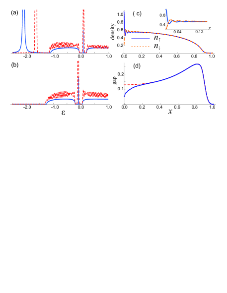
Figure 1: (a) Density of states for spin up atoms. (b) Density of states for spin down atoms. (c) Density profiles for both spin species. (d) Gap profile. In (a) and (b) solid and dashed lines represent results obtained using the $T$-matrix and BdG method, respectively. The dashed curve in (d) is the gap profile without the impurity. For all plots, $N_{\uparrow}=N_{\downarrow}=50$, and $u=-0.02E_{F}x_{TF}$, where $E_{F}$ is the Fermi energy and $x_{TF}=\sqrt{N}a_{{\rm ho}}$ is the Thomas-Fermi radius of the non-interacting system. The harmonic oscillator length and Thomas Fermi density at the origin are defined by $a_{{\rm ho}}=\sqrt{\hbar/(m\omega_{0})}$ and $n_{0}=2\sqrt{N}/(\pi a_{{\rm ho}})$. The dimensionless interaction parameter $\gamma=-mg/(\hbar^{2}n_{0})=1.25$. The units for density, energy and length are $n_{0}$, $E_{F}$ and $x_{TF}$, respectively.

To confirm that these results still hold when a trapping potential is present, as is always the case in the experiment, we add a harmonic potential $V_{T}=m\omega_{0}^{2}x^{2}/2$ to the system and diagonalize the Hamiltonian using the Bogoliubov-de Gennes (BdG) method de Gennes66 ; Hu07 ; BdG :

$$\left[\begin{array}[]{cc}H_{\uparrow}^{s}-\mu_{\uparrow}&-\Delta\\ -\Delta^{\ast}&-H_{\downarrow}^{s}+\mu_{\downarrow}\end{array}\right]\left[\begin{array}[]{c}u_{\eta}\\ v_{\eta}\end{array}\right]=E_{\eta}\left[\begin{array}[]{c}u_{\eta}\\ v_{\eta}\end{array}\right]\,,$$ (13)

where $H_{\sigma}^{s}=-(\hbar^{2}/2m)d^{2}/dx^{2}+V_{T}+U_{\sigma}+gn_{\bar{\sigma}}$, $n_{\uparrow}=\sum_{\eta}|u_{\eta}|^{2}\Theta(-E_{\eta})$, $n_{\downarrow}=\sum_{\eta}|v_{\eta}|^{2}\Theta(E_{\eta})$ and $\Delta=-g\sum_{\eta}u_{\eta}v_{\eta}^{*}\Theta(-E_{\eta})$, with $\Theta(\cdot)$ being the unit step function. The BdG equations above are solved self-consistently using a hybrid method whose details can be found in Ref. Hu07 . Once the solutions are found, we can calculate the LDOS at any points in space as $\rho_{\uparrow}(\epsilon)=\sum_{\eta}|u_{\eta}|^{2}\delta(\epsilon-E_{\eta})$ and $\rho_{\downarrow}(\epsilon)=\sum_{\eta}|v_{\eta}|^{2}\delta(\epsilon+E_{\eta})$. In practice, the $\delta$-function in the expression of the LDOS is replaced by a Gaussian with a small width of 0.02 $E_{F}$.

The dashed line in Fig. 1(a),(b) represents the LDOS at the magnetic impurity site ($x=0$) calculated using the BdG method. The agreement with the $T$-matrix method is satisfactory. The remaining discrepancies such as in the position of the resonant state below Fermi sea can be understood by considering that the $T$-matrix method neglects the trapping potential and is not fully self-consistent: the values of the chemical potentials, densities and pairing gap used in the $T$-matrix calculation are taken to be those from the BdG result in the absence of the impurity. The density and gap profiles of the trapped system are illustrated in Fig. 1(c),(d). Friedel oscillations with a spatial frequency close to $2k_{F}$ can be seen in the density profiles near the impurity. The magnetic impurity tends to break Cooper pairs, leading to a reduced gap size near the impurity as can be seen from Fig. 1(d).

Detection of the mid-gap state — As we have seen above, the mid-gap bound state induced by a magnetic impurity manifests itself in the LDOS. In general the LDOS provides valuable information on the quantum system and it is highly desirable to measure it directly. Great dividends have been reaped in the study of high $T_{c}$ superconductors where the scanning tunneling microscope (STM), which measures the differential current proportional to the LDOS, provides this functionSTM . In ultra-cold Fermi gases, radio-frequency (RF) spectroscopy Regal03 ; Gupta03 ; Grimm04 could serve as an analogous tool. The RF field induces single-particle excitations by coupling one of the spin species (say $|\uparrow\rangle$ atoms) out of the pairing state to a third state $|3\rangle$ which is initially unoccupied. In the experiment, the RF signal is defined as the average rate change of the population in state $|\uparrow\rangle$ (or state $|3\rangle$) during the RF pulse. The first generation RF had low resolution and provided averaged currents over the whole atomic cloud, which complicated interpretation of the signal due to the inhomogeneity of the sample stoof . More recently spatially resolved RF spectroscopy which provides local information has been demonstrated Ketterle07 . Here we show that a modified implementation of the spatially resolved RF spectroscopy can yield direct information of the LDOS and hence can serve as a powerful tool in the study of quantum gases.

To study the effect of the RF field, we make two additions to the total Hamiltonian (1):

$$H_{3} = \int dx\,\psi_{3}^{{\dagger}}(x)\left[-\frac{\hbar^{2}}{2m}\frac{d^{2}}{dx^{2}}+V_{3}(x)-\nu-\mu_{3}\right]\psi_{3}(x),$$

$$H_{T} = \int dx\,[T\psi_{3}^{{\dagger}}(x)\psi_{\uparrow}(x)+T\psi_{\uparrow}^{{\dagger}}(x)\psi_{3}(x)],$$

where $H_{3}$ represents the single-particle Hamiltonian of the state 3 (we assume that atoms in state 3 do not interact with other atoms), with $V_{3}$ being the trapping potential of the state and $\nu$ the detuning of the RF field from the atomic transition, $H_{T}$ represents the coupling between state 3 and spin-up atoms. Since RF photon wavelength is much larger than typical size of the atomic cloud, the coupling strength $T$ can be regarded as a spatially invariant constant. For weak RF coupling, one may use the linear response theory torma00 ; torma04 ; levin05 to obtain the RF signal which is proportional to $I(x)=\frac{d}{dt}\langle\psi_{3}^{{\dagger}}(x)\psi_{3}(x)\rangle$. Under the linear response theory, we have

$$I(x)\propto\int dx^{\prime}d\omega A_{\uparrow}(x,x^{\prime};\omega)A_{3}(x^{\prime},x,\omega+\mu_{\uparrow}-\mu_{3})f(\omega)\,,$$

where $f(\omega)$ is the Fermi distribution function which reduces to the step function at zero temperature, $A_{\alpha}$ is the spectral function for state $\alpha$. As state 3 is non-interacting, we have $A_{3}={\sum_{n}}\phi_{n}(x)\phi_{n}^{\ast}(x^{\prime})\delta(\omega+\mu_{\uparrow}+\nu-\epsilon_{n})$, where $\phi_{n}$ and $\epsilon_{n}$ are the single-particle eigenfunctions and eigen-energies of state 3, respectively. The key step in our proposal is that in the case where $V_{3}$ represents an optical lattice potential in the tight-binding limit, the dispersion of state 3 is proportional to the hopping constant $t$ which decreases exponentially as the lattice strength is increased. For sufficiently large lattice strength, we may therefore neglect the dispersion of state 3 since the lowest band is nearly flat. In other words, under such conditions, $\epsilon_{n}=\epsilon$ becomes an $n$-independent constant. Consequently $A_{3}(x,x^{\prime})\sim\delta(x-x^{\prime})$. In this limit and at zero temperature, the RF signal is then is directly related to the LDOS as:

$$I(x)\propto\rho_{\uparrow}(x,-\mu_{\uparrow}-\nu+\epsilon)\Theta(\mu_{\uparrow}+\nu-\epsilon)\,.$$ (14)

and the spatially resolved RF spectroscopy becomes a direct analog of the STM. A crucial point here is that only state 3 experiences the lattice potential. We note here that a spin-dependent optical lattice selectively affecting only one spin state has recently been realized in the lab of de Marco marco . The same technique can also be used to create magnetic impurity potentials by external light field.

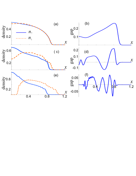
Figure 2: (Color online) Density (left panel) and gap (right panel) profiles of a trapped system under an extended Gaussian magnetic impurity potential. The width of the impurity potential is $a=0.2x_{TF}$, while the strength is $u=-0.12E_{F}x_{TF}$ for (a) and (b); $u=-0.4E_{F}x_{TF}$ for (c) and (d), and $u=-1.0E_{F}x_{TF}$ for (e) and (f). Other parameters and units are the same as in Fig. 1.

Extended impurity — Now we turn to Gaussian impurity potentials with finite width $U_{\sigma}(x)=u_{\sigma}e^{-x^{2}/a^{2}}/(a\sqrt{\pi})$. Since we obtain all of the previous (delta function) physics for narrow widths, we focus on relatively wide potentials. Examples of the density and gap profiles obtained from our BdG calculations are shown in Fig. 2. For an extended impurity potential of sufficient width, the Friedel oscillations are suppressed. Under appropriate conditions, the gap profiles exhibit FFLO-like oscillations FFLO , which has recently received considerable attention in studies of ultra-cold atoms randy ; Orso ; Demler . In previous experiments, polarized Fermi gas have been realized by preparing the gas with an overall population imbalance. Here the magnetic impurity breaks the local population balance and by tailoring the strength and/or the width of the magnetic impurity, one is able to control the magnitude of the population imbalance as shown in Fig. 2 which in turn controls the nature of the induced FFLO state. The impurity therefore provides us with a controlled way to create FFLO state.

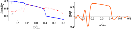
Figure 3: (Color online) Density (upper panel, in units of $(2E_{F})^{3/2}/(6\pi^{2})$) and gap (lower panel, in units of $E_{F}$) profiles along the $x$-axis of a 3D trapped system under an extended magnetic impurity potential. The impurity potential is uniform along the radial direction and has a Gaussian form with width $a=0.3x_{TF}$ along the $x$-axis. The strength of the impurity is $u=-0.07E_{F}x_{TF}$. The atom-atom interaction is characterized by the 3D scattering length $a_{s}$. Here we have used $1/(k_{F}a_{s})=-0.69$.

For simplicity, we have thus far focused on 1D systems. However, we have verified that the essential physics is also valid in higher dimensions. As an example, we illustrate in Fig. 3 the effect of an extended magnetic impurity in a 3D trapped system obtained by solving the BdG equations BdG . Here a total of 1100 atoms are trapped in an elongated cylindrical trapping potential $V(r,x)=\frac{m}{2}(\omega_{\bot}^{2}r^{2}+\omega_{x}^{2}x^{2})$ with trap aspect ratio $\omega_{\bot}/\omega_{x}=50$. The magnetic impurity centered at the origin, is radially uniform and has a Gaussian profile along the axial direction ($x$-axis). From the density and gap profiles shown in Fig. 3, one can easily identify the induced FFLO regions both near the center and the edge of the trap. In particular, the density oscillations in the spin-down component near trap center may be used as a signature of the FFLO state.

In conclusion, we have investigated the effects of a single classical magnetic impurity on a neutral fermionic superfluid. We show that a magnetic impurity can be used to manipulate novel quantum states in a Fermi gas. For example, it will induce a mid-gap bound state inside the pairing gap for both spin species. We have proposed an STM-like scheme based on the modified spatially resolved RF spectroscopy to measure the local density of states, from which the mid-gap bound states can be unambiguously detected. As different quantum phases of cold atoms will manifest thems‘elves in their distinct LDOS, we expect this method will find important applications beyond what is proposed here and become an invaluable tool in the study of quantum gases. Finally, by considering an extended impurity potential in both 1D and 3D systems, we demonstrate the realization of the still unobserved FFLO phase in a controlled manner.

Interesting future directions could involve the study of periodic or random arrays of localized impurities which may be exploited to induce novel quantum states in Fermi superfluids and the consideration of a quantum impurity with its own internal degrees of freedom. Such a system may allow us to explore Kondo physics in cold atoms.

This work is supported by the NSF, the Welch Foundation (Grant No. C-1669) and by a grant from the Army Research Office with funding from the DARPA OLE Program. HH acknowledges the support from an ARC Discovery Project (Grant No. DP0984522). Y.C. was supported by the NSFC and the State Key Programs of China. We would like to thank Qiang Han for useful discussions.

References

- (1) A. V. Balatsky, I. Vekhter, and J.-X. Zhu, Rev. Mod. Phys. 78, 373 (2006).
- (2) H. Alloul et al., Rev. Mod. Phys. 81, 45 (2009).
- (3) A.P. Mackenzie et al., Phys. Rev. Lett. 80, 161 (1998).
- (4) P. T. Sprunger et al., Science 275, 1764 (1997).
- (5) A. J. Millis, Solid State Commun. 126, 3 (2003).
- (6) G. Modugno, Rep. Prog. Phys. 73, 102401 (2010).
- (7) C. Zipkes et al., Nature 464, 388 (2010).
- (8) K. Targońska and K. Sacha, Phys. Rev. A 82, 033601 (2010); E. Vernier et al., Phys. Rev. A 83, 033619 (2011).
- (9) I. Bausmerth et al., Phys. Rev. A 79, 043622 (2009).
- (10) P. J. Hirschfeld, D. Vollhard, and P. Wölfle, Solid State Commun. 59, 111 (1986).
- (11) L. Yu, Acta Phys. Sin. 21, 75 (1965); H. Shiba, Prog. Theor. Phys. 40, 435 (1968); A. I. Rusinov, Sov. Phys. JETP 29, 1101 (1969).
- (12) P. de Gennes, Superconductivity of Metals and Alloys (Addison-Wesley, New York, 1966).
- (13) X.-J. Liu, H. Hu, and P. D. Drummond, Phys. Rev. A 75, 023614 (2007); X.-J. Liu, H. Hu, and P. D. Drummond, Phys. Rev. A 76, 043605 (2007).
- (14) L. O. Baksmaty et al.,Phys. Rev. A 83, 023604 (2011).
- (15) Ø. Fischer et al., Rev. Mod. Phys. 79, 353 (2007).
- (16) C. A. Regal and D. S. Jin, Phys. Rev. Lett. 90, 230404 (2003).
- (17) S. Gupta et al., Science 300, 1723 (2003).
- (18) C. Chin et al., Science 305 1128 (2004).
- (19) P. Massignan, G. M. Bruun, and H. T. C. Stoof, Phys. Rev. A 77 031601(R) (2008).
- (20) Y. Shin et al., Phys. Rev. Lett 99 090403 (2007).
- (21) P. Törmä and P. Zoller, Phys. Rev. Lett. 85, 487 (2000); G. M. Bruun et al., Phys. Rev. A 64, 033609 (2001).
- (22) J. Kinnunen, M. Rodriguez, and P. Törmä, Science 305, 1131 (2004); Phys. Rev. Lett. 92, 230403 (2004).
- (23) Y. He, Q. Chen, and K. Levin, Phys. Rev. A 72, 011602(R) (2005); Y. He et al., Phys. Rev. A 77, 011602(R) (2008).
- (24) D. McKay and B. DeMarco, New J. Phys. 12 055013 (2010).
- (25) P. Fulde and R. A. Ferrell, Phys. Rev. 135 A550 (1964); A. I. Larkin and Y. N. Ovchinnikov Sov. Phys.-JETP 20 762 (1965).
- (26) Y.-A. Liao et al., Nature 467, 567 (2010).
- (27) G. Orso, Phys. Rev. Lett. 98, 070402 (2007); H. Hu, X.-J. Liu, and P. D. Drummond, Phys. Rev. Lett. 98, 070403 (2007).
- (28) I. Zapata et al., Phys. Rev. Lett. 105, 095301 (2010); K. Sun et al., Phys. Rev. A 83, 033608 (2011).