Approximate magnifying perfect lens with positive refraction

Abstract

We propose a device with a positive isotropic refractive index that creates an approximate magnified perfect real image of an optically homogeneous three-dimensional region of space within geometrical optics. Its key ingredient is a new refractive index profile that can work as an approximate perfect lens on its own, having a very moderate index range.

In perfect imaging, light rays emerging from any point P of some three-dimensional region are perfectly (stigmatically) reassembled at another point P’, the image of P. Perfect imaging has been one of the hot topics in modern optics since 2000 when J. Pendry showed that a slab of a material with negative refractive index Pendry2000 can work as a perfect imaging device (perfect lens). Much effort has then been put into designing and constructing perfect lenses based on materials with negative refractive index Shalaev2007-review , which led e.g. to demonstrations of sub-wavelength resolution Fang2005-neg_n-silver_imaging .

On the other hand, as early as in 1854 J. C. Maxwell found a device with an isotropic and positive refractive index that images the whole space perfectly, which he called fish eye. More than 150 years later, U. Leonhardt and T. Philbin showed that Maxwell’s fish eye provides perfect imaging not only in terms of geometrical optics also in the full framework of wave optics Ulf2009-fisheye ; Ulf2010-fisheye , and therefore enables sub-wavelength resolution similarly as perfect lenses based on negative refraction. Recent experiments have confirmed this Ma2010-fisheye . Only a few other perfect lenses with an isotropic positive refractive index were known until recently. Even less was known about devices that would image perfectly homogeneous regions of space, i.e., regions with a uniform refractive index. Indeed, even in the last issue of Born and Wolf’s Principles of Optics BornWolf we read that the only known example of such a device is a plane mirror or a combination thereof. This has been changed by a recent excellent work of J. C. Miñano Minano2006 who proposed several new perfect lenses imaging homogeneous regions and also showed that some well-known optical devices such as Eaton lens or Luneburg lens Luneburg1964 are in fact perfect lenses as well. All of them have unit magnification, giving an image of the same size as the original object.

Here we present a lens that provides an approximate perfect real image of a homogeneous region of 3D space with an arbitrary magnification. Our device is a non-trivial combination of Maxwell’s fish eye and a new refractive index profile. This profile equipped with a spherical mirror can work as an approximate perfect lens on its own, giving a real image of a homogeneous sphere and using just a moderate refractive index range. Our lens employs isotropic material with positive refractive index.

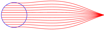
Figure 1: Medium with a spherically-symmetric refractive index that focuses parallel rays inside an optically homogeneous unit sphere (blue) to a point at distance $R$ from its center (here $R=7$).

The key ingredient of our lens is a spherically symmetric refractive index profile $n(r)$ that focuses all parallel rays within a sphere of, say, radius 1 and a constant refractive index to a point at a distance $R>1$ from the center of the sphere (Fig. 1). To see why this can be useful, imagine that a spherical mirror is placed at the radius $R$ (Fig. 2). A ray that emerges from a point P inside the unit sphere reaches the mirror, is reflected and enters the sphere again. Because of the law of reflection and the above focusing property, the ray after re-entering the sphere will be parallel with the original ray and lie opposite to it from the center of the sphere. Therefore it will pass approximately through the point P’ that is opposite of P, viewed from the center of the sphere. This shows that an approximate perfect real image of point P is formed at point P’.

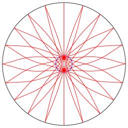
Figure 2: Approximate perfect lens formed by surrounding the medium from Fig. 1 with a spherical mirror of radius $R$ (shown in black).

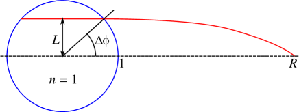
Figure 3: Notation used for deriving the refractive index profile $n_{R}(r)$.

To find the corresponding refractive index $n(r)$, we use the expression for the polar angle swept by the ray during propagation from $r=1$ to $r=R$ Landau-shorter (see Fig. 3):

$$\Delta\phi=L\int_{1}^{R}\frac{{\rm d}r}{r\sqrt{n^{2}r^{2}-L^{2}}}.$$ (1)

Here $L=nr\sin\alpha$ and $\alpha$ denotes the angle between the ray and the radius vector. $L$ corresponds to the angular momentum in the equivalent mechanical problem Ulf-Thomas-book and is conserved in any spherically-symmetric refractive index profile. Assuming that the refractive index inside the unit sphere is equal to one, $L$ is equal to the distance of the ray from the center and $\Delta\phi=\arcsin L$ (Fig. 3). Inserting this into Eq. (1) and making the substitutions $r={\rm e}^{x}$, $N=nr$, we obtain an integral equation

$$L\int_{0}^{X}\frac{\mathrm{d}x}{\sqrt{N(x)^{2}-L^{2}}}=\arcsin{L},$$ (2)

where $X=\ln R$. As has been shown NJP , this equation does not have an exact solution; we therefore employed two different methods to find an approximate solution $N(x)$ numerically.

In the first method, we changed the integration variable in Eq. (2) from $x$ to $N$ to obtain

$$L\int^{N_{1}}_{1}u(N)\frac{\mathrm{d}N}{\sqrt{N^{2}-L^{2}}}=\arcsin{L},$$ (3)

where $u(N)={\rm d}x/{\rm d}N$ and $N_{1}=Rn(R)$. This equation can be solved by Galerkin’s method for the linear integral equations of the first kind Polyanin as follows. The unknown function $u(N)$ is first expanded as $u(N)=\sum_{i}A_{i}\varphi_{i}(N)$, where $A_{i}$ are real coefficients and $\varphi_{i}(N)$ is a set of functions on the interval $(1,N_{1})$. Substituting this expression into Eq. (3) and interchanging the summation and integration, we obtain

$$\sum_{i}A_{i}g_{i}(L)=\arcsin{L}\,,$$ (4)

where $g_{i}(L)=L\int^{N_{1}}_{1}\varphi_{i}(N)(N^{2}-L^{2})^{-1/2}\,\mathrm{d}N$. For a chosen set of functions $\varphi_{i}(N)$ we need to calculate the unknown coefficients $A_{i}$. For this purpose we define another set of functions $\psi_{j}(L)$ on the interval $(0,1)$. Multiplying both sides of Eq. (4) by $\psi_{j}(L)$, integrating over $L$ from $0$ to $1$ and interchanging the order of summation and integration, we obtain the matrix equation

$$\sum_{i}\sigma_{ij}A_{i}=B_{j}\,,$$ (5)

where $\sigma_{ij}=\int^{1}_{0}\psi_{j}(L)g_{i}(L)\,\mathrm{d}L$ and $B_{j}=\int^{1}_{0}\psi_{j}(L)\arcsin{L}\,\mathrm{d}L$. The unknown coefficients $A_{i}$ are then solutions of the system of linear equations (5). Using the calculated coefficients $A_{i}$, the approximate solution of function $u(N)$ is finally obtained. In our calculation, we have chosen polynomials as basis functions, $\varphi_{i}(N)=N^{i},\psi_{j}(L)=L^{j}$, with $i,j$ running from $0$ to some maximum value $M$.

The second, less sophisticated but equally efficient method, was based on numerical minimization of the lens aberration. We have represented the function $N(x)$ in Eq. (2) by a polynomial $N(x)=1+\sum_{1}^{k}a_{i}x^{i}$ with coefficients $a_{i}$ and calculated the aberration

$$A=\sum_{\{L_{i}\}}\left(L_{i}\int_{0}^{X}\frac{\mathrm{d}x}{\sqrt{N(x)^{2}-L_{i}^{2}}}-\arcsin{L_{i}}\right)^{2}$$ (6)

as a function of $a_{1},\dots,a_{k}$. Here $L_{i}$ denotes a chosen set of representative values of $L$ from the interval $(0,1]$. To find the minimum aberration, we have employed the numerical function NMinimize of the program Mathematica. It turned out that using polynomial of degree $k=5$ and ten uniformly distributed values of $L_{i}$ gave a refractive index with a negligible aberration; for example, for $X=3$ the mean difference of the angle $\Delta\phi$ from the correct value was $10^{-6}$ radians. It turned out that the method works very well for $X\geq 2$, but does not work for $X\leq 1$, which would correspond to $R\leq\rm e$.

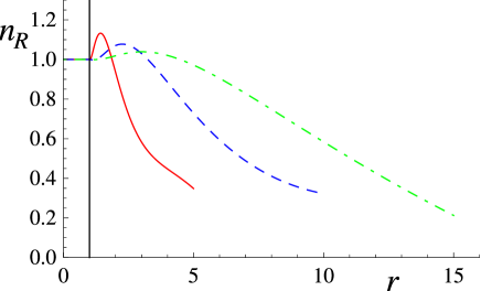
Figure 4: Refractive index $n_{R}(r)$ calculated by the method of minimizing aberration for $R=5$ (red full line), $R=10$ (blue dashed line) and $R=15$ (green dash-dotted line). The vertical line marks the border of the homogeneous region at $r=1$.

Both methods give similar results for $n(r)$. Fig. 4 shows the refractive index $n(r)$ obtained by the second method for several values of $R$. The ray trajectories are shown in Fig. 1 for $R=7$. Of course, the whole function $n(r)$ (including the region $r<1$) can be multiplied by any real constant $C$ without changing the focusing properties of the lens. In addition, the size of the lens can be scaled by an arbitrary factor $D$. If we denote the original refractive index distribution by $n_{R}(r)$ instead of $n(r)$ to emphasize that it depends on the parameter $R$, then the most general refractive index of our lens becomes $n(r)=Cn_{R}(r/D)$. This lens focuses parallel rays within the sphere of radius $D$ to the point at the distance $DR$ from its center. Using for instance $R=7$ and setting $C=2.74$ to bring $n(r)$ above one in the whole lens, we get $1\leq n\leq 3.11$, which is a very moderate range.

Having described the lens that approximately focuses parallel rays to a single point, we proceed now to construction of the magnifying lens. For this purpose, we divide the whole Euclidean 3D space into three regions denoted I, II and III (see Fig. 5). Using spherical coordinates $(r,\theta,\phi)$ centered at a point O, we define the regions as follows. Region I is given by the conditions $0\leq r\leq R$ and $0\leq\theta<\pi/2$; region II is given by the conditions $0\leq r\leq mR$ and $\pi/2<\theta\leq\pi$, where $m\geq 1$ is going to be the lens magnification; region III occupies the rest of the space.

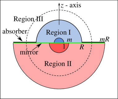
Figure 5: Regions in the approximate magnifying perfect lens, the $z$ axis ($\theta=0$) being vertical. The radii of the individual spheres are marked along horizontal axis. The dashed line shows the radius $a=R\sqrt{m}$ of Maxwell’s fish eye profile located in Region III. The object and image spaces are marked by a slightly darker color.

Refractive index in region I is given by the above described profile, i.e., $n_{\rm I}=n_{R}(r)$. Refractive index in region II is $n_{\rm II}=n_{R}(r/m)/m$. Refractive index in region III is described by Maxwell’s fish eye profile

$$n_{\rm III}=\frac{n_{1}(1+1/m)}{1+r^{2}/(mR^{2})},$$ (7)

with the fish eye radius, i.e., the radius of ray that runs at a fixed distance from the center O, equal to $a=R\sqrt{m}$, and $n_{1}=n_{R}(R)$. It is easy to check that the refractive index is continuous at the hemispherical interfaces of region III with both regions I and II, i.e., $n_{\rm I}(R)=n_{\rm III}(R)$ and $n_{\rm II}(mR)=n_{\rm III}(mR)$.

The radius $a$ of Maxwell’s fish eye was chosen such that it images the hemispheric interface of regions I and III to the hemispheric interface of regions II and III. Indeed, the relation of radial coordinates $r,r^{\prime}$ of a point and its image in the fish eye is $rr^{\prime}=a^{2}$ BornWolf , which is satisfied in our case.

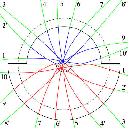
Figure 6: Ray tracing in the approximate magnifying perfect lens with $m=3/2$. The parts of the rays in regions I, II and III are shown in blue, red and green, respectively. The numbers help to match the two parts of the same ray. The primes mark the rays that are reflected from the mirror before entering region III while unprimed rays are reflected after leaving region III.

We will show now that this device approximately images the object space, which is the homogeneous hemisphere of radius $r=1$ and refractive index $n=1$ in region I, to the image space, which is the homogeneous hemisphere with radius $r=m$ and refractive index $n=1/m$ in region II (see Fig. 5). Consider a ray emerging from some point P placed at the radius vector $\boldsymbol{r}_{\rm P}$ in the object space in the direction described by a unit vector $\boldsymbol{\nu}$ that has a positive component in $z$-direction. Due to the focusing properties of the profile $n_{R}(r)$ in region I, it will hit the interface of regions I and III at the point A$\,=R\boldsymbol{\nu}$. The Maxwell’s fish eye profile in region III will ensure that the ray will then propagate along a circle and hit the interface of regions III and II at the point B$\,=-mR\boldsymbol{\nu}$. Moreover, since the ray is a segment of a circle, clearly the angle between the ray and the straight line AOB at point A is the same as the angle between the ray and the line AOB at point B. The ray hence enters region II with the same impact angle with which it left region I. Now since the index profiles in regions I and II differ only by a spatial scaling by $m$ and a multiplicative factor, it is clear that the shape of the ray in region II will be the same as its shape in region I, up to scaling by $m$. In particular, when the ray enters the image space, it will resume its original propagation direction $\boldsymbol{\nu}$, but the straight line on which it lies will be $m\times$ more distant from the origin O than the straight line of the first segment of the ray in region I. This means that the ray will be directed towards the point P’ placed at $m\boldsymbol{r}_{\rm P}$. Now if many rays emerge from point P, they will form an image at P’; however, this point lies outside of region II, so the image would be virtual. Because of this, we place a mirror at the interface of regions I and II that changes the virtual image at P’ into a real image at a point P” at position $\hat{Z}m\boldsymbol{r}_{\rm P}$, with $\hat{Z}$ meaning the operation of inverting the $z$-coordinate. Furthermore, if we make the mirror double-sided, then we can take advantage also of the rays that emerge “down” from P (those with negative $z$-component of $\boldsymbol{\nu}$). These rays will be reflected from the mirror while still propagating in object space and then reach the image P” without a further reflection, as marked in Fig. 6 by primes. It turns out, however, that some rays with positive $z$-component of $\boldsymbol{\nu}$ will hit the flat interface between regions III and II. Since it is not possible to use these rays for imaging, we block them by placing an absorber at this flat interface on the side of region III, keeping the mirror on the side of region II. This way, not all rays emerging from P reach P”, but it is a negligible minority of rays that are lost in this way, especially if the magnification $m$ is not too large. Still, it is not necessary for a device to capture all rays to be called a perfect lens within geometrical optics BornWolf .

In summary, we have proposed a lens that makes an approximate magnified perfect real image of a homogeneous 3D region. Performance of this lens in the full wave optics regime is a subject of investigation, but we believe that it may provide sub-wavelength resolution similarly as Maxwell’s fish eye. Manufacturing this lens would be difficult because the refractive index of Maxwell’s fish eye profile in region III goes to zero for $r\to\infty$, and rays forming the image do get very far from the origin. Multiplying the whole index profile by a large number will not help much because then the index in the object and the image spaces then becomes very large. An option how to reduce refractive index range significantly would be to position regions I and II differently and use some other, not spherically symmetric index profile in region III to image the surface of one sphere to the other. On the other hand, the index profile $n_{R}(r)$ that is a part of the device can work as an approximate perfect lens on its own, requiring just a moderate refractive index range and therefore having potential to become a practical device.

After we published this paper on the arXiv, our colleague Klaus Bering proved analytically that there exists no function $N(x)$ that solves the integral equation (2) exactly and therefore the refractive index $n_{R}$ with the focusing properties does not exist either. Before that, we believed that Eq. (2) does have an exact solution but that we just could not find it. A detailed proof of the non-existence of the solution is given in Ref. NJP . In spite of that, we believe that even though our device works only approximately, it still may have value for further research; therefore we have replaced the paper on arXiv instead of withdrawing it. In the meantime, we have found another method for designing magnifying perfect lenses (or absolute instruments) PRA that works exactly and is much more flexible than the method presented in this paper.

We thank Klaus Bering, Ulf Leonhardt, Michael Krbek and Aaron Danner for very useful discussions.

References

- (1) J. B. Pendry, Phys. Rev. Lett. 85, 3966 (2000).
- (2) V. M. Shalaev, Nature Photonics 1, 41 (2007).
- (3) N. Fang, H. Lee, C. Sun, and X. Zhang, Science 308, 534 (2005).
- (4) U. Leonhardt and T. G. Philbin, Phys. Rev. A 81, 011804(R) (2010).
- (5) U. Leonhardt, New J. Phys. 11, 093040 (2009).
- (6) Y. G. Ma, C. Ong, S. Sahebdivan, T. Tyc, and U. Leonhardt (2010), eprint arXiv:1007.2530.
- (7) M. Born and E. Wolf, Principles of optics (Cambridge University Press, 2006).
- (8) J. C. Miñano, Opt. Express 14, 9627 (2006).
- (9) R. K. Luneburg, Mathematical Theory of Optics (University of California Press, Berkeley, 1964).
- (10) L. D. Landau and E. M. Lifshitz, A shorter course of theoretical physics (Pergamon Press, 1972).
- (11) U. Leonhardt and T. Philbin, Geometry and Light: The Science of Invisibility (Dover, Mineola, 2010).
- (12) T. Tyc, L. Herzánová, Martin Šarbort and Klaus Bering, New J. Phys. 13, 115004 (2011).
- (13) A. Polyanin and A. Manzhirov, Handbook of integral equations (Chapman & Hall, 2008).
- (14) T. Tyc, Phys. Rev. A 84, 031801(R) (2011).