A model of Mira’s cometary head/tail entering the Local Bubble

Abstract

We model the cometary structure around Mira as the interaction of an AGB wind from Mira A, and a streaming environment. Our simulations introduce the following new element: we assume that after ${200~{}\mathrm{kyr}}$ of evolution in a dense environment Mira entered the Local Bubble (low density coronal gas). As Mira enters the bubble, the head of the comet expands quite rapidly, while the tail remains well collimated for a ${>100~{}\mathrm{kyr}}$ timescale. The result is a broad-head/narrow-tail structure that resembles the observed morphology of Mira’s comet. The simulations were carried out with our new adaptive grid code Walicxe, which is described in detail.

1. Introduction

Mira is a well studied binary system. Mira A is a prototypical, thermally pulsating luminous AGB star (which in fact gives name to the so-called Mira class of variables), while Mira B is a much less luminous star, believed to be a white dwarf or a main sequence star. Recently, the discovery of a cometary structure of $\sim 2\arcdeg$ in the sky with its head centered on Mira, by Martin et al. (2007), with the GALEX satellite, has generated a renewed interest in this system. In order to compare the observations with our models we include in Figure 1 a schematic diagram of the UV image of Martin et al. (2007).

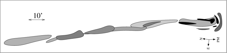
Figure 1.— Sketch of the UV image of the tail of Mira observed with GALEX, fig. 1a of Martin et al. (2007). The intensity is represented by the different shades of gray (darker corresponds to a higher intensity). The orientation (N,E) and proper motion (PM) are indicated by the arrows below the head of the comet.

The broad-band UV filters (FWHM $\Delta\lambda=256,~{}730\,$Å, centered at $\lambda_{c}=1516,~{}2267\,$Å) in GALEX make difficult to discriminate the physical mechanism responsible for the observed emission. Martin et al. (2007) suggested that most of the observed emission in the tail of Mira could be due to fluorescent $\mathrm{H_{2}}$ lines, while in regions closer to the bow-shock it is likely that other species, such as C IV could contribute to the emission.

The distance to Mira, estimated from Hipparcos is $107~{}\mathrm{pc}$ (Knapp et al., 2003). The system Mira moves at a high speed ($\sim 125~{}\mathrm{km~{}s^{-1}}$) with respect to its surrounding medium, as deduced from its proper motion (Turon et al., 1993) and radial velocity (Evans, 1967). The physical size of the cometary tail, assuming the Hipparcos distance is $\sim 4\mathrm{pc}$.

New observations and/or reexamination of previous observations have been made in several wavelenghts, including H I 21cm (Matthews et al., 2008), IR (Ueta, 2008), and optical (Meaburn et al., 2009). Recent theoretical work has been done by Wareing et al. (2007); Raga et al. (2008); Raga & Cantó (2008). Wareing et al. (2007) performed a 3D hydrodynamical simulation of the interaction between an isotropic AGB wind and the ISM, modeled as a plane-parallel wind (considering a reference system in which Mira is at rest). Raga et al. (2008) included an inhomogeneous AGB wind, resulting in a more complicated shock structure for the cometary head (possibly more consistent with the observations). These two models, however, have one flagrant flaw: if the models are adjusted to produce the correct size for the cometary head, the tail that they produce is significantly broader than the one of Mira’s comet.

The reason for this discrepancy with the observations lies in the fact that the ISM density in those models is estimated by assuming ram pressure balance between Mira’s wind and the ISM at the tip of the head of the cometary structure. Therefore, the distance between the front of the bow-shock and Mira is consistent with the observations. However, the tail produced by the model has a width comparable to the head, while Mira’s comet shows a considerably narrower tail (see Fig 1).

Wareing et al. (2007) speculated that Mira could have recently crossed into the Local Bubble (a tenuous region of coronal gas). Most of the tail could then have formed outside the Local Bubble, in a higher density ISM, resulting in the observed, narrow tail structure. In the present paper, we explore this possibility through a set of axisymmetric numerical simulations of a travelling star+wind system which emerges into a hot, coronal gas bubble.

The paper is organized as follows: in section 2 we describe the model, including a review of the analytical solution of the wind/streaming environment by Wilkin (1996) and Cantó et al. (1996). The setup of the numerical simulations is presented in section 3, followed by the results in section 4, and a summary in section 5. As this paper is the first publication with our new hydrodynamical code Walicxe, we include an appendix describing the code in detail, as well as some tests.

2. The model

Following Wareing et al. (2007) and Raga et al. (2008) we model Mira’s cometary tail as the interaction of a slow, dense, wind that arises from the AGB star Mira A, with a fast, lower-density, plane-parallel wind that results from the motion of Mira through the ISM (the simulations are performed in the reference frame in which Mira is at rest), as shown in the schematic diagram of Figure 2.

Figure 2.— Schematic of the two-wind interaction model. The interaction of a moving spherical wind source (Mira A) and its surrounding ISM can be modeled, in a reference frame with Mira A at rest, as a stationary wind source accompanied by a streaming ISM. In this figure, we also illustrate the spherical radius $R$ used in the analytical model, the polar angle $\theta$, and the standoff distance $R_{\mathrm{s}}$.

The structure that results from the interaction between a streaming, plane-parallel flow and a spherical wind has a cometary shape that has been described analytically, considering conservation of linear and angular momentum in a “thin-shell” approximation (Wilkin, 1996; Cantó et al., 1996). With this formalism, the shape of bow-shock is found to have the form:

$$R(\theta)=R_{\mathrm{s}}\csc\theta\sqrt{3(1-\theta\cot\theta)},$$ (1)

where $R$ is the spherical radius (measured from the center of the isotropic wind source), $\theta$ is the polar angle (measured from the symmetry axis, aligned with the direction towards the impinging, plane-parallel flow), and $R_{\mathrm{s}}$ is the stagnation radius (or standoff distance, see Figure 2). The stagnation radius (point of closest approach to the spherical wind source) is given by the ram-pressure balance between the two winds:

$$\frac{\dot{M}_{\mathrm{w}}v_{\mathrm{w}}}{4\pi R_{\mathrm{s}}^{2}}=\rho_{\mathrm{a}}v_{\mathrm{a}}^{2},$$ (2)

where $\dot{M}_{\mathrm{w}}$ is the mass loss rate of Mira, $v_{\mathrm{w}}$ its terminal wind velocity, $\rho_{\mathrm{a}}$ the ambient (ISM) mass density, and $v_{\mathrm{a}}$ the velocity of the star moving through the surrounding environment.

Figure 3.— Analytical solution of the two-wind “thin-shell” model (Wilkin, 1996; Cantó et al., 1996) for three different stagnation radii: ${R_{\mathrm{s}}=0.1,~{}0.5,1.0}$ (solid, dotted and dashed lines, respectively). The position of the spherical wind source is at $(0,0)$, marked by the star. The plane-parallel wind impinges form the right as in Fig. 2.

Figure 3 shows the locus of the interaction region (location of the thin-shell, and shape of the bow-shock structure) for different stagnation radii. Notice that for smaller $R_{\mathrm{s}}$ the cometary tail becomes narrower.

3. The numerical setup

We performed two hydrodynamical simulations of Mira’s tail with the new code Walicxe. The code solves the gas-dynamic equations in a block based adaptive mesh that is designed to run in parallel on machines with distributed memory (i.e. clusters).

Walicxe can be run with a Cartesian two-dimensional mesh, or an axisymmetric (cylindrical) grid. For this particular problem we have used the axisymmetric version of the code with the hybrid HLL-HLLC Riemann solver (see the Appendix for details).

Along with the gas-dynamic equations, a rate equation for hydrogen is solved. The resulting H ionization fraction is used to compute the radiative energy losses, which are obtained with the parametrized cooling function (that depends on the temperature, density and hydrogen ionization fraction) described in Raga & Reipurth (2004).

The simulations have 5 root blocks of $16\times 16$ cells each, aligned along the axial direction ($z-$axis). We allow $7$ levels of refinement, yielding an equivalent resolution of $1024\times 5120$ (radial$\times$axial) cells at the highest grid resolution. The computational domain extends $[(0,0.25)\times(0,1.25)]\times 10^{19}$ cm in the radial and axial directions, respectively. Thus, the resolution at the highest level of refinement is $\approx 2.4\times 10^{15}$ cm. We impose a reflective boundary condition along the symmetry axis ($r=0$). Open boundary conditions are used at $r=0.25\times 10^{19}~{}\mathrm{cm}$ and $z=0$.

In both models the spherical wind has the following properties. It is injected (at every timestep) in a spherical region of $3\times 10^{16}\mathrm{cm}$ radius, centered at $r=0$, $z=1.05\times 10^{19}~{}\mathrm{cm}$. The density inside the injection region follows an $\propto R^{-2}$ law ($R$ is the spherical radius measured from the position of the wind source), scaled so that the mass-loss rate is $\dot{M}_{\mathrm{w}}=3\times 10^{-7}~{}\mathrm{M_{\odot}yr^{-1}}$. The wind is neutral, has a temperature of $T_{\mathrm{w}}=10^{2}~{}\mathrm{K}$, and an outward, radially directed velocity $v_{\mathrm{w}}=5~{}\mathrm{km~{}s^{-1}}$. The values of the physical parameters of Mira’s wind were taken from the observational studies of CO lines by Young (1995) and Ryde et al. (2000).

At the initial time ($t=0$), both models are identical, with a plane-parallel wind that fills the computational domain (except inside the sphere in which the isotropic wind is imposed), which is replenished by an inflow condition at $z=1.25\times 10^{19}~{}\mathrm{cm}$. The ISM is homogeneous, with a hydrogen number density $n_{\mathrm{H}}=1~{}\mathrm{cm^{-3}}$ (consistent with the ISM in the galactic plane, just outside the Local Bubble in the vicinity of Mira, see Vergely et al. 2001), and a velocity $v_{\mathrm{a}}=125~{}\mathrm{km~{}s^{-1}}$ (in the $-z$ direction). The wind and ISM are neutral, except for a seed electron density assumed to arise from singly ionized C (i.e. the minimum ionization fraction is $10^{-4}$). The ISM has a temperature of $T_{\mathrm{a}}=10^{3}~{}K$.

In model M1, we evolve these initial/boundary conditions up to an integration time of $350~{}\mathrm{kyr}$. Model M1 corresponds to the evolution of Mira outside of the Local Bubble, in a uniform medium dense enough to produce the narrow tail as observed.

In model M2, we simulate Mira entering the Local Bubble, a region much hotter and tenuous than the average ISM. To achieve this, after $200~{}\mathrm{kyr}$ of evolution in the same medium as model M1, we raise the temperature of the ISM that enters the computational domain to $T_{\mathrm{a}}=10^{6}~{}K$, lower its density to $n_{\mathrm{H}}=5\times 10^{-2}~{}\mathrm{cm^{-3}}$ (from the observations by Lallement et al., 2003), and change its ionization fraction to $1$ (fully ionized hydrogen). We then let this configuration evolve up to a $t=350~{}\mathrm{kyr}$ integration time.

The model of Mira entering the Local Bubble is well justified by the current Galactic Position of Mira $(l,b)=(168,-58)$ (Perryman et al., 1997; Wareing et al., 2007). This position puts Mira inside, but close to the edge of the Local Bubble, as can be seen from the maps presented by Lallement et al. (2003). Given the high velocity of Mira, in the $\sim 300~{}\mathrm{kyr}$ that it takes to form a tail of $4~{}\mathrm{pc}$, it would have traveled approximately $38~{}\mathrm{pc}$. This distance is enough to place the starting point of the tail formation outside the Local Bubble.

4. Results

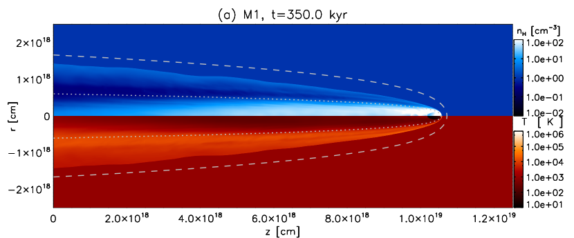
Figure 4.— Density (top half of each panel), and temperature (bottom half) stratifications at a $t=350~{}\mathrm{kyr}$ integration time, for the two models. The numerical values are shown in the logarithmic gray-scale (color-scale in the on-line version) bars at the right of each panel. We have included in both panels the analytical solution for the bow-shock for the two stagnation radii used (see text for details): the dotted line is for $R_{\mathrm{s}}=4.9\times 10^{16}~{}\mathrm{cm}$ and the dashed line for $R_{\mathrm{s}}=2.2\times 10^{17}~{}\mathrm{cm}$. The temperature panel has been reflected on the symmetry axis for visual purposes.

We let the models to evolve up to an integration time of $350~{}\mathrm{kyr}$, which is of the order of the time needed to form a cometary tail of $\sim 4~{}\mathrm{pc}$ in length (the size of the structure observed with GALEX). Figure 4 shows the density (top half of the panels) and temperature distributions (bottom half) of M1 and M2 at the final evolutionary stage.

From the top panel in Figure 4 we can see that after $350~{}\mathrm{kyr}$ a narrow tail, of axial and radial dimensions comparable with the observations of Mira, is formed. However, the stand-off distance (in agreement with the analytical prediction in eq. 2) is $R_{\mathrm{s}}\sim 4.9\times 10^{16}~{}\mathrm{cm}$, which is much closer to the source compared to the $R_{\mathrm{s}}\sim 3.1\times 10^{17}~{}\mathrm{cm}$ that can be deduced from the observations of Mira’s comet. The analytical solution for the parameters of model M1, plotted as a dotted line, traces well the region that separates the dense and cold material which arises from Mira’s wind, and the hotter, lower density shocked ISM. This can be seen more clearly in the following section, where we separate the contribution of the wind and show column density maps.

The bottom panel of Figure 4 shows the tail that would be produced if Mira entered the Local Bubble some $145~{}\mathrm{kyr}$ ago (i. e., model M2). The analytical solution for the parameters used for the Local Bubble is included as a dashed line. The corresponding standoff distance for model M2 is at $R_{\mathrm{s}}=2.2\times 10^{17}~{}\mathrm{cm}$ to the right of Mira, a distance that is close to what is observed ($3.1\times 10^{17}~{}\mathrm{cm}$).

This standoff distance, and the corresponding width of the tail (dashed line) are much larger than observations. However, the change from one stationary configuration to the other is not instantaneous. As the cometary flow expands after entering the Local Bubble the head grows rapidly. Approximately $20~{}\mathrm{kyr}$ after the entrance of Mira into the Local Bubble we obtain a structure that resembles remarkably well the broad-head/narrow-tail of Mira’s comet, such tail remains well collimated for at least $100~{}\mathrm{kyr}$. It is only after $150~{}\mathrm{kyr}$ of entering the Local Bubble that the tail becomes somewhat wider than the UV observations (see time sequence in the following section).

A clear difference in the wind/environment interface can be seen in models M1 and M2. In model M2, the outer boundary of the region filled by the stellar wind shows a more complex structure, which fragments the tail downstream from the wind source. Such structures are absent in Model M1 (see Figure 4). This difference is a result of the fact that while the wind/environment boundary has a highly supersonic velocity shear in model M1, this shear is barely transonic in model M2 (as Mira’s motion is basically sonic with respect to the hot, Local Bubble environment). It is a well known experimental result that the spreading rate of sonic mixing layers is much larger than the one of high Mach number mixing layers (see Cantó & Raga, 1991), this effect is also present in our models, therefore a more turbulent tail is seen in model M2.

4.1. Column density maps

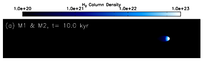
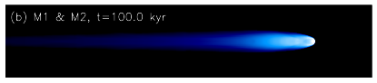
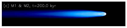
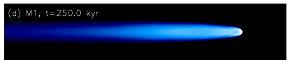
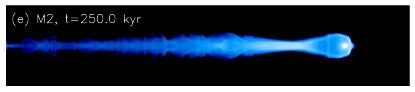
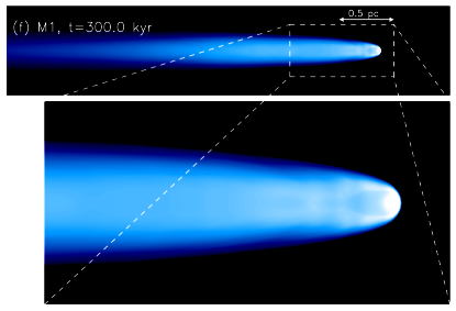
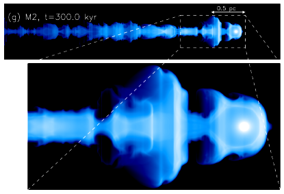
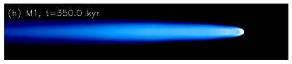
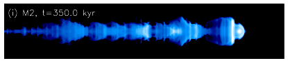
Figure 5.— Time sequence of H₂ column density (i. e., of the material from Mira’s wind), for models M1 and M2. The value of the column density can be read from the logarithmic gray-scale bar (color-scale in the on-line version) at the top of the plots. The time of evolution is indicated in the legend at the upper left corner of each panel. For the first three panels (a–d) the evolution is identical for both models. We have included a blow-up of the region close to the wind source for an integration time of $300~{}\mathrm{kyr}$ (f and g). The physical size is indicated by the arrows in panels (f) and (g).

One problem of interpreting the Martin et al. (2007) observations of Mira is that the broad band filters in GALEX do not give much information about the physical mechanisms that produce the observed emission. They suggested that the bulk of the emission arises from H₂ molecules, which are likely to be present in the cold wind of Mira, but not in the surrounding environment.

In order to make a better comparison with the observations we have added a passive scalar in the simulations that allows us to identify the material from Mira’s wind and the ISM material. We then computed column density maps of the material from Mira’s wind (which would be molecular H₂) and present them in the form of a time sequence in Figure 5.

In Figure 5 we see that the tail forms and reaches the observed length (of Mira’s comet) after approximately $\sim 300~{}\mathrm{kyr}$. The ISM that enters from the right changes (in model M2) to the Local Bubble parameters at $t=200~{}\mathrm{kyr}$, but it takes some $\sim 5~{}\mathrm{kyr}$ to reach the two-wind interaction region. From then on, models M1 and M2 start to differ.

From the column density maps it is clear that the stellar wind material in M1 is well confined to a region that resembles the tail of Mira for the duration of the simulation, but (as we have discussed above) this requires an ambient density that puts the axial standoff distance too close to Mira.

For model M2, as Mira crosses into the Local Bubble its wind expands towards a new steady state configuration (which is not reached in our simulations). We found that at after only $20\mathrm{kyr}$ the stellar wind has expanded enough to form a dense structure extending ${\sim 2\times 10^{17}~{}\mathrm{cm}}$ upstream from the stellar wind source. This size is in agreement with the axial extend of the head of Mira’s comet. We also see that the tail in model M2 expands at a much slower rate compared to the head, therefore reproducing the “broad head/narrow tail” morphology of Mira’s comet for a timescale on the order of $100~{}\mathrm{kyr}$. After $150~{}\mathrm{kyr}$ inside the Local Bubble the tail of Mira has expanded laterally beyond what is observed in the GALEX UV maps (see Martin et al. 2007, and diagram in Fig. 1).

To simulate the UV emission that would arise from the H₂ molecules requires a chemical/radiation transfer calculation that is beyond the scope of this paper. We only note that if we use the standard conversion factor $A_{\mathrm{V}}\approx 10^{-21}N_{\mathrm{H}}$ (due to dust absorption), we find that the tail in our simulations has $A_{\mathrm{V}}\sim 10$. Therefore, molecules present in the wind from Mira A would not be photodissociated in a substantial way, and the tail should indeed have a large H₂ fraction.

Two interesting issues arise from this work, one is the age of Mira’s tail itself, the other is how long it has been inside the Local Bubble (assuming that this is the case).

Regarding the age of the tail, in the original discovery of Martin et al. (2007), the authors estimate that the tail was formed in approximately $30~{}\mathrm{kyr}$, while the simulations of Wareing et al. (2007) suggested an age of $450~{}\mathrm{kyr}$. This large discrepancy is related to the rate at which Mira’s wind decelerates to merge dynamically with the ISM. Martin et al. (2007) assumed that the wind material instantly decelerates, so the $30~{}\mathrm{kyr}$ is the time that Mira takes to traverse the length of the tail. In contrast, the $450~{}\mathrm{kyr}$ timescale of Wareing et al. (2007) was directly obtained from numerical simulations which are, however, sensitive to viscous effects. Such effects depend mainly on two things: the density of the ISM that is used (a physical effect), and the amount of artificial viscosity (a numerical effect) needed to stabilize the code. Artificial viscosity usually overwhelms real viscosity, resulting in an enhanced deceleration, thus the numerical estimates correspond to lower limits of the actual age. Our simulations lie in between these two previous estimates, as they require a time of $\sim 300~{}\mathrm{kyr}$ to develop Mira’s tail. This difference with the model of Waering et al. (2007) is due to the higher ISM density of our models, which results in a higher deceleration rate.

The question of the time spent by Mira inside the Local Bubble is not well constrained by our models because the tail takes on the order of $100~{}\mathrm{kyr}$ to expand laterally in an appreciable way. Our results suggest that Mira could have crossed into the Local Bubble between $20$ and $120~{}\mathrm{kyr}$ ago. This result is in rough agreement with the $130$-$225~{}\mathrm{kyr}$ proposed by Wareing et al. (2007). In this respect, a more detailed map of the Local Bubble and an extrapolation of Mira’s motion might prove more useful.

5. Summary

We have modeled the cometary structure observed around Mira as the interaction of the cold, dense wind from Mira A with a streaming ISM. For this purpose we have used a newly developed code, which is described in detail in the Appendix. Similar simulations have been done previously (Wareing et al., 2007; Raga et al., 2008), but they fail to reproduce the broad-head/narrow-tail configuration characteristic of Mira’s comet.

The new element in our simulations is to assume that Mira has recently crossed (from a denser than previously considered) medium into the Local Bubble, a region of tenuous coronal gas. This possibility was first suggested by Wareing et al. (2007), and is quite feasible given Mira’s current location.

By starting a stellar wind in a denser region than previous papers we are able to reproduce the width of the observed tail of Mira’s comet. By allowing the stellar wind source to enter (at a later time) a less dense region of the ISM (i. e., the Local Bubble) we obtain an expansion of the cometary head. For the parameters of our model, the predicted cometary structure has a striking resemblance to Mira’s comet after $\sim 20~{}\mathrm{kyr}$ time after entering the Local Bubble, and the structure last for another $\sim 100~{}\mathrm{kyr}$.

The age that we obtain for the formation of the tail is $\mathrm{\sim 300~{}\mathrm{kyr}}$. This can be compared with estimates by Martin et al. (2007, $30~{}\mathrm{kyr}$) and by Wareing et al. (2007, $\mathrm{450~{}\mathrm{kyr}}$), that assume either total, or very little (respectively) deceleration of the wind as it encounters the ISM.

We should note that Meaburn et al. (2009) recently discovered a bipolar jet system in the Mira system (possibly ejected from Mira B). This collimated outflow might have an important effect in the formation of Mira’s cometary head and tail, which has not been considered in our present work, and should clearly be studied in the future.

Appendix A The walicxe code

Our previous adaptive grid codes (e. g., the yguazú-a, see Raga et al. 2000) were not suited for running in parallel computers with distributed memory (i.e. clusters). In order to achieve high resolution by today’s standards we have developed the new code walicxe, which contains the cooling/chemistry modules of yguazú-a, but uses a new adaptive mesh designed to be easily parallelizable in clusters. At this point we only have a 2D version, with a 3D version in progress. We describe below the numerical algorithm and the AMR scheme of the walicxe code.

A.1. Basic equations

The 2D Euler system of equations can be written in Cartesian coordinates as:

$$\frac{\partial\mathbf{U}}{\partial t}+\frac{\partial\mathbf{F}}{\partial x}+\frac{\partial\mathbf{G}}{\partial y}=\mathbf{S},$$ (A1)

where

$$\mathbf{U}=\left[\begin{array}[]{c}\rho\\ \rho u\\ \rho v\\ E\\ n_{1}\\ n_{2}\\ \vdots\\ n_{r}\end{array}\right],~{}~{}\mathbf{F}=\left[\begin{array}[]{c}\rho u\\ P+\rho u^{2}\\ \rho uv\\ u(E+P)\\ n_{1}u\\ n_{2}u\\ \vdots\\ n_{r}u\end{array}\right],~{}~{}\mathbf{G}=\left[\begin{array}[]{c}\rho v\\ \rho vu\\ P+\rho v^{2}\\ v(E+P)\\ n_{1}v\\ n_{2}v\\ \vdots\\ n_{r}v\end{array}\right],~{}~{}\mathrm{and}~{}~{}\mathbf{S}=\left[\begin{array}[]{c}0\\ 0\\ 0\\ G-L\\ S_{1}\\ S_{2}\\ \vdots\\ S_{r}\end{array}\right].$$ (A2)

$\mathbf{U}$ are the so-called conserved variables, $\rho$ is the mass density, $(u,v)$ are the velocity components in the $(x,y)$-directions, $n_{1},n_{2},...,n_{r}$ are densities of additional species that are advected passively into the fluid, which can be used to compute heating/cooling rates. $\mathbf{F}$ and ${\mathbf{G}}$ are the fluxes in the $x$ and $y$ directions, respectively;

$$P=\left(n_{i}+n_{e}\right){kT}$$ (A3)

is the thermal pressure, and the (total) energy is given by

$$E=\frac{1}{2}\rho\left(u^{2}+v^{2}\right)+C_{v}P,$$ (A4)

where $C_{v}$ is the specific heat at constant volume. $\mathbf{S}$ is the source vector, that contains the energy gains and losses ($G$ and $L$, from radiative and collisional processes) and the reactions rates for the $n_{1},n_{2},...n_{r}$ species, the source vector can be also extended to include geometrical terms for cylindrical and spherical coordinate systems. In addition, one can define a vector with the so-called primitive variables

$$\mathbf{W}=\left[\begin{array}[]{c}\rho\\ u\\ v\\ P\\ n_{1}\\ n_{2}\\ \vdots\\ n_{r}\end{array}\right],$$ (A5)

which are easily obtained from the conserved variables.

A.2. Discretization: finite-areas

We will denote the indices and grid spacings of the computational cells in the $x,~{}y$-directions by $i,~{}j$ and $\Delta x,~{}\Delta y$, respectively. The time is discretized with an index $n$ such that $\Delta t_{n}=t_{n+1}-t_{n}$, which in principle varies at each time-step, however to make the notation clearer we will drop the sub-index $n$ from $\Delta t_{n}$.

Integration of equation A1 on the area of the computational cell centered at $i~{},j$, on a time interval $[t+\Delta t]$ yields the following exact expression:

$$\mathbf{U}_{i,j}^{n+1}=\mathbf{U}_{i,j}^{n}-\frac{\Delta t}{\Delta x}\left(\mathbf{F}_{i+1/2,j}^{n+1/2}-\mathbf{F}_{i-1/2,j}^{n+1/2}\right)-\frac{\Delta t}{\Delta y}\left(\mathbf{G}_{i,j+1/2}^{n+1/2}-\mathbf{G}_{i,j-1/2}^{n+1/2}\right)+\Delta t\mathbf{S}_{i,j}^{n+1/2},$$ (A6)

where the variables $\mathbf{U}_{i,j}^{n}$ are now area averages at a time $t=t_{n}$:

$$\mathbf{U}_{i,j}^{n}=\frac{1}{\Delta x\Delta y}\int_{y-1/2}^{y+1/2}\int_{x-1/2}^{x+1/2}\mathbf{U}\left(x,y,t_{n}\right)\,dx\,dy,$$ (A7)

where $x\pm 1/2=x_{i}\pm\Delta x/2$, $y\pm 1/2=y_{i}\pm\Delta y/2$ are the locus of the boundaries of the cell at $x_{i},~{}y_{j}$. The fluxes are now time (and length) averages:

$$\mathbf{F}_{i+1/2,j}^{n+1/2}=\frac{1}{\Delta y\Delta t}\int_{t_{n}}^{t_{n+1}}\int_{y-1/2}^{y+1/2}\mathbf{F}\left(x_{i+1/2},y,t\right)\,dy\,dt,$$ (A8)

$$\mathbf{G}_{i,j+1/2}^{n+1/2}=\frac{1}{\Delta x\Delta t}\int_{t_{n}}^{t_{n+1}}\int_{x-1/2}^{x+1/2}\mathbf{G}\left(x,y_{j+1/2},t\right)\,dx\,dt.$$ (A9)

And the source terms are time and area averages:

$$\mathbf{S}_{i,j}^{n+1/2}=\frac{1}{\Delta x\Delta y\Delta t}\int_{t_{n}}^{t_{n+1}}\int_{y-1/2}^{y+1/2}\int_{x-1/2}^{x+1/2}\mathbf{S}\left(x,y,t\right)\,dx\,dy\,dt.$$ (A10)

The method we have described if often referred to as finite-volumes, but since we are dealing with 2D it is more accurate to call it finite-areas. Of course, the expressions of eqs. (A6)–(A10) are easily extended to three dimensions yielding a truly finite-volumes method, where the area integrals used above become volume integrals, and the length integrals become surface integrals. What remains now, is to find approximations to the numerical intercell fluxes ($\mathbf{F}_{i+1/2,j}^{n+1/2},~{}\mathbf{G}_{i,j+1/2}^{n+1/2}$) and sources ($\mathbf{S}_{i,j}^{n+1/2}$). This can be done by solving the Riemann problem at the cell interfaces, that is, assuming a true discontinuity of the hydrodynamic variables at such interfaces (Toro, 1999).

A.3. Solution method: Finite areas, second order Godunov scheme

We use a second order Gudunov type method to advance the solution, it uses a linear reconstruction (with slope limiters) of the primitive variables and an approximate Riemann solver to compute the fluxes at the intercell boundaries. As it is customary, below we explain the method in one dimension, the expressions for the fluxes in the $y$-direction are analogous to those in the $x$-direction. The finite-volume (finite-lengths in 1D) solution is:

$$\mathbf{U}_{i}^{n+1}=\mathbf{U}_{i}^{n}-\frac{\Delta t}{\Delta x}\left(\mathbf{F}_{i+1/2}^{n+1/2}-\mathbf{F}_{i-1/2}^{n+1/2}\right)+\Delta t\mathbf{S}_{i}^{n+1/2},$$ (A11)

To obtain a second order approximation of the intercell fluxes we proceed as follows. First, we calculate the timestep $\Delta t$ in order to ensure that the standard Courant-Friedrichs-Lewy condition (Courant et al., 1967) is met. Then, a first order half-timestep is computed as:

$$\mathbf{U}_{i}^{n+1/2}=\mathbf{U}_{i}^{n}-\frac{\Delta t}{2\Delta x}\left(\mathbf{F}_{i}^{n}-\mathbf{F}_{i-1}^{n}\right)+\frac{\Delta t}{2}\mathbf{S}_{i}^{n},$$ (A12)

where the fluxes are obtained solving the Riemann problem with an approximate Riemann solver (see Toro, 1999), using the primitive variables $\mathbf{W}_{i}(\mathbf{U}_{i})$. That is

$$\mathbf{F}_{i}=\mathrm{Riemann}\left(\mathbf{W}_{i},\mathbf{W}_{i+1}\right).$$ (A13)

With the values of $\mathbf{U}_{i}^{n+1/2}$ from eq. (A12) we obtain a new set of primitives $\mathbf{W}_{i}^{n+1/2}$. We then use a linear reconstruction to extrapolate them to the cell boundaries

$$\mathbf{W}_{L,i}^{n+1/2}=\mathbf{W}_{i}^{1/2}-\frac{1}{2}\mathrm{avg}\left(\mathbf{W}_{i}^{n+1/2}-\mathbf{W}_{i-1}^{n+1/2},\mathbf{W}_{i+1}^{n+1/2}-\mathbf{W}_{i}^{n+1/2}\right),$$ (A14a)

$$\mathbf{W}_{R,i}^{n+1/2}=\mathbf{W}_{i}^{1/2}+\frac{1}{2}\mathrm{avg}\left(\mathbf{W}_{i}^{n+1/2}-\mathbf{W}_{i-1}^{n+1/2},\mathbf{W}_{i+1}^{n+1/2}-\mathbf{W}_{i}^{n+1/2}\right),$$ (A14b)

where $\mathrm{avg}$ is an averaging function. The choice of this function is made in order to limit the slope used and avoid spurious oscillations. The code has a number of different averaging functions, the most widely known (although the most diffusive) is the $minmod$ function.

The left and right states in eqs. (A14) are used to approximate the fluxes used in eq. (A11):

$$\mathbf{F}_{i+1/2}^{n+1/2}=\mathrm{Riemann}\left(\mathbf{W}_{R,i}^{n+1/2},\mathbf{W}_{L,i+1}^{n+1/2}\right),$$ (A15a)

$$\mathbf{F}_{i-1/2}^{n+1/2}=\mathrm{Riemann}\left(\mathbf{W}_{R,i-1}^{n+1/2},\mathbf{W}_{L,i}^{n+1/2}\right).$$ (A15b)

At this point a new $\Delta t$ is calculated, and we iterate until the desired evolutionary stage is reached. The time step is the same for all blocks, independently of their level of resolution, this has a cost in computing time, and introduces additional numerical viscosity to coarser blocks (because they are effectively run at a smaller Courant number), but it makes easier and more efficient to balance the load among different processors.

As to the Riemann solver used, the default is the HLLC algorithm, an improvement proposed by Toro et al. (1994) to the HLL (Harten et al., 1983) solver, which restores the information of the contact wave into the solver (the C stands for contact). The original HLL is also available in the code, but is rarely used because it is too diffusive. In addition to this solvers we have implemented a hybrid scheme that combines the HLL and HLLC fluxes to fix the so-called carbuncle or shock instability problem, which occurs when strong shocks align with the computational grid. Our HLL-HLLC scheme is very similar to those proposed by Kim et al. (2009); Huang et al. (2010), the description and some tests are given in §A.6 .

A.4. The adaptive grid

The hydrodynamic+rate equations described above are integrated on a binary, block-based computational grid with the following characteristics.

A.4.1 Blocks (patches)

The adaptive mesh was designed to be used parallel computers with distributed memory (i.e. clusters). It consists of a series of “root” blocks with a predetermined (set at compile time) number of cells, $n_{x}\times n_{y}$. Each block can be subdivided in a binary fashion into four blocks with the same number of cells of the parent block. We will refer to these new blocks as “siblings”, which have twice the resolution of their parent block. The maximum number of levels of refinement allowed ($n_{levs}$) is set at compile time. Thus the maximum resolution is $\Delta_{i}=L_{i}/[2^{n_{levs}-1}(n_{i})]$, where $L_{i}$ is the size of the computational mesh on the $ith$ direction (i.e. $i=x,~{}y$). In addition, each block has its own ghost cells, two in each direction for the second order scheme described below, but can be changed to implement higher order schemes. These cells would be communicated with MPI when adjacent blocks are in different processors.

The result is a tree structure (of blocks or patches, not individual cells), the root blocks branch into higher resolutions up to $n_{levs}$. The equations are only solved in “leaf” blocks, that is, only on blocks that are not further refined.

A.4.2 Refinement/coarsening criteria

Before advancing the solution, at every timestep we update the mesh. This is done by sweeping all the leaf blocks, measuring pressure and density gradients on each of them. If either the density or pressure suffer a relative gradient, between two adjacent cells, above a threshold (user defined, typically of $\sim 0.05$) the block is flagged for refinement. In addition, we enforce that neighboring blocks differ at most on one level of refinement, blocks in proximity to a higher resolution that has been marked for further refinement are flagged as well. Coarsening is also controlled by measuring gradients of density and pressure, but with a different tolerance (also user defined, typically of $\sim 1.0$), if all the relative gradients in the block are below this value the block is marked to be coarsen. Coarsening is only allowed when an entire group of four siblings have been marked and it is not impeded by the proximity criterion.

The actual refinement algorithm assigns the same value of the variables in the parent block to all the siblings ($Oth-$order interpolation), whereas the coarsening assigns the mean value of each variable from the four siblings to their parent block.

Additional refinement criteria are easy to implement depending of the problem to be solved. One can, for instance, use a vorticity criteria, refine above a certain value of any variable, in certain fixed regions, or in regions labeled by a passive scalar advected into the flow.

A.4.3 Parallelization and load balancing

Since each of the blocks have the same number of cells, it is straightforward to send different blocks (actually a group of blocks) to different processors. This is achieved with the standard Message Passing Interface (MPI). At every timestep the blocks that share border with other processors communicate their boundaries (ghost cells). Domain decomposition is made following a Hilbert ordering in similar fashion to the Ramses code (Teyssier, 2002). Each block is assigned a number according to its position in a Hilbert curve of the $n_{levs}-1$ order. Following such curve, the number of leaf blocks is divided evenly among the available processors, and the blocks are distributed to be solved. The tree structure is copied entirely to every processor, but only the leaf blocks are distributed. This, however, is a time consuming operation, and the work-load is only balanced every $n_{load}$ timesteps (user defined typically $n_{load}\sim 10-100$), yielding an overhead of about $10$ percent, depending on how fast the mesh structure changes on a particular problem.

A.5. Testing the code

Several standard tests have been made to the code, we present here one that we believe is very illustrative: the classic double Mach reflection test problem proposed by Woodward & Colella (1984). The test was inspired on laboratory studies and consists of a planar shock that meets a reflecting surface at an angle of $\pi/3$. The reflecting surface is taken to be the $x-$axis, and the initial conditions (explained in all detail in Woodward & Colella 1984) of the problem are:

$$\left(\rho,u,v,P\right)=\left\{\begin{array}[]{ll}\left(1.4,~{}0,~{}0,~{}1\right)&~{}~{}~{}\mathrm{for}~{}x>x_{s},\\ \left(8,~{}8.25\sin\alpha,~{}-8.25\cos\alpha,~{}116.5\right)&~{}~{}~{}\mathrm{otherwise.}\\ \end{array}\right.$$ (A16)

which correspond to a Mach 10 shock in air (using an adiabatic equation of state with $C_{v}=2.5$, $\gamma=1.4$). The problem is solved on a Cartesian domain $[0,4]\times[0,1]$ with the following boundary conditions: outflow boundaries in $x=4$; reflective boundaries in $y=0$ for $x>1/6$; at $x=0$, and $y=0$ for $x<1/6$ inflow conditions are used; at $y=1$ time dependent inflow conditions are applied, tracing the position of the shock front that moves according to $x_{s}(t)=1/6+10\,y\sin\alpha+y\tan\alpha$. The flow configuration produces a series of shocks, two of which are almost perpendicular and are separated by a contact discontinuity, and a small jet at the base of the reflecting surface. This jet is driven by a pressure gradient and its evolution is known to be very sensitive to numerical diffusion. The results of this test can be compared with those of Woodward & Colella (1984), and many other codes which have adopted it as a standard test for two dimensional hydrodynamics (e.g. Mignone et al. 2007; Stone et al. 2008).

In Figure 6, we show the results of the double Mach reflection test with the HLLC solver, for an integration time of $t=0.2$, for two different resolutions. Both runs start with 4 square root blocks aligned along the $x$-axis. The root blocks have $10\times 10$ cells, covering a physical size of $(1\times 1)$. The run in panel (a) has $5$ levels of refinement, for a maximum resolution of $\Delta x=\Delta y=1/160$; the run in panel (b) has $6$ levels of refinement, and a maximum resolution of $\Delta x=\Delta y=1/320$. Below each of the panels, the AMR structure (only the $[0,3]\times[0,1]$ region) is shown, each square corresponds to one $n_{x}\times n_{y}$ block, and in color we show the domain decomposition in $8$ processors. Notice how the mesh is only refined at places where the flow properties change, and it remains coarse at regions where the flow is smooth.

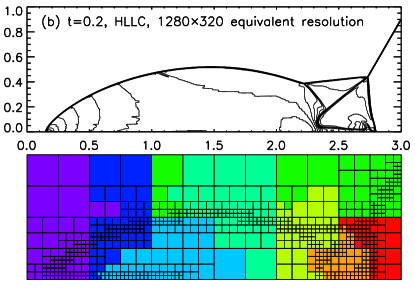
Figure 6.— Density contours and computational mesh at $t=0.2$ for the double Mach reflection test, with the HLLC solver, at two different resolutions. The computational domain is $[0,4]\times[0,1]$, but for visual purposes we only display the $[0,3]\times[0,1]$ region. The equivalent resolution at the finest level is indicated in each panel. Below the contours we show the AMR blocks (each of $10\times 10$ cells), and with colors we indicate the different processors in which the work load was distributed at the time.

Another feature that can be identified is the fact that the jet formed along the reflecting surface (at $x\sim 2.4$–$2.8$) reaches the shock that is almost perpendicular to the surface ($x\sim 2.8$), bending it slightly at its base. This is often called “the kinked Mach stem”, and it is unphysical, caused by insufficient numerical diffusion at places where shocks closely align with the computational grid (Quirk, 1994). This issue becomes particularly critical for high resolution simulations (less numerical/artificial viscosity).

A.5.1 Parallel performance

Is is customary to measure the performance of a parallel code in terms of its scaling with the number of processors. Ideally the computing time would scale as $\propto 1/N_{p}$, where $N_{p}$ is the number of processors. In fact, many fixed grid codes show near ideal scaling. The reason for such a good scaling is twofold: (i) most of the code is parallelizable, which restricts the communication between processors to passing boundaries and determining the timestep, and (ii) since the grid is fixed, each processor knows beforehand with which processors the communication will take place.

Adaptive mesh codes use a significant amount of CPU time to maintain the AMR structure, and neighboring blocks can be in a different processors at different times. This causes AMR codes to scale less than ideally, but the CPU time and memory requirements can remain significantly lower than for fixed grid codes. Also, there are many variables that can impact the performance, and many of them are problem dependent. To illustrate this, we took the double Mach reflection test with an equivalent resolution of $2560\times 640$ cells and ran it on $2$, $4$, $8$, $16,$ and $32$ processors. To achieve the same resolution at the highest level of refinement we used three combinations: $5$ levels of refinement with $40\times 40$ cells blocks, $6$ levels with blocks of $20\times 20$ cells, and $7$ levels with $10\times 10$ blocks, the scaling results are presented in Figure 7.

Figure 7.— Scaling of the Walicxe code for the double Mach reflection test at an equivalent resolution of $2560\times 640$ cells, on 2, 4, 8, 16, and 32 processors. The different symbols are for a different combination of levels of refinement and block size, as indicated in the legend. We have included (dashed line) the ideal $\propto 1/N_{p}$ scaling for reference.

We see from the figure a good performance of the code, almost linear for a small number of processors. As we increase the number of processors the portion of domain that is solved by each processors becomes too small and the communication time becomes important compared to the time to solve each region. Certainly, if we require an even finer resolution, the transition from ideal, to not-so-ideal would happen at a larger number of processors.

Is is quite noticeable that by allowing the mesh to be finer the CPU time drops dramatically. We must note that the outcome is particularly good because the problem is well suited for an adaptive mesh, the regions of sharp changes are well localized and are a small portion of the entire computational domain. If refinement is required in a larger portion of the domain, larger blocks and a small number of levels would be beneficial.

A.6. Fixing the kinked Mach stem (“carbuncle”) problem

The so-called numerical shock instability, or “carbuncle” problem was first reported by Quirk (1994), and although a full understanding of the instability and its cure is not reached (Liou, 2000; Nishikawa & Kitamura, 2008), researchers seem to agree that the culprit is insufficient viscosity when shocks align with the computational cell interfaces. Also, Riemann solvers that perform exceptionally well on shear layer problems (such as the Roe solver, Roe 1981) suffer more of this pathology, while more diffusive ones, such as the HLL solver have been considered virtually carbuncle-free. In recent years, several remedies have been put forward to solve this instability, most of them for the solver of Roe (see for instance Nishikawa & Kitamura, 2008). Among the remedies, a family of methods is to produce hybrid fluxes, combining a solver that is more diffusive, such as the HLL, with a more accurate, yet carbuncle-prone solver. In particular (Kim et al., 2009; Huang et al., 2010), have proposed a combination of the HLL and HLLC fluxes. We have implemented a similar hybrid flux formed by a linear combination of the two fluxes

$$\mathbf{F}_{\mathrm{HLL-HLLC}}=\beta_{1}\mathbf{F}_{\mathrm{HLLC}}+\beta_{2}\mathbf{F}_{\mathrm{HLL}},$$ (A17)

where the $\beta_{1}+\beta_{2}=1$, these coefficients are chosen in order to give more weight to the HLLC solver when shear flows are present, and to the HLL in the presence of strong shocks aligned with the grid. To do this we check the direction of the velocity difference vector between the left and right states: $\mathbf{\Delta q}=(u_{R}-u_{L},v_{R}-v_{L})$. In particular we use the magnitude of the projection of the unit vector in the direction of $\mathbf{\Delta q}$ with the unit vector normal to the cell interface, that is : $\alpha_{1}=|u_{R}-u_{L}|/[(u_{R}-u_{L})^{2}+(v_{R}-v_{L})^{2}]^{1/2}$. After some tests, we choose $\beta_{1}=\sqrt{\alpha}_{1}$, in figure 8 we compare of the results from the double Mach reflection test with the HLLC, HLL, and HLL-HLLC solvers, all at $t=0.2$, and all with the same equivalent resolution $\Delta x=\Delta y=1/(640)$.

Figure 8.— Density maps for the $[2.25,2.75]\times[0,0.5]$ region of the double Mach reflection test with the (a) HLLC, (b) the HLL, and (c) the hybrid HLL-HLLC Riemann solvers. The density values are indicated by the bar at the right. All the runs were done with a maximum resolution of $\Delta x=\Delta y=1/(640)$.

We can see from the Figure (panel a) how the HLLC solver alone produces a kinked Mach stem, but resolves sharply the contact discontinuity (the density change at an angle of $~{}40\deg$. In fact some Kelvin-Helmholtz “rolls” start to appear, along this discontinuity and extend to the jet propagating along the reflecting surface ($x$-axis). For the HLL solver (panel b) the kinked Mach stem is controlled (barely noticeable), but the diffusion at the contact surfaces is evident, producing a smeared solution compared to the more accurate HLLC solver. In panel (c) we show the results with the hybrid fluxes, and the best of the other two solvers is evident, a barely noticeable kinked Mach stem, with a sharp contact surface.

References

- Cantó & Raga (1991) Cantó, J., & Raga, A. C. 1991, ApJ, 372, 646
- Cantó et al. (1996) Cantó, J., Raga, A. C., & Wilkin, F. P. 1996, ApJ, 469, 729
- Courant et al. (1967) Courant, R., Friedrichs, K., & Lewy, H. 1967, IBM Journal of Research and Development, 11, 215
- Evans (1967) Evans, D. S. 1967, in IAU Symposium, Vol. 30, Determination of Radial Velocities and their Applications, ed. A. H. Batten & J. F. Heard, 57
- Harten et al. (1983) Harten, A., Lax, P. D., & van Leer, B. 1983, SIAM review, 25, 357
- Huang et al. (2010) Huang, K., Wu, H., Yu, H., & Yan, D. 2010, International Journal for Numerical Methods in Fluids
- Kim et al. (2009) Kim, S. D., Lee, B. J., Lee, H. J., & Jeung, I. 2009, Journal of Computational Physics, 228, 7634
- Knapp et al. (2003) Knapp, G. R., Pourbaix, D., Platais, I., & Jorissen, A. 2003, A&A, 403, 993
- Lallement et al. (2003) Lallement, R., Welsh, B. Y., Vergely, J. L., Crifo, F., & Sfeir, D. 2003, A&A, 411, 447
- Liou (2000) Liou, M. 2000, Journal of Computational Physics, 160, 623
- Martin et al. (2007) Martin, D. C., Seibert, M., Neill, J. D., Schiminovich, D., Forster, K., Rich, R. M., Welsh, B. Y., Madore, B. F., Wheatley, J. M., Morrissey, P., & Barlow, T. A. 2007, Nature, 448, 780
- Matthews et al. (2008) Matthews, L. D., Libert, Y., Gérard, E., Le Bertre, T., & Reid, M. J. 2008, ApJ, 684, 603
- Meaburn et al. (2009) Meaburn, J., López, J. A., Boumis, P., Lloyd, M., & Redman, M. P. 2009, A&A, 500, 827
- Mignone et al. (2007) Mignone, A., Bodo, G., Massaglia, S., Matsakos, T., Tesileanu, O., Zanni, C., & Ferrari, A. 2007, ApJS, 170, 228
- Nishikawa & Kitamura (2008) Nishikawa, H., & Kitamura, K. 2008, Journal of Computational Physics, 227, 2560
- Perryman et al. (1997) Perryman, M. A. C., Lindegren, L., Kovalevsky, J., Hoeg, E., Bastian, U., Bernacca, P. L., Crézé, M., Donati, F., Grenon, M., van Leeuwen, F., van der Marel, H., Mignard, F., Murray, C. A., Le Poole, R. S., Schrijver, H., Turon, C., Arenou, F., Froeschlé, M., & Petersen, C. S. 1997, A&A, 323, L49
- Quirk (1994) Quirk, J. J. 1994, International Journal for Numerical Methods in Fluids, 18, 555
- Raga & Cantó (2008) Raga, A. C., & Cantó, J. 2008, ApJ, 685, L141
- Raga et al. (2008) Raga, A. C., Cantó, J., De Colle, F., Esquivel, A., Kajdic, P., Rodríguez-González, A., & Velázquez, P. F. 2008, ApJ, 680, L45
- Raga et al. (2000) Raga, A. C., Navarro-González, R., & Villagrán-Muniz, M. 2000, Revista Mexicana de Astronomia y Astrofisica, 36, 67
- Raga & Reipurth (2004) Raga, A. C., & Reipurth, B. 2004, Revista Mexicana de Astronomia y Astrofisica, 40, 15
- Roe (1981) Roe, P. L. 1981, Journal of Computational Physics, 43, 357
- Ryde et al. (2000) Ryde, N., Gustafsson, B., Eriksson, K., & Hinkle, K. H. 2000, ApJ, 545, 945
- Stone et al. (2008) Stone, J. M., Gardiner, T. A., Teuben, P., Hawley, J. F., & Simon, J. B. 2008, ApJS, 178, 137
- Teyssier (2002) Teyssier, R. 2002, A&A, 385, 337
- Toro (1999) Toro, E. F. 1999, Riemann Solvers and Numerical Methods for Fluid Dynamics (Springer)
- Toro et al. (1994) Toro, E. F., Spruce, M., & Speares, W. 1994, Shock Waves, 4, 25
- Turon et al. (1993) Turon, C., Creze, M., Egret, D., Gomez, A., Grenon, M., Jahreiß, H., Requieme, Y., Argue, A. N., Bec-Borsenberger, A., Dommanget, J., Mennessier, M. O., Arenou, F., Chareton, M., Crifo, F., Mermilliod, J. C., Morin, D., Nicolet, B., Nys, O., Prevot, L., Rousseau, M., Perryman, M. A. C., & et al. 1993, Bulletin d’Information du Centre de Donnees Stellaires, 43, 5
- Ueta (2008) Ueta, T. 2008, ApJ, 687, L33
- Vergely et al. (2001) Vergely, J., Freire Ferrero, R., Siebert, A., & Valette, B. 2001, A&A, 366, 1016
- Wareing et al. (2007) Wareing, C. J., Zijlstra, A. A., O’Brien, T. J., & Seibert, M. 2007, ApJ, 670, L125
- Wilkin (1996) Wilkin, F. P. 1996, ApJ, 459, L31
- Woodward & Colella (1984) Woodward, P., & Colella, P. 1984, Journal of Computational Physics, 54, 115
- Young (1995) Young, K. 1995, ApJ, 445, 872