Statistics of layered zigzags: a two–dimensional generalization of TASEP

Abstract

A novel discrete growth model in 2+1 dimensions is presented in three equivalent formulations: i) directed motion of zigzags on a cylinder, ii) interacting interlaced TASEP layers, and iii) growing heap over 2D substrate with a restricted minimal local height gradient. We demonstrate that the coarse–grained behavior of this model is described by the two–dimensional Kardar–Parisi–Zhang equation. The coefficients of different terms in this hydrodynamic equation can be derived from the steady state flow–density curve, the so called ‘fundamental’ diagram. A conjecture concerning the analytical form of this flow–density curve is presented and is verified numerically.

PACS numbers: 05.40.-a, 05.70.Np, 68.35.Fx

It is well established in the last two decades beijeren ; pischke ; majumdar ; kk that the one–dimensional Kardar–Parisi–Zhang (KPZ) equation KPZ adequately describes the long–range dynamics of a collective motion of hopping particles on a line known as ”Asymmetric Simple Exclusion Process” (ASEP) spitzer ; liggett ; spohn ; dhar . Apart from many fruitful theoretical advantages, this ASEP–to–KPZ mapping enables a fast and simple way of modelling the KPZ dynamics. The latter is of wide interest since it appears in various contexts, (provided the symmetry of a nonequilibrium statistical system under discussion allows for the effective 1+1–dimensional description), including, to name but a few, the models of crystal growth RSOS , Molecular Beam Epitaxy MBE , Burgers’ turbulence zhang ; khanin , polynuclear growth M ; PS ; PNG ; BR ; J , ballistic deposition Mand ; MRSB ; KM ; BMW etc.

It is therefore an appealing idea to seek for a similar simple discrete multi–particle system whose long–range dynamics would be governed by a two–dimensional KPZ–type equation. Lately, several models of the desired nature, i.e. ones which combine the discreteness with the long–range KPZ–type dynamics, were suggested wolf ; prsp ; borodin1 ; borodin2 ; borodin3 ; odor . In this Letter we propose another model belonging to this class, which, in our opinion, combines the advantage of physical transparency with the flexibility of tuning the internal parameters of the model to catch the different desired regimes both in 1+1 and in 2+1 dimensions. This model, which we call “Zigzag Model”, has a simple geometrical formulation.

Take an infinite cylinder covered by tilted square grid as shown in Fig.1a,b and consider a directed closed path (“zigzag”) around a cylinder. Any such path consists of a constant number of rises and descents, constituting “kinks” (here and below we conventionally define rises and descents with respect to a rightward step). The density of descents, $\rho$, is defined by the tilt angle $\alpha$ – see Fig.1a,b where this density equals $\rho=1/2$ (for $\tan\alpha=1$) and $\rho=1/4$ (for $\tan\alpha=1/3$), respectively. Consider evolution of a system of such nonintersecting zigzags. At each infinitesimal time step $dt$ any elementary kink oriented downwards, can turn upwards with probability $p\,dt$ under the condition that such a move is not blocked by the upper nearest neighboring zigzag (i.e. all zigzags stay nonintersecting at all times). By an appropriate rescaling of time, $t$, we set $p\equiv 1$. The examples of elementary jumps which are allowed and those which are blocked are shown in Fig.1.

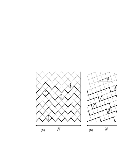
Figure 1: The zigzags on a cylinder for different tilt angles $\alpha=\pi/4$ (a) and $\alpha=\arctan(1/3)$ (b), the examples of allowed an forbidden moves are shown.

For better understanding of the dynamics of the model, notice that the evolution of a separated zigzag, (if, for the time being, we neglect its interaction with the other ones), can be interpreted as a hopping dynamics in a standard one–dimensional Totally Asymmetric Simple Exclusion Process (TASEP) pischke – see Fig.2 for the corresponding mapping, which is both conventional and self–explanatory. Essentially, a descent (rise) in a zigzag is identified with a particle (hole) in the corresponding TASEP. Therefore, the set of zigzags can be viewed as a system of interacting TASEP layers.

The connection between zigzags and TASEP layers is shown in Fig.2a. Here, there are two sorts of constraints on the movement of the particles in layer $B_{2}$. Indeed, for a jump to be possible at some point of the $A_{2}$ zigzag, two conditions should be simultaneously fulfilled: i) it should be a downward kink, and ii) the movement should not be blocked by the upper zigzag. The translation of the first condition into the TASEP language is convenient: there should be a particle at a given position in $B_{2}$ and a void immediately to the right of it. In turn, the second rule (i.e., the one describing the interaction of the $B_{1}$ and $B_{2}$ layers) can be formulated as follows: it is possible to label the particles in the layers $B_{1}$ and $B_{2}$ in a way such that the $k$th particle in the layer $B_{2}$ can never surpass the particle with the same label (i.e., the $k$-th one) in the upper layer $B_{1}$, giving rise to an “interlaced TASEP” picture shown in Fig.2b endnote2 .

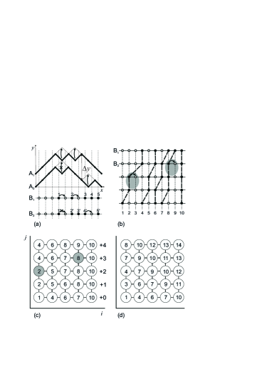
Figure 2: The interconnections between zigzag, interacting TASEP and tag diffusion representations of the model. a) Interaction of two zigzags and the two corresponding TASEP layers, examples of the same allowed and forbidden moves are shown in both representations; b) interacting TASEP layers with examples of allowed moves the bold dashed lines connect the particles with the same number (see explanation in the text); c) the system of tagged particles corresponding to the TASEP layers depicted in figure (b), with the same allowed moves highlighted; d) the result of the shift $h_{i,j}\to h_{i,j}+j$.

To prove these jumping rules, consider the distance $\Delta y$ between the zigzags $A_{1}$ and $A_{2}$ (see Fig.2a). At two adjacent spatial positions it satisfies

$$\Delta y(x)=\left\{\begin{array}[]{ll}\Delta y(x-1)+1&\mbox{there is a particle at $x-1/2$}\\ &\mbox{on $B_{2}$ and a void on $B_{1}$}\vskip 6.0pt plus 2.0pt minus 2.0pt\\ \Delta y(x-1)-1&\mbox{there is a void at $x-1/2$}\\ &\mbox{on $B_{2}$ and a particle on $B_{1}$}\vskip 6.0pt plus 2.0pt minus 2.0pt\\ \Delta y(x-1)&\mbox{otherwise}\end{array}\right.$$ (1)

Note, that $\Delta y(x)\geq 1$ at all positions. Therefore, for each particle on the upper line there is a “partner” particle on the lower line that cannot surpass it, and this “partnership” is preserved by the elementary moves. Indeed, if there is a particle on the upper line $A_{1}$ in position $x-1/2$ (particle positions are shifted by half–step as compared to the positions of the kinks) and the zigzag–to–zigzag distance at $x$ is $\Delta y(x)$ then each particle on $A_{2}$ jumping from $x-1/2$ to $x+1/2$ will decrease $\Delta y$ by one, and, therefore, up to $(\Delta y-1)$ particles can pass this point without being affected, while the particle number $\Delta y$, which is the desired “partner” particle, will get stacked at $x-1/2$. Moreover, assume now that the upper particle hops from $x-1/2$ to $x+1/2$. For this move to take place, the position $x+1/2$ should be a void before it, thus (compare to Eq.1)

$$\Delta y(x+1)=\left\{\begin{array}[]{ll}\Delta y(x)+1&\mbox{there is a particle at $x+1/2$}\\ &\mbox{on $B_{2}$}\vskip 6.0pt plus 2.0pt minus 2.0pt\\ \Delta y(x)&\mbox{otherwise}\end{array}\right.$$ (2)

and $\Delta y(x+1)$ does not change as a result of the move. In both cases of (2) the “partner” particle after the move is still the same: either the distance and the order of particles do not change, or the distance increases but the $(\Delta y+1)$th particle as viewed from the new position is the same as $\Delta y$th from the old position.

In case of a finite cylinder with periodic boundary conditions the “partner” particle can, in principle, lag behind by a whole lap. In this case, one should ensure that the two particles do not interact even if formally they are at the same place, so one should keep track of the “real” distances between the particles (i.e., those which correspond to the distances between the kinks on the original cylinder), not the ”apparent” modulo $N$ distances (compare to priezzhev ).

There is now evidence of some spatial symmetry in the model: for each given particle there are exactly two other particles, one to the right and one (with the same number) “on top” of it – see the dashed lines connecting the particles of the same number in Fig.2b, which can block its movement via excluded–volume interaction. To better exploit this symmetry, it is convenient to reformulate the model, following the logic of the so-called “tagged particle diffusion” introduced in majumdar in order to show that on a coarse–grained level the ASEP dynamics is subject to the one–dimensional KPZ equation.

Consider a set of $m$ TASEP layers (zigzags) of length $N$ with $n$ particles within each layer. Note that instead of enumerating the cites of TASEP layers and marking which particular cites are filled with particles, one can store the very same information in a different way by enumerating the particles with two indices $i\in[1,n]$, $j\in[1,m]$, and ascribing to each particle a ‘height’ $h_{i,j}$ equal to its position on the corresponding layer (as measured from some arbitrary chosen “1st cite”). It is clear now that locally the values in the $h_{i,j}$ matrix are increasing in $i$ direction and non–decreasing in $j$ direction. To make the model completely symmetric make the transformation (compare NM ) $h_{i,j}\to h_{i,j}+j$ which (see Fig.2c,d) ensures that $h_{i,j}$ is now increasing function in both directions, $i$ and $j$. Under this transformation the dynamic rules become totally symmetric:

$$h_{i,j}\to\left\{\begin{array}[]{ll}h_{i,j}+1&\mbox{with Prob. $dt$, if}\,\left\{\begin{array}[]{l}h_{i+1,j}>h_{i,j}+1\\ h_{i,j+1}>h_{i,j}+1\end{array}\right\}\vskip 6.0pt plus 2.0pt minus 2.0pt\\ h_{i,j}&\mbox{otherwise}\end{array}\right.$$ (3)

One can interpret these rules as the dynamics of a heap growing over a two–dimensional substrate, with an additional constraint of heap gradient being not less than 1 in each of the transverse directions.

To obtain insights about the large scale dynamics it is useful to consider a coarse–grained hydrodynamic description of the model spohn . To describe the model at a coarse–grained level we will henceforth use $(x,y)$ as the spatial coordinates instead of $(i,j)$ in the lattice model. The coarse–grained dynamics can be described by a local ‘smooth’ velocity field $u(x,y,t)$ which is, in fact, nothing but the average (over space–time element $dx\,dy\,dt$) rate of successful hops $h_{i,j}\rightarrow h_{i,j}+1$, i.e. the average probability to find simultaneously $(h_{i+1,j}-h_{i,j})>1$ and $(h_{i,j+1}-h_{i,j})>1$. This value obviously depends on the average slope (or equivalently on the local densities in both directions in the Zigzag model) of the surface in both directions. Similar to the one–dimensional case spohn ; kk we assume that the velocity field $u(x,y,t)$ depends on the space-time coordinates only through the local densities, i.e.,

$$u(x,y,t)\equiv u(\rho_{x}(x,y,t),\rho_{y}(x,y,t))$$ (4)

where $\rho^{-1}_{x}(x,y,t)=\frac{\partial h(x,y,t)}{\partial x}$ and $\rho^{-1}_{y}(x,y,t)=\frac{\partial h(x,y,t)}{\partial y}$ Note that the value $\rho_{x}$ introduced here has a meaning of particle density in the corresponding TASEP layer.

Suppose that the slopes $\rho_{x,y}$ are weakly fluctuating around some average values $\overline{\rho}_{x,y}$, which are determined by the boundary conditions. Introduce the displacement $d(x,y,t)$ of a particle located at $(x,y)$ from its average position at $t=0$:

$$d(x,y,t)=h(x,y,t)-\frac{x}{\overline{\rho}_{x}}-\frac{y}{\overline{\rho}_{y}}$$ (5)

Then, in an analogy with Maj_thesis the local values of $\rho_{x,y}$ and $d$ are connected via

$$\frac{1}{\rho_{x}(x,y,t)}=\frac{1}{\overline{\rho}_{x}}+\frac{\partial d(x,y,t)}{\partial x};\;\frac{1}{\rho_{y}(x,y,t)}=\frac{1}{\overline{\rho}_{x}}+\frac{\partial d(x,y,t)}{\partial y}$$ (6)

Assuming now $\left|\frac{\partial d}{\partial x}\right|\ll 1$ and $\left|\frac{\partial d}{\partial y}\right|\ll 1$ one can expand both $\rho_{x,y}$ and $u(\rho_{x},\rho_{y})$ as power series in the derivatives of $d$, obtaining up to the second order:

$$\begin{array}[]{l}\displaystyle\rho_{x}(x,y,t)=\overline{\rho}_{x}\left(1-\overline{\rho}_{x}\frac{\partial d}{\partial x}+\left(\overline{\rho}_{x}\right)^{2}\left(\frac{\partial d}{\partial x}\right)^{2}+...\right)\vskip 6.0pt plus 2.0pt minus 2.0pt\\ \displaystyle\rho_{y}(x,y,t)=\overline{\rho}_{y}\left(1-\overline{\rho}_{y}\frac{\partial d}{\partial y}+\left(\overline{\rho}_{y}\right)^{2}\left(\frac{\partial d}{\partial y}\right)^{2}+...\right)\end{array}$$ (7)

which when substituted into (5) gives

$$\begin{array}[]{lll}u(\rho_{x},\rho_{y})&=&u(\overline{\rho}_{x},\overline{\rho}_{y})-\displaystyle\overline{\rho}_{x}^{2}u_{x}(\overline{\rho}_{x},\overline{\rho}_{y})\frac{\partial d}{\partial x}-\overline{\rho}_{y}^{2}u_{y}(\overline{\rho}_{x},\overline{\rho}_{y})\frac{\partial d}{\partial y}\vskip 6.0pt plus 2.0pt minus 2.0pt\\ &+&\displaystyle\left(\overline{\rho}_{x}^{3}u_{x}(\overline{\rho}_{x},\overline{\rho}_{y})+\frac{1}{2}\overline{\rho}_{x}^{4}u_{xx}(\overline{\rho}_{x},\overline{\rho}_{y})\right)\left(\frac{\partial d}{\partial x}\vskip 6.0pt plus 2.0pt minus 2.0pt\right)^{2}\vskip 6.0pt plus 2.0pt minus 2.0pt\\ &+&\displaystyle\left(\overline{\rho}_{y}^{3}u_{y}((\overline{\rho}_{x},\overline{\rho}_{y})+\frac{1}{2}\overline{\rho}_{y}^{4}u_{yy}(\overline{\rho}_{x},\overline{\rho}_{y})\right)\left(\frac{\partial d}{\partial y}\vskip 6.0pt plus 2.0pt minus 2.0pt\right)^{2}\vskip 6.0pt plus 2.0pt minus 2.0pt\\ &+&\displaystyle\overline{\rho}_{x}^{2}\overline{\rho}_{y}^{2}u_{xy}(\overline{\rho}_{x},\overline{\rho}_{y})\frac{\partial d}{\partial x}\frac{\partial d}{\partial y}+...\end{array}$$ (8)

where for brevity we introduced the notation $u_{x}$, $u_{y}$, etc. for the partial derivatives $u_{x}=\frac{\partial u}{\partial\rho_{x}},\;u_{y}=\frac{\partial u}{\partial\rho_{y}},...$.

This allows us to write down a time–dependent differential equation for $d$ which belongs to the two–dimensional KPZ class:

$$\begin{array}[]{lll}\frac{\partial d}{\partial t}&=&D\Delta d+\eta+\displaystyle u(\rho_{x},\rho_{y})=D\Delta d+\eta+\displaystyle u(\overline{\rho}_{x},\overline{\rho}_{y})-\vskip 6.0pt plus 2.0pt minus 2.0pt\\ &-&\displaystyle\sum_{\alpha=x,y}a_{\alpha}\,\frac{\partial d}{\partial\alpha}+\sum_{\alpha=x,y}\sum_{\beta=x,y}\,b_{\alpha\beta}\,\frac{\partial d}{\partial\alpha}\,\frac{\partial d}{\partial\beta}\end{array}$$ (9)

where $D$ is a diffusion coefficient, $\eta(x,y,t)$ is the noise term

$$\left<\eta(x,y,t)\right>=0,\;\left<\eta(x,y,t)\eta(x^{\prime},y^{\prime},t^{\prime})\right>=\delta_{x,x^{\prime}}\delta_{y,y^{\prime}}\delta_{t,t^{\prime}}$$ (10)

and $a_{\alpha},\,b_{\alpha\beta}$ for $\{\alpha,\beta\}=x,y$ are:

$$\begin{array}[]{lll}a_{\alpha}&=&\overline{\rho}_{\alpha}^{2}u_{\alpha}(\overline{\rho}_{x},\overline{\rho}_{y}),\vskip 6.0pt plus 2.0pt minus 2.0pt\\ b_{\alpha\alpha}&=&\overline{\rho}_{\alpha}^{3}u_{\alpha}(\overline{\rho}_{x},\overline{\rho}_{y})+\frac{1}{2}\overline{\rho}_{\alpha}^{4}u_{\alpha\alpha}(\overline{\rho}_{x},\overline{\rho}_{y}),\vskip 6.0pt plus 2.0pt minus 2.0pt\\ b_{xy}&=&\overline{\rho}_{x}^{2}\overline{\rho}_{y}^{2}u_{xy}(\overline{\rho}_{x},\overline{\rho}_{y})\end{array}$$ (11)

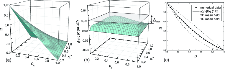
Figure 3: Comparison of the theoretical and numerical results for $u(\rho_{x},\rho_{y})$. a)$u(\rho_{x},\rho_{y})$ dependence as measured by direct numerical simulations (see main text for the details about the simulations); b) the discrepancy between the numerical result for $u$ and the one conjectured in Eq. 15; c) the $u(\rho)$ behavior in the $\rho=\rho_{x}=\rho_{y}$ plane, the points correspond to numerical results, while the dashed line is the naive mean-field guess $u=(1-\rho)^{2}$ (compare Eq. 13) and bold line is the conjectured dependence $u=(1-\rho)(1-\rho/2)$ (compare Eq. 15); .

The behavior of the system is controlled by the usual flow–density dependence $u(\rho_{x},\rho_{y})$, which is central in all models of traffic (see, for example, CSS ) and is usually referred to as the ‘fundamental’ diagram. Indeed, the flow of the particles in the interlaced TASEP formulation of the zigzag model is equal to $I(\rho_{x},\rho_{y})=\rho_{x}u(\rho_{x},\rho_{y})$. Recall that in the 1D–case the function $u(\rho)=I(\rho)/\rho$ is just $u=1-\rho$ and it can be obtained by the mean–field arguments. In absence of interaction between layers one would have expected the same dependence in our model:

$$u(\rho_{x},\rho_{y})=1-\rho_{x}$$ (12)

In the presence of interaction the corresponding 2D mean–field result would be

$$u(\rho_{x},\rho_{y})=(1-\rho_{x})(1-\rho_{y})$$ (13)

where the symmetry of the model is taken into account: a particle can hop if there is a void both in front (with probability $1-\rho_{x}$) and on top (with probability $1-\rho_{y}$) of it and the horizontal and vertical jumps are supposed to be independent. However, contrary to the 1D case, this result is not exact. Indeed, the connectivity of the surface dictates that the local increments $(h_{i+1,j}-h_{i,j)}$ and $(h_{i,j+1}-h_{i,j})$ are positively correlated and cannot be considered as independent.

The exact analytical evaluation of the velocity $u(\rho_{x},\rho_{y})$ up to now is beyond our reach. We have made numerical simulations of $u(\rho_{x},\rho_{y})$, the results being presented in Fig.3. The simulations were performed for the systems of size $N=32$ in both directions with periodic boundary conditions ensuring that the average densities take the values $\overline{\rho}_{x}=\overline{\rho}_{y}=0,\frac{1}{31},\frac{2}{31},...,1$ endnote . The results were averaged over $9\times 10^{6}$ Monte–Carlo steps. To make the comparison with the mean field more visually compelling, we plot in Fig.3c separately the numerical data for $\rho_{x}=\rho_{y}=\rho$ together with the mean–field results (12) and (13). As expected, the first of them overestimates the flow, while the second one underestimates it. In fact, the numerical data fits perfectly the form

$$u(\rho)=(1-\rho)(1-\rho/2)$$ (14)

and the consideration of limiting cases $\rho\rightarrow 0$ and $\rho\rightarrow 1$ suggests that this result may be exact. In particular by developing the perturbation theory at high densities, we are able prove that $u(\rho)\to(1-\rho)/2$ as $\rho\rightarrow 1$, the details of these computations will be published separately preparation .

The simplest generalization of Eq.(14) onto the case of $\rho_{x}\neq\rho_{y}$ which respects the boundary conditions $u(0,0)=1,\,u(1,\xi)=u(\xi,1)=0$ for any $\xi\in[0,1]$ reads

$$u(\rho_{x},\rho_{y})=(1-\rho_{x})(1-\rho_{y})\left(1+\frac{2\rho_{x}\rho_{y}}{(\rho_{x}+\rho_{y})(2-\rho_{x}-\rho_{y})}\right)$$ (15)

In the Fig.3b we have plotted the discrepancy $\Delta u(\rho_{x},\rho_{y})=u_{\rm n}(\rho_{x},\rho_{y})-u(\rho_{x},\rho_{y})$ between numerical, $u_{\rm n}(\rho_{x},\rho_{y})$ and conjectured, $u(\rho_{x},\rho_{y})$, (see (15)) functions. One sees that $u(\rho_{x},\rho_{y})$ is in very good agreement with the results of numerical simulations.

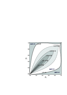
Figure 4: Density plot of the ratio $\lambda_{1}/\lambda_{2}$ of the eigenvalues of the matrix $B$. In the region $\det B<0$ the eigenvalues have opposite signs. Outside the dashed area the system can be regarded as effectively one–dimensional since $\lambda_{1}\gg\lambda_{2}$.

The conjectured function $u(\rho_{x},\rho_{y})$ allows to evaluate the coefficients in (11) for any $\rho_{x}$ and $\rho_{y}$ and to calculate the eigenvalues of the coefficients matrix $b_{\alpha\beta}$ in front of the nonlinear term in Eq.(9). We show thus (see Fig.4) that the domain $[0<\rho_{x}<1,\,0<\rho_{y}<1]$ can be separated into two regions: i) a region where one of the eigenvalues dominates ($|\lambda_{1}|\gg|\lambda_{2}|$) signaling a quasi–one–dimensional behavior, and ii) a region where $|\lambda_{1}|\sim|\lambda_{2}|$ corresponding to the truly two–dimensional KPZ dynamics. In the latter region both eigenvalues are negative, and thus the matrix is positively defined.

Summing up, we have presented a novel model of a statistical driven system in 2+1 dimensions which turned out to be a direct generalization of the conventional one dimensional TASEP model. In the hydrodynamic limit we derived the differential equation for the particle displacement in this model, and we have made a conjecture concerning the flow–on–density dependence of the model (the so called ‘fundamental’ diagram). Clearly, the model suggested here deserves further investigations in various directions. In particular, a detailed investigation of the limiting cases $\rho_{x}=\rho_{y}\rightarrow 0$ and $\rho_{x}=\rho_{y}\rightarrow 1$ can give valuable understanding of the flow–density dependence, the study of the displacement fluctuations in different regimes (compare to majumdar ) should be very fruitful, and the problem of proving conjecture (15) or at least (14) sounds quite challenging. Some progresses in these direction will be reported in a forthcoming longer paperpreparation .

We are grateful to D. Dhar who have coined the idea of the zigzag model in a private discussion with one of us (S.M). It is a pleasure for M.T. to express his gratitude for the hospitality of the LPTMS, Orsay, where the most part of the work has been done.

References

- (1) H. van Beijeren, R. Kutner and H. Spohn, Phys. Rev. Let. 54, 2026 (1985)
- (2) M. Pischke, Z. Racz and D. Liu, Phys. Rev. B 35, 3485 (1987)
- (3) S.N. Majumdar and M. Barma, Phys. Rev. B 44, 5306 (1991)
- (4) For a recent review on this subject see T. Kriecherbauer and J. Krug, J. Phys. A: Math. Theor. 43, 403001 (2010).
- (5) M. Kardar, G. Parisi and Y.C. Zhang, Phys. Rev. Lett. 56, 889 (1986)
- (6) F. Spitzer, Adv. Math. 5, 246 (1970).
- (7) T.M. Liggett, Interacting Particle Systems (Springer-Verlag, New York, 1985).
- (8) H. Spohn, Large Scale Dynamics of Interacting Particles (Springer-Verlag, New York, 1991).
- (9) D. Dhar, Phase Transitions, 9, 51 (1987); L.H. Gwa and H. Spohn, Phys. Rev. A 46, 844 (1992).
- (10) J.M. Kim and J.M. Kosterlitz, Phys. Rev. Lett. 62, 2289 (1989)
- (11) M.A. Herman and H. Sitter, Molecular Beam Epitaxy: Fundamentals and Current, (Springer: Berlin, 1996).
- (12) T. Halpin–Healy and Y.-C. Zhang, Phys. Rep. 254, 215 (1995)
- (13) J. Bec and K. Khanin, Phys. Rep. 447, 1 (2007)
- (14) P. Meakin, Fractals, Scaling, and Growth Far From Equilibrium, (Cambridge University Press: Cambridge, 1998)
- (15) M. Prähofer and H. Spohn, Phys. Rev. Lett. 84, 4882 (2000)
- (16) M. Prähofer and H. Spohn, J. Stat. Phys. 108, 1071 (2002)
- (17) J. Baik and E.M. Rains, J. Stat. Phys. 100, 523 (2000)
- (18) K. Johansson, Comm. Math. Phys. 242, 277 (2003)
- (19) B.B. Mandelbrot, The Fractal Geometry of Nature, (Freeman, New York, 1982)
- (20) P. Meakin, P. Ramanlal, L. M. Sander and R. C. Ball, Phys. Rev. A 34, 5091 (1986)
- (21) J. Krug and P. Meakin, Phys. Rev. A 40, 2064 (1989)
- (22) D. Blomker, S. Maier–Paape and T. Wanner, Interfaces and Free Boundaries 3, 465 (2001)
- (23) D.E. Wolf, Phys. Rev. Lett. 67, 1783 (1991)
- (24) M. Prähofer and H. Spohn, J. Stat. Phys. 88, 999 (1997)
- (25) A. Borodin and P.L. Ferrari, arXiv:0804.3035 (2008)
- (26) A. Borodin and P.L. Ferrari, arXiv:0811.0682 (2008)
- (27) A. Borodin and P.L. Ferrari, Electron. J. Probab. 13, 1380 (2008)
- (28) G. Odor, B. Liedke and K.-H. Heining, Phys. Rev. E 79, 021125 (2009)
- (29) Note that the described system of interlaced TASEPs bears many similarities with one proposed by Borodin and Ferrari in borodin1 ; borodin2 ; borodin3 , ith the exceptiona that there is no “push–TASEP” regime in our model.
- (30) V.B. Priezzhev, Phys. Rev. Lett. 91, 050601 (2003)
- (31) S.N. Majumdar and S. Nechaev, Phys. Rev. E 69, 011103 (2004).
- (32) S.N. Majumdar, Ph.D. thesis (Tata Institute of Fundamental Research, Mumbai, 1992).
- (33) D Chowdhury, L Santen and A Schadschneider, Phys. Rep. 329, 199 (2000).
- (34) In terms of the original zigzag model our choice of boundary conditions corresponds to consideration of the system on a torus so that each zigzag consists of steps, and there is a room for at most zigzags on the torus. The densities in the system of zigzags each of those has descents is defined by ; (i.e., and are the average densities in the vicinity of a particle excluding the influence of the particle itself, compare the exact solution for finite TASEP ring).
- (35) M. Tamm, S. Nechaev and S.N. Majumdar, in preparation.