Topology-guided sampling of nonhomogeneous random processes

Abstract

Topological measurements are increasingly being accepted as an important tool for quantifying complex structures. In many applications, these structures can be expressed as nodal domains of real-valued functions and are obtained only through experimental observation or numerical simulations. In both cases, the data on which the topological measurements are based are derived via some form of finite sampling or discretization. In this paper, we present a probabilistic approach to quantifying the number of components of generalized nodal domains of nonhomogeneous random processes on the real line via finite discretizations, that is, we consider excursion sets of a random process relative to a nonconstant deterministic threshold function. Our results furnish explicit probabilistic a priori bounds for the suitability of certain discretization sizes and also provide information for the choice of location of the sampling points in order to minimize the error probability. We illustrate our results for a variety of random processes, demonstrate how they can be used to sample the classical nodal domains of deterministic functions perturbed by additive noise and discuss their relation to the density of zeros.

and a1Supported in part by NSF Grants DMS-05-11115 and DMS-01-07396, by DARPA and by the U.S. Department of Energy. a2Supported in part by NSF Grant DMS-04-06231 and the U.S. Department of Energy under Contract DE-FG02-05ER25712.

1 Introduction

The motivation for this work comes from our attempts to create novel metrics for quantifying, comparing and cataloging large sets of complicated varying geometric patterns. Random fields (for a general background, see adler81a , bharuchareids86a , farahmand98a , kahane85a , marcuspisier81a , as well as the references therein) provide a framework in which to approach these problems and have, over the last few decades, emerged as an important tool for studying spatial phenomena which involve an element of randomness adler81a , adlertaylor07a , rozanov98a , torquato02b , vanmarcke83a . For the types of applications, we have in mind gameiroetal04a , gameiroetal05a , krishanetal07a , we are often satisfied with a topological classification of sub- or super-level sets of a scalar function. Algebraic topology, and in particular homology, can be used in a computationally efficient manner kaczynskietal04a to coarsely quantify these geometric properties. In past work dayetal07a , mischaikowwanner07a , we developed a probabilistic framework for assessing the correctness of homology computations for random fields via uniform discretizations. The approach considers the homology of nodal domains of random fields which are given by classical Fourier series in one and two space dimensions, and it provides explicit and sharp error bounds as a function of the discretization size and averaged Sobolev norms of the random field. While we do not claim it is trivial—there are complicated combinatorial questions that need to be resolved—we believe that it is possible to extend the methods and hence the results of mischaikowwanner07a to higher-dimensional domains.

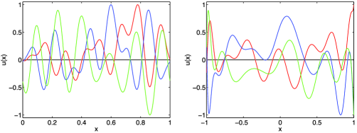
Figure 1: Sample functions from a random sum of the form $u(x,\omega)=\sum_{k=0}^{N}g_{k}(\omega)\varphi_{k}(x)$ where $g_{1},\ldots,g_{N}$ are independent standard Gaussian random variables. In the left diagram, we consider random periodic functions, that is, the basis functions $\varphi_{k}$ are given by $\varphi_{2k}(x)=\break\cos(2\pi kx)$ and $\varphi_{2k-1}(x)=\sin(2\pi kx)$, in the right diagram they are the Chebyshev polynomials $\varphi_{k}(x)=\cos(k\arccos x)$. In each case, we choose $N=16$.

The more serious restriction in mischaikowwanner07a is the use of periodic random fields, which due to the fact that the associated spatial correlation function is homogeneous, simplifies many of the estimates. In general, however, one expects to encounter nonhomogeneous random fields. In such cases, it seems unreasonable to expect that uniform sampling provides the optimal choice. For example, in Figure 1, three sample functions each are shown for a random sum involving periodic basis functions and Chebyshev polynomials. As one would expect, the zeros of the random Chebyshev sum are more closely spaced at the boundary, and therefore small uniform discretization are most likely not optimal for determining the topology of the nodal domains.

With this as motivation, we allow for a more general sampling technique. We remark that because of the subtlety of some of the necessary estimates we restrict our attention in this paper to one-dimensional domains.

Definition 1.1 ((Nonuniform approximation of generalized nodal domains)).

Consider a compact interval $[a,b]\subset\mathbb{R}$, a threshold function $\mu\dvtx[a,b]\to\mathbb{R}$, and a function $u\dvtx[a,b]\to\mathbb{R}$. Then we define the generalized nodal domains of $u$ by

$$N_{\mu}^{\pm}=\bigl{\{}x\in[a,b]\dvtx\pm\bigl{(}u(x)-\mu(x)\bigr{)}\geq 0\bigr{\}},$$ (1)

which for the case of $\mu(x)\equiv 0$ reduces to the classical definition of a nodal domain in couranthilbert53a . An $M$-discretization of $[a,b]$ is a collection of $M+1$ grid points

$$a=x_{0}<x_{1}<\cdots<x_{M}=b,$$

and we define $x_{M+1}=x_{M}=b$ in the following. The cubical approximations $Q_{M}^{\pm}$ of the generalized nodal domains $N_{\mu}^{\pm}$ of $u$ are defined as the sets

$$Q_{\mu,M}^{\pm}:=\bigcup\bigl{\{}[x_{k},x_{k+1}]\dvtx\pm\bigl{(}(u-\mu)(x_{k})\bigr{)}\geq 0,k=0,\ldots,M\bigr{\}}.$$

Given a subset $X\subset[a,b]$, let $\beta_{0}(X)$ denote the number of components of $X$. Consider a random field $u\dvtx[a,b]\times\Omega\to\mathbb{R}$ over the probability space $(\Omega,\mathcal{F},\mathbb{P})$. We are interested in optimally characterizing the topology, that is, determining the number of components, of the nodal domains $N_{\mu}^{\pm}$ in terms of the cubical approximations $Q_{\mu,M}^{\pm}$. In other words, our goal is to choose the $M$-discretization of $[a,b]$ in such a way as to optimize

$$\mathbb{P}\{\beta_{0}(N_{\mu}^{\pm})=\beta_{0}(Q_{\mu,M}^{\pm})\}.$$

We provide two results addressing this question. The first characterizes the choice of the sampling points $a=x_{0}<x_{1}<\cdots<x_{M}=b$ under reasonably general abstract conditions. More precisely, consider the following assumptions:

1. [(A3)]

2. For every $x\in[a,b]$, we have $\mathbb{P}\{u(x)=\mu(x)\}=0$.

3. The random field is such that $\mathbb{P}\{u-\mu\mbox{ has a double zero in }[a,b]\}=0$.

4. For $\sigma\in\{\pm 1\}$, $x\in[a,b]$ and $\delta>0$ with $x+\delta\in[a,b]$ define

   $$p_{\sigma}(x,\delta) = \mathbb{P}\biggl{\{}\sigma u(x)\geq\sigma\mu(x),\sigma u\biggl{(}x+\frac{\delta}{2}\biggr{)}\leq\sigma\mu\biggl{(}x+\frac{\delta}{2}\biggr{)},$$

   $$\hskip 107.0pt\sigma u(x+\delta)\geq\sigma\mu(x+\delta)\biggr{\}}.$$

   Then there exists a continuously differentiable function $\mathcal{C}_{0}\dvtx[a,b]\to\mathbb{R}^{+}$ as well as a constant $\mathcal{C}_{1}>0$ such that for all $x\in[a,b]$ with $x+\delta\in[a,b]$ we have

   $$p_{+1}(x,\delta)+p_{-1}(x,\delta)\leq\mathcal{C}_{0}(x)\cdot\delta^{3}+\mathcal{C}_{1}\cdot\delta^{4}.$$

In Section 3, we prove the following result.

Theorem 1.2 ((Sampling based on local probabilities)).

Consider a probability space $(\Omega,\mathcal{F},\mathbb{P})$, a continuous threshold function $\mu\dvtx[a,b]\to\mathbb{R}$, and a random field $u\dvtx[a,b]\times\Omega\to\mathbb{R}$ over $(\Omega,\mathcal{F},\mathbb{P})$ such that for $\mathbb{P}$-almost all $\omega\in\Omega$ the function $u(\cdot,\omega)\dvtx[a,b]\to\mathbb{R}$ is continuous. Choose the sampling points $a=x_{0}<\cdots<x_{M}=b$ such that

$$\int_{x_{k-1}}^{x_{k}}\sqrt[3]{\mathcal{C}_{0}(x)}\,dx=\frac{1}{M}\cdot\int_{a}^{b}\sqrt[3]{\mathcal{C}_{0}(x)}\,dx\qquad\mbox{for all }k=1,\ldots,M,$$

and consider the generalized nodal domains $N_{\mu}^{\pm}(\omega)$ and their approximations $Q_{\mu,M}^{\pm}(\omega)$ as in Definition 1.1. If assumptions (A1), (A2) and (A3) hold, then

$$\mathbb{P}\{\beta_{0}(N_{\mu}^{\pm})=\beta_{0}(Q_{\mu,M}^{\pm})\}\geq 1-\frac{4}{3M^{2}}\cdot\biggl{(}\int_{a}^{b}\sqrt[3]{\mathcal{C}_{0}(x)}\,dx\biggr{)}^{3}+O\biggl{(}\frac{1}{M^{3}}\biggr{)}.$$ (2)

This theorem is a direct generalization of the corresponding result in (mischaikowwanner07a , Theorem 1.3). Numerical computations presented in Section 2 suggest that for certain nonhomogeneous random fields this estimate is sharp—and in fact an enormous improvement over the homogeneous result where $\mathcal{C}_{0}(x)$ is replaced by $\max_{x\in G}\mathcal{C}_{0}(x)$.

Of course in practice one is interested in applying Theorem 1.2 to specific random fields. This requires the verification of assumptions (A1), (A2) and (A3), preferably in terms of central random field characteristics.

Definition 1.3.

For a random field $u\dvtx[a,b]\times\Omega\to\mathbb{R}$ over a probability space $(\Omega,\mathcal{F},\mathbb{P})$, we define its spatial correlation function $R\dvtx[a,b]^{2}\to\mathbb{R}$ as

$$R(x,y)=\mathbb{E}\bigl{(}\bigl{(}u(x)-\mathbb{E}u(x)\bigr{)}\bigl{(}u(y)-\mathbb{E}u(y)\bigr{)}\bigr{)}\qquad\mbox{for all }x,y\in[a,b],$$

where $\mathbb{E}$ denotes the expected value of a random variable over $(\Omega,\mathcal{F},\mathbb{P})$.

If the random field is sufficiently smooth, then the derivatives of the spatial correlation function,

$$R_{k,\ell}(x)=\frac{\partial^{k+\ell}R}{\partial x^{k}\,\partial y^{\ell}}(x,x),$$ (3)

have a natural interpretation in terms of spatial derivatives of the random field $u$. Since

$$R_{k,\ell}(x)={\mathbb{E}}\bigl{(}\bigl{(}u^{(k)}(x)-\mathbb{E}u^{(k)}(x)\bigr{)}\bigl{(}u^{(\ell)}(y)-\mathbb{E}u^{(\ell)}(y)\bigr{)}\bigr{)},$$

the function $R_{k,k}$ contains averaged information on the square of the $k$th derivative of the random function $u$, more precisely, its variance.

To relate the spatial correlation function to the function $\mathcal{C}_{0}$ in Theorem 1.2, we specialize to Gaussian random fields. To be more precise, we make the following assumptions.

1. [(G2)]

2. Consider a Gaussian random field $u\dvtx[a,b]\times\Omega\to\mathbb{R}$ over a probability space $(\Omega,\mathcal{F},\mathbb{P})$ such that $u(\cdot,\omega)\dvtx[a,b]\to\mathbb{R}$ is twice continuously differentiable for $\mathbb{P}$-almost all $\omega\in\Omega$. Furthermore, assume that for every $x\in[a,b]$ the expected value of $u(x)$ satisfies

   $$\mathbb{E}u(x)=0.$$

3. The spatial correlation function $R$ is three times continuously differentiable in a neighborhood of the diagonal $x=y$ and the matrix

   $$\mathcal{R}(x)=\pmatrix{R_{0,0}(x)&R_{1,0}(x)&R_{2,0}(x)\vspace*{2pt}\cr R_{1,0}(x)&R_{1,1}(x)&R_{2,1}(x)\vspace*{2pt}\cr R_{2,0}(x)&R_{2,1}(x)&R_{2,2}(x)}$$ (4)

   is positive definite for all $x\in[a,b]$.

We make considerable use of $\mathcal{R}$, and thus introduce the following notation

$$\mathcal{R}_{33}^{m} := R_{0,0}R_{1,1}-R_{1,0}^{2},$$

$$\mathcal{R}_{32}^{m} := R_{0,0}R_{2,1}-R_{1,0}R_{2,0},$$ (5)

$$\mathcal{R}_{31}^{m} := R_{1,0}R_{2,1}-R_{1,1}R_{2,0}.$$

These expressions are just the determinants of minors of $\mathcal{R}$. This allows us to state the following theorem.

Theorem 1.4 ((Sampling based on spatial correlation)).

Consider a Gaussian random field $u\dvtx[a,b]\times\Omega\to\mathbb{R}$ satisfying (G1) and (G2), and a threshold function $\mu\dvtx[a,b]\to\mathbb{R}$ of class $C^{3}$. Choose the sampling points $a=x_{0}<\cdots<x_{M}=b$ in such a way that

$$\int_{x_{k-1}}^{x_{k}}\sqrt[3]{\mathcal{C}(x)}\,dx=\frac{1}{M}\cdot\int_{a}^{b}\sqrt[3]{\mathcal{C}(x)}\,dx\qquad\mbox{for all }k=1,\ldots,M,$$

where

$$\mathcal{C}(x)=\frac{\det\mathcal{R}(x)}{48\pi\mathcal{R}_{3,3}^{m}(x)^{3/2}}\cdot\bigl{(}1+\mathcal{A}(x)\bigr{)}\cdot e^{-\mathcal{B}(x)},$$ (6)

given

$$\mathcal{A}(x) = \frac{(\mathcal{R}_{3,1}^{m}(x)\mu(x)-\mathcal{R}_{3,2}^{m}(x)\mu^{\prime}(x)+\mathcal{R}_{3,3}^{m}(x)\mu^{\prime\prime}(x))^{2}}{\mathcal{R}_{3,3}^{m}(x)\det\mathcal{R}(x)}\geq 0,$$

$$\mathcal{B}(x) = \frac{(R_{1,0}(x)\mu(x)-R_{0,0}(x)\mu^{\prime}(x))^{2}+\mathcal{R}_{3,3}^{m}(x)\mu(x)^{2}}{2R_{0,0}(x)\mathcal{R}_{3,3}^{m}(x)}\geq 0.$$

Let $Q_{\mu,M}^{\pm}(\omega)$ denote the cubical approximations of the random generalized nodal domains $N_{\mu}^{\pm}(\omega)$ of $u(\cdot,\omega)$. Then

$$\mathbb{P}\{\beta_{0}(N_{\mu}^{\pm})=\beta_{0}(Q_{\mu,M}^{\pm})\}\geq 1-\frac{1}{M^{2}}\cdot\biggl{(}\int_{a}^{b}\sqrt[3]{\mathcal{C}(x)}\,dx\biggr{)}^{3}+O\biggl{(}\frac{1}{M^{3}}\biggr{)}.$$ (7)

The proof of Theorem 1.4 is presented in Section 5. However, it depends on nontrivial results concerning the asymptotic behavior of sign-distribution probabilities of parameter-dependent Gaussian random variables. These results are developed in Section 4.

The number of nodal domains $\beta_{0}(N_{\mu}^{\pm})$ is clearly dependent upon the zeros of $u-\mu$. Thus, it is reasonable to expect that there is some relationship between the function $\mathcal{C}$ derived in Theorem 1.4 and the density of the zeros of the random field $u$. The first step is to obtain a density function. For this, a weaker form of (G2) is sufficient.

1. [(G3)]

2. Assume that the spatial correlation function $R$ is two times continuously differentiable in a neighborhood of the diagonal $x=y$ and that $R(x,x)>0$ for all $x\in[a,b]$.

Finding the density of the zeros of random fields has been studied in a variety of settings, see, for example, adlertaylor07a , bharuchareids86a , cramerleadbetter04a , edelmankostlan95a , farahmand98a , as well as the references therein. The following theorem can be found in cramerleadbetter04a , (13.2.1), page 285.

Theorem 1.5 ((Density of zeros of a random field)).

Consider a Gaussian random field $u\dvtx[a,b]\times\Omega\to\mathbb{R}$ satisfying (G1) and (G3). Then the density function for the number of zeros of $u$ is given by

$$\mathcal{D}(x)=\frac{\mathcal{R}_{3,3}^{m}(x)^{1/2}}{\pi\cdot R_{0,0}(x)}.$$ (8)

In other words, for every interval $I\subset[a,b]$ the expected number of zeros of $u$ in $I$ is given by $\int_{I}\mathcal{D}(x)\,dx$.

While Theorem 1.5 has been known for quite some time, its implications are surprising. As is demonstrated through examples in Section 2 there is no simple discernible relationship between the function $\mathcal{C}^{1/3}$ of Theorem 1.4 and the density function $\mathcal{D}$.

As is made clear at the beginning of this Introduction, our motivation is to develop optimal sampling methods for the analysis of complicated time-dependent patterns. Thus, before turning to the proofs of the above-mentioned results, we begin, in Section 2, with demonstrations of possible applications and implications of Theorem 1.4. In particular, we consider several random generalized Fourier series $u\dvtx[a,b]\times\Omega\to\mathbb{R}$ defined by

$$u(x,\omega)=\sum_{k=0}^{\infty}g_{k}(\omega)\cdot\varphi_{k}(x),$$ (9)

where $\varphi_{k}\dvtx[a,b]\to\mathbb{R}$, $k\in\mathbb{N}_{0}$, denotes a family of smooth functions and we assume that the Gaussian random variables $g_{k}\dvtx\Omega\to\mathbb{R}$, $k\in\mathbb{N}_{0}$, are defined over a common probability space $(\Omega,\mathcal{F},\mathbb{P})$ with mean $0$.

We conclude the paper with a general discussion of future work concerning natural generalizations to higher dimensions.

2 Sampling of specific random sums

To demonstrate the applicability and implications of Theorem 1.4, we consider in this section several random generalized Fourier series $u\dvtx[a,b]\times\Omega\to\mathbb{R}$ of the form in (9). As mentioned before, the functions $\varphi_{k}\dvtx[a,b]\to\mathbb{R}$, $k\in\mathbb{N}_{0}$, denote a family of smooth functions and we assume that the random variables $g_{k}\dvtx\Omega\to\mathbb{R}$, $k\in\mathbb{N}_{0}$, are Gaussian with vanishing mean, and defined over a common probability space $(\Omega,\mathcal{F},\mathbb{P})$. We would like to point out that these random variables do not need to be independent, and we define

$$\alpha_{k,m}=\mathbb{E}(g_{k}g_{m})\qquad\mbox{for all }k,m\in\mathbb{N}_{0}.$$

Then one can easily show that

$$R_{k,\ell}(x)={\mathbb{E}}\bigl{(}u^{(k)}(x)u^{(\ell)}(x)\bigr{)}=\sum_{i,j=0}^{\infty}\alpha_{i,j}\varphi_{i}^{(k)}(x)\varphi_{j}^{(\ell)}(x).$$

If in addition the random variables $g_{k}$ are pairwise independent, then we have

$$R_{k,\ell}(x)=\sum_{j=0}^{\infty}\alpha_{j,j}\varphi_{j}^{(k)}(x)\varphi_{j}^{(\ell)}(x),$$

where $\alpha_{j,j}\geq 0$ for all $j\in\mathbb{N}_{0}$. One can show that this diagonalization can always be achieved for Gaussian random fields, provided the basis functions $\varphi_{k}$ are chosen appropriately. For more details, we refer the reader to adlertaylor07a , Theorems 3.1.1 and 3.1.2, Lemma 3.1.4.

Within the above framework of random generalized Fourier series, we specifically consider several classes:

• Random Chebyshev polynomials $u\dvtx[-1,1]\times\Omega\to\mathbb{R}$ of the form

  $$u(x,\omega)=\sum_{k=0}^{N}g_{k}(\omega)\cdot\cos(k\arccos x)\qquad\mbox{with }\mathbb{E}(g_{k}g_{\ell})=\delta_{k,\ell}.$$ (10)

• Random cosine series $u\dvtx[0,1]\times\Omega\to\mathbb{R}$ of the form

  $$u(x,\omega)=\sum_{k=0}^{N}g_{k}(\omega)\cdot\cos(k\pi x)\qquad\mbox{with }\mathbb{E}(g_{k}g_{\ell})=\delta_{k,\ell}.$$ (11)

• Random $L$-periodic functions $u\dvtx\mathbb{R}\times\Omega\to\mathbb{R}$ of the form

  $$u(x,\omega) = \sum_{k=0}^{\infty}a_{k}\cdot\biggl{(}g_{2k}(\omega)\cdot\cos\frac{2\pi kx}{L}+g_{2k-1}(\omega)\cdot\sin\frac{2\pi kx}{L}\biggr{)}$$

  $$\eqntext{\mbox{with }\mathbb{E}(g_{k}g_{\ell})=\delta_{k,\ell},}$$ (13)

  with real constants $a_{k}$.

• Random polynomials $u\dvtx[-3,3]\times\Omega\to\mathbb{R}$ with Gaussian coefficients of binomial variance of the form

  $$u(x,\omega)=\sum_{k=0}^{N}g_{k}(\omega)\cdot x^{k}\qquad\mbox{with }\mathbb{E}(g_{k}g_{\ell})=\delta_{k,\ell}\cdot\pmatrix{N\cr k},$$ (14)

• Random polynomials $u\dvtx[-3,3]\times\Omega\to\mathbb{R}$ with Gaussian coefficients of unit variance of the form

  $$u(x,\omega)=\sum_{k=0}^{N}g_{k}(\omega)\cdot x^{k}\qquad\mbox{with }\mathbb{E}(g_{k}g_{\ell})=\delta_{k,\ell}.$$ (15)

As is indicated in Section 1, we assume that all the random coefficients are centered Gaussian random variables over a common probability space $(\Omega,\mathcal{F},\mathbb{P})$.

2.1 The case of vanishing threshold function

We begin our applications by thresholding sample random sums at their expected value, that is, we use the threshold function $\mu\equiv 0$. In this particular case, the function $\mathcal{C}(x)$ defined by (6) in Theorem 1.4 simplifies to

$$\mathcal{C}(x)=\frac{\det\mathcal{R}(x)}{48\pi\mathcal{R}_{3,3}^{m}(x)^{3/2}},$$ (16)

since both $\mathcal{A}(x)$ and $\mathcal{B}(x)$ vanish.

For the case of random Chebyshev polynomials (10), the left diagram in Figure 2 shows three normalized sample functions

$$\frac{\mathcal{C}^{1/3}(x)}{\int_{-1}^{1}\mathcal{C}^{1/3}(x)\,dx}$$

for $N=3,5,10$. The right diagram shows the expected number of zeros of the random Chebyshev polynomials as a function of $N$ (red curve), which grows proportional to $N$. Thus, in order to sample the random field sufficiently fine, we expect to use significantly more than $O(N)$ discretization points. The blue curve in the right diagram of Figure 2 shows the values of $M$ for which the bound in (7) of Theorem 1.4 implies a correctness probability of $95\%$, and a least squares fit of this curve furnishes $M\sim N^{3/2}$. For comparison, the green curve in the same diagram shows the values of $M$ for which the bound in our previous result (mischaikowwanner07a , Theorem 1.4) implies a correctness probability of $95\%$, provided we apply this theorem with $\mathcal{C}_{0}$ given as the $\max_{x\in[-1,1]}\mathcal{C}_{0}(x)$. Notice that in this case we have $M\sim N^{3}$. In other words, only the topology-guided sampling result of the current paper yields a reasonable growth for the number of sampling points. In fact, based on our results for periodic random fields in mischaikowwanner07a and the numerical simulations in dayetal07a , we expect that $M\sim N^{3/2}$ is the optimal discretization size.

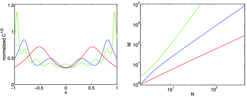
Figure 2: Topology-guided sampling of random Chebyshev polynomials (10). The left diagram shows the functions $\mathcal{C}^{1/3}$ for $N=3,5,10$ (red, blue and green, respectively—increasing values of $N$ increase the number of extrema); for comparison reasons, each curve has been scaled in such a way that the area under the graph is one. The right diagram shows the expected number of zeros of the random Chebyshev polynomials as a function of $N$ (bottom red curve), the value of $M$ for which Theorem 1.4 gives a correctness probability of $95\%$ (middle blue curve), and the value of $M$ for which mischaikowwanner07a gives a correctness probability of $95\%$ (top green curve) with $\mathcal{C}_{0}=\max\mathcal{C}_{0}(x)$.

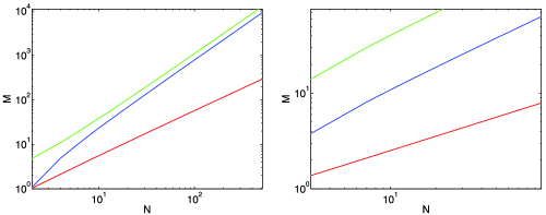
Figure 3: Topology-guided sampling of random trigonometric polynomials (11) satisfying Neumann boundary conditions (left diagram) and random algebraic polynomials (14) with binomial variances (right diagram). The curves show the expected numbers of zeros (bottom red curve), the discretization size required by Theorem 1.4 to achieve $95\%$ correctness (middle blue curve), and the discretization size required by mischaikowwanner07a for a correctness probability of $95\%$ (top green curve), with $\mathcal{C}_{0}=\max\mathcal{C}_{0}(x)$.

For the case of random cosine sums (11), that is, random trigonometric sums satisfying homogeneous Neumann boundary conditions, the analogue of the right diagram in Figure 2 is depicted in the left diagram of Figure 3. Notice that for the random cosine sums the expected number of zeros is proportional to $N$, and the required number of sampling points has to be proportional to $N^{3/2}$ for both Theorem 1.4 and mischaikowwanner07a , Theorem 1.4. In other words, in this situation the gains from topology-guided sampling are no longer as large as in the context of Chebyshev polynomials. Also in this case, the curves for $M$ are obtained in such a way that the right-hand side in (7) or the corresponding bound in mischaikowwanner07a equals $95\%$

Similar behavior can be seen in the case of random polynomials (14) with Gaussian coefficients of binomial variance; see the right diagram of Figure 3. For the random algebraic polynomials (14), one can show that the expected number of zeros is proportional to $N^{1/2}$, and the required number of sampling points implied by (7) or mischaikowwanner07a has to be proportional to $N^{3/4}$ for both results. In fact, the function $\mathcal{C}$ can be computed explicitly in this case. Due to (14), the spatial correlation function $R$ is given by

$$R(x,y)=\sum_{k=0}^{N}{N\choose k}x^{k}y^{k}=(1+xy)^{N},$$

which after some elementary computations furnishes

$$\mathcal{C}(x)=\frac{N^{1/2}(N-1)}{24\pi(1+x^{2})^{3}}.$$ (17)

As for the case of random polynomials with Gaussian coefficients of unit variance, a classical result due to Kac kac43a , kac49a implies that the expected number of zeros is proportional to $\log N$. In this case, Theorem 1.4 implies that the required number of sampling points has to be proportional to $(\log N)^{3/2}$.

2.2 The case of constant threshold function

We now turn our attention to a constant threshold function $\mu(x)=\tau$, for some real number $\tau$. In this case, the function $\mathcal{C}(x)$ in Theorem 1.4 simplifies to

$$\mathcal{C}(x)=\frac{\det\mathcal{R}(x)}{48\pi\mathcal{R}_{3,3}^{m}(x)^{3/2}}\cdot\mathcal{S}(x),$$ (18)

where

$$\mathcal{S}(x)=\biggl{(}1+\frac{\mathcal{R}_{3,1}^{m}(x)^{2}\tau^{2}}{\mathcal{R}_{3,3}^{m}(x)\det\mathcal{R}(x)}\biggr{)}\cdot\exp\biggl{(}-\frac{R_{1,0}(x)^{2}+\mathcal{R}_{3,3}^{m}(x)}{2R_{0,0}(x)\mathcal{R}_{3,3}^{m}(x)}\cdot\tau^{2}\biggr{)}.$$ (19)

For large values of $|\tau|$, the scaling function $\mathcal{S}(x)$ will be close to zero, and it therefore effectively decreases the probability for mistakes in the homology computation. In fact, it decreases exponentially fast with respect to $|\tau|$. However, as is shown in Figure 4 for the random Chebyshev polynomials (10), for values of $\tau$ close to zero, there can be regions in which the probability for mistakes actually increases. This behavior is even more pronounced in the case of random algebraic polynomials (14) and (15), which is shown in Figure 5.

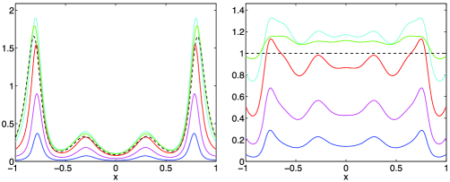
Figure 4: Effect of varying the threshold $\tau$ on the function $\mathcal{C}(x)$ in (18) for random Chebyshev polynomials (10) with $N=5$. The left diagram shows the function $\mathcal{C}(x)$ for $\tau=0,1,2,3,4,5$ (black, green, cyan, red, magenta, blue), the right diagram shows only the function $\mathcal{S}(x)$ defined in (19).

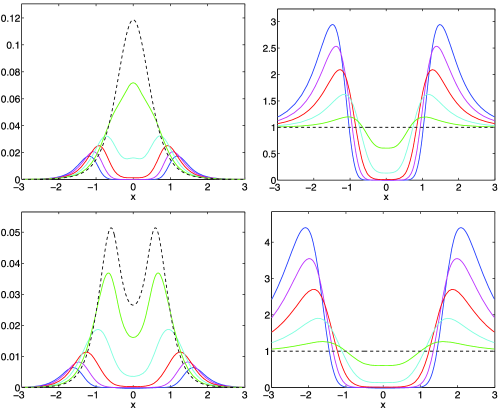
Figure 5: Effect of varying the threshold $\tau$ on the function $\mathcal{C}(x)$ in (18) for random algebraic polynomials (14) (top row) and (15) (bottom row) with $N=5$. In each row, the left diagram shows $\mathcal{C}(x)$ for $\tau=0,1,2,3,4,5$ (black, green, cyan, red, magenta, blue), and the right diagram shows only the function $\mathcal{S}(x)$ defined in (19).

2.3 The case of varying threshold function

We now consider the case of a general threshold function under the following assumptions. Suppose a deterministic function $\mu(x)$ is perturbed by a centered Gaussian random field $u(x,\omega)$, and that we are interested in determining the classical nodal domains of the sum

$$v(x,\omega)=\mu(x)+u(x,\omega).$$

Sampling $v(x,\omega)$ at the threshold zero is obviously equivalent to sampling $u(x,\omega)$ at the threshold $-\mu(x)$. Thus, we can use Theorem 1.4 to find the optimal location of the sampling points using the function $\mathcal{C}(x)$ defined in (6).

In order to demonstrate the effects of the varying threshold function $-\mu(x)$ more clearly, we now assume that the perturbing random field $u$ is homogeneous, that is, we assume that $u$ is a random $L$-periodic function of the form (• ‣ 2). Furthermore, we assume that the real scaling factors $a_{k}$ in (• ‣ 2) satisfy

$$\sum_{k=0}^{\infty}k^{6}a_{k}^{2}<\infty,$$

and that at least two of the $a_{k}$ do not vanish. It was shown in mischaikowwanner07a that in this case the spatial correlation function $R$ is given by

$$R(x,y)=\mathbb{E}u(x)u(y)=\sum_{k=0}^{\infty}a_{k}^{2}\cdot\cos\frac{2\pi k(x-y)}{L}.$$

From this, one can readily see that the matrix function $\mathcal{R}(x)$ defined in (4) is constant and given by

$$\mathcal{R}(x)=\pmatrix{A_{0}&0&-\dfrac{4\pi^{2}A_{1}}{L^{2}}\vspace*{2pt}\cr 0&\dfrac{4\pi^{2}A_{1}}{L^{2}}&0\vspace*{2pt}\cr-\dfrac{4\pi^{2}A_{1}}{L^{2}}&0&\dfrac{16\pi^{4}A_{2}}{L^{4}}},$$

where

$$A_{\ell}=\sum_{k=0}^{\infty}k^{2\ell}a_{k}^{2}.$$

Thus, the function $\mathcal{C}(x)$ in (6) is now given as

$$\mathcal{C}(x)=\frac{\pi^{2}}{6L^{3}}\cdot\frac{A_{0}A_{2}-A_{1}^{2}}{A_{0}^{3/2}A_{1}^{1/2}}\cdot\mathcal{S}(x),$$ (20)

where

$$\mathcal{S}(x) = \biggl{(}1+\frac{(A_{1}\mu(x)+A_{0}\mu^{\prime\prime}(x)\cdot({L^{2}}/{(4\pi^{2})}))^{2}}{A_{0}(A_{0}A_{2}-A_{1}^{2})}\biggr{)}$$

$${}\times\exp\biggl{(}-\frac{A_{1}\mu(x)^{2}+A_{0}\mu^{\prime}(x)^{2}\cdot({L^{2}}/{(4\pi^{2})})}{2A_{0}A_{1}}\biggr{)}.$$

Notice that the exponential factor is bounded above by $\exp(-\mu(x)^{2}/(2A_{0}))$, that is, large function values of $\mu(x)$ lead to small failure probabilities.

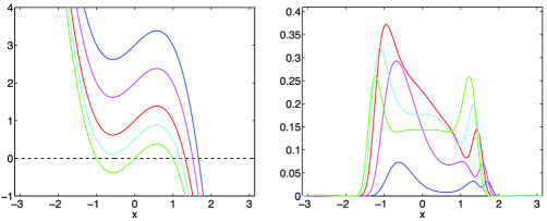
Figure 6: Sampling of deterministic functions $\mu(x)$ perturbed by homogeneous random noise. The left image shows the functions $\mu(x)=x-x^{3}+\tau$ for $\tau=0,0.5,1,2,3$ (green, cyan, red, magenta, blue), the right images shows the corresponding functions $\mathcal{C}(x)$ defined in (20).

We close this subsection by visualizing the function $\mathcal{C}(x)$ defined in (20) for the deterministic function $\mu(x)=x-x^{3}+\tau$ and $\tau$-values between $0$ and $3$. The specific functions $\mu(x)$ are shown in the left image of Figure 6. In the right image, the corresponding functions $\mathcal{C}(x)$ are shown, where $u$ is defined as in (• ‣ 2) with $a_{k}=0$ for $k=0$ and $k>N$, as well as $a_{k}=N^{-1/2}$ for $k=1,\ldots,N$. This implies that the variance of $u(x)$ equals $1$. In Figure 6, we use $N=5$.

2.4 Comparison with density-guided sampling

In order to illustrate the differences between the density of zeros $\mathcal{D}$ derived in Theorem 1.5 and the function $\mathcal{C}^{1/3}$ from Theorem 1.4, we return to our examples from the last section. For each of these examples, Figure 7 depicts both

$$\frac{\mathcal{C}^{1/3}(x)}{\int\mathcal{C}^{1/3}(x)\,dx}\quad\mbox{and}\quad\frac{\mathcal{D}(x)}{\int\mathcal{D}(x)\,dx}$$

for the case $N=5$. It is evident from these graphs that in most cases, the homology-based sampling density is different from the actual density of zeros. In fact, in many cases it behaves anticyclic to $\mathcal{D}$ in the sense that the local extrema of $\mathcal{C}^{1/3}$ alternate with the local extrema of $\mathcal{D}$.

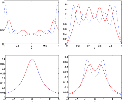
Figure 7: A comparison of the function $\mathcal{C}^{1/3}$ and the density function $\mathcal{D}$ for random Chebyshev polynomials (10) (top left diagram), random trigonometric polynomials (11) (top right), random algebraic polynomials (14) (bottom left), and random algebraic polynomials (15) (bottom right). In all cases, the areas under the graphs have been normalized to one, and we chose $N=5$.

There are, however, exceptions, as the case of the random algebraic polynomial (14) demonstrates. In this case, it follows from Theorem 1.5 that

$$\mathcal{D}(x)=\frac{N^{1/2}}{\pi(1+x^{2})},$$

and together with (17) this shows that the normalized $\mathcal{C}^{1/3}$- and $\mathcal{D}$-functions coincide.

3 Sampling based on local probabilities

The goal of this section is the proof of Theorem 1.2, which is a generalization of mischaikowwanner07a , Theorem 1.3. Thus, we begin by recalling some basic definitions and results.

As is indicated in Section 1, given a continuous function $u\dvtx[a,b]\to\mathbb{R}$ and a continuous threshold $\mu\dvtx[a,b]\to\mathbb{R}$ we are interested in determining the number of components of the generalized nodal domain $N_{\mu}^{\pm}$ in terms of a cubical approximation $Q_{\mu,M}^{\pm}$ obtained via sampling at $M+1$ points as described in Definition 1.1. For suitably chosen discretization points, and under appropriate regularity and nondegeneracy conditions on $u$ one can then expect that the number of components of $Q_{\mu,M}^{\pm}$ and $N_{\mu}^{\pm}$ agree. One only has to be able to verify that the function $u$ has at most one zero (counting multiplicity) in each of the intervals $[x_{k-1},x_{k}]$, for $k=1,\ldots,M$. This is accomplished using the following framework which goes back to Dunnage dunnage66a .

Definition 3.1.

A continuous function $u\dvtx[a,b]\to\mathbb{R}$ has a double crossover on the interval $[\alpha,\beta]\subset[a,b]$, if

$$\sigma\cdot u(\alpha)\geq 0,\qquad\sigma\cdot u\biggl{(}\frac{\alpha+\beta}{2}\biggr{)}\leq 0\quad\mbox{and}\quad\sigma\cdot u(\beta)\geq 0$$ (21)

for one choice of the sign $\sigma\in\{\pm 1\}$.

Definition 3.2.

Let $u\dvtx[a,b]\to\mathbb{R}$ be a continuous function.

• The dyadic points in the interval $[\alpha,\beta]$ are defined as

  $$d_{n,k}=\alpha+(\beta-\alpha)\cdot\frac{k}{2^{n}}\qquad\mbox{for all }k=0,\ldots,2^{n}\mbox{ and }n\in\mathbb{N}_{0}.$$

  The dyadic subintervals of $[\alpha,\beta]$ are the intervals $[d_{n,k},d_{n,k+1}]$ for all $k=0,\ldots,2^{n}-1$ and $n\in\mathbb{N}_{0}$.

• The interval $[\alpha,\beta]\subset[a,b]$ is admissible for $u$, if the function $u$ does not have a double crossover on any of the dyadic subintervals of $[\alpha,\beta]$.

It was shown in mischaikowwanner07a that the concept of admissibility implies the suitability of our nodal domain approximations. More precisely, the following is a slight rewording of mischaikowwanner07a , Proposition 2.5.

Proposition 3.3 ((Validation criterion)).

Let $u\dvtx[a,b]\to\mathbb{R}$ be a continuous function and let $\mu\dvtx[a,b]\to\mathbb{R}$ be a continuous threshold function. Let $N_{\mu}^{\pm}$ denote the generalized nodal domains of $u$, and let $Q_{\mu,M}^{\pm}$ denote their cubical approximations as in Definition 1.1. Furthermore, assume that the following hold:

1. [(c)]

2. The function $u-\mu$ is nonzero at all grid points $x_{k}$, for $k=0,\ldots,M$.

3. The function $u-\mu$ has no double zero in $(a,b)$, that is, if $x\in(a,b)$ is a zero of $u$, then $u-\mu$ attains both positive and negative function values in every neighborhood of $x$.

4. For every $k=1,\ldots,M$, the interval $[x_{k-1},x_{k}]$ between consecutive discretization points is admissible for $u-\mu$ in the sense of Definition 3.2.

Then we have

$$\beta_{0}(N_{\mu}^{\pm})=\beta_{0}(Q_{\mu,M}^{\pm}).$$

The following lemma provides bounds on the probability for admissibility of a given interval.

Lemma 3.4.

Consider a probability space $(\Omega,\mathcal{F},\mathbb{P})$, a continuous threshold function $\mu\dvtx[a,b]\to\mathbb{R}$, and a random field $u\dvtx[a,b]\times\Omega\to\mathbb{R}$ over $(\Omega,\mathcal{F},\mathbb{P})$ such that $u(\cdot,\omega)$ is continuous for $\mathbb{P}$-almost all $\omega\in\Omega$. In addition, assume that (A1), (A2) and (A3) hold. If $[x,x+\delta]\subset[a,b]$, then

$$\mathbb{P}([x,x+\delta]\mbox{ is not admissible for }u-\mu)$$

(22)

$$\qquad\leq\frac{4\mathcal{C}_{0}(x)}{3}\cdot\delta^{3}+\biggl{(}\frac{4L}{3}+\frac{8\mathcal{C}_{1}}{7}\biggr{)}\cdot\delta^{4},$$

where $L=\max\{|\mathcal{C}_{0}^{\prime}(y)|\dvtx y\in[a,b]\}$.

If the interval $I=[x,x+\delta]$ is not admissible, then the function $u-\mu$ has a double crossover on one of its dyadic subintervals. If we now denote the dyadic points in $I$ by $d_{n,k}$ as in Definition 3.2, then together with (A3) one obtains the estimate

$$\mathbb{P}\{I\mbox{ is not admissible}\} \leq \sum_{n=0}^{\infty}\sum_{k=0}^{2^{n}-1}\bigl{(}p_{+1}(d_{n,k},\delta/2^{n})+p_{-1}(d_{n,k},\delta/2^{n})\bigr{)}$$

$$\leq \sum_{n=0}^{\infty}\sum_{k=0}^{2^{n}-1}\biggl{(}\mathcal{C}_{0}(d_{n,k})\cdot\biggl{(}\frac{\delta}{2^{n}}\biggr{)}^{3}+\mathcal{C}_{1}\cdot\biggl{(}\frac{\delta}{2^{n}}\biggr{)}^{4}\biggr{)}.$$

Since $\mathcal{C}_{0}$ is continuously differentiable, we can define $L=\max\{|\mathcal{C}_{0}^{\prime}(y)|\dvtx y\in[a,b]\}$, and the definition of the dyadic points implies

$$\mathcal{C}_{0}(d_{n,k})\leq\mathcal{C}_{0}(x)+L\cdot(d_{n,k}-x)\leq\mathcal{C}_{0}(x)+L\delta.$$

This finally furnishes

$$\mathbb{P}\{I\mbox{ is not admissible}\} \leq \sum_{n=0}^{\infty}\sum_{k=0}^{2^{n}-1}\biggl{(}\bigl{(}\mathcal{C}_{0}(x)+L\delta\bigr{)}\cdot\biggl{(}\frac{\delta}{2^{n}}\biggr{)}^{3}+\mathcal{C}_{1}\cdot\biggl{(}\frac{\delta}{2^{n}}\biggr{)}^{4}\biggr{)}$$

$$= \frac{4\mathcal{C}_{0}(x)}{3}\cdot\delta^{3}+\biggl{(}\frac{4L}{3}+\frac{8\mathcal{C}_{1}}{7}\biggr{)}\cdot\delta^{4}.$$

Combining Proposition 3.3, Lemma 3.4, and restricting to the leading order term in (3.4), one obtains

$$\mathbb{P}\{\beta_{0}(N_{\mu}^{\pm})=\beta_{0}(Q_{\mu,M}^{\pm})\}\geq 1-\frac{4}{3}\cdot\sum_{k=1}^{M}\mathcal{C}_{0}(x_{k-1})\cdot(x_{k}-x_{k-1})^{3}.$$ (23)

Clearly, the resulting bound depends on the location of the sampling points, which suggests maximizing the bound to optimize the location.

We first provide a heuristic argument for this optimal location, and present the precise result afterwards. One can show that for arbitrary nonnegative numbers $\delta_{1},\ldots,\delta_{M}\geq 0$ the inequality

$$\sum_{k=1}^{M}\delta_{k}^{3}\geq\frac{1}{M^{2}}\cdot\Biggl{(}\sum_{k=1}^{M}\delta_{k}\Biggr{)}^{3}$$

holds, with equality if and only if $\delta_{1}=\delta_{2}=\cdots=\delta_{M}$. Applying this inequality to the sum in the right-hand side of (23), implies

$$\quad\sum_{k=1}^{M}\mathcal{C}_{0}(x_{k-1})\cdot(x_{k}-x_{k-1})^{3}\geq\frac{1}{M^{2}}\cdot\Biggl{(}\sum_{k=1}^{M}\sqrt[3]{\mathcal{C}_{0}(x_{k-1})}\cdot(x_{k}-x_{k-1})\Biggr{)}^{3}$$ (24)

with equality if and only if

$$\sqrt[3]{\mathcal{C}_{0}(x_{k-1})}\cdot(x_{k}-x_{k-1})=\sqrt[3]{\mathcal{C}_{0}(x_{\ell-1})}\cdot(x_{\ell}-x_{\ell-1})$$

(25)

$$\eqntext{\mbox{for all }k,\ell=1,\ldots,M.}$$ (26)

For large $M$, the sum on the right-hand side of (24) converges to the integral of $\mathcal{C}_{0}^{1/3}$ over $[a,b]$. The motivation for Theorem 1.2 is now clear: Condition (3) suggests that for $M\to\infty$, the optimal estimate can be achieved by choosing the sampling points in an equi-$\mathcal{C}_{0}^{1/3}$-area fashion, since the term $\mathcal{C}_{0}(x_{k-1})^{1/3}(x_{k}-x_{k-1})$ approximates the intergral of $\mathcal{C}_{0}^{1/3}$ over $[x_{k-1},x_{k}]$. This heuristic forms the basis for the following proof of our first main result.

Proof of Theorem 1.2 Let $\delta_{\max}:=\max_{k=1,\ldots,M}|x_{k}-x_{k-1}|$, and define the positive number $m:=\min_{x\in[a,b]}\mathcal{C}_{0}(x)^{1/3}>0$. Furthermore, let $L:=\max_{x\in[a,b]}|d\mathcal{C}_{0}^{1/3}/dx|$. Then the mean value theorem readily furnishes

$$\bigg{|}\sqrt[3]{\mathcal{C}_{0}(x_{k-1})}\cdot(x_{k}-x_{k-1})-\int_{x_{k-1}}^{x_{k}}\sqrt[3]{\mathcal{C}_{0}(x)}\,dx\bigg{|}\leq L(x_{k}-x_{k-1})^{2}$$ (27)

for all $k=1,\ldots,M$. Due to the choice of the sampling points we further have

$$m\cdot(x_{k}-x_{k-1})\leq\int_{x_{k-1}}^{x_{k}}\sqrt[3]{\mathcal{C}_{0}(x)}\,dx=\frac{1}{M}\cdot\underbrace{\int_{a}^{b}\sqrt[3]{\mathcal{C}_{0}(x)}\,dx}_{=:K},$$ (28)

which in turn implies

$$0<x_{k}-x_{k-1}\leq\delta_{\max}\leq\frac{K}{m\cdot M}\qquad\mbox{for all }k=1,\ldots,M.$$ (29)

Applying Lemma 3.4 to every subinterval formed by adjacent sampling points, we now obtain together with (27), (28) and (29) the estimate

$$1-\mathbb{P}\{\beta_{0}(N_{\mu}^{\pm})=\beta_{0}(Q_{\mu,M}^{\pm})\}$$

$$\qquad\leq\frac{4}{3}\sum_{k=1}^{M}\mathcal{C}_{0}(x_{k-1})\cdot(x_{k}-x_{k-1})^{3}+\mathcal{C}_{2}\sum_{k=1}^{M}(x_{k}-x_{k-1})^{4}$$

$$\qquad\leq\frac{4}{3}\cdot\sum_{k=1}^{M}\biggl{(}\frac{K}{M}+L(x_{k}-x_{k-1})^{2}\biggr{)}^{3}+\frac{\mathcal{C}_{2}K^{4}}{m^{4}M^{3}}$$

$$\qquad\leq\frac{4}{3}\cdot\sum_{k=1}^{M}\biggl{(}\frac{K}{M}+\frac{LK^{2}}{m^{2}M^{2}}\biggr{)}^{3}+\frac{\mathcal{C}_{2}K^{4}}{m^{4}M^{3}}$$

$$\qquad=\frac{4K^{3}}{3M^{2}}+O\biggl{(}\frac{1}{M^{3}}\biggr{)}$$

for some constant $\mathcal{C}_{2}\geq 0$. This is exactly (2).

4 Asymptotics of sign-change probabilities

Theorem 1.4 can be viewed as a special case of Theorem 1.2. The content lies in the fact that under the assumption of a Gaussian random field, the function $\mathcal{C}_{0}$ can be explicitly computed. However, this requires a quantitative understanding of the asymptotic behavior of sign-distribution probabilities of parameter-dependent Gaussian random variables, which is the focus of this section.

More precisely, let $T(\delta)=(T_{1}(\delta),\ldots,T_{n}(\delta))^{t}\in\mathbb{R}^{n}$ denote a one-parameter family of $\mathbb{R}^{n}$-valued random Gaussian variables over a probability space$(\Omega,\mathcal{F},\mathbb{P})$, indexed by $\delta>0$, and choose a sign sequence $(s_{1},\ldots,s_{n})\in\{\pm 1\}^{n}$. Furthermore, let $\tau(\delta)\in\mathbb{R}^{3}$ denote an arbitrary threshold vector. We are interested in the precise asymptotic behavior as $\delta\to 0$ of the probability

$$P(\delta)=\mathbb{P}\bigl{\{}s_{j}\bigl{(}T_{j}(\delta)-\tau_{j}(\delta)\bigr{)}\geq 0\mbox{ for all }j=1,\ldots,n\bigr{\}}.$$ (30)

The following result is an extension of (mischaikowwanner07a , Proposition 4.1) which dealt only with the special case $\tau\equiv 0$.

Proposition 4.1.

Let $(s_{1},\ldots,s_{n})\in\{\pm 1\}^{n}$ denote a fixed sign sequence, and consider one-parameter families of a threshold vector $\tau(\delta)\in\mathbb{R}^{3}$ and an $\mathbb{R}^{n}$-valued random Gaussian variable $T(\delta)$ over a probability space $(\Omega,\mathcal{F},\mathbb{P})$, for $\delta>0$. Assume that the following hold:

1. [(iii)]

2. For each $\delta>0$, assume that the Gaussian random variable $T(\delta)$ has mean $0\in\mathbb{R}^{n}$ and a positive definite covariance matrix $C(\delta)\in\mathbb{R}^{n\times n}$, whose positive eigenvalues are given by $0<\lambda_{1}(\delta)\leq\cdots\leq\lambda_{n}(\delta)$. The corresponding orthonormalized eigenvectors are denoted by $v_{1}(\delta),\ldots,v_{n}(\delta)$.

3. There exists a vector $\bar{v}_{1}=(\bar{v}_{11},\ldots,\bar{v}_{1n})^{t}\in\mathbb{R}^{n}$ such that $v_{1}(\delta)\to\bar{v}_{1}$ as $\delta\to 0$, and $s_{j}\cdot\bar{v}_{1j}>0$ for all $j=1,\ldots,n$.

4. The quotient $\lambda_{1}(\delta)/\lambda_{k}(\delta)$ converges to $0$ as $\delta\to 0$, for all $k=2,\ldots,n$.

5. There exists a vector $\alpha=(\alpha_{1},\ldots,\alpha_{n})^{t}\in\mathbb{R}^{n}$ such that

   $$\lim_{\delta\to 0}\frac{\tau(\delta)\cdot v_{k}(\delta)}{\lambda_{k}(\delta)^{1/2}}=\alpha_{k}\qquad\mbox{for all }k=1,\ldots,n.$$ (31)

Furthermore, for $\alpha$ as above define

$$S_{\alpha}=\frac{2}{2^{n/2}\cdot\Gamma(n/2)}\cdot e^{-\sum_{k=2}^{n}\alpha_{k}^{2}/2}\cdot\int_{\alpha_{1}}^{\infty}(s-\alpha_{1})^{n-1}e^{-s^{2}/2}\,ds.$$ (32)

Then the probability $P(\delta)$ defined in (30) satisfies

$$\lim_{\delta\to 0}P(\delta)\cdot\sqrt{\frac{\det C(\delta)}{\lambda_{1}(\delta)^{n}}}=\frac{\Gamma(n/2)\cdot S_{\alpha}}{2\cdot\pi^{n/2}\cdot(n-1)!}\cdot\Bigg{|}\prod_{j=1}^{n}\bar{v}_{1j}\Bigg{|}^{-1}.$$ (33)

For specific values of $n$, the integral in (31) can be simplified further. For our one-dimensional application, we need the case $n=3$, which is the subject of the following remark.

Remark 4.2.

Recall that $\Gamma(1/2)=\pi^{1/2}$, $\Gamma(1)=1$, and $\Gamma(t+1)=t\Gamma(t)$ for $t>0$. Furthermore, notice that $S_{\alpha}=1$ for $\alpha=0\in\mathbb{R}^{n}$. In addition, for $n=3$ one can readily verify that

$$S_{\alpha} = \frac{2^{1/2}}{\pi^{1/2}}\cdot e^{-(\alpha_{2}^{2}+\alpha_{3}^{2})/2}$$

$${}\times\biggl{(}-\alpha_{1}e^{-\alpha_{1}^{2}/2}+(1+\alpha_{1}^{2})\cdot\int_{\alpha_{1}}^{\infty}e^{-s^{2}/2}\,ds\biggr{)}.$$

Define the diagonal matrix $S=(s_{i}\delta_{ij})_{i,j=1,\ldots,n}$, where $\delta_{ij}$ denotes the Kronecker delta, and let $Z_{+}=\{z\in\mathbb{R}^{n}\dvtx z_{j}\geq 0\mbox{ for }j=1,\ldots,n\}$. Finally, let

$$D(\delta)=\lambda_{1}(\delta)\cdot SC(\delta)^{-1}S$$

and

$$d(\delta)=\frac{1}{\lambda_{1}(\delta)^{1/2}}\cdot S\tau(\delta).$$

Using the density of the Gaussian distribution of $T(\delta)$ according to (bauer96a , Theorem 30.4), which exists since $C(\delta)$ is positive definite, in combination with a simple rescaling and shifting of the coordinate system, the probability in (30) can be rewritten as

$$P(\delta) = \frac{(2\pi)^{-n/2}}{\sqrt{\det C(\delta)}}\cdot\int_{S\tau(\delta)+Z_{+}}e^{-z^{t}SC(\delta)^{-1}Sz/2}\,dz$$

$$= \sqrt{\frac{\lambda_{1}(\delta)^{n}}{2^{n}\pi^{n}\det C(\delta)}}\cdot\int_{Z_{+}}e^{-(z+d(\delta))^{t}D(\delta)(z+d(\delta))/2}\,dz.$$

According to our assumptions, the eigenvalues $\mu_{1}(\delta),\ldots,\mu_{n}(\delta)$ of the matrix $D(\delta)$ are given by

$$\mu_{1}(\delta)=1\quad\mbox{and}\quad\mu_{k}(\delta)=\frac{\lambda_{1}(\delta)}{\lambda_{k}(\delta)}\qquad\mbox{for }k=2,\ldots,n,$$

with corresponding orthonormalized eigenvectors $w_{k}(\delta)=Sv_{k}(\delta)$, for $k=1,\break\ldots,n$. Now let $B(\delta)$ denote the orthogonal matrix with columns $w_{1}(\delta),\ldots,\break w_{n}(\delta)$ and introduce the change of variables $z=B(\delta)\zeta$. Moreover, let

$$Z(\zeta_{1},\delta)=\Biggl{\{}(\zeta_{2},\ldots,\zeta_{n})\dvtx\sum_{k=1}^{n}\zeta_{k}w_{k}(\delta)\in Z_{+}\Biggr{\}}\subset\mathbb{R}^{n-1}$$

define real numbers $\eta_{1}(\delta),\ldots,\eta_{n}(\delta)$ by

$$\eta_{k}(\delta)=S\tau(\delta)\cdot w_{k}(\delta)=\tau(\delta)\cdot v_{k}(\delta)\qquad\mbox{for }k=1,\ldots,n,$$

and let

$$I(\zeta_{1},\delta)=\int_{Z(\zeta_{1},\delta)}\exp\Biggl{(}-\sum_{k=1}^{n}\frac{\mu_{k}(\delta)}{2}\biggl{(}\zeta_{k}+\frac{\eta_{k}(\delta)}{\lambda_{1}(\delta)^{1/2}}\biggr{)}^{2}\Biggr{)}\,d(\zeta_{2},\ldots,\zeta_{n}).$$

Due to (ii) and the definition of the signs $s_{k}$, the eigenvector $w_{1}(\delta)$ has strictly positive components for all sufficiently small $\delta>0$, and therefore the identity

$$\bigl{(}z+d(\delta)\bigr{)}^{t}D(\delta)\bigl{(}z+d(\delta)\bigr{)}=\sum_{k=1}^{n}\mu_{k}(\delta)\biggl{(}\zeta_{k}+\frac{\eta_{k}(\delta)}{\lambda_{1}(\delta)^{1/2}}\biggr{)}^{2}$$

implies

$$\int_{Z_{+}}e^{-(z+d(\delta))^{t}D(\delta)(z+d(\delta))/2}\,dz$$

$$\quad=\int_{B(\delta)^{-1}Z_{+}}\exp\Biggl{(}-\sum_{k=1}^{n}\frac{\mu_{k}(\delta)}{2}\biggl{(}\zeta_{k}+\frac{\eta_{k}(\delta)}{\lambda_{1}(\delta)^{1/2}}\biggr{)}^{2}\Biggr{)}\,d\zeta$$ (35)

$$\quad=\int_{0}^{\infty}I(\zeta_{1},\delta)\,d\zeta_{1}.$$

From the definition of $I(\zeta_{1},\delta)$, one can easily deduce

$$I(\zeta_{1},\delta)=\zeta_{1}^{n-1}\cdot\int_{Z(1,\delta)}\exp\Biggl{(}-\sum_{k=1}^{n}\frac{\mu_{k}(\delta)}{2}\biggl{(}\zeta_{1}\xi_{k}+\frac{\eta_{k}(\delta)}{\lambda_{1}(\delta)^{1/2}}\biggr{)}^{2}\Biggr{)}\,d(\xi_{2},\ldots,\xi_{n}),$$

where we define $\xi_{1}=1$. This representation furnishes for all $\zeta_{1}>0$ and $\delta>0$ the estimate

$$I(\zeta_{1},\delta)\leq\zeta_{1}^{n-1}\cdot\operatorname{vol}_{n-1}(Z(1,\delta))\cdot e^{-(\zeta_{1}+\eta_{1}(\delta)\lambda_{1}(\delta)^{-1/2})^{2}/2}.$$ (36)

Again according to (ii), the $(n-1)$-dimensional volume of the simplex $Z(1,\delta)$ converges to the $(n-1)$-dimensional volume of the simplex

$$\widetilde{Z}=\{z\in Z_{+}\dvtx(z-S\bar{v}_{1},S\bar{v}_{1})=0\}\subset\mathbb{R}^{n},$$

which can be computed as

$$\operatorname{vol}_{n-1}(\widetilde{Z})=\frac{1}{(n-1)!}\cdot\Bigg{|}\prod_{j=1}^{n}\bar{v}_{1j}\Bigg{|}^{-1}.$$

Now let $\zeta_{1}>0$ be arbitrary, but fixed. Notice that since we did not make any assumptions about the asymptotic behavior of the eigenvectors $w_{2}(\delta),\ldots,w_{n}(\delta)$ for $\delta\to 0$, the sets $Z(1,\delta)$ do not have to converge. Yet, (ii) yields the existence of a compact subset $K\subset\mathbb{R}^{n-1}$ such that $Z(1,\delta)\subset K$ for all sufficiently small $\delta>0$. Furthermore, we have

$$\sum_{k=1}^{n}\mu_{k}(\delta)\biggl{(}\zeta_{1}\xi_{k}+\frac{\eta_{k}(\delta)}{\lambda_{1}(\delta)^{1/2}}\biggr{)}^{2} = \zeta_{1}^{2}+\frac{2\zeta_{1}\eta_{1}(\delta)}{\lambda_{1}(\delta)^{1/2}}+\frac{\eta_{1}(\delta)^{2}}{\lambda_{1}(\delta)}+\sum_{k=2}^{n}\frac{\zeta_{1}^{2}\xi_{k}^{2}\lambda_{1}(\delta)}{\lambda_{k}(\delta)}$$

$$+2\sum_{k=2}^{n}\frac{\zeta_{1}\xi_{k}\eta_{k}(\delta)\lambda_{1}(\delta)^{1/2}}{\lambda_{k}(\delta)}+\sum_{k=2}^{n}\frac{\eta_{k}(\delta)^{2}}{\lambda_{k}(\delta)}$$

$$\to \zeta_{1}^{2}+2\zeta_{1}\alpha_{1}+\alpha_{1}^{2}+\sum_{k=2}^{n}\alpha_{k}^{2}$$

as $\delta\to 0$. Due to (iii) and (iv), this convergence is uniform on $K$. Therefore, we have

$$\lim_{\delta\to 0}I(\zeta_{1},\delta)=\zeta_{1}^{n-1}\cdot\operatorname{vol}_{n-1}(\widetilde{Z})\cdot e^{-(\zeta_{1}+\alpha_{1})^{2}/2}\cdot e^{-(\alpha_{2}^{2}+\cdots+\alpha_{n}^{2})/2}$$

$$\eqntext{\mbox{for all }\zeta_{1}>0.}$$ (37)

Due to (36) and $\operatorname{vol}_{n-1}(Z(1,\delta))\to\operatorname{vol}_{n-1}(\widetilde{Z})$, we can now apply the dominated convergence theorem to pass to the limit $\delta\to 0$ in (4), and this furnishes

$$\lim_{\delta\to 0}\int_{Z_{+}}e^{-(z+d(\delta))^{t}D(\delta)(z+d(\delta))/2}\,dz$$

$$\qquad=\operatorname{vol}_{n-1}(\widetilde{Z})\cdot e^{-(\alpha_{2}^{2}+\cdots+\alpha_{n}^{2})/2}\cdot\int_{0}^{\infty}\zeta_{1}^{n-1}e^{-(\zeta_{1}+\alpha_{1})^{2}/2}\,d\zeta_{1}$$

$$\qquad=\operatorname{vol}_{n-1}(\widetilde{Z})\cdot e^{-(\alpha_{2}^{2}+\cdots+\alpha_{n}^{2})/2}\cdot\int_{\alpha_{1}}^{\infty}(s-\alpha_{1})^{n-1}e^{-s^{2}/2}\,ds.$$

We close this section with a corollary to Proposition 4.1. In our applications of the above result, we are not only interested in the asymptotic behavior of $P(\delta)$ as defined in (30), that is, for the fixed sign sequence $(s_{1},\ldots,s_{n})$, but also in the corresponding probability for the negative sign sequence $(-s_{1},\ldots,-s_{n})$.

More precisely, if $T(\delta)=(T_{1}(\delta),\ldots,T_{n}(\delta))^{t}\in\mathbb{R}^{n}$ denotes again a one-parameter family of $\mathbb{R}^{n}$-valued random Gaussian variables over a probability space $(\Omega,\mathcal{F},\mathbb{P})$, indexed by $\delta>0$, and if we choose both a sign sequence $(s_{1},\ldots,s_{n})\in\{\pm 1\}^{n}$ and a one-parameter family $\tau(\delta)\in\mathbb{R}^{n}$ of threshold vectors, then we are interested in the asymptotic behavior as $\delta\to 0$ of the probability

$$P^{\pm}(\delta) = \mathbb{P}\bigl{\{}s_{j}\bigl{(}T_{j}(\delta)-\tau_{j}(\delta)\bigr{)}\geq 0\mbox{ for all }j=1,\ldots,n\bigr{\}}$$

$${}+\mathbb{P}\bigl{\{}s_{j}\bigl{(}T_{j}(\delta)-\tau_{j}(\delta)\bigr{)}\leq 0\mbox{ for all }j=1,\ldots,n\bigr{\}}.$$

This is the subject of the following corollary.

Corollary 4.3.

Let $(s_{1},\ldots,s_{n})\in\{\pm 1\}^{n}$ denote a fixed sign sequence, let $\tau(\delta)\in\mathbb{R}^{n}$ denote a threshold vector, and consider a one-parameter family $T(\delta)$, $\delta>0$, of $\mathbb{R}^{n}$-valued random Gaussian variables over a probability space $(\Omega,\mathcal{F},\mathbb{P})$ which satisfies all the assumptions of Proposition 4.1. Then the probability $P^{\pm}(\delta)$ defined in (4) satisfies

$$\lim_{\delta\to 0}P^{\pm}(\delta)\cdot\sqrt{\frac{\det C(\delta)}{\lambda_{1}(\delta)^{n}}}=\frac{\Gamma(n/2)\cdot S_{\alpha}^{\pm}}{2\cdot\pi^{n/2}\cdot(n-1)!}\cdot\Bigg{|}\prod_{j=1}^{n}\bar{v}_{1j}\Bigg{|}^{-1},$$ (39)

where $S_{\alpha}^{\pm}=S_{\alpha}+S_{-\alpha}$, with $\alpha$ as in (31) and $S_{\alpha}$ as in (32). Moreover, for the special case $n=3$ one obtains

$$S_{\alpha}^{\pm}=2e^{-(\alpha_{2}^{2}+\alpha_{3}^{2})/2}\cdot(1+\alpha_{1}^{2}).$$ (40)

One only has to apply Proposition 4.1 twice—first with the given sign vector $(s_{1},\ldots,s_{n})$, and then with the sign vector $(-s_{1},\ldots,-s_{n})$. Notice that in the latter case, we have to use the eigenvector $-v_{1}(\delta)$ instead of $v_{1}(\delta)$, which leads to $-\alpha_{k}$ instead of $\alpha_{k}$ in (31); everything else remains unchanged. This immediately implies (39). As for (40), one only has to notice that

$$\int_{\alpha_{1}}^{\infty}e^{-s^{2}/2}\,ds+\int_{-\alpha_{1}}^{\infty}e^{-s^{2}/2}\,ds=\int_{-\infty}^{\infty}e^{-s^{2}/2}\,ds=\sqrt{2\pi}$$

and employ Remark 4.2.

5 Sampling based on spatial correlations

The goal of this section is the proof of Theorem 1.4. To do this, we need to relate the spatial correlation function $R$ to local probability asymptotics. For this, we use the following lemma.

Lemma 5.1.

Consider a Gaussian random field $u\dvtx[a,b]\times\Omega\to\mathbb{R}$ satisfying (G1) and (G2). For $x\in[a,b)$ and sufficiently small values of $\delta>0$, define the random vector $T(\delta)=(T_{1}(\delta),T_{2}(\delta),T_{3}(\delta))^{t}$ via

$$T_{1}(\delta)=u(x),\qquad T_{2}(\delta)=u\biggl{(}x+\frac{\delta}{2}\biggr{)}\quad\mbox{and}\quad T_{3}(\delta)=u(x+\delta).$$ (41)

Then $T$ is a centered Gaussian random variable with positive definite covariance matrix $C(\delta)$. Moreover, if we denote the eigenvalues of $C(\delta)$ by $0<\lambda_{1}(\delta)\leq\lambda_{2}(\delta)\leq\lambda_{3}(\delta)$, then

$$\lambda_{1}(\delta) = \frac{\det\mathcal{R}(x)}{96\mathcal{R}_{3,3}^{m}(x)}\cdot\delta^{4}+O(\delta^{5}),$$

$$\lambda_{2}(\delta) = \frac{\mathcal{R}_{3,3}^{m}(x)}{2R_{0,0}(x)}\cdot\delta^{2}+O(\delta^{3}),$$

$$\lambda_{3}(\delta) = 3R_{0,0}(x)+O(\delta),$$

where we use the notation introduced in (3), (4) and (5). In addition, we can choose the normalized eigenvectors $v_{1}(\delta)$, $v_{2}(\delta)$ and $v_{3}(\delta)$ corresponding to these eigenvalues in such a way that

$$\lim_{\delta\to 0}v_{1}(\delta) = \frac{1}{\sqrt{6}}\pmatrix{1\cr-2\cr 1},\qquad\lim_{\delta\to 0}v_{2}(\delta)=\frac{1}{\sqrt{2}}\pmatrix{1\cr 0\cr-1},$$

$$\lim_{\delta\to 0}v_{3}(\delta) = \frac{1}{\sqrt{3}}\pmatrix{1\cr 1\cr 1}.$$

Finally, for a $C^{3}$-function $\mu\dvtx[a,b]\to\mathbb{R}$ define the vector $\tau(\delta)=(\tau_{1}(\delta),\tau_{2}(\delta),\break\tau_{3}(\delta))^{t}$ via

$$\tau_{1}(\delta)=\mu(x),\qquad\tau_{2}(\delta)=\mu\biggl{(}x+\frac{\delta}{2}\biggr{)}\quad\mbox{and}\quad\tau_{3}(\delta)=\mu(x+\delta).$$ (42)

Then

$$\tau(\delta)\cdot v_{1}(\delta) = \frac{\mathcal{R}_{3,1}^{m}(x)\mu(x)-\mathcal{R}_{3,2}^{m}(x)\mu^{\prime}(x)+\mathcal{R}_{3,3}^{m}(x)\mu^{\prime\prime}(x)}{4\sqrt{6}\mathcal{R}_{3,3}^{m}(x)}\cdot\delta^{2}+O(\delta^{3}),$$

$$\tau(\delta)\cdot v_{2}(\delta) = \frac{R_{1,0}(x)\mu(x)-R_{0,0}(x)\mu^{\prime}(x)}{\sqrt{2}R_{0,0}(x)}\cdot\delta+O(\delta^{2}),$$

$$\tau(\delta)\cdot v_{3}(\delta) = \sqrt{3}\cdot\mu(x)+O(\delta).$$

Due to our assumptions on $u$, the vector $T(\delta)$ is normally distributed with mean $0\in\mathbb{R}^{3}$ and covariance matrix $C(\delta)\in\mathbb{R}^{3\times 3}$ given by

$$C(\delta)=\pmatrix{r(0,0)&r(0,\delta/2)&r(0,\delta)\vspace*{2pt}\cr r(0,\delta/2)&r(\delta/2,\delta/2)&r(\delta/2,\delta)\vspace*{2pt}\cr r(0,\delta)&r(\delta/2,\delta)&r(\delta,\delta)},$$

where we use the abbreviation

$$r(\delta_{1},\delta_{2})=R(x+\delta_{1},x+\delta_{2}).$$

For $(\delta_{1},\delta_{2})\to 0$, the function $r$ can be expanded as

$$r(\delta_{1},\delta_{2}) = R_{0,0}(x)+R_{1,0}(x)\delta_{1}+R_{1,0}(x)\delta_{2}+\frac{R_{2,0}(x)}{2}\delta_{1}^{2}+R_{1,1}(x)\delta_{1}\delta_{2}$$

$${}+\frac{R_{2,0}(x)}{2}\delta_{2}^{2}+\frac{R_{3,0}(x)}{6}\delta_{1}^{3}+\frac{R_{2,1}(x)}{2}\delta_{1}^{2}\delta_{2}+\frac{R_{2,1}(x)}{2}\delta_{1}\delta_{2}^{2}$$

$${}+\frac{R_{3,0}(x)}{6}\delta_{2}^{3}+O(|(\delta_{1},\delta_{2})|^{4}),$$

where the $R_{k,\ell}$ where defined in (3). Furthermore, (G2) implies that we have the strict inequalities

$$R_{0,0}(x)>0,\qquad\mathcal{R}_{3,3}^{m}(x)>0\quad\mbox{as well as}\quad\det\mathcal{R}(x)>0.$$

These strict inequalities ensure that in all of the expansions derived below the leading order coefficients are positive.

Using the above expansion of $r$, the determinant of the covariance matrix $C(\delta)$ of the random vector $T(\delta)$ can be written as

$$\det C(\delta)=\tfrac{1}{64}\cdot\det\mathcal{R}(x)\cdot\delta^{6}+O(\delta^{7}),$$

that is, the covariance matrix is positive definite for sufficiently small $\delta>0$. Furthermore, by applying the Newton polygon method sidorovetal02a , vainbergtrenogin74a to the characteristic polynomial $\det(C(\delta)-\lambda I)$ it can be shown that in the limit $\delta\to 0$ the three eigenvalues $\lambda_{k}(\delta)$, for $k=1,2,3$, of $C(\delta)$ are given by the expansions in the formulation of Lemma 5.1.

We now turn our attention to the asymptotic statements concerning the eigenvectors of the covariance matrix. According to the form of $C(\delta)$, we have

$$\lim_{\delta\to 0}C(\delta)=\pmatrix{R_{0,0}(x)&R_{0,0}(x)&R_{0,0}(x)\vspace*{2pt}\cr R_{0,0}(x)&R_{0,0}(x)&R_{0,0}(x)\vspace*{2pt}\cr R_{0,0}(x)&R_{0,0}(x)&R_{0,0}(x)},$$

where the limit has a double eigenvalue $0$, as well as the simple eigenvalue $3R_{0,0}(x)$ with normalized eigenvector $(1,1,1)^{t}/3^{1/2}$. Due to standard results on the perturbation of simple eigenvalues and corresponding eigenvectors wilkinson88a , this implies that $v_{3}(\delta)$ can be chosen as in the formulation of the lemma.

In order to determine the asymptotic behavior of the eigenvector corresponding to $\lambda_{1}$, we consider the adjoint of the covariance matrix, whose expansion is given by

$$\operatorname{adj}C(\delta)=\frac{\mathcal{R}_{3,3}^{m}(x)}{4}\cdot\pmatrix{1&-2&1\vspace*{2pt}\cr-2&4&-2\vspace*{2pt}\cr 1&-2&1}\cdot\delta^{2}+O(\delta^{3}).$$

The constant coefficient matrix has the double eigenvalue $0$, as well as the positive eigenvalue $6$ with associated unnormalized eigenvector $(1,-2,1)^{t}$. Since the eigenspace for the largest eigenvalue of the adjoint matrix coincides with the eigenspace for the eigenvalue $\lambda_{1}(\delta)$ of $C(\delta)$, the simplicity of these eigenvalues shows that we can choose a normalized eigenvector $v_{1}(\delta)$ for $\lambda_{1}(\delta)$ with $v_{1}(\delta)\to(1,-2,1)^{t}/6^{1/2}$ for $\delta\to 0$. Finally, the orthogonality of the three eigenvectors shows that we can choose a normalized eigenvector $v_{2}(\delta)$ for $\lambda_{2}(\delta)$ with $v_{2}(\delta)\to(1,0,-1)^{t}/2^{1/2}$ for $\delta\to 0$.

We now turn our attention to the asymptotics of the inner products $\tau(\delta)\cdot v_{k}(\delta)$. Since $\mu$ is a $C^{3}$-function, we can write

$$\tau(\delta)=\mu(x)\pmatrix{1\cr 1\cr 1}+\frac{\mu^{\prime}(x)}{2}\pmatrix{0\cr 1\cr 2}\cdot\delta+\frac{\mu^{\prime\prime}(x)}{8}\pmatrix{0\cr 1\cr 4}\cdot\delta^{2}+O(\delta^{3}),$$

and this representation immediately furnishes $\tau(\delta)\cdot v_{3}(\delta)\to 3^{1/2}\cdot\mu(x)$ as $\delta\to 0$. The statements concerning $\tau(\delta)\cdot v_{1}(\delta)$ and $\tau(\delta)\cdot v_{2}(\delta)$ are more involved, and rely on expansions of the eigenvectors in terms of $\delta$.

As for the first eigenvector, write $v_{1}(\delta)=(v_{1,1}(\delta),v_{1,2}(\delta),v_{1,3}(\delta))^{t}$, and consider the functions

$$w_{1,k}(\delta)=-\frac{2}{\sqrt{6}\cdot v_{1,2}(\delta)}\cdot v_{1,k}(\delta)\qquad\mbox{for }k=1,2,3.$$

Then the vector $w_{1}(\delta)=(w_{1,1}(\delta),w_{1,2}(\delta),w_{1,3}(\delta))^{t}$ is defined for sufficiently small $\delta>0$, and for these $\delta$ we have

$$w_{1,2}(\delta)=-\tfrac{2}{\sqrt{6}}\quad\mbox{as well as}\quad\bigl{(}C(\delta)-\lambda_{1}(\delta)I\bigr{)}w_{1}(\delta)=0.$$

Using the abbreviation $C(\delta)=(c_{i,j}(\delta))_{i,j=1,2,3}$, the latter system is equivalent to

$$\bigl{(}c_{1,1}(\delta)-\lambda_{1}(\delta)\bigr{)}w_{1,1}(\delta)+c_{1,3}(\delta)w_{1,3}(\delta) = \tfrac{2}{\sqrt{6}}\cdot c_{1,2}(\delta),$$

$$c_{3,1}(\delta)w_{1,1}(\delta)+\bigl{(}c_{3,3}(\delta)-\lambda_{1}(\delta)\bigr{)}w_{1,3}(\delta) = \tfrac{2}{\sqrt{6}}\cdot c_{3,2}(\delta),$$

which immediately implies

$$w_{1,1}(\delta) = \frac{2}{\sqrt{6}}\cdot\frac{(c_{3,3}(\delta)-\lambda_{1}(\delta))c_{1,2}(\delta)-c_{3,2}(\delta)c_{1,3}(\delta)}{(c_{1,1}(\delta)-\lambda_{1}(\delta))(c_{3,3}(\delta)-\lambda_{1}(\delta))-c_{1,3}(\delta)c_{3,1}(\delta)},$$

$$w_{1,3}(\delta) = \frac{2}{\sqrt{6}}\cdot\frac{(c_{1,1}(\delta)-\lambda_{1}(\delta))c_{3,2}(\delta)-c_{1,2}(\delta)c_{3,1}(\delta)}{(c_{1,1}(\delta)-\lambda_{1}(\delta))(c_{3,3}(\delta)-\lambda_{1}(\delta))-c_{1,3}(\delta)c_{3,1}(\delta)}.$$

Expanding the right-hand sides now furnishes

$$w_{1}(\delta)=\frac{1}{\sqrt{6}}\pmatrix{1\cr-2\cr 1}+\frac{\sqrt{6}}{24}\cdot\frac{\mathcal{R}_{3,2}^{m}(x)}{\mathcal{R}_{3,3}^{m}(x)}\pmatrix{1\cr 0\cr-1}\cdot\delta+\pmatrix{w_{1,1,2}\cr 0\cr w_{1,3,2}}\cdot\delta^{2}+O(\delta^{3}),$$

with

$$w_{1,1,2}+w_{1,3,2}=\frac{1}{4\sqrt{6}}\cdot\frac{\mathcal{R}_{3,1}^{m}(x)}{\mathcal{R}_{3,3}^{m}(x)}.$$

This finally implies

$$\tau(\delta)\cdot w_{1}(\delta)=\frac{\mathcal{R}_{3,1}^{m}(x)\mu(x)-\mathcal{R}_{3,2}^{m}(x)\mu^{\prime}(x)+\mathcal{R}_{3,3}^{m}(x)\mu^{\prime\prime}(x)}{4\sqrt{6}\mathcal{R}_{3,3}^{m}(x)}\cdot\delta^{2}+O(\delta^{3}),$$

and together with

$$\tau(\delta)\cdot v_{1}(\delta)=\frac{-\sqrt{6}v_{1,2}(\delta)}{2}\cdot\tau(\delta)\cdot w_{1}(\delta)\quad\mbox{and}\quad\lim_{\delta\to 0}\frac{-\sqrt{6}v_{1,2}(\delta)}{2}=1$$

this establishes the asymptotic behavior of $\tau(\delta)\cdot v_{1}(\delta)$.

Finally, we turn our attention to the second eigenvector. Following our above approach, we write $v_{2}(\delta)=(v_{2,1}(\delta),v_{2,2}(\delta),v_{2,3}(\delta))^{t}$, and consider the functions

$$w_{2,k}(\delta)=\frac{1}{\sqrt{2}\cdot v_{2,1}(\delta)}\cdot v_{2,k}(\delta)\qquad\mbox{for }k=1,2,3.$$

Then the vector $w_{2}(\delta)=(w_{2,1}(\delta),w_{2,2}(\delta),w_{2,3}(\delta))^{t}$ is defined for sufficiently small $\delta>0$, and for these $\delta$ we have

$$w_{2,1}(\delta)=\tfrac{1}{\sqrt{2}}\quad\mbox{as well as}\quad\bigl{(}C(\delta)-\lambda_{2}(\delta)I\bigr{)}w_{2}(\delta)=0.$$

Using again the abbreviation $C(\delta)=(c_{i,j}(\delta))_{i,j=1,2,3}$, the latter system is equivalent to

$$\bigl{(}c_{2,2}(\delta)-\lambda_{2}(\delta)\bigr{)}w_{2,2}(\delta)+c_{2,3}(\delta)w_{2,3}(\delta) = -\tfrac{1}{\sqrt{2}}\cdot c_{2,1}(\delta),$$

$$c_{3,2}(\delta)w_{2,2}(\delta)+\bigl{(}c_{3,3}(\delta)-\lambda_{2}(\delta)\bigr{)}w_{2,3}(\delta) = -\tfrac{1}{\sqrt{2}}\cdot c_{3,1}(\delta),$$

which immediately implies

$$w_{2,2}(\delta) = -\frac{1}{\sqrt{2}}\cdot\frac{(c_{3,3}(\delta)-\lambda_{2}(\delta))c_{2,1}(\delta)-c_{2,3}(\delta)c_{3,1}(\delta)}{(c_{2,2}(\delta)-\lambda_{2}(\delta))(c_{3,3}(\delta)-\lambda_{2}(\delta))-c_{2,3}(\delta)c_{3,2}(\delta)},$$

$$w_{2,3}(\delta) = -\frac{1}{\sqrt{2}}\cdot\frac{(c_{2,2}(\delta)-\lambda_{2}(\delta))c_{3,1}(\delta)-c_{3,2}(\delta)c_{2,1}(\delta)}{(c_{2,2}(\delta)-\lambda_{2}(\delta))(c_{3,3}(\delta)-\lambda_{2}(\delta))-c_{2,3}(\delta)c_{3,2}(\delta)}.$$

Expanding the right-hand sides now furnishes

$$w_{2}(\delta)=\frac{1}{\sqrt{2}}\pmatrix{1\cr 0\cr-1}+\pmatrix{0\cr\vspace*{2pt}w_{2,2,1}\vspace*{2pt}\cr w_{2,3,1}}\cdot\delta+O(\delta^{2})$$

with

$$w_{2,2,1}+w_{2,3,1}=\frac{1}{\sqrt{2}}\cdot\frac{R_{1,0}(x)}{R_{0,0}(x)}.$$

This finally implies

$$\tau(\delta)\cdot w_{2}(\delta)=\frac{R_{1,0}(x)\mu(x)-R_{0,0}(x)\mu^{\prime}(x)}{\sqrt{2}R_{0,0}(x)}\cdot\delta+O(\delta^{2})$$

and together with

$$\tau(\delta)\cdot v_{2}(\delta)=\sqrt{2}v_{2,1}(\delta)\cdot\tau(\delta)\cdot w_{2}(\delta)\quad\mbox{and}\quad\lim_{\delta\to 0}\sqrt{2}v_{2,1}(\delta)=1$$

this establishes the asymptotic behavior of $\tau(\delta)\cdot v_{2}(\delta)$.

After these preparations, we are finally in a position to prove our second main result. As mentioned in Section 1, this result provides a general means for determining the location of sampling points of random fields in such a way that the topology of the underlying nodal sets is correctly recognized with the largest probability. In addition, the sampling density can readily be determined from derivatives of the spatial correlation function of the random field.

Proof of Theorem 1.4 Due to our assumptions, the random variable $u(x,\cdot)\dvtx\Omega\to\mathbb{R}$ is normally distributed with mean $0$ and its variance $R_{0,0}(x)$ is positive for each $x\in[a,b]$ due to (G2). This immediately implies (A1). Furthermore, (A2) follows readily from adler81a , Theorem 3.2.1. Thus, in order to apply Theorem 1.2 we only have to verify (A3).

For this, we apply Corollary 4.3 with $n=3$ and sign vector $(s_{1},s_{2},s_{3})=(1,-1,1)$. Fix $x\in[a,b)$ and consider the $\delta$-dependent three-dimensional random vector $T(\delta)$ defined in (41). Then according to Lemma 5.1, this random vector satisfies all of the assumptions of Proposition 4.1 and Corollary 4.3 with

$$\det C(\delta)=\frac{1}{64}\cdot\det\mathcal{R}(x)\cdot\delta^{6}+O(\delta^{7})\quad\mbox{and}\quad\lambda_{1}(\delta)=\frac{\det\mathcal{R}(x)}{96\mathcal{R}_{3,3}^{m}(x)}\cdot\delta^{4}+O(\delta^{5})$$

as well as

$$\alpha_{1} = \frac{\mathcal{R}_{3,1}^{m}(x)\mu(x)-\mathcal{R}_{3,2}^{m}(x)\mu^{\prime}(x)+\mathcal{R}_{3,3}^{m}(x)\mu^{\prime\prime}(x)}{\mathcal{R}_{3,3}^{m}(x)^{1/2}\det\mathcal{R}(x)^{1/2}},$$

$$\alpha_{2} = \frac{R_{1,0}(x)\mu(x)-R_{0,0}(x)\mu^{\prime}(x)}{R_{0,0}(x)^{1/2}\mathcal{R}_{3,3}^{m}(x)^{1/2}},$$

$$\alpha_{3} = \frac{\mu(x)}{R_{0,0}(x)^{1/2}}.$$

Applying Corollary 4.3, we then obtain

$$\lim_{\delta\to 0}\bigl{(}p_{+1}(x,\delta)+p_{-1}(x,\delta)\bigr{)}\cdot\sqrt{\frac{\det C(\delta)}{\lambda_{1}(\delta)^{3}}}=\frac{3\sqrt{6}}{4\pi}\cdot(1+\alpha_{1}^{2})\cdot e^{-(\alpha_{2}^{2}+\alpha_{3}^{2})/2},$$

where we used the formula for $S_{\alpha}^{\pm}$ given in (40). In combination with the above expansions for $\det C(\delta)$ and $\lambda_{1}(\delta)$, this limit furnishes

$$p_{+1}(x,\delta)+p_{-1}(x,\delta)=\frac{(1+\alpha_{1}^{2})\cdot e^{-(\alpha_{2}^{2}+\alpha_{3}^{2})/2}}{64\pi}\cdot\frac{\det\mathcal{R}(x)}{\mathcal{R}_{3,3}^{m}(x)^{3/2}}\cdot\delta^{3}+O(\delta^{4}).$$

Thus, assumption (A3) is satisfied with $\mathcal{C}_{0}(x)=3\mathcal{C}(x)/4$, and Theorem 1.4 follows now immediately from Theorem 1.2.

6 Concluding remarks

At first glance, the title of this paper may appear somewhat misleading or more ambitious than the results delivered. After all, the techniques of proof are based on classical probabilistic arguments. However, the results are new and the examples of Section 2 demonstrate that they have interesting nonintuitive implications.

A reasonable question is why were these results not discovered sooner. We believe that the answer comes from the fact that we are approaching the problem of optimal sampling from the point of view of trying to obtain topological information. This point of view had been taken previously in the work of Adler and Taylor adler81a , adlertaylor07a . Their main focus, however, was the estimation of excursion probabilities, that is, the likelihood that a given random function exceeds a certain threshold. In adler81a , adlertaylor07a , it is shown that such excursion probabilities can be well-approximated by studying the geometry of random sub- or super-level sets of random fields. More precisely, it is shown that the expected value of the Euler characteristic of super-level sets approximates excursion probabilities for large values of the threshold, and that it is possible to derive explicit formulas for the expected values of the Euler characteristic and other intrinsic volumes of nodal domains of random fields.

All of the above results concern the intrinsic volumes of the nodal domains—which are additive set functionals, and therefore computable via local considerations alone klainrota97a , santalo04a . In contrast, in previous work gameiroetal05a we have demonstrated that the homological analysis of patterns of nodal sets can uncover phenomena that cannot be captured using for example only the Euler characteristic. The more detailed information on the geometry of patterns encoded in homology is an inherently global quantity and cannot be computed through local considerations alone. On the other hand, recent computational advances allow for the fast computation of homological information based on discretized nodal domains. For this reason, we focus on the interface between the discretization and the underlying nodal domain, rather than the homology of the nodal domain directly, and then quantify the likelihood of error in the probabilistic setting. In this sense, our approach complements the above-mentioned results on the geometry of random fields by Adler and Taylor adler81a , adlertaylor07a .

Given the current activity surrounding the ideas of using topological methods for data analysis and remote sensing desilvaghrist07a , desilvaghrist07b , ghrist08a , we believe the importance of this perspective will grow. Thus, the title of our paper is chosen in part to encourage the interested reader to consider the natural generalizations of this work to higher-dimensional domains where the question becomes one of optimizing the homology of the generalized nodal sets in terms of homology computed using a complex derived from a nonuniform sampling of space.

References

- (1) {bbook}[mr] \bauthor\bsnmAdler, \bfnmRobert J.\binitsR. J. (\byear1981). \btitleThe Geometry of Random Fields. \bpublisherWiley, \baddressChichester. \bidmr=611857 \endbibitem
- (2) {bbook}[mr] \bauthor\bsnmAdler, \bfnmRobert J.\binitsR. J. and \bauthor\bsnmTaylor, \bfnmJonathan E.\binitsJ. E. (\byear2007). \btitleRandom Fields and Geometry. \bpublisherSpringer, \baddressNew York. \bidmr=2319516 \endbibitem
- (3) {bbook}[mr] \bauthor\bsnmBauer, \bfnmHeinz\binitsH. (\byear1996). \btitleProbability Theory. \bseriesde Gruyter Studies in Mathematics \bvolume23. \bpublisherde Gruyter, \baddressBerlin. \bidmr=1385460 \endbibitem
- (4) {bbook}[mr] \bauthor\bsnmBharucha-Reid, \bfnmA. T.\binitsA. T. and \bauthor\bsnmSambandham, \bfnmM.\binitsM. (\byear1986). \btitleRandom Polynomials. \bpublisherAcademic Press, \baddressOrlando, FL. \bidmr=856019 \endbibitem
- (5) {bbook}[mr] \bauthor\bsnmCourant, \bfnmR.\binitsR. and \bauthor\bsnmHilbert, \bfnmD.\binitsD. (\byear1953). \btitleMethods of Mathematical Physics. Vol. I. \bpublisherInterscience Publishers, \baddressNew York. \bidmr=0065391 \endbibitem
- (6) {bbook}[mr] \bauthor\bsnmCramér, \bfnmHarald\binitsH. and \bauthor\bsnmLeadbetter, \bfnmM. R.\binitsM. R. (\byear2004). \btitleStationary and Related Stochastic Processes. \bpublisherDover, \baddressMineola, NY. \bnoteReprint of the 1967 original. \bidmr=2108670 \endbibitem
- (7) {barticle}[mr] \bauthor\bsnmDay, \bfnmSarah\binitsS., \bauthor\bsnmKalies, \bfnmWilliam D.\binitsW. D., \bauthor\bsnmMischaikow, \bfnmKonstantin\binitsK. and \bauthor\bsnmWanner, \bfnmThomas\binitsT. (\byear2007). \btitleProbabilistic and numerical validation of homology computations for nodal domains. \bjournalElectron. Res. Announc. Amer. Math. Soc. \bvolume13 \bpages60–73 (electronic). \biddoi=10.1090/S1079-6762-07-00175-8, mr=2320683 \endbibitem
- (8) {barticle}[mr] \bauthor\bparticlede \bsnmSilva, \bfnmVin\binitsV. and \bauthor\bsnmGhrist, \bfnmRobert\binitsR. (\byear2007). \btitleCoverage in sensor networks via persistent homology. \bjournalAlgebr. Geom. Topol. \bvolume7 \bpages339–358. \biddoi=10.2140/agt.2007.7.339, mr=2308949 \endbibitem
- (9) {barticle}[mr] \bauthor\bparticlede \bsnmSilva, \bfnmVin\binitsV. and \bauthor\bsnmGhrist, \bfnmRobert\binitsR. (\byear2007). \btitleHomological sensor networks. \bjournalNotices Amer. Math. Soc. \bvolume54 \bpages10–17. \bidmr=2275921 \endbibitem
- (10) {barticle}[mr] \bauthor\bsnmDunnage, \bfnmJ. E. A.\binitsJ. E. A. (\byear1966). \btitleThe number of real zeros of a random trigonometric polynomial. \bjournalProc. London Math. Soc. (3) \bvolume16 \bpages53–84. \bidmr=0192532 \endbibitem
- (11) {barticle}[mr] \bauthor\bsnmEdelman, \bfnmAlan\binitsA. and \bauthor\bsnmKostlan, \bfnmEric\binitsE. (\byear1995). \btitleHow many zeros of a random polynomial are real? \bjournalBull. Amer. Math. Soc. (N.S.) \bvolume32 \bpages1–37. \biddoi=10.1090/S0273-0979-1995-00571-9, mr=1290398 \endbibitem
- (12) {bbook}[mr] \bauthor\bsnmFarahmand, \bfnmKambiz\binitsK. (\byear1998). \btitleTopics in Random Polynomials. \bseriesPitman Research Notes in Mathematics Series \bvolume393. \bpublisherLongman, \baddressHarlow. \bidmr=1679392 \endbibitem
- (13) {barticle}[mr] \bauthor\bsnmGameiro, \bfnmMarcio\binitsM., \bauthor\bsnmMischaikow, \bfnmKonstantin\binitsK. and \bauthor\bsnmKalies, \bfnmWilliam\binitsW. (\byear2004). \btitleTopological characterization of spatial-temporal chaos. \bjournalPhys. Rev. E (3) \bvolume70 \bpages035203, 4. \biddoi=10.1103/PhysRevE.70.035203, mr=2129999 \endbibitem
- (14) {barticle}[auto:SpringerTagBib—2009-01-14—16:51:27] \bauthor\bsnmGameiro, \bfnmM.\binitsM., \bauthor\bsnmMischaikow, \bfnmK.\binitsK. and \bauthor\bsnmWanner, \bfnmT.\binitsT. (\byear2005). \btitleEvolution of pattern complexity in the Cahn–Hilliard theory of phase separation. \bjournalActa Materialia \bvolume53 \bpages693–704. \biddoi=10.1016/j.actamat.2004.10.022 \endbibitem
- (15) {barticle}[mr] \bauthor\bsnmGhrist, \bfnmRobert\binitsR. (\byear2008). \btitleBarcodes: The persistent topology of data. \bjournalBull. Amer. Math. Soc. (N.S.) \bvolume45 \bpages61–75 (electronic). \biddoi=10.1090/S0273-0979-07-01191-3, mr=2358377 \endbibitem
- (16) {barticle}[mr] \bauthor\bsnmKac, \bfnmM.\binitsM. (\byear1943). \btitleOn the average number of real roots of a random algebraic equation. \bjournalBull. Amer. Math. Soc. \bvolume49 \bpages314–320. \bidmr=0007812 \endbibitem
- (17) {barticle}[mr] \bauthor\bsnmKac, \bfnmM.\binitsM. (\byear1949). \btitleOn the average number of real roots of a random algebraic equation. II. \bjournalProc. London Math. Soc. (2) \bvolume50 \bpages390–408. \bidmr=0030713 \endbibitem
- (18) {bbook}[mr] \bauthor\bsnmKaczynski, \bfnmTomasz\binitsT., \bauthor\bsnmMischaikow, \bfnmKonstantin\binitsK. and \bauthor\bsnmMrozek, \bfnmMarian\binitsM. (\byear2004). \btitleComputational Homology. \bseriesApplied Mathematical Sciences \bvolume157. \bpublisherSpringer, \baddressNew York. \bidmr=2028588 \endbibitem
- (19) {bbook}[mr] \bauthor\bsnmKahane, \bfnmJean-Pierre\binitsJ.-P. (\byear1985). \btitleSome Random Series of Functions, \bedition2nd ed. \bseriesCambridge Studies in Advanced Mathematics \bvolume5. \bpublisherCambridge Univ. Press, \baddressCambridge. \bidmr=833073 \endbibitem
- (20) {bbook}[mr] \bauthor\bsnmKlain, \bfnmDaniel A.\binitsD. A. and \bauthor\bsnmRota, \bfnmGian-Carlo\binitsG.-C. (\byear1997). \btitleIntroduction to Geometric Probability. \bpublisherCambridge Univ. Press, \baddressCambridge. \bidmr=1608265 \endbibitem
- (21) {barticle}[auto:SpringerTagBib—2009-01-14—16:51:27] \bauthor\bsnmKrishan, \bfnmK.\binitsK., \bauthor\bsnmGameiro, \bfnmM.\binitsM., \bauthor\bsnmMischaikow, \bfnmK.\binitsK., \bauthor\bsnmSchatz, \bfnmM.\binitsM., \bauthor\bsnmKurtuldu, \bfnmH.\binitsH. and \bauthor\bsnmMadruga, \bfnmS.\binitsS. (\byear2007). \btitleHomology and symmetry breaking in Rayleigh–Benard convection: Experiments and simulations. \bjournalPhys. Fluids \bvolume19 \bpages117105. \endbibitem
- (22) {bbook}[mr] \bauthor\bsnmMarcus, \bfnmMichael B.\binitsM. B. and \bauthor\bsnmPisier, \bfnmGilles\binitsG. (\byear1981). \btitleRandom Fourier Series with Applications to Harmonic Analysis. \bseriesAnnals of Mathematics Studies \bvolume101. \bpublisherPrinceton Univ. Press, \baddressPrinceton, NJ. \bidmr=630532 \endbibitem
- (23) {barticle}[mr] \bauthor\bsnmMischaikow, \bfnmKonstantin\binitsK. and \bauthor\bsnmWanner, \bfnmThomas\binitsT. (\byear2007). \btitleProbabilistic validation of homology computations for nodal domains. \bjournalAnn. Appl. Probab. \bvolume17 \bpages980–1018. \biddoi=10.1214/105051607000000050, mr=2326238 \endbibitem
- (24) {bbook}[mr] \bauthor\bsnmRozanov, \bfnmYu. A.\binitsY. A. (\byear1998). \btitleRandom Fields and Stochastic Partial Differential Equations. \bseriesMathematics and Its Applications \bvolume438. \bpublisherKluwer Academic, \baddressDordrecht. \bidmr=1629699 \endbibitem
- (25) {bbook}[mr] \bauthor\bsnmSantaló, \bfnmLuis A.\binitsL. A. (\byear2004). \btitleIntegral Geometry and Geometric Probability, \bedition2nd ed. \bpublisherCambridge Univ. Press, \baddressCambridge. \bidmr=2162874 \endbibitem
- (26) {bbook}[mr] \bauthor\bsnmSidorov, \bfnmNikolay\binitsN., \bauthor\bsnmLoginov, \bfnmBoris\binitsB., \bauthor\bsnmSinitsyn, \bfnmAleksandr\binitsA. and \bauthor\bsnmFalaleev, \bfnmMichail\binitsM. (\byear2002). \btitleLyapunov–Schmidt Methods in Nonlinear Analysis and Applications. \bseriesMathematics and Its Applications \bvolume550. \bpublisherKluwer Academic, \baddressDordrecht. \bidmr=1959647 \endbibitem
- (27) {bbook}[mr] \bauthor\bsnmTorquato, \bfnmSalvatore\binitsS. (\byear2002). \btitleRandom Heterogeneous Materials: Microstructure and Macroscopic Properties. \bseriesInterdisciplinary Applied Mathematics \bvolume16. \bpublisherSpringer, \baddressNew York. \bidmr=1862782 \endbibitem
- (28) {bbook}[mr] \bauthor\bsnmVaĭnberg, \bfnmM. M.\binitsM. M. and \bauthor\bsnmTrenogin, \bfnmV. A.\binitsV. A. (\byear1974). \btitleTheory of Branching of Solutions of Non-linear Equations. \bpublisherNoordhoff International Publishing, \baddressLeyden. \bidmr=0344960 \endbibitem
- (29) {bbook}[mr] \bauthor\bsnmVanmarcke, \bfnmErik\binitsE. (\byear1983). \btitleRandom Fields. \bpublisherMIT Press, \baddressCambridge, MA. \bidmr=761904 \endbibitem
- (30) {bbook}[mr] \bauthor\bsnmWilkinson, \bfnmJ. H.\binitsJ. H. (\byear1988). \btitleThe Algebraic Eigenvalue Problem. \bpublisherOxford Univ. Press, \baddressNew York. \bidmr=950175 \endbibitem