Shear Viscosity in Weakly Coupled $N$-Component Scalar Field Theories

Abstract

The rich phenomena of the shear viscosity ($\eta)$ to entropy density ($s)$ ratio, $\eta/s$, in weakly coupled $N$-component scalar field theories are studied. $\eta/s$ can have a “double dip” behavior due to resonances and the phase transition. If an explicit goldstone mass term is added, then $\eta/s$ can either decrease monotonically in temperature or, as seen in many other systems, reach a minimum at the phase transition. We also show how to go beyond the original variational approach to make the Boltzmann equation computation of $\eta$ systematic.

I Introduction

Scalar field theories are important tools to study spontaneous symmetry breaking. They can be used to demonstrate the Goldstone theorem by breaking a global symmetry and the Higgs mechanism by breaking a local symmetry. Furthermore, in some systems, scalar field theories are the low energy effective field theories of the underlying theories, such that model independent results can be obtained. A good example is the universality of the critical exponents for systems with the same symmetries near second order phase transitions.

In the study of transport coefficients, scalar field theories also play an important role. It is proven that in a weakly coupled scalar field theory with quartic and cubic terms, summing the leading order (in the coupling constant expansion) diagrams in the Kubo formula for shear viscosity ($\eta$) is equivalent to solving the Boltzmann equation with effective temperature ($T$) dependent masses and scattering amplitudes Jeon .

Recently, there is a renewed interest in shear viscosity. It was conjectured KOVT1 that no matter how strong the particle interaction is, $\eta/s$ ($\eta$ per entropy density) has a universal minimum bound $1/(4\pi)$ in any system. This bound is motivated by the uncertainty principle and is found to be saturated for a large class of strongly interacting quantum field theories whose dual descriptions in string theory involve black holes in anti-de Sitter space Policastro:2001yc ; Policastro:2002se ; Herzog:2002fn ; Buchel:2003tz . Much progress has been made in testing this bound and trying to identify the most perfect fluid with the smallest $\eta/s$ (see Son:2007vk ; Kapusta:2008vb ; Schafer:2009dj for recent reviews). It is found that $\eta/s$ can be as small as possible Jakovac:2009xn (but still positive) in a carefully engineered meson system Cohen:2007qr ; Cherman:2007fj , although the system is metastable. Also, in strongly interacting conformal field theories, $1/N_{c}$ corrections, with $N_{c}$ the size of the gauge group, can modify the $\eta/s$ bound slightly Kats:2007mq ; Brigante:2007nu ; Brigante:2008gz ; Buchel:2008vz .

In the real world, the smallest $\eta/s$ known so far belongs to a system of hot and dense matter thought to be quark gluon plasma ( see Gyulassy:2004zy ; Shuryak:2004cy ; Stoecker:2004qu ; Jacobs:2004qv for reviews) just above the phase transition temperature produced at RHIC RHIC ; Huovinen:2001cy ; Molnar:2001ux ; Teaney:2000cw ; Hirano:2002ds ; Teaney:2003pb ; Muronga:2004sf ; Heinz:2005bw ; Romatschke:2007mq  with $\eta/s=0.1\pm 0.1(\mathrm{theory})\pm 0.08(\mathrm{experiment})$ Luzum:2008cw . A robust upper limit $\eta/s<5\times 1/(4\pi)$ was extracted by another group Song:2008hj and a lattice computation of gluon plasma yields $\eta/s=0.134(33)$ etas-gluon-lat . Progress has been made in cold unitary fermi gases as well. An analysis of the damping of collective oscillations gives $\eta/s\gtrsim 0.5$ Schafer ; Turlapov . Even smaller values of $\eta/s$ are indicated by recent data on the expansion of rotating clouds Clancy ; Thomas but more careful analyses are needed Schaefer2 .

In general, stronger interaction implies smaller $\eta/s$ and it is found that $\eta/s$ goes to a local minimum near the phase transition temperature ($T_{c}$) in a large class of systems Csernai:2006zz ; Chen:2006iga ; Chen:2007jq . In particular, $\eta/s$ develops a cusp(jump) at $T_{c}$ for a second(first) order phase transition and a smooth local minimum for a cross over. This behavior is seen in QCD with zero baryon chemical potential Csernai:2006zz ; Chen:2006iga ; Arnold:2003zc ; Xu:2007ns ; Chen:2009sm ; Prakash:1993bt ; Dobado:2003wr ; Dobado:2001jf and near the nuclear liquid-gas phase transition Chen:2007xe ; Itakura:2007mx . It is also seen in cold unitary fermi gases etas-supfluid , in H₂O, N, and He and in all the matters with data available in the NIST database webbook ; Csernai:2006zz ; Chen:2007xe . Thus, it was speculated that this feature is universal. If this is indeed the case, then $\eta/s$ can be used to probe some parts of the systems which are hard to explore otherwise. For example, one can try to locate the critical point of QCD by measuring $\eta/s$ Lacey:2006bc ; Chen:2007xe .

Theoretically, the behavior of $\eta/s$ going to a local minimum near the phase transition can be reproduced in controlled calculations of one-component weakly interacting real scalar field theories Chen:2007jq . In this paper, we extend the calculation to $N$-component real scalar field theories (see Aarts:2004sd ; Moore:2007ib for earlier work in the symmetric phase and work in linear sigma models with QCD-like parameters Dobado:2009ek ; Chakraborty:2010fr ). Unlike the one component case, the resonance (called $\sigma$) in the intermediate states makes the power counting more complicated. To perform a controlled calculation, we take the $N\rightarrow\infty$ limit and make the goldstone bosons (called $\pi$’s) massive to stay away from the $\sigma$ pole. The resulting $\eta/s$ can decrease monotonically in temperature despite the phase transition. Also, when the resonance effect is important, $\eta/s$ can have a “double dip” behavior. It is conceivable that by tuning parameters, one can make the two local minimums to be close to each other and with the cusp at $T_{c}$ smoothed out such that one just sees the single minimum below $T_{c}$ as is shown in Dobado:2009ek . These are behaviors different from that of the one-component theory Chen:2007jq and many other systems mentioned above. We also show how to go beyond the original variational approach to make the Boltzmann equation computation of $\eta$ systematic.

II Validity of the Boltzmann Equation

It was proved first in weakly coupled $\phi^{4}$ theory Jeon and then in hot QED Gagnon:2007qt that the Boltzmann equation gives the sum of the leading order diagrams in the coupling constant expansion. Applying this equality to strongly interacting systems is dangerous because the Boltzmann equation might become invalid. As a semi-classical approach, the Boltzmann equation describes the evolution of the distribution function $f(\mathbf{x},\mathbf{p},t)$, which specifies $\mathbf{x}$ and $\mathbf{p}$ at the same time. Thus, to be consistent with quantum mechanics, the size of the collision region ($l_{sc}\sim\sigma_{sc}^{1/2}$, with $\sigma_{sc}$ the scattering cross section) needs to be much smaller than the mean free path ($l_{mfp}\sim 1/n\sigma_{sc}$, with $n$ the number density). In other words, the quantum mechanical collisions happen in short distance ($l_{sc}$) while particles travel for long distances ($l_{mfp}$) as free particles between collisions. It is the wide separation of the two distance scales $\left(l_{sc}/l_{mfp}\ll 1\right)$ that allows the semi-classical treatment of quasi-particle collisions in the Boltzmann equation.

For a theory with a dimensionless coupling constant $g$, if all the other mass scales are of the same order as the temperature $T$, then $l_{sc}/l_{mfp}\sim n\sigma_{sc}^{3/2}\propto g^{\alpha}$, where $\alpha$ is positive for perturbation theories. For example, in a gas of massless pions, $g\sim T/f_{\pi}$ and $\alpha=6$. Thus the Boltzmann equation is applicable at low $T$ Chen:2006iga . Also, in one-component real scale field theories Chen:2007jq , $\alpha=3$, with $g$ the coupling of the four-scalar vertex. In strongly interacting systems, in general $l_{sc}/l_{mfp}\ll 1$ is not satisfied and the Boltzmann equation is no longer applicable.

In $N$-component scalar field theories with a spontaneously broken $O(N)$ symmetry, the $\sigma$ resonance could make $l_{sc}/l_{mfp}\sim 1$ even when the coupling is weak. We will first discuss the case with $N=\mathcal{O}(1)$ then move to the large $N$ case. In the symmetry breaking phase, the $\pi\pi$ scattering amplitude can be enhanced through the s-channel $\sigma$ pole in intermediate state. Adding the $\sigma\rightarrow\pi\pi$ decay width $\Gamma_{\sigma}$ which is $\mathcal{O}(\lambda)$, the cross section $\sigma_{sc}$ becomes $\mathcal{O}(\lambda^{0})$ near the $\sigma$ resonance. This gives $l_{sc}/l_{mfp}\sim 1$ and the Boltzmann equation is no longer applicable.

In the large $N$ case, however, $g$ can be scaled as $1/N$ such that the one-loop result is the same order in $N$ as the tree-level one. Therefore, $l_{sc}\sim g\sim 1/N$, $l_{mfp}\sim 1/(Ng^{2})\sim N$, and $l_{sc}/l_{mfp}\sim 1/N^{2}$ despite the $\sigma$ resonance. This is yet another example that large $N$ systems are classical in nature. However, even though we will perform such a computation in the large $N$ limit, it is not clear whether $l_{sc}/l_{mfp}\ll 1$ is sufficient to justify the use of the Boltzmann equation in the $\eta$ computation.

One way to stay away from the $\sigma$ pole to obtain a reliable $\eta$ is to add a mass term to $\pi$’s. Because if $2m_{\pi}>m_{\sigma}$, then $\sigma$ will never be on-shell in the $\pi\pi$ scattering. We will also present results in this case.

III Modified O($N$) Model in the Large $N$ Limit

We will study a $N$-components scalar theory with the Lagrangian

$$\mathcal{L}=\frac{1}{2}(\partial_{\mu}\vec{\phi})^{2}-\frac{1}{2}a\vec{\phi}^{2}-\frac{1}{2}m^{2}\vec{\pi}^{2}-\frac{1}{4}\frac{b}{N}\left(\vec{\phi}^{2}\right)^{2},$$ (1)

where $\vec{\phi}=(\vec{\pi},\phi_{N})$ and $\vec{\pi}=(\phi_{1},\phi_{2},\cdots,\phi_{N-1})$. When $m=0$, this theory has an $O(N)$ symmetry such that the Lagrangian is invariant under $\phi_{i}\rightarrow R_{ij}\phi_{j}$ with $R_{ij}R_{ji}=1$. The $m^{2}$ term break the $O(N)$ symmetry to $O(N-1)$, thus it is called a modified $O(N)$ model in this paper. As mentioned above, the inclusion of the $m^{2}$ term ($m^{2}>0$) is to avoid the production of on-shell $\sigma$. $a$, $b$ and $m$ are renormalized quantities and the counterterm Lagrangian is not shown. The renormalization condition is that, at $T=0$, the counterterms do not change the particle mass and the four-point couplings at threshold. The $1/N$ scaling in the $b$ coupling makes sure that the quasi-particle masses are $\mathcal{O}(N^{0})$. We will discuss the following cases: (I) $a>0,$ $b>0,$ the system is always in the symmetric phase. (II) $a<0,$ $b>0,$ in the $m\rightarrow 0$ limit, the vacuum at $T=0$ breaks the $O(N)$ symmetry spontaneously and there are $N-1$ massless goldstone bosons. Those goldstone bosons become massive because of the $m^{2}$ term. At higher $T$, the symmetry is restored through a second-order phase transition. (III) Adding a term

$$\delta L=-\sqrt{N}H\phi_{N}$$ (2)

to the Lagrangian of (II) to model a crossover.

We will focus on the case of weak coupling in the large $N$ limit and compute the effective potential via the standard Cornwall–Jackiw–Tomboulis (CJT) formalism CJT which has the one-particle irreducible diagrams included self-consistently. The detailed derivation of the finite $N$ case is given in the Appendix A. We will only summarize the large $N$ result here.

In the symmetry breaking cases, we can expand shift the field $\vec{\phi}=(\vec{\pi},\sqrt{N}\overline{v}+\sigma)$ and expand the Lagrangian as

$$\mathcal{L} = \frac{1}{2}\left[\left(\partial_{\mu}\vec{\pi}\right)^{2}-m_{\pi,0}^{2}\vec{\pi}^{2}+\left(\partial_{\mu}\sigma\right)^{2}-m_{\sigma,0}^{2}\sigma^{2}\right]-NU(v)$$ (3)

$$-g_{1}\sigma^{3}-g_{2}\sigma\vec{\pi}^{2}-\lambda_{1}\sigma^{4}-\lambda_{2}\sigma^{2}\vec{\pi}^{2}-\lambda_{3}\vec{\pi}^{2}\vec{\pi}^{2}-\lambda_{4}\sigma\ ,$$

where

$$U(\overline{v}) = \frac{a}{2}\overline{v}^{2}+\frac{b}{4}\overline{v}^{4}+H\overline{v}\ ,\$$

$$m_{\pi,0}^{2} = a+m^{2}+b\overline{v}^{2}\ ,\ \ m_{\sigma,0}^{2}=a+3b\overline{v}^{2}\ ,\ \$$

$$g_{1} = g_{2}=\frac{b\overline{v}}{\sqrt{N}}\ ,\ \ \lambda_{1}=\lambda_{3}=\frac{b}{4N}\ ,\ \$$

$$\lambda_{4} = \frac{b}{\sqrt{N}}U^{\prime}(\overline{v})\ \ .$$ (4)

Using the result of the Appendix A, the effective potential in the CJT formalism in the large $N$ limit reads:

$$\frac{V\left(\overline{v}\right)}{N}=\frac{a}{2}\overline{v}^{2}+\frac{b}{4}\overline{v}^{4}+H\overline{v}+\frac{1}{2}\int_{K}\left[\ln P^{-1}+P_{0}^{-1}P-1\right]+\frac{b}{4}\ L_{P}^{2}+\mathcal{O}(1/N)\ ,$$ (5)

where $L_{P}=\int_{K}P(K,\overline{v})$ and $P(P_{0})$ is the full(tree-level) propagators

$$P^{-1}(K,\overline{v})=-K^{2}+m_{\pi}^{2}(\overline{v})\;,\newline \ \ P_{0}^{-1}(K,\overline{v})=-K^{2}+m_{\pi,0}^{2}(\overline{v})\;.$$ (6)

The condensate $\overline{v}=v$ is determined from minimizing the effective potential. It satisfies

$$H=v\left[a+bv^{2}+bL_{P}\right]+\mathcal{O}(1/N)\ .$$ (7)

In case II, $v\neq 0$ below $T_{c}$, and

$$m_{\pi}^{2} = \frac{H}{v}+m^{2}+\mathcal{O}(1/N)\ ,$$

$$m_{\sigma}^{2} = m_{\sigma,0}^{2}(v)+bL_{P}+\mathcal{O}(1/N)\$$ (8)

$$= \frac{H}{v}+2bv^{2}+\mathcal{O}(1/N).$$

Note that, if $H=0$ and $m=0$, the goldstone bosons (the $\pi$ fields) remain massless below some critical temperature $T_{c}$. The condensate $v$ changes continuously to zero when $T$ approaches $T_{c}$ from below showing that it is a second-order phase transition.

Above $T_{c}$, $v=0$ and

$$m_{\pi}^{2} = a+m^{2}+bL_{P}+\mathcal{O}(1/N)\ ,$$

$$m_{\sigma}^{2} = a+bL_{P}+\mathcal{O}(1/N)\ .$$ (9)

The entropy density of the system is given by the thermal dynamical relation $s=-\partial V(v)/\partial T$ both below and above $T_{c}$.

IV Shear Viscosity

IV.1 The Boltzmann Equation

The equations needed to compute $\eta$ in the large $N$ limit using the Boltzmann equation are derived in the Appendix B. The $\sigma$ distribution function is subleading, so only the $\pi$ distribution functions are needed. All the $\pi_{i}$ components are described by the same distribution $f^{\pi}(\mathbf{x},\mathbf{p},t)\equiv f_{p}^{\pi}(x)$ (a function of space, time and momentum), whose evolution is described by the Boltzmann equation

$$\frac{p^{\mu}}{E_{p}}\partial_{\mu}f_{p}^{\pi}(x)=\frac{1}{2N}\int_{123}d\overline{{\Gamma}}_{12;3p}^{\pi\pi\rightarrow\pi\pi}\left\{f_{1}^{\pi}f_{2}^{\pi}F_{3}^{\pi}F_{p}^{\pi}-F_{1}^{\pi}F_{2}^{\pi}f_{3}^{\pi}f_{p}^{\pi}\right\},$$ (10)

where $F_{i}^{\pi}\equiv 1+f_{i}^{\pi}$, $E_{p}=\sqrt{\mathbf{p}^{2}+m_{\pi}^{2}}$. The weighted measure is

$$d\overline{\Gamma}_{12;3p}\equiv|\mathcal{T}_{12;3p}|^{2}\frac{(2\pi)^{4}\delta^{4}(k_{1}+k_{2}-k_{3}-p)}{2^{4}E_{1}E_{2}E_{3}E_{p}}\prod_{i=1}^{3}\frac{d^{3}\mathbf{k}_{i}}{(2\pi)^{3}}\ ,$$ (11)

where $\mathcal{T}$ is the scattering amplitude for particles with momenta $1,2\rightarrow 3,p$.

$$|\mathcal{T}_{12;3p}|^{2}=\left|2b+\frac{4b^{2}v^{2}}{s-m_{\sigma}^{2}}\right|^{2}+\left|2b+\frac{4b^{2}v^{2}}{t-m_{\sigma}^{2}}\right|^{2}+\left|2b+\frac{4b^{2}v^{2}}{u-m_{\sigma}^{2}}\right|^{2}.$$ (12)

The first term is corresponding to the $s$-channel $\pi_{i}\pi_{i}\rightarrow\pi_{j}\pi_{j}$ scattering while the second and third terms corresponding to the $t$- and $u$-channel $\pi_{i}\pi_{j}\rightarrow\pi_{i}\pi_{j}$ scattering. As mentioned in the introduction, the potentially divergent $s$-channel contribution is avoided by adding the $\pi$ mass term such that the $\sigma$ would never be on-shell and the system remains a perturbative one.

It is now straightforward to compute $\eta$ using the Boltzmann equation. We follow the same procedure as in Dobado:2001jf . It is known that computing $\eta$ in this approach is essentially a variational problem Resibois . We will go one step further to show that the procedure we take can systematically approach the correct answer. Hence it does not rely on the Ansatz one takes in the computation. This procedure can be used in the computation of bulk viscosity as well.

In local thermal equilibrium, the distribution function $\overline{f}_{p}^{\pi}(x)=\left(e^{\beta(x)V_{\mu}(x)p^{\mu}}-1\right)^{-1}$ with $\beta(x)$ the inverse temperature and $V^{\mu}(x)$ the four velocity at the space-time point $x$. A small deviation of $f_{p}$ from local equilibrium is parametrized as

$$f_{p}^{\pi}(x)=\overline{f}_{p}^{\pi}(x)\left[1-\overline{F}_{p}^{\pi}(x)\chi_{p}(x)\right],$$ (13)

where $\overline{F}_{p}^{\pi}\equiv 1+\overline{f}_{p}^{\pi}$. The energy momentum tensor is

$$T_{\mu\nu}(x)=N\int\frac{\mathrm{d}^{3}\mathbf{p}}{(2\pi)^{3}}\frac{p_{\mu}p_{\nu}}{E_{p}}f_{p}^{\pi}(x)\ .$$ (14)

We will choose the $\mathbf{V}(x)=0$ frame for the point $x$. This implies $\partial_{\nu}V^{0}=0$ after taking a derivative on $V_{\mu}(x)V^{\mu}(x)=1$. Furthermore, the conservation law at equilibrium $\partial_{\mu}T^{\mu\nu}|_{\chi_{p}=0}=0$ allows us to replace $\partial_{t}\beta(x)$ and $\partial_{t}\mathbf{V}(x)$ by terms proportional to $\nabla\cdot\mathbf{V}(x)$ and $\mathbf{\nabla}\beta(x)$. Thus, to the first order in a derivative expansion, $\chi_{p}(x)$ can be parametrized as

$$\chi_{p}(x)=\beta(x)A(p)\nabla\cdot\mathbf{V}(x)+\beta(x)B_{ij}(p)\nabla_{[i}V_{j]}(x)\ ,$$ (15)

where $i$ and $j$ are spacial indexes, $B_{ij}(p)\equiv B(p)\left(\hat{p}_{i}\hat{p}_{j}-\frac{1}{3}\delta_{ij}\right)$ and $\nabla_{[i}V_{j]}\equiv\left(\nabla_{i}V_{j}+\nabla_{j}V_{i}-\frac{1}{3}\delta_{ij}\nabla\cdot\mathbf{V}(x)\right)/2$. $A$ and $B$ are functions of $x$ and $p$, but we have suppressed the $x$ dependence.

Substituting (15) into the Boltzmann equation, one obtains a linearized equation for $B$

$$\left(p_{i}p_{j}-\frac{1}{3}\delta_{ij}\mathbf{p}^{2}\right)$$ (16)

$$= \frac{E_{p}}{2N}\int_{123}d\overline{\Gamma}_{12;3p}^{\pi\pi\rightarrow\pi\pi}\overline{F}_{1}^{\pi}\overline{F}_{2}^{\pi}\overline{f}_{3}^{\pi}(\overline{F}_{p}^{\pi})^{-1}\left[B_{ij}(p)+B_{ij}(k_{3})-B_{ij}(k_{2})-B_{ij}(k_{1})\right],$$

where we have dropped the factor $\nabla_{[i}V_{j]}$ contracting both sides of the equation. There is another integral equation associated with $\nabla\cdot\mathbf{V}(x)$ which is related to the bulk viscosity $\zeta$ that will not be discussed in this paper. The $\mathbf{\nabla}\cdot\beta$ and $\partial_{t}\mathbf{V}$ terms in $p^{\mu}\partial_{\mu}\overline{f}_{p}^{\pi}$ will cancel each other by the energy momentum conservation in equilibrium mentioned above.

In equilibrium the energy momentum tensor depends on pressure ${\mathcal{P}}(x)$ and energy density $\epsilon(x)$ as $T_{\mu\nu}^{(0)}(x)=\left\{{\mathcal{P}}(x)+\epsilon(x)\right\}V_{\mu}(x)V_{\nu}(x)-{\mathcal{P}}(x)\delta_{\mu\nu}$. A small deviation away from equilibrium gives additional contribution to $T_{\mu\nu}$ whose spacial components define the shear and bulk viscosity

$$\delta T_{ij}=-2\eta\nabla_{[i}V_{j]}(x)+\zeta\delta_{ij}\nabla\cdot\mathbf{V}(x)\ .$$ (17)

$\delta T_{ij}$ can be computed using Eq.(14),

$$\delta T_{ij}=-N\int\frac{\mathrm{d}^{3}\mathbf{p}}{(2\pi)^{3}E_{p}}p^{i}p^{j}\overline{f}_{p}^{\pi}(1+\overline{f}_{p}^{\pi})\chi_{p}(x).$$ (18)

The above two equations imply

$$\eta = \frac{N}{10T}\int\frac{\mathrm{d}^{3}\mathbf{p}}{(2\pi)^{3}E_{p}}\overline{f}_{p}^{\pi}\overline{F}_{p}^{\pi}\left(p_{i}p_{j}-\frac{1}{3}\delta_{ij}\mathbf{p}^{2}\right)B_{ij}(p)$$ (19)

$$\equiv \left\langle S|B\right\rangle.$$

Substituting Eq.(16) into Eq.(19) yields

$$\eta = \frac{1}{20T}\int_{123p}d\overline{{\Gamma}}_{12;3p}^{\pi\pi\rightarrow\pi\pi}\overline{F}_{1}^{\pi}\overline{F}_{2}^{\pi}\overline{f}_{3}^{\pi}\overline{f}_{p}^{\pi}B_{ij}(p)\left[B_{ij}(p)+B_{ij}(k_{3})-B_{ij}(k_{2})-B_{ij}(k_{1})\right]$$ (20)

$$= \frac{1}{80T}\int_{123p}d\overline{{\Gamma}}_{12;3p}^{\pi\pi\rightarrow\pi\pi}\overline{F}_{1}^{\pi}\overline{F}_{2}^{\pi}\overline{f}_{3}^{\pi}\overline{f}_{p}^{\pi}\left[B_{ij}(p)+B_{ij}(k_{3})-B_{ij}(k_{2})-B_{ij}(k_{1})\right]^{2}$$

$$\equiv \left\langle B\left|C\right|B\right\rangle,$$

where we have used that $\eta$ is invariant under $1\leftrightarrow 2$, $3\leftrightarrow p$, and $12\leftrightarrow 3p$ in the second line. It is easy to see from the more symmetric form in the second line that $\eta$ is non-negative so the matrix $C$ in the third line is positive definite.

IV.2 A Variational Approach

Now we review the arguments that the computation of $\eta$ can be formulated as a variational problem Resibois ; Arnold:2003zc . Let us rewrite Eq.(16) as

$$\left|S\right\rangle=C\left|B\right\rangle,$$ (21)

whose projection onto $\left|B\right\rangle$ is just

$$\left\langle S|B\right\rangle=\left\langle B\left|C\right|B\right\rangle$$ (22)

of Eqs. (19) and (20). Technically, solving the projected equation (22) is easier than solving the integral equation (21). But this will give a wrong $\eta$. However,

$$\eta = -\left\langle B\left|C\right|B\right\rangle+2\left\langle S|B\right\rangle$$ (23)

$$= -\left\langle B-C^{-1}S\left|C\right|B-C^{-1}S\right\rangle+\left\langle S\left|C^{-1}\right|S\right\rangle,$$

where $\left|B-C^{-1}S\right\rangle\equiv\left|B\right\rangle-C^{-1}\left|S\right\rangle$. Thus, if (22) is satisfied but not (21), then $\eta\leq\left\langle S\left|C^{-1}\right|S\right\rangle$ because $C$ is positive definite. This implies that a variational calculation of $\eta$ is possible. One just demands (22) and try to find the Ansatz that gives the maximum $\eta$.

IV.3 Beyond Variation—Finding the Solution Systematically

In a variational calculation, one starts with an Ansatz of $B(p)$. Assume that $B(p)$ is a smooth function, one can expand it using a specific set of orthogonal polynomials:

$$B(p)=|\mathbf{p}|^{y}\sum_{r=0}^{r_{\max}}b_{r}B^{(r)}(z(p))\ .$$ (24)

where $z(p)=\beta p$, and $B^{(r)}(z)$ is a polynomial up to $z^{r}$ and $b_{r}$ is its coefficient. The overall factor $|\mathbf{p}|^{r}$ will be chosen by trial and error to get the fastest convergence. The orthogonality condition

$$\frac{1}{15T}\int\frac{\mathrm{d}^{3}\mathbf{p}}{(2\pi)^{3}}\frac{\left|\mathbf{p}\right|^{2+y}}{E_{p}}\overline{f}_{p}^{\pi}\overline{F}_{p}^{\pi}B^{(r)}(z)B^{(s)}(z)=\widetilde{S}^{(r)}\delta_{r,s}\$$ (25)

can be used to construct the $B^{(r)}(z)$ polynomials up to normalization constants. For simplicity, we will choose

$$B^{(0)}(z)=1\ .$$ (26)

Then, Eq.(20) can be rewritten as

$$\eta_{trial}=\left\langle b\left|\widetilde{C}_{r_{\max}}\right|b\right\rangle\ ,$$ (27)

where $\left|b\right\rangle=(b_{0},b_{1}\ldots,b_{r_{\max}})^{T}$ and $\widetilde{C}_{r_{\max}}$ is positive definite, while Eq.(19) can be rewritten as

$$\eta_{trial}=\left\langle\widetilde{S}|b\right\rangle.$$ (28)

Solving Eq.(27) and Eq.(28), we have $\left|b\right\rangle=\widetilde{C}_{r_{\max}}^{-1}\left|\widetilde{S}\right\rangle$, and

$$\eta_{trial}=\left\langle\widetilde{S}\left|\widetilde{C}_{r_{\max}}^{-1}\right|\widetilde{S}\right\rangle\ .$$ (29)

Now, according to the orthogonality condition, $\eta=\left\langle\widetilde{S}|b\right\rangle=Nb_{0}\widetilde{S}^{(0)}$. The other components of $\left|\widetilde{S}\right\rangle$ are zero, and

$$\eta_{trial}=\left(N\widetilde{S}^{(0)}\right)^{2}\left(\widetilde{C}_{r_{\max}}^{-1}\right)_{00}\ .$$ (30)

It can be shown that $\eta_{trial}$ increases with $r_{\max}$ monotonically. Thus, one can approach the true $\eta$ value systematically by increasing $r_{\max}$. The proof is as follows. $\widetilde{C}_{n+1}$ denotes a $\left(n+1\right)\times\left(n+1\right)$ matrix with elements $\widetilde{C}_{ij}\left(i,j=0-n\right)$. Then the following identity holds:

$$\left(\widetilde{C}_{n+1}^{-1}\right)_{00}^{-1}-\left(\widetilde{C}_{n+2}^{-1}\right)_{00}^{-1}=\frac{\det\left(X\right)^{2}}{\det\left(Y\right)\det\left(Z\right)},$$ (31)

where $X$ is a $\left(n+1\right)\times\left(n+1\right)$ matrix with elements $\widetilde{C}_{ij}\left(i=1-\left(n+1\right),j=2-(n+2)\right)$, $Y$ is a $n\times n$ matrix with elements $\widetilde{C}_{ij}\left(i,j=1-n\right)$, while $Z$ is a $\left(n+1\right)\times\left(n+1\right)$ matrix with elements $\widetilde{C}_{ij}\left(i,j=1-\left(n+1\right)\right)$. Both $X$ and $Y$ are positive definite, so $\det\left(Y\right)\geq 0$ and $\det\left(Z\right)\geq 0$. Furthermore, $X$ is a real matrix, so $\det\left(X\right)^{2}\geq 0$. One then concludes that $\left(\widetilde{C}_{n+1}^{-1}\right)_{00}\leq\left(\widetilde{C}_{n+2}^{-1}\right)_{00}$ which implies that $\eta_{trial}$ increases with $r_{\max}$ monotonically.

Numerically, this algorithm converges very fast. For the case II(a) shown in Fig. 1, using $y=1.89$, $\eta_{trial}$ increases by $\sim 0.4\%$, $\sim 0.03\%$, and $\sim 0.003\%$, when $r_{\max}$ increases from 0 to 1, 1 to 2, and 2 to 3, respectively, for $T=30-300$.

IV.4 Numerical Results

In the large $N$ limit, $B_{ij}=\mathcal{O}(Nb^{-2})$ and $\eta=\mathcal{O}(N^{2}b^{-2})$ by Eqs.(16), (20), and $d\overline{\Gamma}=\mathcal{O}(b^{2})$. Combined with $s=\mathcal{O}(N)$, we have $\eta/s=\mathcal{O}(Nb^{-2})$. $\eta/\left(sN\right)$ is shown in Fig. 1 for cases I-III. We see that the $\eta/s$ behavior could be different from that of the one component scalar model Chen:2007jq . In case I, the system is always in the symmetric phase, and $\eta/s$ is monotonically decreasing in $T$. In case II, the system has a second order phase transition. $\eta/s$ decreases monotonically below $T_{c}$, develops a cusp at $T_{c}$. Then, depends on the parameters used, $\eta/s$ could be decreasing (II(a)) or increasing (II(b)) in $T$. In II(b), $\eta/s$ does not reach a local minimum at $T_{c}$. We will discuss this case in more details later. Case III is similar to case II except that the cusp is smoothed out.

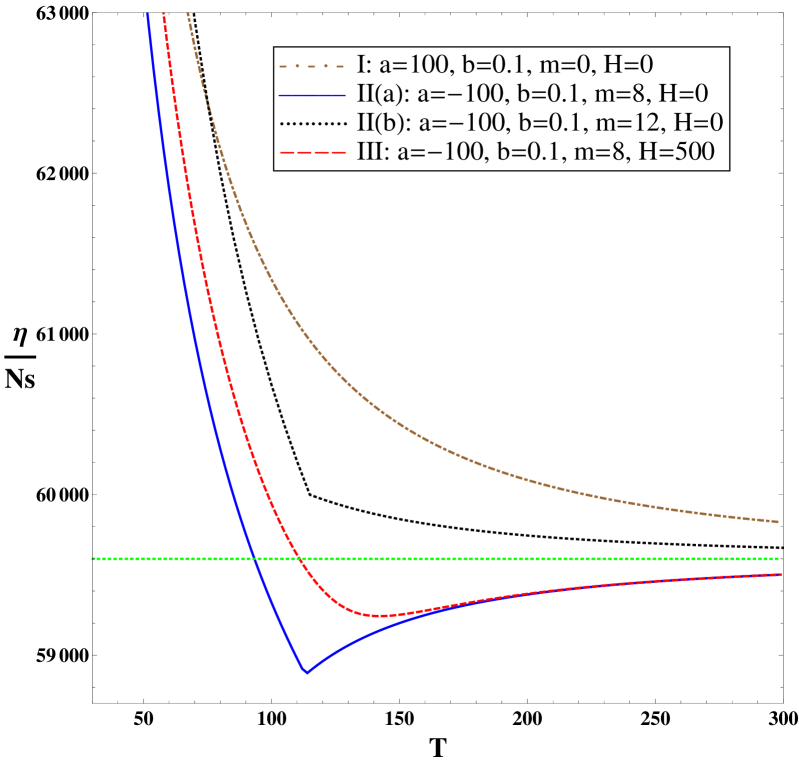
Figure 1: $\eta/(sN)$ vs. $T$ for cases with a second-order phase transition (solid and dotted curves), a crossover (dashed curve), and with no phase transition (dash-dotted curve). The horizontal dotted line is the asymptotic line for $\eta/(sN)$ at high $T$, which is calculated from the massless case. Parameter can be in arbitrary units.

In cases I-III, $\eta/s$ is monotonically decreasing near $T=0$. This is because $s$ approaches zero exponentially ($\pi$’s are massive) while $\eta$ approaches zero via power laws. This behavior persists even when $\pi$’s are massless, but by a different reason. In this case, below $T_{c}$,$\ \sigma$ can be integrated out. The resulting theory is a non-linear $\sigma$ model with massless goldstone bosons (the $\pi$’s) that couple derivatively to each other. So $\pi$’s become free particle at $T=0$, and the interaction becomes stronger at higher $T$. Tow show this more explicitly, when $m=H=0$, Eq.(12) can be recast as

$$\frac{|\mathcal{T}|^{2}}{4b^{2}}=\left|\frac{1}{1-m_{\sigma}^{2}/s}\right|^{2}+\left|\frac{1}{1-m_{\sigma}^{2}/t}\right|^{2}+\left|\frac{1}{1-m_{\sigma}^{2}/u}\right|^{2}.$$ (32)

Thus,

$$|\mathcal{T}|^{2}\propto\frac{T^{2}}{m_{\sigma}^{2}},$$ (33)

with $m_{\sigma}$ approaching a constant at small $T$, the couplings between pions are weaker at lower $T$ as mentioned above. And because smaller coupling implies larger $\eta/s$, $\eta/s$ decreases monotonically near $T=0$ for massless $\pi$’s.

As $T\rightarrow\infty$, all the systems are in the symmetric phase. The only scales in the problem are $m_{\pi}$ and $T$. We find that $\eta/s$ has the $1/T$ expansion

$$\frac{\eta}{s}=\frac{k_{0}N}{b^{2}}\left(1+\frac{k_{1}}{\sqrt{b}}\frac{a+m^{2}}{T^{2}}+\cdots\right)\ ,$$ (34)

with $k_{0}\simeq 571+80\sqrt{b}+\mathcal{O}(b)$ and $k_{1}\simeq 0.84-0.12\sqrt{b}+\mathcal{O}(b)$. The leading term in the expansion is the straight line in Fig. 1 which corresponds to the $\eta/s$ for a theory with $m=a=H=0$. (The slow running of the coupling $b$ has been neglected. $T$ is the only scale in the problem, so the dimensionless $\eta/s$ can only depend on the dimensionless coupling $b$ but not $T.$) The leading $T$ dependence comes from the $a+m^{2}$ term which has a positive sign for the symmetric phase ($a>0$). For the symmetric breaking phase ($a<0$), however, $a+m^{2}$ could still be positive. Numerically, this give a $\eta/s$ which does not reach a local minimum at $T_{c}$ for a second order phase transition as shown in case II(b) of Fig. 1.

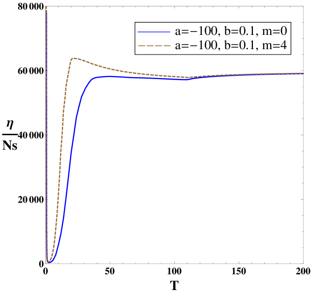
Figure 2: $\eta/(sN)$ vs. $T$ for cases where the resonance effects are important (the thermal width of $\sigma$ is included). A “double dip” behavior is seen with the $m=0$ case. Parameter can be in arbitrary units.

One might worry that whether case II(b) is qualified as a second order phase transition. After all, the order parameter is defined on one component $\phi_{N}$ whose mass is different from all the other $N-1$ components. If we remove the $\phi_{N}$, then the system does not have a phase transition in the first place. To answer this question, we study a similar model with just two real scalar fields new . One of the fields condenses below $T_{c}$ and the other stays in the symmetric phase. For simplicity, the interaction between the two fields is turned off. It is found that the $\eta/s$ behavior in this model is similar to that of II(b).

Our results of case II(a) and II(b) differ from that of Ref. Dobado:2009ek which has the minimum of $\eta/s$ below $T_{c}$. In Dobado:2009ek , the parameters of the Lagrangian are tuned to mimic the $\pi\pi$ scattering in the real world. Thus, the S-channel $\pi\pi$ scattering diagrams are resumed to reflect the strong $\pi\pi$ scattering in intermediate energies. In our case, we keep the coupling $b$ small and $2m_{\pi}>m_{\sigma}$ to make sure $\pi\pi$ scattering stays above the $\sigma$ resonance, such that we can apply the Boltzmann equation to compute $\eta$ reliably. If we set $m=0$, such that $m_{\pi}=0$ below $T_{c}$, then the $\sigma$ can become on-shell in $\pi\pi$ scattering when $T\simeq\mathcal{O}(m_{\sigma}|_{T=0})\simeq b^{1/2}T_{c}<T_{c}$. Then, indeed, a second local minimum (and sometimes also an absolute minimum, depending on the parameters) of $\eta/s$ below $T_{c}$ can be formed to have the “double dip” structure. Furthermore, it is conceivable that by tuning parameters, one can make the two local minimums to be close to each other and with the cusp at $T_{c}$ smoothed out such that one just sees the single minimum below $T_{c}$ as is shown in Dobado:2009ek . An $\eta/s$ plot with this feature is shown in Fig. 2 where the thermal width of $\sigma$ Nishikawa:2003  is included in the computation of $\eta$. However, the reader should be warned that while it might a generic feature to have a dip in $\eta/s$ below $T_{c}$ by a strong resonance, the $\eta$ computed with Boltzmann equation in this case might not be reliable as discussed in Section 2.

V Conclusion

We have discussed in details the computation procedure and the rich phenomena of the $\eta/s$ behavior in weakly coupled $N$-component real scalar field theories. We have found that $\eta/s$ can have a “double dip” behavior due to resonances and the phase transition. It is conceivable that by tuning parameters, one can make the two local minimums to be close to each other and with the cusp at $T_{c}$ smoothed out such that one just sees the single minimum below $T_{c}$ as is shown in Dobado:2009ek . If an explicit goldstone mass term is added, then $\eta/s$ can either decrease monotonically in temperature or, as seen in many other systems, reach a minimum at the phase transition. We have also shown how to go beyond the original variational approach to make the Boltzmann equation computation of $\eta$ systematic.

VI ACKNOWLEDGEMENTS

We thank Eiji Nakano and Di-Lun Yang for involvement in the early stage of this paper. We also thank Brian Smigielski for careful reading of the manuscript. JWC, CTH and HHL are supported by the NSC and NCTS of Taiwan. The work of M.H. is supported by NSFC10735040, NSFC10875134, and K.C.Wong Education Foundation, Hong Kong.

VII Appendix A: CJT Formalism

In this appendix we derive the effective potential of the Lagrangian

$$\mathcal{L}=\frac{1}{2}(\partial_{\mu}\vec{\phi})^{2}-\overrightarrow{H}\cdot\vec{\phi}-\frac{1}{2}a\vec{\phi}^{2}-\frac{1}{4}b\left(\vec{\phi}^{2}\right)^{2}-\frac{1}{6}c\left(\vec{\phi}^{2}\right)^{3}\ .$$ (35)

The $\overrightarrow{H}\cdot\vec{\phi}$ term is included so one can mimic a cross-over with a non-zero $\overrightarrow{H}$. The last term is a dimension six operator whose effect to $\eta/s$ is not studied in the main text but is included here for completeness. There could be two additional terms with dimension six: $\vec{\phi}^{2}\left(\vec{\phi}\cdot\partial^{2}\vec{\phi}\right)$, $\vec{\phi}\cdot\partial^{2}\partial^{2}\vec{\phi}$ (the other terms are related to these ones via integration by parts). These terms can be removed by field redefinition or, equivalently, by applying the equation of motion. The inclusion of the dimension six terms shows that this is an effective field theory, which is valid under the cut-off scale $1/\left(N\sqrt{c}\right)$ and is renormalized order by order in the momentum expansion $Np\sqrt{c}$, $p$ being a typical momentum scale in the problem. $a$, $b$, and $c$ are renormalized quantities and the counterterm Lagrangian is not shown. The renormalization condition is that the counterterms do not change the particle mass and the four- and six-point couplings at threshold.

We will use the standard Cornwall–Jackiw–Tomboulis (CJT) formalism CJT which has the one-particle irreducible diagrams included self-consistently. The effective potential in the CJT formalism reads:

$$V = \frac{a}{2}\overline{v}^{2}+\frac{b}{4}\overline{v}^{2}+\frac{c}{6}\overline{v}^{6}-H\overline{v}$$ (36)

$$+\frac{1}{2}\int_{K}\left[\ln S^{-1}+S_{0}^{-1}S-1\right]+\frac{N-1}{2}\int_{K}\left[\ln P^{-1}+P_{0}^{-1}P-1\right]$$

$$+\left(N+1\right)\left(N-1\right)\left(\frac{b}{4}+\frac{c}{2}\overline{v}^{4}\right)L_{P}^{2}$$

$$+3\left(\frac{b}{4}+\frac{5}{2}c\overline{v}^{2}\right)L_{S}^{2}+\left(N-1\right)\left(\frac{b}{2}+3c\overline{v}^{2}\right)L_{S}L_{P}$$

$$+\frac{c}{6}\left(N^{2}-1\right)\left(N+3\right)L_{P}^{3}+\frac{c}{2}\left(N^{2}-1\right)L_{P}^{2}L_{S}$$

$$+\frac{3c}{2}\left(N-1\right)L_{P}L_{S}^{2}+\frac{5c}{2}L_{S}^{3}\ ,$$

where $L_{S}=\int_{K}\,S(K,\overline{v})$ and $L_{P}=\int_{K}\,P(K,\overline{v})$, and where $S(S_{0})$ and $P(P_{0})$ are the full(tree-level) propagators:

$$S^{-1}(K,\overline{v}) = -K^{2}+m_{\sigma}^{2}(\overline{v})\;,\newline S_{0}^{-1}(K,\overline{v})=-K^{2}+m_{\sigma,0}^{2}(\overline{v})\;,$$

$$P^{-1}(K,\overline{v}) = -K^{2}+m_{\pi}^{2}(\overline{v})\;,\newline P_{0}^{-1}(K,\overline{v})=-K^{2}+m_{\pi,0}^{2}(\overline{v})\;,$$ (37)

with the tree-level masses $m_{\sigma,0}^{2}=a+3b\overline{v}^{2}+5c\overline{v}^{4}$ and $m_{\pi,0}^{2}=a+b\overline{v}^{2}+c\overline{v}^{4}$. The expression for $V$ is consistent with that of Lenaghan:1999si in the $c=0$ limit.

The self-consistent one- and two-point Green’s functions satisfy

$$\left.\frac{\delta V}{\delta\overline{v}}\right|_{\overline{v}=v,S=S(v),P=P(v)} \equiv 0\;,\;\;\;\left.\frac{\delta V}{\delta S}\right|_{\overline{v}=v,S=S(v),P=P(v)}\equiv 0\ ,$$

$$\left.\frac{\delta V}{\delta P}\right|_{\overline{v}=v,S=S(v),P=P(v)} \equiv 0\ .$$ (38)

These yield

$$H = v\left\{a+bv^{2}+cv^{4}+\left(3b+10cv^{2}\right)L_{S}\right.$$ (39)

$$+\left(N-1\right)\left(b+2cv^{2}\right)L_{P}+c\left(N^{2}-1\right)L_{P}^{2}$$

$$\left.+6c\left(N-1\right)L_{S}L_{P}+15cL_{S}^{2}\right\}\ .$$

$$m_{\sigma}^{2} = m_{\sigma,0}^{2}+\left(3b+30cv^{2}\right)L_{S}$$ (40)

$$+\left(N-1\right)\left(b+6cv^{2}\right)L_{P}+c\left(N^{2}-1\right)L_{P}^{2}$$

$$+6c\left(N-1\right)L_{S}L_{P}+15cL_{S}^{2}\ .$$

$$m_{\pi}^{2} = m_{\pi,0}^{2}+\left(b+6cv^{2}\right)L_{S}$$ (41)

$$+\left(N+1\right)\left(b+2cv^{2}\right)L_{P}+c\left(N-1\right)\left(N+3\right)L_{P}^{2}$$

$$+2c\left(N+1\right)L_{S}L_{P}+3cL_{S}^{2}\ .$$

In the large $N$, i.e. $N\rightarrow\infty$, limit, a sensible scaling is to make $m_{\sigma(\pi)}=\mathcal{O}(N^{0})$. This implies

$$b = \mathcal{O}(N^{-1})\ ,\ \ c=\mathcal{O}(N^{-2})\ ,$$

$$v = \mathcal{O}(N^{1/2})\ ,\ \ H=\mathcal{O}(N^{1/2})\ ,$$ (42)

and $V=\mathcal{O}(N)$. This is the scaling adopted in the main text. In this large $N$ limit, the non-tadpole type loop diagrams are subleading in the effective potential. Thus, the Hartree approximation, which neglects the non-tadpole type loop diagrams, gives the correct result in the large $N$ limit. For example, if $H=0$, the goldstone bosons remain massless below $T_{c}$ as required.

VIII Appendix B: $1/N$ Expansion of the Coupled Boltzmann Equations

In this appendix the leading contribution to the shear viscosity of an $\mathcal{O}(N)$ model in the large $N$ limit is derived. We start with the coupled Boltzmann equations:

$$\frac{p^{\mu}}{E_{p}^{\pi_{i}}}\partial_{\mu}f_{p}^{\pi_{i}}(x) = \frac{1}{2}\int_{123}d\Gamma_{12;3p}^{\pi_{i}\pi_{i}\rightarrow\pi_{i}\pi_{i}}\left\{f_{1}^{\pi_{i}}f_{2}^{\pi_{i}}F_{3}^{\pi_{i}}F_{p}^{\pi_{i}}-F_{1}^{\pi_{i}}F_{2}^{\pi_{i}}f_{3}^{\pi_{i}}f_{p}^{\pi_{i}}\right\}$$

$$+\sum_{j\neq i}\int_{123}d\Gamma_{12;3p}^{\pi_{i}\pi_{j}\rightarrow\pi_{i}\pi_{j}}\left\{f_{1}^{\pi_{j}}f_{2}^{\pi_{i}}F_{3}^{\pi_{j}}F_{p}^{\pi_{i}}-F_{1}^{\pi_{j}}F_{2}^{\pi_{i}}f_{3}^{\pi_{j}}f_{p}^{\pi_{i}}\right\}$$

$$+\sum_{j\neq i}\frac{1}{2}\int_{123}d\Gamma_{12;3p}^{\pi_{j}\pi_{j}\rightarrow\pi_{i}\pi_{i}}\left\{f_{1}^{\pi_{j}}f_{2}^{\pi_{j}}F_{3}^{\pi_{i}}F_{p}^{\pi_{i}}-F_{1}^{\pi_{j}}F_{2}^{\pi_{j}}f_{3}^{\pi_{i}}f_{p}^{\pi_{i}}\right\}$$

$$+\frac{1}{2}\int_{123}d\Gamma_{12;3p}^{\sigma\sigma\rightarrow\pi_{i}\pi_{i}}\left\{f_{1}^{\sigma}f_{2}^{\sigma}F_{3}^{\pi_{i}}F_{p}^{\pi_{i}}-F_{1}^{\sigma}F_{2}^{\sigma}f_{3}^{\pi_{i}}f_{p}^{\pi_{i}}\right\}$$

$$+\int_{123}d\Gamma_{12;3p}^{\pi_{i}\sigma\rightarrow\sigma\pi_{i}}\left\{f_{1}^{\pi_{i}}f_{2}^{\sigma}F_{3}^{\sigma}F_{p}^{\pi_{i}}-F_{1}^{\pi_{i}}F_{2}^{\sigma}f_{3}^{\sigma}f_{p}^{\pi_{i}}\right\}$$

$$+\int_{12}d\Gamma_{1;2p}^{\sigma\rightarrow\pi_{i}\pi_{i}}\left\{f_{1}^{\sigma}F_{2}^{\pi_{i}}F_{p}^{\pi_{i}}-F_{1}^{\sigma}F_{2}^{\sigma}f_{p}^{\pi_{i}}\right\}\ ,$$

$$\frac{p^{\mu}}{E_{p}^{\sigma}}\partial_{\mu}f_{p}^{\sigma}(x) = \frac{1}{2}\int_{123}d\Gamma_{12;3p}^{\sigma\sigma\rightarrow\sigma\sigma}\left\{f_{1}^{\sigma}f_{2}^{\sigma}F_{3}^{\sigma}F_{p}^{\sigma}-F_{1}^{\sigma}F_{2}^{\sigma}f_{3}^{\sigma}f_{p}^{\sigma}\right\}$$ (43)

$$+\sum_{i}\frac{1}{2}\int_{123}d\Gamma_{12;3p}^{\pi_{i}\pi_{i}\rightarrow\sigma\sigma}\left\{f_{1}^{\pi_{i}}f_{2}^{\pi_{i}}F_{3}^{\sigma}F_{p}^{\sigma}-F_{1}^{\pi_{i}}F_{2}^{\pi_{i}}f_{3}^{\sigma}f_{p}^{\sigma}\right\}$$

$$+\sum_{i}\int_{123}d\Gamma_{12;3p}^{\sigma\pi_{i}\rightarrow\pi_{i}\sigma}\left\{f_{1}^{\sigma}f_{2}^{\pi_{i}}F_{3}^{\pi_{i}}F_{p}^{\sigma}-F_{1}^{\sigma}F_{2}^{\pi_{i}}f_{3}^{\pi_{i}}f_{p}^{\sigma}\right\}$$

$$+\sum_{i}\frac{1}{2}\int_{12}d\Gamma_{12;p}^{\pi_{i}\pi_{i}\rightarrow\sigma}\left\{f_{1}^{\pi_{i}}f_{2}^{\pi_{i}}F_{p}^{\sigma}-F_{1}^{\pi_{i}}F_{2}^{\pi_{i}}f_{p}^{\sigma}\right\}\ .$$

The measure

$$d\Gamma_{12;3p}^{\pi_{i}\sigma\rightarrow\sigma\pi_{i}}\equiv|\mathcal{T}_{12;3p}^{\pi_{i}\sigma\rightarrow\sigma\pi_{i}}|^{2}\frac{(2\pi)^{4}\delta^{4}(k_{1}+k_{2}-k_{3}-p)}{2^{4}E_{1}^{\pi_{i}}E_{2}^{\sigma}E_{3}^{\sigma}E_{p}^{\pi_{i}}}\prod_{i=1}^{3}\frac{d^{3}\mathbf{k}_{i}}{(2\pi)^{3}}\ ,$$ (44)

and those for the other channels are defined analogously.

Note that the $\pi_{i}$ distribution is flavor independent. Thus, in Eq. (43), there are only two independent distributions $f^{\pi}\equiv f^{\pi_{i}}$ and $f^{\sigma}$. And the coupled Boltzmann equations can be written as:

$$\frac{p^{\mu}}{E_{p}^{\pi}}\partial_{\mu}f_{p}^{\pi}(x) = \frac{g_{\pi}}{2}\int_{123}d\Gamma_{12;3p}^{\pi\pi\rightarrow\pi\pi}\left\{f_{1}^{\pi}f_{2}^{\pi}F_{3}^{\pi}F_{p}^{\pi}-F_{1}^{\pi}F_{2}^{\pi}f_{3}^{\pi}f_{p}^{\pi}\right\}$$

$$+\frac{g_{\sigma}}{2}\int_{123}d\Gamma_{12;3p}^{\sigma\sigma\rightarrow\pi\pi}\left\{f_{1}^{\sigma}f_{2}^{\sigma}F^{\pi}F_{p}^{\pi}-F_{1}^{\sigma}F_{2}^{\sigma}f_{3}^{\pi}f_{p}^{\pi}\right\}$$

$$+g_{\sigma}\int_{123}d\Gamma_{12;3p}^{\pi\sigma\rightarrow\sigma\pi}\left\{f_{1}^{\pi}f_{2}^{\sigma}F_{3}^{\sigma}F_{p}^{\pi}-F_{1}^{\pi}F_{2}^{\sigma}f_{3}^{\sigma}f_{p}^{\pi}\right\}$$

$$+g_{\sigma}\int_{12}d\Gamma_{1;2p}^{\sigma\rightarrow\pi\pi}\left\{f_{1}^{\sigma}F_{2}^{\pi}F_{p}^{\pi}-F_{1}^{\sigma}f_{2}^{\pi}f_{p}^{\pi}\right\}\ ,$$

$$\frac{p^{\mu}}{E_{p}^{\sigma}}\partial_{\mu}f_{p}^{\sigma}(x) = \frac{g_{\sigma}}{2}\int_{123}d\Gamma_{12;3p}^{\sigma\sigma\rightarrow\sigma\sigma}\left\{f_{1}^{\sigma}f_{2}^{\sigma}F_{3}^{\sigma}F_{p}^{\sigma}-F_{1}^{\sigma}F_{2}^{\sigma}f_{3}^{\sigma}f_{p}^{\sigma}\right\}$$ (45)

$$+\frac{g_{\pi}}{2}\int_{123}d\Gamma_{12;3p}^{\pi\pi\rightarrow\sigma\sigma}\left\{f_{1}^{\pi}f_{2}^{\pi}F_{3}^{\sigma}F_{p}^{\sigma}-F_{1}^{\pi}F_{2}^{\pi}f_{3}^{\sigma}f_{p}^{\sigma}\right\}$$

$$+g_{\pi}\int_{123}d\Gamma_{12;3p}^{\sigma\pi\rightarrow\pi\sigma}\left\{f_{1}^{\sigma}f_{2}^{\pi}F_{3}^{\pi}F_{p}^{\sigma}-F_{1}^{\sigma}F_{2}^{\pi}f_{3}^{\pi}f_{p}^{\sigma}\right\}$$

$$+\frac{g_{\pi}}{2}\int_{12}d\Gamma_{12;p}^{\pi\pi\rightarrow\sigma}\left\{f_{1}^{\pi}f_{2}^{\pi}F_{p}^{\sigma}-F_{1}^{\pi}F_{2}^{\pi}f_{p}^{\sigma}\right\}\ ,$$

where $g_{\pi}=N-1$ and $g_{\sigma}=1$. The scattering amplitudes (squared) are related to those in Eq. (43) as

$$g_{\pi}\left|\mathcal{T}_{12;3p}^{\pi\pi\rightarrow\pi\pi}\right|^{2} = \left|\mathcal{T}_{12;3p}^{\pi_{i}\pi_{i}\rightarrow\pi_{i}\pi_{i}}\right|^{2}+2\left(g_{\pi}-1\right)\left|\mathcal{T}_{12;3p}^{\pi_{i}\pi_{j}\rightarrow\pi_{i}\pi_{j}}\right|^{2}+\left(g_{\pi}-1\right)\left|\mathcal{T}_{12;3p}^{\pi_{j}\pi_{j}\rightarrow\pi_{i}\pi_{i}}\right|^{2}$$ (46)

$$= \left|24\lambda_{1}+4g_{2}^{2}\left(\frac{1}{s-m_{\sigma}^{2}}+\frac{1}{t-m_{\sigma}^{2}}+\frac{1}{u-m_{\sigma}^{2}}\right)\right|^{2}$$

$$+2\left(g_{\pi}-1\right)\left|8\lambda_{3}+\frac{4g_{2}^{2}}{t-m_{\sigma}^{2}}\right|^{2}+\left(g_{\pi}-1\right)\left|8\lambda_{3}+\frac{4g_{2}^{2}}{s-m_{\sigma}^{2}}\right|^{2}\$$

$$\rightarrow N\left(2\left|8\lambda_{3}+\frac{4g_{2}^{2}}{t-m_{\sigma}^{2}}\right|^{2}+\left|8\lambda_{3}+\frac{4g_{2}^{2}}{s-m_{\sigma}^{2}}\right|^{2}\right)=\mathcal{O}(1/N).$$

$$\left|\mathcal{T}_{12;3p}^{\sigma\sigma\rightarrow\pi\pi}\right|^{2} = \left|\mathcal{T}_{12;3p}^{\pi\pi\rightarrow\sigma\sigma}\right|^{2}=\left|\mathcal{T}_{12;3p}^{\sigma\sigma\rightarrow\pi_{i}\pi_{i}}\right|^{2}\$$ (47)

$$= \left|4\lambda_{2}+\frac{12g_{1}g_{2}}{s-m_{\sigma}^{2}}+4g_{2}^{2}\left(\frac{1}{u-m_{\pi}^{2}}+\frac{1}{t-m_{\pi}^{2}}\right)\right|^{2}$$

$$= \mathcal{O}(1/N^{2})\ .$$

$$\left|\mathcal{T}_{12;3p}^{\sigma\sigma\rightarrow\sigma\sigma}\right|^{2} = \left|24\lambda_{1}+36g_{1}^{2}\left(\frac{1}{s-m_{\sigma}^{2}}+\frac{1}{t-m_{\sigma}^{2}}+\frac{1}{u-m_{\sigma}^{2}}\right)\right|^{2}$$ (48)

$$= \mathcal{O}(1/N^{2})\ .$$

$$\left|\mathcal{T}_{12;3p}^{\pi\sigma\rightarrow\sigma\pi}\right|^{2} = \left|\mathcal{T}_{12;3p}^{\sigma\pi\rightarrow\pi\sigma}\right|^{2}=\left|\mathcal{T}_{12;3p}^{\pi_{i}\sigma\rightarrow\sigma\pi_{i}}\right|^{2}$$ (49)

$$= \left|4\lambda_{2}+\frac{12g_{1}g_{2}}{u-m_{\sigma}^{2}}+4g_{2}^{2}\left(\frac{1}{s-m_{\pi}^{2}}+\frac{1}{t-m_{\pi}^{2}}\right)\right|^{2}$$

$$= \mathcal{O}(1/N^{2})\ .$$

$$\left|\mathcal{T}_{1;2p}^{\sigma\rightarrow\pi\pi}\right|^{2}\ =\left|2g_{2}\right|^{2}=\mathcal{O}(1/N)\ .$$ (50)

In the large $N$ limit, Eq.(45) is simplified to

$$\frac{p^{\mu}}{E_{p}^{\pi}}\partial_{\mu}f_{p}^{\pi}(x) = \frac{1}{2N}\int_{123}d\overline{\Gamma}_{12;3p}^{\pi\pi\rightarrow\pi\pi}\left\{f_{1}^{\pi}f_{2}^{\pi}F_{3}^{\pi}F_{p}^{\pi}-F_{1}^{\pi}F_{2}^{\pi}f_{3}^{\pi}f_{p}^{\pi}\right\}$$ (51)

$$+\frac{1}{N}\int_{12}d\overline{\Gamma}_{1;2p}^{\sigma\rightarrow\pi\pi}\left\{f_{1}^{\sigma}F_{2}^{\pi}F_{p}^{\pi}-F_{1}^{\sigma}f_{2}^{\pi}f_{p}^{\pi}\right\}\ ,$$

$$\frac{p^{\mu}}{E_{p}^{\sigma}}\partial_{\mu}f_{p}^{\sigma}(x) = +\frac{1}{2}\int_{12}d\overline{\Gamma}_{12;p}^{\pi\pi\rightarrow\sigma}\left\{f_{1}^{\pi}f_{2}^{\pi}F_{p}^{\sigma}-F_{1}^{\pi}F_{2}^{\pi}f_{p}^{\sigma}\right\},$$ (52)

where the $N$ dependence in $d\Gamma$ is factored out already, so all the $N$ dependence is in the prefactors. The above equations imply

$$\left(p_{i}p_{j}-\frac{1}{3}\delta_{ij}\mathbf{p}^{2}\right)$$

$$= \frac{E_{p}^{\pi}}{2N}\int_{123}d\overline{\Gamma}_{12;3p}^{\pi\pi\rightarrow\pi\pi}\overline{F}_{1}^{\pi}\overline{F}_{2}^{\pi}\overline{f}_{3}^{\pi}(\overline{F}_{p}^{\pi})^{-1}\left[B_{ij}^{\pi}(p)+B_{ij}^{\pi}(k_{3})-B_{ij}^{\pi}(k_{2})-B_{ij}^{\pi}(k_{1})\right]$$

$$+\frac{1}{N}E_{p}^{\pi}\int_{12}d\overline{\Gamma}_{1;2p}^{\sigma\rightarrow\pi\pi}\overline{F}_{1}^{\sigma}\overline{f}_{2}^{\pi}(\overline{F}_{p}^{\pi})^{-1}\left[B_{ij}^{\pi}(p)+B_{ij}^{\pi}(k_{2})-B_{ij}^{\sigma}(k_{1})\right],$$

$$\left(p_{i}p_{j}-\frac{1}{3}\delta_{ij}\mathbf{p}^{2}\right)$$

$$= \frac{E_{p}^{\sigma}}{2}\int_{12}d\overline{\Gamma}_{12;p}^{\pi\pi\rightarrow\sigma}\overline{F}_{1}^{\pi}\overline{F}_{2}^{\pi}(\overline{F}_{p}^{\sigma})^{-1}\left[B_{ij}^{\sigma}(p)-B_{ij}^{\pi}(k_{2})-B_{ij}^{\pi}(k_{1})\right],$$ (54)

where $B_{ij}$, defined in Eq.(15), describes how $\overline{f}$ changes when the velocity distribution is non-uniform. Eq.(VIII) demands $B_{ij}^{\pi}(p)=\mathcal{O}(N).$ Eq.(54) demands $B_{ij}^{\sigma}(p)=\mathcal{O}(N)$ such that Eq.(54) remains $\mathcal{O}(1)$. Now,

$$\eta = NL^{\pi}\left[B^{\pi}\right]+L^{\sigma}\left[B^{\sigma}\right]\ ,$$

$$L^{l}\left[B^{l}\right] = \frac{\beta}{15}\int\frac{\mathrm{d}^{3}\mathbf{p}\,\mathbf{p}^{2}}{(2\pi)^{3}E_{p}^{k}}\overline{f}_{p}^{l}\overline{F}_{p}^{l}B^{l}(p)\$$ (55)

In the large $N$ limit

$$\eta = NL^{\pi}\left[B^{\pi}\right]\$$ (56)

$$\simeq NL^{\pi}\left[B^{\pi}\right]+cL^{\sigma}\left[B^{\sigma}\right],$$

where we have added a subleading term with prefactor $c\sim\mathcal{O}(N^{0})$. The final result for $\eta$ should not depend on the choice of $c$.

Substituting Eqs.(VIII,54) into Eq.(56), one obtains

$$\eta = \frac{\beta}{20}\int_{123p}d\overline{\Gamma}_{12;3p}^{\pi\pi\rightarrow\pi\pi}\overline{F}_{1}^{\pi}\overline{F}_{2}^{\pi}\overline{f}_{3}^{\pi}\overline{f}_{p}^{\pi}B_{ij}^{\pi}(p)\left[B_{ij}^{\pi}(p)+B_{ij}^{\pi}(k_{3})-B_{ij}^{\pi}(k_{2})-B_{ij}^{\pi}(k_{1})\right]$$ (57)

$$+\frac{\beta}{10}\int_{12p}d\overline{\Gamma}_{1;2p}^{\sigma\rightarrow\pi\pi}\overline{F}_{1}^{\sigma}\overline{f}_{2}^{\pi}\overline{f}_{p}^{\pi}B_{ij}^{\pi}(p)\left[B_{ij}^{\pi}(p)+B_{ij}^{\pi}(k_{2})-B_{ij}^{\sigma}(k_{1})\right]$$

$$+\frac{\beta c}{20}\int_{12p}d\overline{\Gamma}_{12;p}^{\pi\pi\rightarrow\sigma}\overline{F}_{1}^{\pi}\overline{F}_{2}^{\pi}\overline{f}_{p}^{\sigma}B_{ij}^{\sigma}(p)\left[B_{ij}^{\sigma}(p)-B_{ij}^{\pi}(k_{2})-B_{ij}^{\pi}(k_{1})\right].$$

Symmetries of the equations further gives

$$\eta = \frac{\beta}{80}\int_{123p}d\overline{\Gamma}_{12;3p}^{\pi\pi\rightarrow\pi\pi}\overline{F}_{1}^{\pi}\overline{F}_{2}^{\pi}\overline{f}_{3}^{\pi}\overline{f}_{p}^{\pi}\left[B_{ij}^{\pi}(p)+B_{ij}^{\pi}(k_{3})-B_{ij}^{\pi}(k_{2})-B_{ij}^{\pi}(k_{1})\right]^{2}$$ (58)

$$+\frac{\left(2+c\right)\beta}{60}\int_{12p}d\overline{\Gamma}_{1;2p}^{\sigma\rightarrow\pi\pi}\overline{F}_{1}^{\sigma}\overline{f}_{2}^{\pi}\overline{f}_{p}^{\pi}\left[B_{ij}^{\pi}(p)+B_{ij}^{\pi}(k_{2})-B_{ij}^{\sigma}(k_{1})\right]^{2}.$$

By choosing $c=-2$, the subleading contribution can be subtracted. Thus, $\overline{f}^{\sigma}$and $B_{ij}^{\sigma}$ decouple from $\eta$ and the $\sigma$ contribution only appears in the intermediate states of $\pi\pi$ scattering.

In summery, in the large $N$ limit, one can use

$$\eta = \frac{N\beta}{10}\int\frac{\mathrm{d}^{3}\mathbf{p}}{(2\pi)^{3}E_{p}}\overline{f}_{p}^{\pi}\overline{F}_{p}^{\pi}\left(p_{i}p_{j}-\frac{1}{3}\delta_{ij}\mathbf{p}^{2}\right)B_{ij}(p)$$ (59)

$$= \frac{\beta}{80}\int_{123p}d\overline{\Gamma}_{12;3p}^{\pi\pi\rightarrow\pi\pi}\overline{F}_{1}^{\pi}\overline{F}_{2}^{\pi}\overline{f}_{3}^{\pi}\overline{f}_{p}^{\pi}\left[B_{ij}^{\pi}(p)+B_{ij}^{\pi}(k_{3})-B_{ij}^{\pi}(k_{2})-B_{ij}^{\pi}(k_{1})\right]^{2}\text{,}$$

to solve $B_{ij}^{\pi}$ and $\eta$.

References

- (1) S. Jeon, Phys. Rev. D 52, 3591 (1995); S. Jeon and L. Yaffe, Phys. Rev. D 53, 5799 (1996).
- (2) P. Kovtun, D.T. Son, and A.O. Starinets, Phys. Rev. Lett. 94,111601 (2005).
- (3) G. Policastro, D.T. Son, and A.O. Starinets, Phys. Rev. Lett. 87, 081601 (2001).
- (4) G. Policastro, D. T. Son and A. O. Starinets, JHEP 0209, 043 (2002).
- (5) C.P. Herzog, J. High Energy Phys. 0212, 026 (2002).
- (6) A. Buchel and J.T. Liu, Phys. Rev. Lett. 93, 090602 (2004).
- (7) D. T. Son and A. O. Starinets, Ann. Rev. Nucl. Part. Sci. 57, 95 (2007) [arXiv:0704.0240 [hep-th]].
- (8) J. I. Kapusta, arXiv:0809.3746 [nucl-th].
- (9) T. Schafer and D. Teaney, Rept. Prog. Phys. 72, 126001 (2009) [arXiv:0904.3107 [hep-ph]].
- (10) A. Jakovac, Phys. Rev. D81: 045020 (2010).
- (11) T. D. Cohen, Phys. Rev. Lett. 99, 021602 (2007) [arXiv:hep-th/0702136].
- (12) A. Cherman, T. D. Cohen and P. M. Hohler, JHEP 0802, 026 (2008) [arXiv:0708.4201 [hep-th]].
- (13) Y. Kats and P. Petrov, JHEP 0901, 044 (2009) [arXiv:0712.0743 [hep-th]].
- (14) M. Brigante, H. Liu, R. C. Myers, S. Shenker and S. Yaida, Phys. Rev. D 77, 126006 (2008) [arXiv:0712.0805 [hep-th]].
- (15) M. Brigante, H. Liu, R. C. Myers, S. Shenker and S. Yaida, Phys. Rev. Lett. 100, 191601 (2008) [arXiv:0802.3318 [hep-th]].
- (16) A. Buchel, R. C. Myers and A. Sinha, JHEP 0903, 084 (2009) [arXiv:0812.2521 [hep-th]].
- (17) M. Gyulassy and L. McLerran, Nucl. Phys. A 750, 30 (2005) [arXiv:nucl-th/0405013].
- (18) E. V. Shuryak, Nucl. Phys. A 750, 64 (2005) [arXiv:hep-ph/0405066].
- (19) H. Stoecker, Nucl. Phys. A 750, 121 (2005) [arXiv:nucl-th/0406018].
- (20) P. Jacobs and X. N. Wang, Prog. Part. Nucl. Phys. 54, 443 (2005) [arXiv:hep-ph/0405125].
- (21) I. Arsene et al., Nucl. Phys. A 757, 1 (2005); B. B. Back et al., ibid. 757, 28 (2005); J. Adams et al., ibid. 757, 102 (2005); K. Adcox et al., ibid. 757, 184 (2005).
- (22) P. Huovinen, P. F. Kolb, U. W. Heinz, P. V. Ruuskanen and S. A. Voloshin, Phys. Lett. B 503, 58 (2001) [arXiv:hep-ph/0101136].
- (23) D. Teaney, J. Lauret and E. V. Shuryak, Phys. Rev. Lett. 86, 4783 (2001) [arXiv:nucl-th/0011058].
- (24) A. Muronga and D. H. Rischke, arXiv:nucl-th/0407114.
- (25) U. W. Heinz, H. Song and A. K. Chaudhuri, Phys. Rev. C 73, 034904 (2006) [arXiv:nucl-th/0510014].
- (26) P. Romatschke and U. Romatschke, Phys. Rev. Lett. 99, 172301 (2007) [arXiv:0706.1522 [nucl-th]].
- (27) T. Hirano and K. Tsuda, Phys. Rev. C 66, 054905 (2002) [arXiv:nucl-th/0205043].
- (28) D. Molnar and M. Gyulassy, Nucl. Phys. A 697, 495 (2002) [Erratum ibid. 703, 893 (2002)].
- (29) D. Teaney, Phys. Rev. C 68, 034913 (2003).
- (30) M. Luzum and P. Romatschke, Phys. Rev. C 78, 034915 (2008) [arXiv:0804.4015 [nucl-th]].
- (31) H. Song and U. W. Heinz, J. Phys. G 36, 064033 (2009) [arXiv:0812.4274 [nucl-th]].
- (32) H. B. Meyer, Phys. Rev. D 76, 101701 (2007), arXiv:0704.1801 [hep-lat].
- (33) T. Schafer, Phys. Rev. A 76, 063618 (2007).
- (34) A. Turlapov, J. Kinast, B. Clancy, L. Luo, J. Joseph, and J. E. Thomas, J. Low Temp. Phys. 150, 567 (2008).
- (35) B. Clancy, L. Luo, J. E. Thomas Phys. Rev. Lett. 99 140401 (2007) [arXiv:0705.2782 [condmat.other]].
- (36) J.E. Thomas, Nucl. Phys. A 830, 665c (2009).
- (37) T. Schaefer, C. Chafin, e-Print: arXiv:0912.4236 [cond-mat.quant-gas]; T. Schaefer, e-Print: arXiv:1008.3876 [cond-mat.quant-gas].
- (38) L. P. Csernai, J. I. Kapusta and L. D. McLerran, Phys. Rev. Lett. 97, 152303 (2006).
- (39) J. W. Chen and E. Nakano, Phys. Lett. B 647, 371 (2007).
- (40) J. W. Chen, M. Huang, Y. H. Li, E. Nakano and D. L. Yang, Phys. Lett. B 670, 18 (2008) [arXiv:0709.3434 [hep-ph]].
- (41) G. Aarts and J. M. Martinez Resco, Phys. Rev. D 68, 085009 (2003); JHEP 0402, 061 (2004).
- (42) G. D. Moore, Phys. Rev. D76: 107702, 2007.
- (43) A. Dobado, F. J. Llanes-Estrada and J. M. Torres-Rincon, Phys. Rev. D 80, 114015 (2009) [arXiv:0907.5483 [hep-ph]].
- (44) P. Chakraborty, J.I. Kapusta, arXiv:1006.0257 [nucl-th]
- (45) P. Arnold, G. D. Moore and L. G. Yaffe, JHEP 0305, 051 (2003) [arXiv:hep-ph/0302165]; P. Arnold, Int. J. Mod. Phys. E 16, 2555 (2007) [arXiv:0708.0812 [hep-ph]].
- (46) Z. Xu and C. Greiner, Phys. Rev. Lett. 100, 172301 (2008) [arXiv:0710.5719 [nucl-th]].
- (47) J. W. Chen, H. Dong, K. Ohnishi and Q. Wang, Phys. Lett. B 685, 277 (2010) [arXiv:0907.2486 [nucl-th]].
- (48) M. Prakash, M. Prakash, R. Venugopalan and G. Welke, Phys. Rept. 227, 321 (1993).
- (49) A. Dobado and F. J. Llanes-Estrada, Phys. Rev. D 69 (2004) 116004 [arXiv:hep-ph/0309324].
- (50) A. Dobado and S. N. Santalla, Phys. Rev. D 65, 096011 (2002) [arXiv:hep-ph/0112299].
- (51) K. Itakura, O. Morimatsu and H. Otomo, Phys. Rev. D 77, 014014 (2008) [arXiv:0711.1034 [hep-ph]].
- (52) J. W. Chen, Y. H. Li, Y. F. Liu and E. Nakano, Phys. Rev. D76, 114011(2007).
- (53) T. Schafer, arXiv:cond-mat/0701251; G. Rupak and T. Schafer, arXiv:0707.1520 [cond-mat.other].
- (54) E.W. Lemmon et al., Thermophysical Properties of Fluid Systems, in NIST Chemistry WebBook, NIST Standard Reference Database Number 69, Eds. Linstrom P.G. & Mallard, W.G., March 2003 (http://webbook.nist.gov).
- (55) R. A. Lacey et al., Phys. Rev. Lett. 98, 092301 (2007); arXiv:0708.3512.
- (56) J. S. Gagnon and S. Jeon, Phys. Rev. D 76, 105019 (2007) [arXiv:0708.1631 [hep-ph]].
- (57) J.M. Cornwall, R. Jackiw, and E. Tomboulis, Phys. Rev. D 10, 2428 (1974).
- (58) P. Résibois and M. d. Leener, Classical Kinetic Theory of Fluids (John Wiley Sons, 1977).
- (59) J.W. Chen, C.T. Hsieh, H.H. Lin, in preparation.
- (60) T. Nishikawa, O. Morimatsu, and Y. Hidaka, Phys. Rev. D 68, 076002 (2003) [arXiv:hep-ph/0302098].
- (61) J. T. Lenaghan and D. H. Rischke, J. Phys. G 26, 431 (2000) [arXiv:nucl-th/9901049].