Investigation of heavy-heavy pseudoscalar mesons in thermal QCD Sum Rules

Abstract

We investigate the mass and decay constant of the heavy-heavy pseudoscalar, $B_{c}$, $\eta_{c}$ and $\eta_{b}$ mesons in the framework of finite temperature QCD sum rules. The annihilation and scattering parts of spectral density are calculated in the lowest order of perturbation theory. Taking into account the additional operators arising at finite temperature, the nonperturbative corrections are also evaluated. The masses and decay constants remain unchanged under $T\cong 100~{}MeV$, but after this point, they start to diminish with increasing the temperature. At critical or deconfinement temperature, the decay constants reach approximately to 38% of their values in the vacuum, while the masses are decreased about 5%, 10% and 2% for $B_{c}$, $\eta_{c}$ and $\eta_{b}$ states, respectively. The results at zero temperature are in a good consistency with the existing experimental values as well as predictions of the other nonperturbative approaches.

I Introduction

Over the last two decades, there is an increasing interest on properties of hadrons under extreme conditions K.Yagi ; J.Letessier . According to these investigations, two theoretical aspects, namely theoretical studies of hadrons at finite temperature and density as well as a careful analysis of the heavy ion collision results are important. Calculation of hadronic parameters at finite temperature and density directly from QCD is a difficult problem. The thermal QCD is successful theory in the large momentum transfer region, where the quark-gluon running coupling constant is small and one can reliably use perturbative approaches. However, at the hadronic scale, this coupling constant becomes large and perturbation theories fail. Hence, investigation of hadronic properties requires some nonperturbative approaches. Some nonperturbative approaches are lattice QCD, heavy quark effective theory (HQET), different quark models and QCD sum rules. Among these approaches, the QCD sum rule method M.A.Shifman and its extension to the finite temperature A.I.Bochkarev has been extensively used as an efficient tool to hadron physics P.Colangelo . The same as QCD sum rules in vacuum, the main idea in thermal QCD sum rules also is to relate the hadronic parameters with the QCD degrees of freedom. In this method, an appreciate thermal correlator is expressed in terms of interpolating currents of participating particles. From one side, this correlation function is evaluated saturating it by a tower of hadrons with the same quantum numbers as the interpolating currents. On the other hand, it is calculated via the operator product expansion (OPE) in terms of operators having different mass dimensions. Matching these two different representations of the same correlation function provides us a possibility to predict hadronic properties in terms of finite-temperature perturbation theory and long-distance nonperturbative physics including the thermal quark and gluon condensates as well as thermal average of energy density.

Comparing to the QCD sum rules in vacuum, the thermal QCD sum rules have several new features. One of them is to take into account the interaction of the currents with the existing particles in the medium. Such interactions require modification of the hadronic spectral function. The other aspect is breakdown of Lorentz invariance by the choice of reference frame. Due to residual $O(3)$ symmetry at finite temperature, more operators with the same dimensions appear in the OPE compared to those at zero temperature E.V.Shuryak ; T.Hatsuda ; S.Mallik . The thermal QCD sum rule method has been extensively used to study the thermal properties of light S.Mallik1 ; S.Mallik2 ; E.V.Veliev , heavy-light C.A.Dominguez1 ; C.A.Dominguez2 ; E.V.Veliev1 and heavy-heavy F.Klingl ; K.Morita ; K.Morita1 ; E.V.Veliev2 mesons as a reliable and well-established method.

The discussion of heavy mesons properties at zero temperature has a rather long history V.A.Novikov ; T.M.Aliev ; L.J.Reinders ; I.I.Balitsky ; C.A.Dominguez ; T.M.Aliev1 ; S.S.Gershtein ; P.Ball ; S.Narison ; V.V.Kiselev ; M.Jamin ; TWChiu ; W.Wang ; T.M.Aliev2 ; T.M.Aliev3 . The heavy mesons play very important role in our understanding of nonperturbative dynamics of QCD. First determinations of leptonic decay constant of pseudoscalar, $B_{c}$ meson at zero temperature were made twenty years ago T.M.Aliev1 ; S.S.Gershtein . Such charged meson decays play important role to extract the magnitudes and phases of the Cabbibo-Kobayashi-Maskawa(CKM) matrix elements, which can help us understand the origins of CP violation in and beyond the standard model. Our aim in this work is to investigate the temperature dependence of mass and leptonic decay constants of the pseudoscalar $B_{c}$, $\eta_{c}$ and $\eta_{b}$ mesons taking into account the additional operators arising at finite temperature. The pseudoscalar decay constant, $f_{P}$ is defined by vacuum to meson matrix element of the axial vector current as:

$${\langle}0|(\overline{Q}_{1}\gamma_{\mu}\gamma_{5}Q_{2})(0)|P{\rangle}=if_{P}q_{\mu},$$ (1)

where $Q_{1,2}=c$ or $b$ and $P=B_{c},\eta_{c}$ or $\eta_{b}$. In thermal field theories, the meson mass, $m_{P}$ and its decay constant, $f_{P}$ should be replaced by their temperature dependent versions.

The paper is organized as follows. In section 2, we obtain thermal QCD sum rules for the masses and decay constants of the considered pseudoscalar mesons calculating the spectral densities and nonperturbative corrections. In section 3, we present our numerical calculations and discussions.

II Thermal QCD Sum Rules for Decay Constants and Masses of Heavy Pseudoscalar, $B_{c},\eta_{c}$ and $\eta_{b}$ Mesons

Taking into account the new aspects of the finite temperature QCD, sum rules for the masses and decay constants of the heavy pseudoscalar mesons containing $b$ and/or $c$ quark are derived in this section. The starting point is to consider the following responsible two-point thermal correlation function:

$$\Pi(q,T)=i\int d^{4}xe^{iq\cdot x}{\langle}{\cal T}\left(J^{P}(x)J^{P{\dagger}}(0)\right){\rangle},$$ (2)

where $T$ denotes the temperature, ${\cal T}$ is the time ordering product and $J^{P}(x)=\overline{Q}_{1}(x)i\gamma_{5}Q_{2}(x)$ is the interpolating current of the heavy pseudoscalar mesons. The thermal average of the operator, $A={\cal T}\left(J^{P}(x)J^{P{\dagger}}(0)\right)$ appearing in the above correlation function is expressed as:

$${\langle}A{\rangle}=\frac{Tr(e^{-\beta H}A)}{Tr(e^{-\beta H})},$$ (3)

where $H$ is the QCD Hamiltonian, $\beta=1/T$ is inverse of the temperature $T$ and traces are performed over any complete set of states.

As we previously mentioned, to obtain sum rules for physical observables, we need to calculate the aforementioned correlation function in two different ways. In QCD or theoretical side, the correlation function is calculated in deep Euclidean region, $q^{2}\ll-\Lambda_{QCD}^{2}$ via OPE where the short or perturbative and long distance or nonperturbative contributions are separated,

$$\Pi^{QCD}(q,T)=\Pi^{pert}(q,T)+\Pi^{nonpert}(q,T).$$ (4)

The perturbative contribution is calculated using perturbation theory, whereas the nonperturbative contributions are expressed in terms of the thermal expectation values of the quark and gluon condensates as well as thermal average of the energy density. The perturbative part can be written in terms of a dispersion integral, hence

$$\Pi^{QCD}(q,T)=\int\frac{ds\rho(s,T)}{s-q^{2}}+\Pi^{nonpert}(q,T),$$ (5)

where, $\rho(s,T)$ is called the spectral density at finite temperature. The thermal spectral density at fixed $|\bf{q}|$ is written as:

$$\rho(q,T)=\frac{1}{\pi}~{}Im\Pi^{pert}(q,T)~{}\tanh\left(\frac{\beta q_{0}}{2}\right).$$ (6)

In order to calculate the $\rho(q,T)$ in the lowest order in perturbation theory, we use quark propagator at finite temperature A.Das as:

$$S(q)=(\gamma_{\mu}~{}q^{\mu}+m)\left(\frac{1}{q^{2}-m^{2}+i\varepsilon}+2\pi in(|q_{0}|)~{}\delta(q^{2}-m^{2})\right),$$ (7)

where $n(x)=\left[exp(\beta x)+1\right]^{-1}$ is the Fermi distribution function. Using the above propagator, after some calculations we find the imaginary part of the correlation function as:

$$Im\Pi(q,T)=L(q_{0})+L(-q_{0}),$$ (8)

where,

$$L(q_{0}) = -N_{c}\int\frac{d\textbf{k}}{8\pi^{2}}\frac{\omega_{1}^{2}-\textbf{k}^{2}+\textbf{k}\cdot\textbf{q}-\omega_{1}q_{0}-m_{1}m_{2}}{\omega_{1}\omega_{2}}\Big{\{}\Big{[}\Big{(}1-n_{1}(\omega_{1})\Big{)}\Big{(}1-n_{2}(\omega_{2})\Big{)}+n_{1}(\omega_{1})n_{2}(\omega_{2})\Big{]}\delta(q_{0}-\omega_{1}-\omega_{2})$$ (9)

$$- \Big{[}\Big{(}1-n_{1}(\omega_{1})\Big{)}n_{2}(\omega_{2})+\Big{(}1-n_{2}(\omega_{2})\Big{)}n_{1}(\omega_{1})\Big{]}\delta(q_{0}-\omega_{1}+\omega_{2})\Big{\}}.$$

Here, $\omega_{1}=\sqrt{\textbf{k}^{2}+m_{1}^{2}}$ and $\omega_{2}=\sqrt{\textbf{(q-k)}^{2}+m_{2}^{2}}$. As it is seen, the $L(q_{0})$ involves two pieces. The first term, which includes delta function $\delta(q_{0}-\omega_{1}-\omega_{2})$ survives at zero temperature and is called the annihilation term. The second term, which includes delta function $\delta(q_{0}-\omega_{1}+\omega_{2})$ is called scattering term and vanishes at $T=0$. The delta function, $\delta(q_{0}-\omega_{1}-\omega_{2})$ in Eq. (9) gives the first branch cut, $q^{2}\geq(m_{1}+m_{2})^{2}$, which coincides with zero temperature cut that describes the standard threshold for particle decays. On the other hand, the delta function, $\delta(q_{0}-\omega_{1}+\omega_{2})$ in Eq. (9) shows that an additional branch cut arise at finite temperature, $q^{2}\leq(m_{1}-m_{2})^{2}$, which corresponds to particle absorption from the medium. Taking into account these contributions, the annihilation and scattering parts of spectral density in the case, $\textbf{q}=0$ can be written as:

$$\rho^{a,pert}(s,T)=\rho_{0}(s)\Big{[}1-n\Big{(}\frac{\sqrt{s}}{2}\Big{(}1+\frac{m_{1}^{2}-m_{2}^{2}}{s}\Big{)}\Big{)}-n\Big{(}\frac{\sqrt{s}}{2}\Big{(}1-\frac{m_{1}^{2}-m_{2}^{2}}{s}\Big{)}\Big{)}\Big{]},$$ (10)

for $(m_{1}+m_{2})^{2}\leq s\leq\infty$, and

$$\rho^{s,pert}(s,T)=\rho_{0}(s)\Big{[}n\Big{(}\frac{\sqrt{s}}{2}\Big{(}1+\frac{m_{1}^{2}-m_{2}^{2}}{s}\Big{)}\Big{)}-n\Big{(}-\frac{\sqrt{s}}{2}\Big{(}1-\frac{m_{1}^{2}-m_{2}^{2}}{s}\Big{)}\Big{)}\Big{]},$$ (11)

for $0\leq s\leq(m_{1}-m_{2})^{2}$ with $m_{1}\geq m_{2}$. Here $\rho_{0}(s)$, is the spectral density in the lowest order of perturbation theory at zero temperature and is given by:

$$\rho_{0}(s)=\frac{3}{8\pi^{2}s}q^{2}(s)v(s),$$ (12)

where $q(s)=s-(m_{1}-m_{2})^{2}$ and $v(s)=\sqrt{1-4m_{1}m_{2}/q(s)}$.

In our calculations, we also take into account the perturbative two-loop order $\alpha_{s}$ correction to the spectral density. For equal quark masses case this correction at zero temperature can be written as L.J.Reinders :

$$\rho_{\alpha_{s}}(s)=\frac{s\alpha_{s}v}{2\pi^{3}}\Big{[}\frac{\pi^{2}}{2v}-\frac{1+v}{2}\Big{(}\frac{\pi^{2}}{2}-3\Big{)}+F(v)\ln\frac{1+v}{1-v}+G(v)\Big{]},$$ (13)

where $F(v)$ and $G(v)$ functions have the following forms:

$$F(v)=\frac{3}{4v^{3}}-\frac{21}{16v}-\frac{18v}{16}+\frac{3v^{3}}{16},$$ (14)

and

$$G(v)=-\frac{3}{2v^{2}}+\frac{9}{8}-\frac{3v^{2}}{8}.$$ (15)

Here $v=v(s)$ and we replace the strong coupling $\alpha_{s}$ in Eq. (13) with its temperature dependent lattice improved expression K.Morita ; O.Kaczmarek . When doing the numerical calculations for $B_{c}$ meson, the contribution coming from two-loop diagrams is used for unequal quark masses case $\rho_{\alpha_{s}}$ L.J.Reinders ; C.A.Dominguez , but since its expression is very lengthy, we do not present its explicit expression here.

To calculate the nonperturbative part in QCD side, we use the nonperturbative part of the quark propagator in an external gluon field, $A^{a}_{\mu}(x)$ in the Fock-Schwinger gauge, $x^{\mu}A^{a}_{\mu}(x)=0$. Taking into account one and two gluon lines attached to the quark line, the massive quark propagator in momentum space can be written as L.J.Reinders :

$$S^{aa^{\prime}}(k) = \frac{i}{\not\!k-m}\delta^{aa^{\prime}}-\frac{i}{4}g(t^{c})^{aa^{\prime}}G^{c}_{\kappa\lambda}(0)\frac{1}{(k^{2}-m^{2})^{2}}\Big{[}\sigma_{\kappa\lambda}(\not\!k+m)+(\not\!k+m)\sigma_{\kappa\lambda}\Big{]}$$ (16)

$$- \frac{i}{4}g^{2}(t^{c}t^{d})^{aa^{\prime}}G^{c}_{\alpha\beta}(0)G^{d}_{\mu\nu}(0)\frac{\not\!k+m}{(k^{2}-m^{2})^{5}}(f_{\alpha\beta\mu\nu}+f_{\alpha\mu\beta\nu}+f_{\alpha\mu\nu\beta})(\not\!k+m),$$

where,

$$f_{\alpha\beta\mu\nu}=\gamma_{\alpha}(\not\!k+m)\gamma_{\beta}(\not\!k+m)\gamma_{\mu}(\not\!k+m)\gamma_{\nu}.$$ (17)

In order to proceed, we also need to know the expectation value, $\langle TrG_{\alpha\beta}G_{\mu\nu}\rangle$. The Lorentz covariance at finite temperature allows us to write the general structure of this expectation value in the following way:

$$\langle Tr^{c}G_{\alpha\beta}G_{\mu\nu}\rangle = \frac{1}{24}(g_{\alpha\mu}g_{\beta\nu}-g_{\alpha\nu}g_{\beta\mu})\langle G^{a}_{\lambda\sigma}G^{a\lambda\sigma}\rangle$$ (18)

$$+ \frac{1}{6}\Big{[}g_{\alpha\mu}g_{\beta\nu}-g_{\alpha\nu}g_{\beta\mu}-2(u_{\alpha}u_{\mu}g_{\beta\nu}-u_{\alpha}u_{\nu}g_{\beta\mu}-u_{\beta}u_{\mu}g_{\alpha\nu}+u_{\beta}u_{\nu}g_{\alpha\mu})\Big{]}\langle u^{\lambda}{\Theta}^{g}_{\lambda\sigma}u^{\sigma}\rangle,$$

where, $u^{\mu}$ is the four-velocity of the heat bath and it is introduced to restore Lorentz invariance formally in the thermal field theory. In the rest frame of the heat bath, $u^{\mu}=(1,0,0,0)$ and $u^{2}=1$. Also $\Theta^{g}_{\lambda\sigma}$ is the traceless, gluonic part of the stress-tensor of the QCD. Therefore, up to terms necessary for our calculations, the non perturbative part of massive quark propagator at finite temperature takes the form:

$$S^{aa^{\prime}nonpert}(k) = -\frac{i}{4}g(t^{c})^{aa^{\prime}}\frac{G^{c}_{\kappa\lambda}}{(k^{2}-m^{2})^{2}}\Big{[}\sigma_{\kappa\lambda}(\not\!k+m)+(\not\!k+m)\sigma_{\kappa\lambda}\Big{]}+\frac{i~{}g^{2}~{}\delta^{aa^{\prime}}}{9~{}(k^{2}-m^{2})^{4}}\Big{\{}\frac{3m(k^{2}+m\not\!k)}{4}\langle G^{c}_{\alpha\beta}G^{c\alpha\beta}\rangle$$ (19)

$$+ \Big{[}m\Big{(}k^{2}-4(k\cdot u)^{2}\Big{)}+\Big{(}m^{2}-4(k\cdot u)^{2}\Big{)}\not\!k+4(k\cdot u)(k^{2}-m^{2})\not\!u\Big{]}\langle u^{\alpha}\Theta^{g}_{\alpha\beta}u^{\beta}\rangle\Big{\}},$$

Using the above expression and after straightforward calculations, the nonperturbative part in QCD side is obtained as:

$$\Pi^{nonpert} = \int_{0}^{1}~{}dx\Big{\{}\frac{\langle\alpha_{s}G^{2}\rangle}{48\pi\Big{[}m_{1}^{2}(-1+x)-\Big{(}m_{2}^{2}+q^{2}(-1+x)\Big{)}x\Big{]}^{4}}\Big{[}-m_{1}^{6}(-1+x)^{4}(5-20x+3x^{2})+m_{1}^{5}m_{2}(-1+x)^{2}$$ (20)

$$\times (5-6x+12x^{2}-14x^{3}+6x^{4})-x^{4}\Big{(}24~{}m_{2}^{2}~{}q^{4}(-1+x)^{3}+6~{}q^{6}~{}(-1+x)^{4}+m_{2}^{6}~{}(-12+14x+3x^{2})$$

$$+ 2~{}m_{2}^{4}~{}q^{2}~{}(15-31x+16x^{2})\Big{)}+m_{1}^{4}(-1+x)^{2}x\Big{(}-2~{}q^{2}(-1+x)^{2}(-1+16x)+m_{2}^{2}(-8+58x-56x^{2}+3x^{3})\Big{)}$$

$$+ m_{1}^{2}(-1+x)x^{2}\Big{(}24~{}q^{4}~{}(-1+x)^{3}x+m_{2}^{4}(3-45x+47x^{2}+3x^{3})+3~{}m_{2}^{2}~{}q^{2}~{}(-1+23x-44x^{2}+22x^{3})\Big{)}$$

$$- m_{1}^{3}m_{2}(-1+x)x\Big{(}q^{2}~{}(-8+5x+9x^{2}-7x^{3}+x^{4})+2~{}m_{2}^{2}~{}(4-3x+9x^{2}-12x^{3}+6x^{4})\Big{)}+m_{1}~{}m_{2}~{}x^{2}$$

$$\times \Big{(}3~{}q^{4}(1-5x^{2}+6x^{3}-2x^{4})-m_{2}^{2}~{}q^{2}~{}(6-9x^{2}+2x^{3}+x^{4})+m_{2}^{4}~{}(3+6x^{2}-10x^{3}+6x^{4})\Big{)}\Big{]}$$

$$+ \frac{\alpha_{s}\langle u^{\alpha}\Theta^{g}_{\alpha\beta}u^{\beta}\rangle}{72\pi\Big{[}m_{1}^{2}(-1+x)-\Big{(}m_{2}^{2}+q^{2}(-1+x)\Big{)}x\Big{]}^{4}}\Big{[}6~{}m_{1}^{6}(-1+u^{2})(-1+x)^{4}(5-20x+3x^{2})-6~{}m_{1}^{5}~{}m_{2}(-1+u^{2})$$

$$\times (-1+x)^{2}(5-6x+12x^{2}-14x^{3}+6x^{4})+2~{}m_{1}^{2}~{}(-1+x)x^{2}\Big{[}-3~{}m_{2}^{4}~{}(-1+u^{2})(3-45x+47x^{2}+3x^{3})$$

$$- m_{2}^{2}~{}q^{2}~{}(-1+x)\Big{(}-9(1-22x+22x^{2})+u^{2}(23-227x+227x^{2})\Big{)}+q^{4}(-1+x)^{2}\Big{(}72(-1+x)x+u^{2}(-14+96x$$

$$- 92x^{2}+x^{3})\Big{)}\Big{]}-m_{1}^{4}(-1+x)^{2}x\Big{(}6~{}m_{2}^{2}(-1+u^{2})(-8+58x-56x^{2}+3x^{3})+q^{2}(-1+x)(12~{}(1-17x+16x^{2})$$

$$+ u^{2}(-37+259x-239x^{2}+8x^{3}))\Big{)}+x^{3}\Big{[}6~{}m_{2}^{6}~{}(-1+u^{2})~{}x~{}(-12+14x+3x^{2})+q^{6}(-1+x)^{3}\Big{(}-36(-1+x)x$$

$$+ u^{2}(9-47x+47x^{2})\Big{)}+2~{}m_{2}^{2}~{}q^{4}~{}(-1+x)^{2}\Big{(}-72(-1+x)x+u^{2}(9-85x+89x^{2}+x^{3})\Big{)}+m_{2}^{4}~{}q^{2}~{}(-1+x)$$

$$\times \Big{(}12(15-16x)x+u^{2}(9-195x+215x^{2}+8x^{3})\Big{)}\Big{]}+2~{}m_{1}^{3}~{}m_{2}~{}(-1+x)x\Big{[}6~{}m_{2}^{2}~{}(-1+u^{2})(4-3x+9x^{2}-12x^{3}$$

$$+ 6x^{4})+q^{2}(-1+x)\Big{(}-3(8+3x-6x^{2}+x^{3})+2~{}u^{2}(12+x-8x^{3}+4x^{4})\Big{)}\Big{]}-2~{}m_{1}~{}m_{2}~{}x^{2}\Big{[}3~{}m_{2}^{4}(-1+u^{2})$$

$$\times (3+6x^{2}-10x^{3}+6x^{4})+q^{2}(-1+x)^{2}\Big{(}9(-1-2x+2x^{2})+u^{2}(9+14x-12x^{2}-4x^{3}+2x^{4})\Big{)}+m_{2}^{2}~{}q^{2}~{}(-1+x)$$

$$\times \Big{(}2(-6-6x+3x^{2}+x^{3})+2~{}u^{2}(9+7x-8x^{3}+4x^{4})\Big{)}\Big{]}-4(-1+x)x\Big{\{}2~{}m_{1}^{3}~{}m_{2}~{}(-1+x)^{2}~{}x~{}(7-11x+8x^{2})$$

$$- m_{1}^{4}(-1+x)^{2}(-25+55x-47x^{2}+8x^{3})-2~{}m_{1}~{}m_{2}~{}(-1+x)x^{2}\Big{(}m_{2}^{2}(4-5x+8x^{2})+2q^{2}(-2+3x-2x^{2}+x^{3})\Big{)}$$

$$+ 2~{}m_{1}^{2}~{}(-1+x)~{}x~{}\Big{(}m_{2}^{2}(-14+29x-29x^{2})+q^{2}(14-38x+44x^{2}-21x^{3}+x^{4})\Big{)}+x^{2}\Big{(}q^{4}(-1+x)^{2}(9-11x$$

$$+ 11x^{2})+m_{2}^{4}(9-15x+23x^{2}+8x^{3})+2~{}m_{2}^{2}~{}q^{2}(-9+22x-30x^{2}+16x^{3}+x^{4})\Big{)}\Big{\}}~{}(q\cdot u)^{2}\Big{]}\Big{\}},$$

where, $\langle G^{2}\rangle=\langle G^{c}_{\alpha\beta}G^{c\alpha\beta}\rangle$.

Now, we turn our attention to the physical or phenomenological side of the correlation function. The hadronic spectral density is expressed by the ground state pseudoscalar meson pole plus the contribution of the higher states and continuum. According to quark-hadron duality, the continuum is expected to be well approximated by the QCD spectral density calculated in perturbation theory starting at some threshold $s_{0}$. Therefore, the hadronic spectral density can be written as:

$$\rho^{had}(s)=\frac{f_{P}^{2}(T)m_{P}^{4}(T)}{(m_{1}+m_{2})^{2}}\delta(s-m_{P}^{2})+\theta(s-s_{0})\rho^{pert}(s)$$ (21)

Matching the phenomenological and QCD sides of the correlation function, sum rules for the mass and decay constant of pseudoscalar meson are obtained. To suppress the contribution of the higher states and continuum, the Borel transformation over the $q^{2}$ as well as continuum subtraction are performed. As a result of the above procedure and after lengthy calculations, we obtain the following sum rule for the decay constant:

$$f_{P}^{2}(T)~{}m_{P}^{4}(T)~{}e^{-\frac{m_{P}^{2}}{M^{2}}}=(m_{1}+m_{2})^{2}~{}\Big{\{}\int_{(m_{1}+m_{2})^{2}}^{s_{0}(T)}ds~{}\rho^{a,pert}(s)~{}e^{-\frac{s}{M^{2}}}+\int_{0}^{(m_{1}-m_{2})^{2}}ds~{}\rho^{s,pert}(s)~{}e^{-\frac{s}{M^{2}}}+\widehat{B}\Pi^{nonpert}\Big{\}},$$

where $M^{2}$ is the Borel mass parameter.

The sum rule for the mass is obtained applying derivative with respect to $-\frac{1}{M^{2}}$ to the both sides of the sum rule for the decay constant of the pseudoscalar meson in Eq. (II) and dividing by itself:

$$m_{P}^{2}(T)=\frac{\int_{(m_{1}+m_{2})^{2}}^{s_{0}(T)}ds~{}\rho^{a,pert}(s)~{}s~{}\exp(-\frac{s}{M^{2}})+\int_{0}^{(m_{1}-m_{2})^{2}}ds~{}\rho^{s,pert}(s)~{}s~{}\exp(-\frac{s}{M^{2}})+{\Pi_{1}}^{nonpert}(M^{2},T)}{\int_{(m_{1}+m_{2})^{2}}^{s_{0}(T)}ds~{}\rho^{a,pert}(s)~{}\exp(-\frac{s}{M^{2}})+\int_{0}^{(m_{1}-m_{2})^{2}}ds~{}\rho^{s,pert}(s)~{}\exp(-\frac{s}{M^{2}})+\widehat{B}\Pi^{nonpert}},$$ (23)

where,

$${\Pi_{1}}^{nonpert}(M^{2},T)=M^{4}\frac{d}{dM^{2}}\widehat{B}\Pi^{nonpert},$$ (24)

and $\widehat{B}\Pi^{nonpert}$ shows the nonperturbative part of QCD side in Borel transformed scheme and is given by:

$$\hat{B}\Pi^{nonpert} = \int_{0}^{1}dx~{}\frac{1}{96~{}\pi~{}M^{6}~{}x^{4}~{}(-1+x)^{4}}\exp\Big{[}\frac{m_{2}^{2}x-m_{1}^{2}(-1+x)}{M^{2}x(-1+x)}\Big{]}\Big{\{}\langle\alpha_{s}G^{2}\rangle\Big{[}-m_{1}^{6}(-1+x)^{6}+m_{1}^{5}m_{2}(-1+x)^{4}~{}x$$

$$\times (-1+2x)+x^{4}\Big{(}-12~{}m_{2}^{2}~{}M^{4}~{}(-1+x)^{3}+12~{}M^{6}~{}(-1+x)^{4}+2~{}m_{2}^{4}~{}M^{2}~{}x~{}(-1+x)-m_{2}^{6}x^{2}\Big{)}$$

$$+ m_{1}^{4}x(-1+x)^{3}\Big{(}2M^{2}(-1+x)^{2}+m_{2}^{2}(1-3x+x^{2})\Big{)}+m_{1}^{2}x^{2}(-1+x)\Big{(}12M^{4}x(-1+x)^{3}+m_{2}^{4}x(-1+x+x^{2})$$

$$+ 3m_{2}^{2}M^{2}(1-3x+4x^{2}-2x^{3})\Big{)}+m_{1}^{3}m_{2}x(-1+x)^{2}\Big{(}-m_{2}^{2}x(1-2x)^{2}+M^{2}(2-9x+6x^{2}+x^{3})\Big{)}$$

$$- m_{1}m_{2}(-1+x)x^{2}\Big{(}m_{2}^{4}x^{2}(1-2x)-m_{2}^{2}M^{2}x(6-9x+x^{2})+6M^{4}(1+x-4x^{2}+2x^{3})\Big{)}\Big{]}$$

$$+ 3~{}\alpha_{s}\langle\Theta^{g}\rangle\Big{[}m_{1}^{6}(-1+x)^{6}-m_{1}^{5}m_{2}x(-1+x)^{4}(-1+2x)+m_{1}~{}m_{2}x^{3}(-1+x)\Big{(}m_{2}^{4}x(1-2x)$$

$$+ 4~{}M^{4}~{}(-1+x)^{2}(2-x+x^{2})+m_{2}^{2}~{}M^{2}~{}(-4+3x+5x^{2}-4x^{3})\Big{)}-m_{1}^{4}x(-1+x)^{3}\Big{(}m_{2}^{2}(1-3x+x^{2})$$

$$+ 2M^{2}(1-2x+x^{3})\Big{)}-m_{1}^{2}x^{2}(-1+x)\Big{(}m_{2}^{4}x(-1+x+x^{2})+m_{2}^{2}M^{2}(5-17x+24x^{2}-12x^{3})$$

$$+ M^{4}(-1+x)^{2}(-1+15x-7x^{2}+2x^{3})\Big{)}+x^{3}\Big{(}m_{2}^{6}x^{3}+M^{6}(-1+x)^{3}(9-11x+11x^{2})+2m_{2}^{4}M^{2}x$$

$$\times (-1+4x-4x^{2}+x^{3})-m_{2}^{2}M^{4}(-1+x)^{2}(-9+7x+x^{2}+2x^{3})\Big{)}+m_{1}^{3}m_{2}x^{2}(-1+x)^{2}$$

$$\times \Big{(}m_{2}^{2}(1-2x)^{2}+M^{2}(1+6x-11x^{2}+4x^{3})\Big{)}\Big{]}\Big{\}},$$

where, $\Theta^{g}=\Theta^{g}_{00}$. Following E.V.Veliev2 , we also use the gluonic part of energy density both obtained from lattice QCD M.Cheng ; D.E.Miller and chiral perturbation theory P.Gerber . In the rest frame of the heat bath, the results of some observables calculated using lattice QCD in M.Cheng are fitted well by the following parametrization for the thermal average of total energy density, $\langle\Theta\rangle$:

$$\langle\Theta\rangle=2\langle\Theta^{g}\rangle=6\times 10^{-6}exp[80(T-0.1)](GeV^{4}),$$ (26)

where temperature $T$ is measured in units of $GeV$ and this parametrization is valid only in the interval $0.1~{}GeV\leq T\leq 0.17~{}GeV$. Here, we would like to stress that the total energy density has been calculated for $T\geq 0$ in chiral perturbation theory, while this quantity has only been obtained for $T\geq 100~{}MeV$ in lattice QCD (for details see M.Cheng ; D.E.Miller ). In low temperature chiral perturbation limit, the thermal average of the energy density is expressed as P.Gerber :

$$\langle\Theta\rangle=\langle\Theta^{\mu}_{\mu}\rangle+3~{}p,$$ (27)

where, $\langle\Theta^{\mu}_{\mu}\rangle$ is trace of the total energy momentum tensor and $p$ is pressure. These quantities are given by:

$$\langle\Theta^{\mu}_{\mu}\rangle=\frac{\pi^{2}}{270}\frac{T^{8}}{F_{\pi}^{4}}\ln\Big{(}\frac{\Lambda_{p}}{T}\Big{)},~{}~{}~{}~{}~{}~{}~{}~{}~{}~{}~{}~{}~{}~{}p=3~{}T~{}\Big{(}\frac{m_{\pi}~{}T}{2~{}\pi}\Big{)}^{\frac{3}{2}}\Big{(}1+\frac{15~{}T}{8~{}m_{\pi}}+\frac{105~{}T^{2}}{128~{}m_{\pi}^{2}}\Big{)}exp\Big{(}-\frac{m_{\pi}}{T}\Big{)},$$ (28)

where $\Lambda_{p}=0.275~{}GeV$, $F_{\pi}=0.093~{}GeV$ and $m_{\pi}=0.14~{}GeV$.

In our calculation we use the temperature dependent continuum threshold, $s_{0}(T)$, gluon condensate, $\langle G^{2}\rangle$ and strong coupling constant, as presented in E.V.Veliev2 (for details see C.A.Dominguez2 ; M.Cheng ; D.E.Miller ; K.Morita ; O.Kaczmarek ).

III Numerical analysis

In this section, we numerically analysis the sum rules for the masses and decay constants of the heavy-heavy pseudoscalar mesons. We use the values, $m_{c}=(1.3\pm 0.05)GeV$, $m_{b}=(4.7\pm 0.1)GeV$ and ${\langle}0\mid\frac{1}{\pi}\alpha_{s}G^{2}\mid 0{\rangle}=(0.012\pm 0.004)GeV^{4}$ for quark masses and gluon condensate at zero temperature. From the sum rules for the masses and decay constants it is clear that they also contain two auxiliary parameters, namely continuum threshold. $s_{0}$ and Borel mass parameter, $M^{2}$ as the main inputs. These are not physical quantities, hence the physical observables should be independent of these parameters. Therefore, we should look for working regions for these parameters at which the dependence of the masses and decay constants on these parameters is weak. The continuum threshold, $s_{0}$ is not completely arbitrary, but it is in correlation with the energy of the first exited state with the same quantum numbers as the considered interpolating currents. We choose the values $44~{}GeV^{2}\leq s_{0}\leq 46~{}GeV^{2}$, $11~{}GeV^{2}\leq s_{0}\leq 12~{}GeV^{2}$ and $94~{}GeV^{2}\leq s_{0}\leq 97~{}GeV^{2}$ for the continuum threshold in accordance with $B_{c}$, $\eta_{c}$ and $\eta_{b}$ channels, respectively. The working region for the Borel mass parameter, $M^{2}$ is determined as following. Its lower limit is calculated requiring that the higher states and continuum contributions constitute approximately 30% of the total dispersion integral. Its upper limit is obtained demanding that the mass sum rules should be convergent, i.e., contribution of the operators with higher dimensions is small. As a result of the above procedure, the working region for the Borel parameter is found to be $10~{}GeV^{2}\leq M^{2}\leq 25~{}GeV^{2}$, $6~{}GeV^{2}\leq M^{2}\leq 12~{}GeV^{2}$ and $15~{}GeV^{2}\leq M^{2}\leq 30~{}GeV^{2}$ in $B_{c}$, $\eta_{c}$ and $\eta_{b}$ channels, respectively.

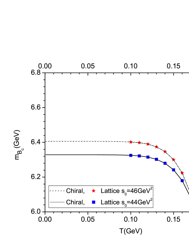
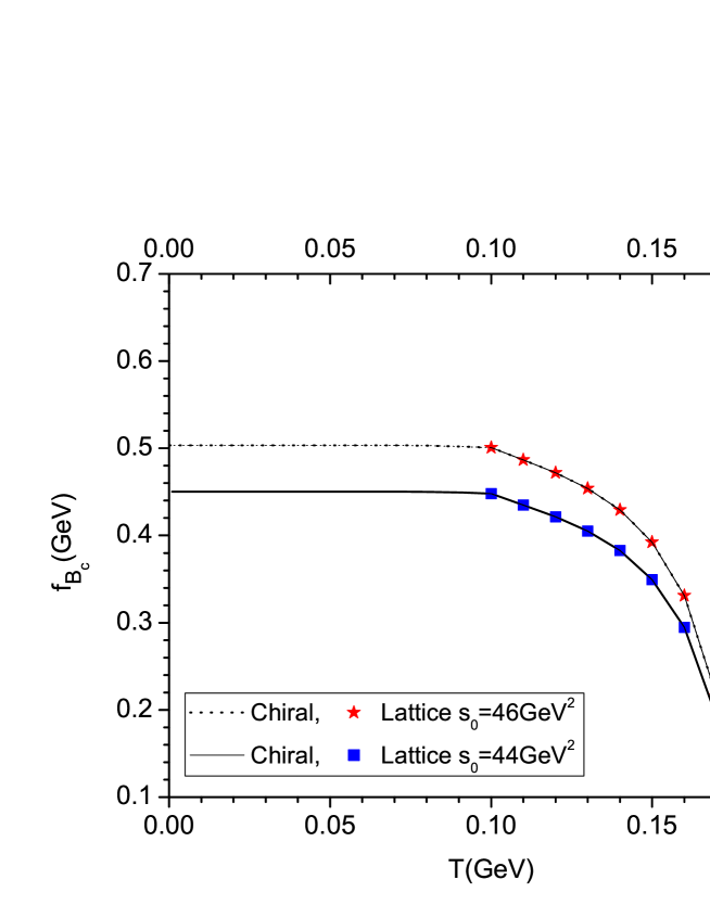
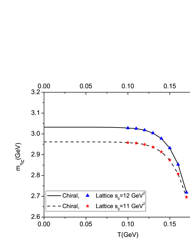
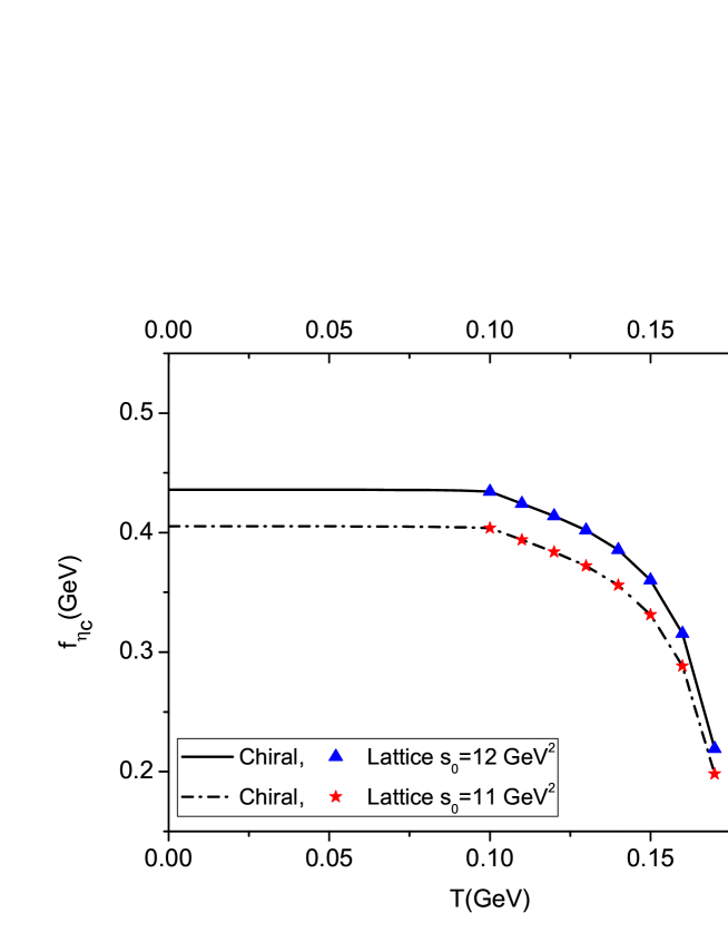
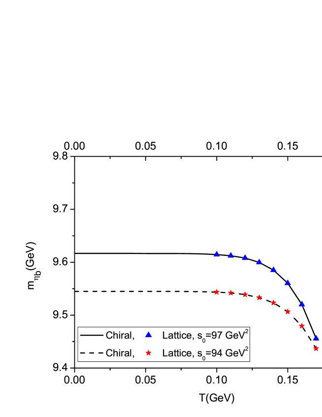
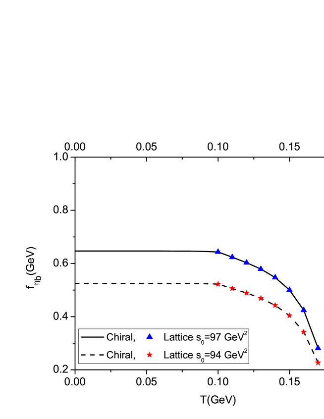
Our calculations show that in the working regions the dependence of the considered observables on auxiliary parameters is weak. We depict the dependence of masses and decay constants on the temperature, $T$ in Figs. 1-6. These figures contain the results obtained using both lattice QCD and chiral perturbation parametrization for the gluonic part of the energy density. These figures depict that both parametrization of lattice QCD and chiral perturbation theory predict the same result in validation limit of lattice QCD fit parametrization, i.e., $0.10~{}GeV\leq T\leq 0.17~{}GeV$. These figures also show that the masses and decay constants remain unchanged approximately up to $T\simeq 100~{}MeV$, but after this point, they start to diminish with increasing the temperature. Near the critical or deconfinement temperature, the decay constants reach approximately to 38% of their values in vacuum, while the masses are decreased about 5%, 10%, 2% comparing with their values at zero temperature for $B_{c}$, $\eta_{c}$, $\eta_{b}$ mesons, respectively. From these figures, we obtain the results on the decay constants and masses at zero temperature as presented in Tables I and II. The quoted errors in these Tables are due to the errors in variation of the continuum threshold at zero temperature, Borel mass parameter as well as errors coming from fit parametrization of the temperature dependent continuum threshold, gluon condensate and strong coupling constant and uncertainties existing in other input parameters. These Tables also include the existing predictions of the other works as well as experimental data. The Table II depicts a very good consistency between our results and the experimental data on masses but from Table I, we see that the present work results and the results existing in the literature (see Table I) on the decay constant are comparable up to presented errors.

Our results for the leptonic decay constants at zero temperature as well as the behavior of the masses and decay constants of the considered pseudoscalar heavy mesons with respect to the temperature can be checked in the future experiments. The obtained behavior of the observables in terms of temperature can be used in analysis of the results of the heavy ion collision experiments.

$$\begin{array}[]{|c|c|c|c|}\hline\cr\hline\cr&f_{B_{c}}(MeV)&f_{\eta_{c}}(MeV)&f_{\eta_{b}}(MeV)\\ \hline\cr\mbox{Present Work}&476\pm 27&421\pm 35&586\pm 61\\ \hline\cr\mbox{QCD sum rules \cite[cite]{\@@bibref{Authors Phrase1YearPhrase2}{V.A.Novikov,T.M.Aliev1,S.S.Gershtein}{\@@citephrase{(}}{\@@citephrase{)}}}}&400\pm 25&350&-\\ \hline\cr\mbox{Potential Model \cite[cite]{\@@bibref{Authors Phrase1YearPhrase2}{V.V.Kiselev}{\@@citephrase{(}}{\@@citephrase{)}}}}&400\pm 45&402&599\\ \hline\cr\mbox{Lattice QCD Method \cite[cite]{\@@bibref{Authors Phrase1YearPhrase2}{TWChiu}{\@@citephrase{(}}{\@@citephrase{)}}}}&489\pm 7&438\pm 11&801\pm 12\\ \hline\cr\mbox{Experiment \cite[cite]{\@@bibref{Authors Phrase1YearPhrase2}{K.W.Edwards}{\@@citephrase{(}}{\@@citephrase{)}}}}&-&335\pm 75&-\\ \hline\cr\hline\cr\end{array}$$

Table 1: Values of the leptonic decay constants of the heavy-heavy pseudoscalar, $B_{c}$, $\eta_{c}$ and $\eta_{b}$ mesons in vacuum. These results have been obtained using the values $M^{2}=15~{}GeV^{2}$, $M^{2}=6~{}GeV^{2}$ and $M^{2}=20~{}GeV^{2}$for $B_{c}$, $\eta_{c}$ and $\eta_{b}$ particles, respectively.

$$\begin{array}[]{|c|c|c|c|}\hline\cr\hline\cr&m_{B_{c}}~{}(GeV)&m_{\eta_{c}}~{}(GeV)&m_{\eta_{b}}~{}(GeV)\\ \hline\cr\mbox{Present Work }&6.37\pm 0.05&2.99\pm 0.04&9.58\pm 0.03\\ \hline\cr\mbox{Experiment \cite[cite]{\@@bibref{Authors Phrase1YearPhrase2}{C.Amsler}{\@@citephrase{(}}{\@@citephrase{)}}}}&6.277\pm 0.006&2.9803\pm 0.0012&9.3909\pm 0.0028\\ \hline\cr\hline\cr\end{array}$$

Table 2: Values of the mass of the heavy-heavy pseudoscalar, $B_{c}$, $\eta_{c}$ and $\eta_{b}$ mesons in vacuum. The same values as Table I for the auxiliary parameters have been used.

IV Acknowledgement

The authors would like to thank T. M. Aliev for his useful discussions. This work is supported in part by the scientific and technological research council of turkey (TUBITAK) under the research project no. 110T284 and research fund of kocaeli university under grant no. 2011/029.

Figure 1: The dependence of the mass of $B_{c}$ meson on temperature for Chiral and Lattice QCD parametrization of the gluonic part of the energy density.

Figure 2: The same as Fig. 1 but for $f_{B_{c}}$.

Figure 3: The same as Fig. 1 but for $m_{\eta_{c}}$.

Figure 4: The same as Fig. 1 but for $f_{\eta_{c}}$.

Figure 5: The same as Fig. 1 but for $m_{\eta_{b}}$.

Figure 6: The same as Fig. 1 but for $f_{\eta_{b}}$.

References

• (1) K. Yagi, T. Hatsuda, Y. Miake, Quark-Gluon Plasma, Cambridge University press (2005).
• (2) J. Letessier, J. Rafelski, Hadrons and Quark-Gluon Plasma, Cambridge University press (2002).
• (3) M.A. Shifman, A. I. Vainstein, V. I. Zakharov, Nucl. Phys. B147, 385 (1979), M.A. Shifman, A.I. Vainstein and V.I. Zakharov, Nucl. Phys. B147, 448 (1979).
• (4) A.I. Bochkarev, M. E. Shaposhnikov, Nucl. Phys. B268, 220 (1986).
• (5) P. Colangelo, A. Khodjamirian, In: At the Frontier of Particle Physics, vol.3, ed. M. Shifman, World Scientific, Singapore, 1495 (2001).
• (6) E.V. Shuryak, Rev. Mod. Phys. 65, 1 (1993).
• (7) T. Hatsuda, Y. Koike, S.H. Lee, Nucl. Phys. B394, 221 (1993); H. G. Dosch, S. Narison, Phys. Lett. B203 (1988) 155.
• (8) S. Mallik, Phys. Lett. B416, 373 (1998).
• (9) S. Mallik, K. Mukherjee, Phys. Rev. D58, 096011 (1998); Phys. Rev. D61, 116007 (2000).
• (10) S. Mallik, A. Nyffeler, Phys. Rev. C63, 065204 (2001).
• (11) E. V. Veliev, J. Phys. G:Nucl. Part. Phys., 35, 035004 (2008); E. V. Veliev, T. M. Aliev, J. Phys. G35, 125002 (2008).
• (12) C.A. Dominguez, M. Loewe, J.C. Rojas, JHEP 08, 040 (2007).
• (13) C. A. Dominguez, M. Loewe, J.C. Rojas, Y. Zhang, Phys. Rev. D81, 014007 (2010).
• (14) E. V. Veliev, G. Kaya, Eur. Phys. J. C63, 87 (2009).
• (15) F. Klingl, S. Kim, S.H. Lee, P. Morath and W. Weise, Phys. Rev. Lett. 82, (1999).
• (16) K. Morita, S. H. Lee, Phys. Rev. C77, 064904 (2008).
• (17) K. Morita, S. H. Lee, Phys. Rev. D82, 054008 (2010).
• (18) E. V. Veliev, H. Sundu, K. Azizi, M. Bayar, Phys. Rev. D82, 056012 (2010).
• (19) V. A. Novikov, L. B. Okun, M. A. Shifman, A. I. Vainshtein and V. I. Zakharov, Phys. Rept. 41, 1 (1978).
• (20) T. M. Aliev, V.L. Eletsky, Sov. J. Nucl. Phys. 38, 936 (1983).
• (21) L. J. Reinders, H. Rubinstein, S. Yazaki, Phys. Rep. 127, 1 (1985).
• (22) I. I. Balitsky, V.M. Braun, A.V. Kolesnichenko, Nucl. Phys. B312, 509 (1989).
• (23) C. A. Dominguez and N. Paver, Phys. Lett. B197, 423 (1987); C. A. Dominguez, N. Paver, Phys. Lett B 318, 629 (1993)..
• (24) S. Narison, Phys. Lett. B210, (1988) 238; Acta Phys. Pol. B 26, 687 (1995).
• (25) T. M. Aliev, O. Yılmaz, Nuovo Cimento A105, 827 (1992); V. V. Kiselev, A.V. Tkabladze, Phys. Rev. D48, 520 (1993).
• (26) P. Ball, V.M. Braun, Phys. Rev. D58, 094016 (1998).
• (27) S. Narison, Phys. Lett. B520, 115 (2001).
• (28) V.V.Kiselev, A.E.Kovalsky, A.I.Onishchenko, Phys. Rev. D64, 054009 (2001), O. Lakhina, arXiv:hep-ph/0612160.
• (29) M. Jamin, B.O. Lange, Phys. Rev. D65, 056005 (2002).
• (30) T. W. Chiu, T. H. Hsieh, C. H. Huang, and K. Ogawa , Phys. Lett. B 651, 171 (2007).
• (31) W. Wang, Y. L. Shen, C. D. Lü, Phys. Rev. D79, 054012 (2009).
• (32) T. M. Aliev, K. Azizi, V. Bashiry, J. Phys. G37, 025001 (2010).
• (33) T. M. Aliev, K. Azizi, M. Savcı, Phys. Lett. B690, 164 (2010).
• (34) A. Das, Finite Temperature Field Theory, Word Scientific (1999).
• (35) M. Cheng, et.al, Phys. Rev. D77, 014511 (2008).
• (36) D. E. Miller, Phys. Rept. 443, 55-96 (2007).
• (37) P. Gerber, H. Leutwyler, Nucl. Phys. B321, 387 (1989).
• (38) O. Kaczmarek, F. Karsch, F. Zantow, P. Petreczky, Phys. Rev. D70, 074505 (2004).
• (39) K. W. Edwards et.al, CLEO Collaboration, Phys. Rev. Lett. 86, 30 (2001).
• (40) C. Amsler et.al (Particle Data Group), Phys. Lett. B667, 1 (2008); K. Nakamura et al. (Particle Data Group), J. Phys. G37, 075021 (2010).
Refer to caption