Quantum Phases of the Planar Antiferromagnetic $\mathbf{J_{1}}$-$\mathbf{J_{2}}$-$\mathbf{J_{3}}$ Heisenberg-Model

Abstract

We present results of a complementary analysis of the frustrated planar $J_{1}$-$J_{2}$-$J_{3}$ spin-1/2 quantum-antiferromagnet. Using dynamical functional renormalization group, high-order coupled cluster calculations, and series expansion based on the flow equation method, we have calculated generalized momentum resolved susceptibilities, the ground state energy, the magnetic order parameter, and the elementary excitation gap. From these we determine a quantum phase diagram which shows a large window of a quantum paramagnetic phase situated between the Néel, spiral and collinear states, which are present already in the classical $J_{1}$-$J_{2}$-$J_{3}$ antiferromagnet. Our findings are consistent with substantial plaquette correlations in the quantum paramagnetic phase. The extent of the quantum paramagnetic region is found to be in satisfying agreement between the three different approaches we have employed.

I Introduction

The search for exotic quantum phases is one of the main interests in the study of spin systems with competing interaction. Ultimately this search may uncover spin liquids (SL) without any magnetic order or long range correlations. En-route however, many interesting quantum paramagnets (QP) lie, which are not magnetically ordered, however exhibit broken spatial symmetries with respect to short range magnetic correlations, either spontaneously or by virtue of the lattice structure, i.e. valence bond crystals (VBC) or solids (VBS). In two dimensions a paradigmatic system in this context is the antiferromagnetic (AFM) $J_{1}$-$J_{2}$ model on the square lattice with frustrating diagonal exchange. As a function of the single parameter $j=J_{2}/J_{1}$ this model is widely accepted to undergo a transition from a Néel state at $j\lesssim 0.4$, to a QP phase for $0.4\lesssim j\lesssim 0.6$ and to a collinear AFM phase beyond that. However, even two decades after first analysis of this Chandra1988 ; Schulz1992 , no consensus has been reached on the nature of the QP phase and the type of transition into it, see e.g. Ref. Richter2010, and references therein. Possible QP phases in the $J_{1}$-$J_{2}$ model include a columnar dimer VBC Read1989 , a plaquette VBC Zhitomirsky1996 , but also a SL Capriotti2001 . For the Néel to VBC transition deconfined quantum criticality has been proposed as a novel scenario Senthil2004 ; rachid08 . Experimentally, the $J_{1}$-$J_{2}$ model may be realized in several layered materials such as Li₂VO(Si,Ge)O₄ LiVO , VOMoO₄ VOMo , and BaCdVO(PO₄)₂ BaCdVO .

One approach to shed additional light on the QP region of the $J_{1}$-$J_{2}$ model is to embed its analysis into a larger parameter space. In this context the $J_{1}$-$J_{2}$-$J_{3}$ model

$$H=J_{1}\sum_{\langle i,j\rangle}{\bf S}_{i}\cdot{\bf S}_{j}+J_{2}\sum_{\langle\langle i,j\rangle\rangle}{\bf S}_{i}\cdot{\bf S}_{j}+J_{3}\sum_{\langle\langle\langle i,j\rangle\rangle\rangle}{\bf S}_{i}\cdot{\bf S}_{j}$$ (1)

has become of renewed interest recently. ${\bf S}_{i}$ refers to spin-$1/2$ operators on the sites of the planar square lattice shown in Fig. 1 a), and $J_{1,2,3}$ are exchange couplings ranging from first, i.e. $\langle i,j\rangle$, up to third-nearest neighbors, i.e. $\langle\langle\langle i,j\rangle\rangle\rangle$. For the remainder of this work we will focus on the AFM case, i.e. $J_{1,2,3}\geq 0$ and set $J_{1}=1$.

Figure 1: a) $J_{1}$-$J_{2}$-$J_{3}$ model. Solid dots refer to lattice sites. Only representative third-nearest-neighbor exchange paths are depicted. b) The classical phase diagram of the $J_{1}$-$J_{2}$-$J_{3}$ model.

Classically, the $J_{1}$-$J_{2}$-$J_{3}$ model allows for four ordered phases Moreo1990 ; Chubukov1991 ; Rastelli1992 ; Ferrer1993 ; Ceccatto1993 , comprising a Néel, a collinear, and two types of spiral states which are depicted in Fig. 1 b). Except for the transition from the diagonal $(q,q)$-spiral to the $(\pi,q)$-spiral state, which is first order, all remaining transitions are continuous. Early analysis of quantum fluctuations Ferrer1993 found the Néel phase to be stabilized by $J_{3}>0$, with the end-point of the classical critical line $J_{3}=1/4-J_{2}/2$ at $J_{2}=0$ shifted to substantially larger values of $J_{3}$. First indications of non-classical behavior for finite $J_{3}>0$ where obtained at $J_{2}=0$. A ’spin-Peierls state’ was found in exact diagonalization (ED) studies in the vicinity of $J_{3}\sim 0.7$, between the Néel phase and the diagonal spiral Leung1996 . Monte-Carlo and $1/N$ expansion resulted in a succession of a VBC and a $Z_{2}$ spin-liquid in this region Capriotti2004 . QP behavior was also conjectured at finite $J_{2},J_{3}$, along the line $J_{2}=2J_{3}$ using Schwinger-Bosons Ceccatto1993 . More recent analysis, based on ED and short-range valence bond methods found an s-wave plaquette VBC, breaking only translational symmetry, along the line $J_{2}+J_{3}=1/2$, up to $J_{2}\lesssim 0.25$ Mambrini2006 . This VBC’s region of stability was then studied by series expansion in the $(J_{2},J_{3})$ plane Arlego2008 . Results from projected entangled pair states (PEPS) at $J_{2}=0$ supported the notion of an s-wave plaquette along the $J_{3}$-axis Murg2009 . However, the symmetry of the QP state remains under scrutiny, since a truncated quantum-dimer model Ralko2009 indicates that the potential plaquette VBC has a subleading columnar dimer admixture in the vicinity of $J_{2}\approx J_{3}\approx 0.25$, similar to ED studies Sindzingre2010 . This implies broken translation and rotation symmetry. For $J_{2}\gtrsim 0.5$, ED shows strong columnar dimer correlations Sindzingre2010 . Finally, the order of the transitions from the QP into the semiclassical phases, and in particular to the diagonal spiral, remain an open issue.

In this work we intend to further clarify the extent of the QP regime, using three complementary techniques, namely, functional renormalization group (FRG), coupled cluster methods (CCM), and series expansion (SE). These methods display rather distinct strengths and limitations which we will combine. CCM and SE are methods which operate inherently in the thermodynamic limit, however require extrapolation with respect to cluster size or expansion order. The FRG method is in principle also formulated in the thermodynamic limit, but its numerical implementation requires one to restrict the spin correlation length to a maximal value, which is much larger than system sizes in ED studies. At present neither of these methods alone allows to investigate the full range of semiclassically ordered and QP states, however their combinations provides completive information on the quantum critical lines bounding QP regions: FRG can signal magnetic instabilities of a paramagnetic state, the SE limits the QP region, and CCM clarifies the stability of part of the ordered states. As a main result of this paper we will show that the quantum critical lines agree remarkably well between all three methods, establishing part of the quantum paramagnetic region rather firmly. Unfortunately none of our approaches allow to determine the symmetry of the QP state unbiased, which leaves this an open issue. The paper is organized as follows. In section II we provide for a brief technical account of all three approaches. Section III is devoted to a discussion of the results. We conclude in section IV.

II Methods

In this work we mainly employ three methods to deal with quantum spin systems, namely FRG, see section II.1, which uses a diagrammatic, dynamical renormalization group approach, CCM, see section II.2, which is a cluster expansion method employing an exponential ansatz for the correlated ground state, and finally SE in the exchange coupling constants, see section II.3, based on continuous unitary transformations. In the following we briefly explain each of these methods.

II.1 Functional Renormalization Group Method

The first approach to tackle the system is based on the functional renormalization group (FRG) in conjunction with a pseudo-fermion representation of the $S=1/2$ spin operators. A detailed description of the FRG in general is given e.g. in Ref. salmhofer01, . For an implementation of FRG with pseudo fermions and an application to the $J_{1}$-$J_{2}$-Heisenberg-model, we refer the reader to Ref. reuther10, . This approach is guided by the idea to treat spin models in the framewok of standard Feynman many body techniques. In order to be able to apply the methods of quantum field theory (Wick’s theorem), we use the pseudo-fermion representation of spin operators,

$$S^{\mu}=\frac{1}{2}\sum_{\alpha\beta}f_{\alpha}^{\dagger}\sigma_{\alpha\beta}^{\mu}f_{\beta}\quad,\quad\alpha,\beta=\uparrow,\downarrow\quad,\quad\mu=x,y,z\;,$$ (2)

where $f_{\uparrow}$ and $f_{\downarrow}$ are the annihilation operators of the pseudo fermions and $\sigma^{\mu}$ are the Pauli-matrices. This representation requires a projection of the larger pseudo-fermion Hilbert space (4 states per lattice site) onto the physical subspace of singly occupied states (2 states). At zero temperature we may perform this projection by putting the chemical potential of the pseudo fermions to zero. Empty or doubly occupied states are acting like a vacancy in the spin lattice and are therefore associated with an excitation energy of order $J$. Quantum spin models are inherently strong coupling models, requiring infinite resummations of perturbation theory. The simplest such approach is mean-field theory of the spin susceptibility, which is known to provide qualitatively correct results in the case that a single type of order is present. On the other hand, frustrated systems are characterized by competing types of order. This is a situation when FRG is a powerful tool, as it allows to resum the contributions in all the different (mixed) channels in a controlled and unbiased way. The first step is the introduction of a sharp infrared frequency cutoff for the Matsubara Green’s functions. FRG then generates a formally exact hierarchy of coupled differential equations for the one-particle-irreducible vertex functions where the frequency cutoff $\Lambda$ is the flow parameter. In Fig. 2 we show the two first equations of the hierarchy, the first one, Fig. 2 (a) for the pseudo-fermion selfenergy, which has a crucial role in particular for highly frustrated interactions (see Ref. reuther10, ), the second one, Fig. 2 (b), for the two-particle vertex function. The $\beta$-function of the latter has a contribution given by the three-particle vertex function. Following Katanin (Ref. katanin, ; salmhofer, ) we approximate the three-particle vertex by the diagram shown in Fig. 2 (c). In this way the random phase approximation (RPA) is recovered as a diagram subset, ensuring the qualitatively correct behavior on the approach to an ordered phase. Another way of saying this is that the conserving properties of the approximation (the Ward identities) are satisfied in a better way. It is worth noting that without the three-particle vertex contribution, RPA cannot be recovered. Keeping the contribution Fig. 2 (c) is formally equivalent to the replacement of the single scale propagator $S^{\Lambda}(i\omega)$ by $-\frac{d}{d\Lambda}G^{\Lambda}(i\omega)$ (where $G^{\Lambda}(i\omega)$ is the scale-dependent Green’s functions). The approximation may be regarded as a natural extension of the usual one-loop truncation, in which all three-particle vertex contributions are discarded. On the other hand it is also important to keep all the terms consisting of two two-particle vertices on the r.h.s. of Fig. 2 (b), as they control disorder tendencies and therefore the size of the paramagnetic region.

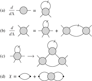
Figure 2: The FRG scheme in diagrammatic form. Lines without a slash represent the Green’s functions and lines with a slash the single-scale propagators. The different vertices are given by circles. The equations (a) and (b) show the FRG flow equations for the selfenergy and the two-particle vertex, respectively. Note that Eq. (b) does not distinguish between the particle-particle channel and the different particle-hole channels. For a full presentation see e.g. Ref. reuther10, . The Katanin truncation scheme is given by the replacement (c). In (d) the relation between the spin-correlation function $\chi$ and the two-particle vertex is displayed.

The FRG equations depicted in Fig. 2 (a)-(c) are solved on the imaginary frequency axis and in real space, rather than in momentum space. The numerical solution requires a discretization on the frequency axis by a logarithmic mesh. We found that it is essential to keep the full frequency dependence of the vertex function (3 frequency variables). The spatial dependence is approximated by keeping correlation functions up to a maximal length. As a result, for each set of discrete frequencies and site indices on external legs of a vertex function, one RG equation is obtained. For well converged results we typically need to keep sets of about $10^{6}$ coupled ordinary differential equations. In the present formulation long-range order (LRO) is not taken into account. Therefore we should not find a stable solution of the equations down to $\Lambda=0$ in the parameter regimes where LRO is present. The existence of a stable solution therefore indicates the absence of LRO. It is worth to emphasize again that our FRG approach has no bias concerning magnetic LRO or a paramagnetic state. Our starting point of free, dispersionless auxiliary fermions does not imply any tendency towards a certain state.

The physical quantities of interest here, the spin susceptibility and spin correlation function may be obtained from the diagrams depicted in Fig. 2 (d). Below we discuss results for the static susceptibilities as a function of the wave vector. In the ordered phases the susceptibility at the $k$-vector corresponding to the magnetic LRO is found to increase as the running cutoff $\Lambda$ is decreased, until the solution becomes unstable below a certain value of $\Lambda$. Thus, the $k$-vector characterizing the magnetic order at hand may be determined as that corresponding to maximal growth of the susceptibility. If the susceptibilities flow smoothly towards $\Lambda=0$ for any $k$-vector, we are in a disordered phase.

II.2 Coupled Cluster Method

Next we analyze the system from a complementary viewpoint using the CCM, the main features of which we briefly illustrate now. For more details the reader is referred to Refs. zeng98, ; krueger01, ; bishop00, ; farnell04, ; rachid05, and references therein. We mention, that the CCM has been applied successfully to determine the stability range of magnetically ordered ground state phases in frustrated quantum magnets krueger01 ; rachid05 ; Schm:2006 ; bishop08 ; bishop08a ; zinke08 ; rachid08 ; richter10 . Moreover, it has been demonstrated that the CCM is appropriate to investigate frustrated quantum spin systems with incommensurate magnetic structures bursill ; krueger01 ; rachid05 ; bishop09 ; zinke09 . The starting point for a CCM calculation is the choice of a normalized reference state $|\Phi\rangle$, together with a set of mutually commuting multispin creation and destruction operators $C_{I}^{+}$ and $C_{I}^{-}$, which are defined over a complete set of many-body configurations $I$. We choose $\{|\Phi\rangle;C_{I}^{+}\}$ in such a way that we have $\langle\Phi|C_{I}^{+}=0=C_{I}^{-}|\Phi\rangle$, $\forall I\neq 0$. Note that the CCM formalism corresponds to the thermodynamic limit $N\rightarrow\infty$. Depending on the model parameters $J_{1}$, $J_{2}$ and $J_{3}$ we have considered the Néel, the collinear, and the diagonal spiral state. Results on the $(\pi,q)$-state could not be obtained at sufficient precision. We work in a locally rotated frame of reference such that all spins of the reference state align along the negative $z$ axis. Obviously, the choice of the rotated coordinate frame depends on the choice of the reference state $|\Phi\rangle$. For a spiral reference state the local rotation angle is related to the pitch $q$. In the rotated coordinate frame the reference state reads $|\Phi\rangle=|\downarrow\rangle|\downarrow\rangle|\downarrow\rangle\ldots\,$, and we can treat each site equivalently. The corresponding multispin creation operators then can be written as $C_{I}^{+}=s_{i}^{+},\,\,s_{i}^{+}s_{j}^{+},\,\,s_{i}^{+}s_{j}^{+}s_{k}^{+},\cdots$, where the indices $i,j,k,\dots$ denote arbitrary lattice sites.

The CCM is based on ket and a bra ground states, $|\Psi\rangle$ and $\langle\tilde{\Psi}|$ respectively, which are parameterized as

$$|\Psi\rangle=e^{S}|\Phi\rangle\ ,\qquad S=\sum_{I\neq 0}{\cal S}_{I}C_{I}^{+}\ ,$$

$$\langle\tilde{\Psi}|=\langle\Phi|\tilde{S}e^{-S}\ ,\qquad\tilde{S}=1+\sum_{I\neq 0}\tilde{\cal S}_{I}C_{I}^{-}\ ,$$ (3)

where the so-called correlation coefficients ${\cal S}_{I}$ and $\tilde{\cal S}_{I}$ are determined from the CCM equations

$$\langle\Phi|C_{I}^{-}e^{-S}He^{S}|\Phi\rangle=0,$$ (4)

$$\langle\Phi|\tilde{\cal S}e^{-S}[H,C_{I}^{+}]e^{S}|\Phi\rangle=0\ ,$$ (5)

for each $I$. Using the Schrödinger equation, $H|\Psi\rangle=E_{0}|\Psi\rangle$, the ground state energy can be written as $E_{0}=\langle\Phi|e^{-S}He^{S}|\Phi\rangle$, whereas the magnetic order parameter is given by $m=-\sum_{i=1}^{N}\langle\tilde{\Psi}|s_{i}^{z}|\Psi\rangle/(Ns)$ , where $s_{i}^{z}$ is expressed in the rotated coordinate frame and $s=1/2$ is the spin quantum number. We note, that for the spiral state the pitch vector $q$ is used as a free parameter in the CCM calculation, which has to be determined by minimization of the CCM ground state energy with respect to $q$.

In order to proceed, the operators $S$ and $\tilde{S}$ have to be truncated approximately. Here we use the well elaborated LSUB$n$ scheme, where only $n$ or fewer correlated spins in all configurations, which span a range of no more than $n$ adjacent (contiguous) lattice sites, are included. The number of fundamental configurations can be reduced exploiting lattice symmetry and conservation laws. In the CCM-LSUB10 approximation we have finally $29\,605$ ($45\,825$) fundamental configurations for the Néel (collinear) reference state and for the CCM-LSUB8 approximation we have finally $20\,876$ fundamental configurations for the spiral reference state.

To obtain results at $n\rightarrow\infty$, the ’raw’ LSUB$n$ data have to be extrapolated. While there are no a-priori rules to do so, a great deal of experience has been gathered for the GS energy and the magnetic order parameter. For the GS energy per spin $E_{0}(n)=a_{0}+a_{1}(1/n)^{2}+a_{2}(1/n)^{4}$ is a reasonable well-tested extrapolation ansatz rachid08 ; krueger01 ; Schm:2006 ; rachid05 ; farnell04 ; bishop00 ; bishop08 ; bishop08a . An appropriate extrapolation rule for the magnetic order parameter for systems showing a GS order-disorder transition is $m(n)=b_{0}+b_{1}(1/n)^{1/2}+b_{2}(1/n)^{3/2}$ with fixed exponents, see Refs. bishop08, ; bishop08a, ; zinke08, ; richter10, . Extrapolations $m(n)=c_{0}+c_{1}(1/n)^{c_{2}}$, with a variable exponent $c_{2}$ have also been employed rachid08 ; Schm:2006 ; rachid05 ; zinke08 .

II.3 Series Expansion

Finally we highlight SE as the third approach which we employ. Our SE for the $J_{1}$-$J_{2}$-$J_{3}$ model will not be carried out on Eq. (1), but on a Hamiltonian which is obtained by a continuous unitary transformation (CUT) Wegner1994 ; Knetter2000 . This transformation is designed such as to pre-diagonalize the Hamiltonian with respect to a discrete ’particle’ number $Q$ which counts the number of excitation quanta within an eigenstate of the unperturbed spectrum. Therefore the SE can be carried out in spaces of fixed $Q$, which greatly reduces the computational complexity as compared to other SE methods. For the latter notions to be of reason, the unperturbed energy spectrum has to be equidistant, which limits the particular types of unperturbed Hamiltonians and phases which can be analyzed. Here we will consider CUT SE results for the $J_{1}$-$J_{2}$-$J_{3}$ model which have been obtained from an unperturbed Hamiltonian which leads to a plaquette VBC ground state. I.e., in contrast to the CCM, the SE starts from the disordered phase. Using a plaquette VBC for this phase is motivated by results from ED, short-range resonating valence bond methods Mambrini2006 ; Sindzingre2010 , and truncated dimer models Ralko2009 which suggest that plaquette correlations in the QP state are dominant for $J_{2}<0.5$. The plaquette VBC will break only translational symmetry. Additional, subleading columnar correlations, which have also been found recently Ralko2009 ; Sindzingre2010 are not included. Some SE results for the phase diagram of the $J_{1}$-$J_{2}$-$J_{3}$ model have been given in Ref. Arlego2008, . Here we extend this analysis by also calculating the ground state energy and by comparison with FRG and CCM. CUT SE using plaquette VBCs has been carried out for various systems recently Arlego2008 ; Arlego2007 ; Arlego2006 ; Brenig2004 ; Brenig2003 ; Brenig2002 and we refer the reader to there, for more details. To start, the Hamiltonian is decomposed into

$$H=H_{0}+H_{1}=\sum_{\bf l}H^{\Box}_{\bf l}(J_{2})+\sum_{{\bf l},{\bf m}}H^{\Box}_{{\bf l},{\bf m}}(J_{1},J_{2},J_{3}),$$ (6)

where the first sum refers to a dense partitioning of the lattice in Fig. 1 a) into disjoint four-spin plaquettes, diagonally crossed by two $J_{2}$ couplings and with $J_{1}$ on the plaquettes set to unity. $H_{0}(J_{2}=0)$ has an equidistant energy spectrum. The second sum contains all inter-plaquette couplings, with $(J_{1},J_{2},J_{3})$ being the expansion parameters of the SE. After the CUT the Hamiltonian reads

$$H_{\mathrm{eff}}=H_{0}+\sum_{k,m,l=1}^{\infty}C_{k,m,l}J_{1}^{k}J_{2}^{m}J_{3}^{l}\,\,,$$ (7)

where each $C_{k,m,l}$ are sums of weighted products of local and inter-plaquette operators $O_{i}^{n}$, which create ($n\geq 0$) and destroy ($n<0$) quanta due to $J_{i}$ within the ladder spectrum of $H_{0}(J_{2}=0)$. The weights are fixed by $H_{0}$ from a set of differential flow-equations Knetter2000 and the $O_{i}^{n}$ are evaluated once for a given topology of exchange couplings $J_{1,2,3}$. We note that for the $J_{1}$-$J_{2}$-$J_{3}$ model we find $|n|\leq 4$. The main point is that the total number of quanta generated by each addend in the sum in Eq. (7) is zero. In turn, the eigenstates are classified by $Q$ and their energy is obtained by diagonalizing $H_{\mathrm{eff}}$ within an $N^{Q}$ dimensional space only, where $N$ is the system size. For the ground state energy $Q=0$ and $N^{Q}\equiv d=1$, which implies that it is given by a single matrix element of $H_{\mathrm{eff}}$, namely $E_{0}=\langle 0|H_{\mathrm{eff}}|0\rangle$, where $|0\rangle$ is the unperturbed bare plaquette state. For one-particle excitations $Q=1$ and $d=N$, which however, due to translational invariance also reduces to $d_{\bf k}=1$, where ${\bf k}$ refers to momentum. Both, the weights and the operators in (7) can be evaluated exactly by arbitrary precision arithmetic codes, leading to analytic results.

III Results

III.1 Ground State Energy

We have used CCM and SE to calculate the ground state energy $E_{0}$ in the ordered and the QP phase, respectively. The ground state energy has also been obtained from ED on 32 sites, both, within the complete Hilbert space and for a nearest neighbor valence-bond basis Mambrini2006 . PEPS calculations have also reported $E_{0}$, however for $J_{2}=0$ only Murg2009 . It is therefore instructive to compare results from these various methods. This is shown in Fig. 3, where we have extended the ED of Ref. Mambrini2006, by calculating more data points and considering also the ordered regimes at $J_{2}=0$. The CCM data in this figure refers to extrapolations using LSUB4-10 (LSUB4-8) in the Néel (spiral) state, as detailed in section II.2. The SE is calculated to $O(5)$ in $J_{2,3}$ and the inter-plaquette $J_{1}$. The complete corresponding analytic expression is to lengthy to be displayed explicitly mailSE , however at $J_{1}$=1 and $J_{2}$=0, as in the figure, it reduces to

$$E_{0} = -\frac{720160379}{1045094400}+\frac{50524391297J_{3}}{87787929600}-\frac{25907023J_{3}^{2}}{34292160}$$ (8)

$$+\frac{2377469J_{3}^{3}}{5598720}-\frac{198439J_{3}^{4}}{1128960}-\frac{1704733J_{3}^{5}}{13547520}$$

The SE result depicted refers to this bare series with no additional extrapolations performed.

First we note that the classical energy, which is not contained in this figure, varies similar with $J_{3}$ as compared to the other graphs plotted, however it is larger by $\sim 0.17J_{1}$ on the average. Secondly, it is obvious that PEPS is significantly higher than the other results Dscaling . This discrepancy is most pronounced in the ordered regimes, where $E_{0}=-0.66953(4)$ is a best currently available value from Quantum Monte-Carlo Kim1998 for the nearest neighbor Heisenberg model. On the other hand, both, CCM and SE are rather close to the ED. Each of them has been plotted up to the critical values $J^{c_{1}}_{3},\ J^{c_{2}}_{3}$ which define the extend of the ordered and QP phases as determined in the following section. At the endpoints CCM and SE match up acceptably, where the agreement at $J^{c_{1}}_{3}$ is best and the convergence of the SE may be less reliable for $J^{c_{2}}_{3}$ which is the larger. Thirdly, having in mind that the finite-size shift of the ED data for $N=32$ is about $+0.01$, see Refs. Richter2010, ; richter10, , it is remarkable that the CCM, ED and SE data almost coincide if $J_{3}$ is not too large. The increase of the difference between the ED and CCM data at larger $J_{3}$ can be attributed to the crossover (i) of the characteristic length scale from nearest-neighbor ($J_{1}$-bonds) to 3rd-nearest-neighbor ($J_{3}$-bonds) separation and (ii) of the characteristic energy scale from $J_{1}$ to $J_{3}$. While the first crossover effect leads to an enhanced finite-size effect in the ED energy and to a larger impact of LSUB$n$ clusters with $n$ beyond those considered here, the second crossover effect automatically enhances any discrepancy of energies roughly proportional to $J_{3}$. Finally we note that, also energies obtained from ED using a restricted nearest neighbor valence-bond basis Mambrini2006 agree very well with those from our CCM, SE, and complete Hilbert space ED.

Figure 3: Ground state energy at $J_{2}=0$: CCM, SE, and ED from this work, nearest-neighbor valence-bond (NNVB) basis from Ref. Mambrini2006, , PEPS from Ref. Murg2009, , and quantum Monte-Carlo (QMC) from Ref. Kim1998, . CCM extrapolation see text. All energies are given in units of $J_{1}$.

III.2 Quantum Phase Diagram

Using FRG the phase diagram has been calculated in the $J_{2}$-$J_{3}$-plane with parameter steps of 0.1 for $0\leq J_{2,3}\leq 1$. A large computational effort is required to solve the system of FRG equations. In the present calculation we used 46 frequency points. The spatial dependence of the susceptibility was kept up to lattice vectors $\mathbf{R}$ satisfying $\textnormal{Max}(|R_{x}|,|R_{y}|)\leq 5$, and the susceptibilities were put to zero beyond that range. This provides a correlation area of $11\times 11$ lattice points, which proved to be sufficient for a first exploration of the phase diagram. The results were then Fourier transformed to momentum space. In magnetic phases we see a pronounced susceptibility peak in momentum space that rapidly grows during the $\Lambda$-flow. At a certain $\Lambda$ the onset of spontaneous LRO is signalled by a sudden stop of the smooth flow and the onset of oscillations depending on the frequency discretization. On the other hand in non-magnetic phases a smooth flow and broad susceptibility peaks are obtained. This distinction allows us to draw the FRG phase diagram of the model, which is shown in Fig. 4. Regarding the error bars in Fig. 4 we note that bars of size 0.1 into the $J_{3}$-direction do not reflect errors of the FRG, but are only due to finite $(J_{2},J_{3})$-spacing and, in principle, apply also to the $J_{2}$-direction. However, especially near the phase boundary between the spiral ordered and the disordered phase, at large $J_{3}$, we encounter enhanced uncertainties. Here $(J_{2},J_{3})$-regions occur where it is not clear if the behavior of the flow should be interpreted as magnetic or non-magnetic. In Fig. 4 these regions lead to error bars larger than 0.1.

Figure 4: Combined quantum phase diagram of the $J_{1}$-$J_{2}$-$J_{3}$ model. Solid: Onset of magnetic flow from FRG on 11$\times$11 sites with 46 frequency points. Error bars of size 0.1 (larger than 0.1) are due to the finite $J_{2,3}$-mesh (uncertainties in the flow of the susceptibility). See text. Dashed: Lines of vanishing order parameter from LSUB$n$ CCM with fixed(variable)-exponent extrapolations from n=4,6,8,10 for diamonds(circles). See text. Dashed-dotted: Triplet-gap closure from 5th-order CUT SE. Small(Large)-$J_{3}$ lines are [3,1]([2,2])-DlogPadé approximants. Shaded region refers to difference between bare series and DlogPadés. ’N’, ’C’, and ’S’ denote Néel, collinear, and spiral state. ’QP’ refers to a generic quantum paramagnet for CCM and FRG and to a plaquette VBC for SE.

To obtain the CCM phase diagram we extrapolate the LSUB$n$ data for the magnetic order parameter $m$, cf. section II.2. Starting in parameter regions where semiclassical magnetic long range order can be supposed we use the classical state as the reference state for the CCM. Then we obtain the phase boundaries of the magnetically ordered phases by determining the lines of vanishing magnetic order parameter $m$, which implies continuous or second order transitions. In Fig. 5 we show typical CCM results for order $m$. For the Néel and the collinear phase we find the extrapolation of $m$ to be nearly independent of the extrapolation scheme used. Unfortunately, for the spiral state, computational constraints limit us to LSUB$n$ with $n\leq 8$. Since the LSUB2 approximation is not appropriate for a proper description at larger $J_{3}$, only 3 CCM data points are left for the extrapolation. In that case we find that the fixed and variable exponent extrapolations lead to rather different critical values for $J_{3}$ at fixed $J_{2}$. Therefore the critical regime of the spiral state cannot be determined accurately enough from the present CCM. This is very different for the ground state energy which allows for stable extrapolation in all three quasiclassical regions. The location of all $J^{c}_{3}(J_{2})$, with $m(J^{c}_{3}(J_{2}))=0$, i.e. the quantum phase diagram as obtained from CCM is included in Fig. 4 for both extrapolation schemes.

Figure 5: Magnetic order parameter $m$ obtained within the CCM-LSUB$n$ approximation as well as extrapolated data using the extrapolation scheme $m(n)=b_{0}+b_{1}(1/n)^{1/2}+b_{2}(1/n)^{3/2}$ and LSUB$n$ data for $n=4,6,8,10$, see Sec.II.2. a) in the Néel phase, b) in the collinear phase.

Finally the phase boundaries have been calculated using SE. To this end the plaquette phase has been analyzed with respect to second order instabilities, i.e., a closure of the elementary triplet gap as a function of $J_{2}$, $J_{3}$. For this, we diagonalize $H_{\mathrm{eff}}$ in the $Q$=1 sector, i.e., the subspace of single-quanta states $|\mathbf{1}\rangle_{\mathbf{l}}$ at sites ${\bf l}$. These states are triplets. The sole action of $H_{\mathrm{eff}}$ on these states is a translation in real space, $H_{\mathrm{eff}}|\mathbf{1}\rangle_{\mathbf{0}}=\sum_{\mathbf{l}}c_{\mathbf{l}}|\mathbf{1}\rangle_{\mathbf{l}}$ with the $c_{\mathbf{l}}$ determined from the SE. Fourier transformation yields the triplet dispersion, similar to a generalized tight-binding problem, with the hopping matrix elements determined from $H_{\mathrm{eff}}$. For technical details we refer to Ref. Arlego2008, . We have used this technique to calculate the triplet dispersion up to 5th order in all three variables $J_{1}$, $J_{2}$ and $J_{3}$. In Fig. 4 we show the resulting lines for the closure of the triplet gaps, as obtained from a Dlog-Padé analysis of this dispersion. The shaded error-region refers to the distance between the critical lines from the bare SE and those from Dlog-Padé and are a measure of convergence of the SE. For $J_{2}\gtrsim 0.5$ the SE’s convergence is insufficient to obtain reliable triplet dispersions.

Figure 4 is a main result of our paper. Most obviously, it shows that within the range of $J_{2,3}$ investigated, the $J_{1}$-$J_{2}$-$J_{3}$ model displays a large QP region. This region extends well beyond the line $J_{2}+J_{3}=1/2$, with $J_{2}\lesssim 0.25$ studied in Ref. Mambrini2006, , or the vicinity of the point $J_{2}\approx J_{3}\approx 0.25$ in Ref. Ralko2009, , and for $J_{2}\lesssim 0.5$ also covers a larger $J_{3}$ interval than that observed in ED Sindzingre2010 . The quantum Néel phase is enlarged with respect to the classical one, which agrees with early 1/S-analysis Ferrer1993 and recent ED resultsSindzingre2010 . Our computational approaches are not capable of an unbiased identification of the symmetry of the QP state. However, since the phase boundaries predicted from the plaquette SE and those from CCM and FRG agree rather well, our results corroborate substantial plaquette correlations in the QP phase for $J_{2}\lesssim 0.3\ldots 0.4$, which is in line with Refs. Mambrini2006, ; Murg2009, ; Ralko2009, ; Sindzingre2010, .

III.3 Short Range Correlations

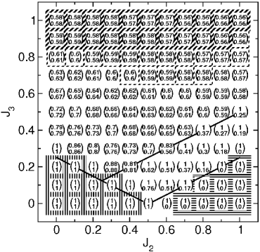
Figure 6: Brackets: wave vector $k_{x}$, $k_{y}$ in units of $\pi$ at maximum of the static susceptibility from FRG. Solid lines indicate the classical critical lines. Vertically, horizontally and diagonally striped frames around the brackets correspond to Néel, collinear, and spiral state, respectively. Thin frames mark regions of uncertain flow behavior.

Since FRG evaluates the static susceptibility over the complete Brillouin zone, it allows to determine the wave vector $\mathbf{k}_{\mathrm{max}}$ of the dominant short-range magnetic correlations or the pitch vector of the magnetic order parameter. These wave vectors are depicted in Fig. 6 together with the quantum phases discussed already in Fig. 4. Both, in the ordered as well as in the QP phase we find the wave vectors at maximum of the susceptibility to agree approximately with those obtained for the purely classical model in Fig. 1 b). This is particularly interesting with respect to the $(\pi,q)$-spiral state, which seems to exist only in the form of short range correlations in Fig. 6.

In order to illustrate how the dominant fluctuations in the disordered phase change with varying couplings, we show in Fig. 7 results for the static susceptibility as a function of the $k$-vector in the Brillouin zone with $k_{x},k_{y}\in[0,\pi]$ at fixed $J_{3}=0.4$ for various values of $J_{2}$. For $J_{2}=0$ we see a broadened peak at a $(q,q)$-position which has already moved away from the Néel-point $\mathbf{k}=(\pi,\pi)$. This peak further moves along the Brillouin-zone diagonal for increasing $J_{2}$. For $J_{2}\gtrsim 0.6$ it is seen that the peak smoothly deforms into an arc and that the weight at the Brillouin-zone boundary increases. Between $J_{2}=0.7$ and $J_{2}=0.8$, close to the classical first order transition, the ridge has constant weight and the maximum jumps to a $(\pi,q)$-direction to then further evolve towards the collinear points $\mathbf{k}=(0,\pi)$, $\mathbf{k}=(\pi,0)$ and to acquire more prominence. Therefore, remnants of the classical correlations survive into the QP regime. Very similar behavior is evidenced by ED Sindzingre2010 .

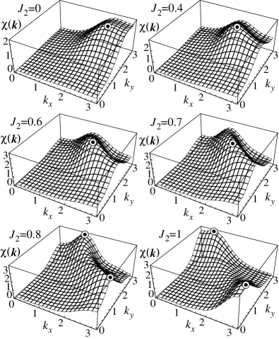
Figure 7: Static susceptibility for wave vectors $k_{x},k_{y}\in[0,\pi]$ for various values $J_{2}$ and constant $J_{3}=0.4$. The black dots mark the positions of the maxima.

IV Conclusion

To summarize, we have studied the quantum phases of the frustrated planar $J_{1}$-$J_{2}$-$J_{3}$ spin-1/2 quantum-antiferromagnet, using FRG, CCM, and CUT SE. This includes evaluations of momentum resolved susceptibilities, the ground state energy, magnetic order parameters, and the elementary excitation gaps. Our results provide clear evidence for a sizeable quantum paramagnetic region which opens up between the Néel, collinear, and spiral state of the purely classical model. A long-range ordered collinear spiral phase, which is also present classically has not been observed in the quantum model in the parameter range we have investigated. Where applicable, the agreement between the critical lines determined from all three methods is remarkably good. While our computational approaches cannot determine potentially broken symmetries in the quantum paramagnetic state, the fact that the critical lines which we have obtained from FRG and CCM agree well with those from the CUT SE which is based on a plaquette VBC, is indicative of VBC ordering with substantial plaquette correlations in the quantum paramagnetic region - in those parameter ranges where CUT SE applies. Our results are consistent with second order transitions from the Néel and the collinear state into the quantum paramagnet. Unexpectedly, our CCM results do not provide a definite signal of a transition from the spiral state into the quantum paramagnet. This may simply be related to an insufficient order of the LSUBn approximation, but could also hint at a first order transition and an intermediate phase between the VBC and the spiral state. Finally, while our findings do not show a collinear spiral state as in the classical model, FRG convincingly demonstrates that the latter is replaced by corresponding short range correlations in the quantum paramagnetic region.

V Acknowledgments

J. Reuther and P. Wölfle acknowledge support through the DFG research unit FOR 960 ”Quantum phase transitions”. M. Arlego and W. Brenig acknowledge partial support by the CONICET through grant 2049/09 and the DFG through grant 444 ARG-113/10/0-1. J. Richter and W. Brenig thank the Max-Planck-Institute for Physics of Complex Systems for its hospitality during the Advanced Study Group ”Unconventional Magnetism in High Fields” where part of this work was completed.

References

- (1) P. Chandra and B. Doucot, Phys. Rev. B 38, 9335 (1988)
- (2) H. J. Schulz and T. A. L. Ziman, Europhys. Lett. 18, 355 (1992)
- (3) J. Richter and J. Schulenburg, Eur. Phys. J. B 73, 117 (2010)
- (4) N. Read and S. Sachdev, Phys. Rev. Lett. 62, 1694 (1989).
- (5) M. E. Zhitomirsky and K. Ueda, Phys. Rev. B 54, 9007 (1996)
- (6) L. Capriotti, F. Becca, A. Parola, and S. Sorella, Phys. Rev. Lett. 87, 097201 (2001)
- (7) T. Senthil, A. Vishwanath, L. Balents, S. Sachdev, and M. P. A. Fisher, Science 303, 1490 (2004)
- (8) R. Darradi, O. Derzhko, R. Zinke, J. Schulenburg, S.E. Krüger and J. Richter, Phys. Rev. B 78, 214415(2008).
- (9) R. Melzi, P. Carretta, A. Lascialfari, M. Mambrini, M. Troyer, P. Millet, and F. Mila, Phys. Rev. Lett. 85, 1318 (2000); P. Carretta, R. Melzi, N. Papinutto, and P. Millet, ibid. 88, 047601 (2002); H. Rosner, R.R.P. Singh, W. H. Zheng, J. Oitmaa, S.-L. Drechsler, and W. Pickett, ibid. 88, 186405 (2002); A. Bombardi, J. Rodriguez-Carvajal, S. Di Matteo, F. de Bergevin, L. Paolasini, P. Carretta, P. Millet, and R. Caciuffo, ibid. 93, 027202 (2004).
- (10) P. Carretta, N. Papinutto, C. B. Azzoni, M. C. Mozzati, E. Pavarini, S. Gonthier, and P. Millet, Phys. Rev. B 66, 094420 (2002)
- (11) R. Nath, A. A. Tsirlin, H. Rosner, and C. Geibel, Phys. Rev. B 78, 064422 (2008).
- (12) A. Moreo, E. Dagotto, Th. Jolicoeur, and J. Riera, Phys. Rev. B 42, 6283 (1990)
- (13) A. Chubukov, Phys. Rev. B 44, 392 (1991)
- (14) E. Rastelli and A. Tassi, Phys. Rev. B 46, 10793 (1992)
- (15) J. Ferrer, Phys. Rev. B 47, 8769 (1993)
- (16) H. A. Ceccatto, C. J. Gazza, and A. E. Trumper, Phys. Rev. B 47, 12329 (1993)
- (17) P. W. Leung and N.W. Lam Phys. Rev. B 53, 2213 (1996)
- (18) L. Capriotti, and S. Sachdev, Phys. Rev. Lett. 93, 257206 (2004)
- (19) M. Mambrini, A. Lauechli, D. Poilblanc, and F. Mila, Phys. Rev. B 74, 144422 (2006)
- (20) M. Arlego and W. Brenig, Phys. Rev. B 78, 224415 (2008)
- (21) V. Murg, F. Verstraete, and J. Cirac, Phys. Rev. B 79, 195119 (2009)
- (22) A. Ralko, M. Mambrini, and D. Poilblanc, Phys. Rev. B 80, 184427 (2009)
- (23) P. Sindzingre, N. Shannon, and T. Momoi, J. Phys.: Conf. Ser. 200, 022058 (2010)
- (24) M. Salmhofer and C. Honerkamp, Prog. Theor. Phys. 105, 1 (2001).
- (25) J. Reuther and P. Wölfle, Phys. Rev. B 81, 144410 (2010).
- (26) A. A. Katanin, Phys. Rev. B 70, 115109 (2004).
- (27) M. Salmhofer, C. Honerkamp, W. Metzner, and O. Lauscher, Prog. Theor. Phys. 112, 943 (2004).
- (28) C. Zeng, D. J. J. Farnell, and R. F. Bishop, J. Stat. Phys. 90, 327 (1998).
- (29) S. E. Krüger and J. Richter, Phys. Rev. B 64, 024433 (2001).
- (30) R. F. Bishop, D. J. J. Farnell, S. E. Krüger, J. B. Parkinson, and J. Richter, J. Phys.: Condens. Matter 12, 6877 (2000).
- (31) D. J. J. Farnell and R. F. Bishop, in: Quantum Magnetism, eds. U. Schollwöck, J. Richter, D. J. J. Farnell, and R. F. Bishop, Lecture Notes in Physics 645 (Springer, Berlin, 2004), p. 307.
- (32) R. Darradi, J. Richter, and D. J. J. Farnell, Phys. Rev. B 72, 104425 (2005).
- (33) D. Schmalfuß, R. Darradi, J. Richter, J. Schulenburg, and D. Ihle, Phys. Rev. Lett. 97, 157201 (2006).
- (34) R. F. Bishop, P. H. Y. Li, R. Darradi, and J. Richter, J. Phys.: Condens. Matter 20, 255251 (2008).
- (35) R. F. Bishop, P. H. Y. Li, R. Darradi, J. Schulenburg, and J. Richter, Phys. Rev. B 78, 054412 (2008).
- (36) R. Zinke, J. Schulenburg, and J. Richter, Eur. Phys. J. B 64, 147 (2008).
- (37) J. Richter, R. Darradi, J. Schulenburg, D.J.J. Farnell, and H. Rosner, Phys. Rev. B 81, 174429 (2010).
- (38) R. Bursill, G.A. Gehring, D.J.J. Farnell, J.B. Parkinson, T. Xiang, and C. Zeng, J. Phys.: Condens. Matter 7, 8605 (1995).
- (39) R.F. Bishop, P.H.Y. Li, D. J. J. Farnell, and C.E. Campbell, Phys. Rev. B 79, 174405 (2009).
- (40) R. Zinke, S.-L. Drechsler and J. Richter, Phys. Rev. B 79, 094425 (2009).
- (41) F.J. Wegner, Ann. Phys. 3, 77 (1994).
- (42) C. Knetter and G.S. Uhrig, Eur. Phys. J. B 13, 209 (2000).
- (43) M. Arlego and W. Brenig, Phys. Rev. B 75, 024409 (2007).
- (44) M. Arlego and W. Brenig, Eur. Phys. J. B 53, 193 (2006).
- (45) W. Brenig and M. Grzeschik, Phys. Rev. B 69, 064420 (2004).
- (46) W. Brenig, Phys. Rev. B 67, 064402 (2003).
- (47) W. Brenig and A. Honecker, Phys. Rev. B 65, 140407(R) (2002).
- (48) The complete SE for will be made available by email from the authors upon request.
- (49) Figure 3 displays PEPS with local dimension . The improvement over (see Ref. Murg2009, ) is small on the -scale of Fig. 3. This may suggest rather large values of to be necessary to improve PEPS.
- (50) J.-K. Kim and M. Troyer, Phys. Rev. Lett. 80, 2705 (1998)