$d^{0}$ Perovskite-Semiconductor Electronic Structure

Abstract

We address the low-energy effective Hamiltonian of electron doped $d^{0}$ perovskite semiconductors in cubic and tetragonal phases using the $\bm{k\cdot p}$ method. The Hamiltonian depends on the spin-orbit interaction strength, on the temperature-dependent tetragonal distortion, and on a set of effective-mass parameters whose number is determined by the symmetry of the crystal. We explain how these parameters can be extracted from angle resolved photo-emission, Raman spectroscopy, and magneto-transport measurements and estimate their values in SrTiO₃.

I Introduction

Transition metal oxides with perovskite structures exhibit a wide variety of interesting and often useful effects including colossal magnetoresistance,CMR high $T_{c}$ superconductivity,highTcSC and ferroelectricityferroelectricity . Correspondingly, these materials have received intense experimental and theoretical attention for over half a centurygoodenough . Within the perovskite family, the $d^{0}$ materials have received particular attention, often because of their large band gaps. SrTiO₃, for example, is perhaps the most common substrate for the epitaxial growth of oxide materials. Recently there has been growing interest in the transport properties of lightly electron doped $d^{0}$ perovskites.HighMobilitySTO In KTaO₃, for example, strong spin-orbit (SO) coupling facilitates electrical manipulation of spin in a field effect transistor geometry.KTO The two-dimensional electron systems which form at interfaces between $d^{0}$ materialsLAO_STO_Hwang show intriguing magnetic phasesLAO_STO_magnetic and peculiar magneto-transport features.Dagan ; LiorKlein Advanced epitaxial growth techniques enable $\delta$-doping of oxidesdeltaDopedSTO and the fabrication of oxide hetrostructures.hetrostructures These relatively recent rapid advances could, it is hoped, eventually lead to useful oxide based nano-electronic devices.enterOxides

The low-energy band structure of an oxide provides a starting point for understanding not only its bulk transport characteristics but also its electronic properties near $\delta$-doped layers and near interfaces. First principles electronic structure theory methodsMattheiss1 ; Mattheiss2 ; KTOnumerics are usually efficient for determining the gross structure of a band, but are not sufficiently accurate to nail down the fine features that determine the electronic properties of the states at the bottom of the conduction band that are important in weakly doped bulk materials, and in low-carrier-density two-dimensional electron systems. In particular, it appears that at present bulk band structures in $d^{0}$ perovskites are not known accurately enough to predict the two-dimensional bands of $\delta$-doped oxides or of interface-localized bands in oxide based hetrostructures. This paper is primarily motivated by the goal of assisting progress in this direction.

The $\bm{k\cdot p}$ methodDresselhaus ; cardona offers an alternative and a potentially more accurate route for characterizing band structure near the conduction band minimum. The method provides an effective Hamiltonian that depends on a set of phenomenological parameters which can be small in number when band extrema occur at high-symmetry points in momentum space. The utility of this method hinges on the ability to extract accurate parameter values from experiments. In the case of perovskites the most valuable experimental probes are angle resolved photo-emission (ARPES), Raman spectroscopy, and magneto-transport measurements.

Many of the most studied oxides have conduction-band minima located at the center of the Brillioun zone. We therefore apply the $\bm{k\cdot p}$ method to obtain an effective low energy Hamiltonian near the $\Gamma$ point. At high temperatures, perovskites typically have cubic symmetry. As the temperature is decreased the symmetry is usually lowered, most commonly to either orthorhombic or tetragonal. The distortion can be driven by the motion of atoms along one of the cubic axes (e.g. in BaTiO₃) or by a rotation of the oxygen octahedras (e.g. in SrTiO₃). Structural phase transitions can also be induced by applied stress.expitaxialStressSTO

In this work we focus on the cubic and tetragonal phases. In section II we briefly describe the $\bm{k\cdot p}$ method and then use it to derive the low energy effective theory of a $d^{0}$ perovskite in the vicinity of the $\Gamma$ point. In section III we elaborate on experimental methods for obtaining the parameters of the $\bm{k\cdot p}$ Hamiltonian. Using the experimental data accumulated over the past few decades we then study the effective Hamiltonian of the conduction bands of SrTiO₃ in Section IV. We summarize in section V.

II Low energy theory

For many perovskites of current interest such as SrTiO₃ the conduction band minima is at the Brillouin-zone center $\Gamma$-point. For momenta near the $\Gamma$-point the crystal field splits the ten $d$-bands into four high energy $e_{g}$ bands, and six lower energy $t_{2g}$ bands. Because the crystal field induced gap is typically a few eV’s, it is sufficient to consider the $t_{2g}$ bands when constructing a low energy theory of weakly-doped $d^{0}$ materials. In the cubic phase the $t_{2g}$ bands are degenerate at the $\Gamma$-point if spin-orbit interactions are neglected, but are weakly-split by typical tetragonal or orthorhombic distortions and by weak spin-orbit interactions. Unless the Fermi energy is large compared to these splittings, spin-orbit and distortion related band parameters must be accurately known in order to achieve a reasonable description of electronic properties.

II.1 Effective Hamiltonian

The unperturbed Hamiltonian in the $\bm{k\cdot p}$ perturbation theoryDresselhaus ; cardona is

$$H_{0}=\frac{p^{2}}{2m}+V(\bm{r})+\frac{\hbar}{4m^{2}c^{2}}\left(\nabla V\times\bm{p}\right)\cdot\sigma.$$ (1)

$H_{0}$ consists of three terms: the kinetic energy term, the lattice potential term $V(\bm{r})$, and the spin-orbit term ($\sigma$ is the Pauli matrix vector). The $\bm{k\cdot p}$ Hamiltonian, which acts on the periodic part of the Bloch state, includes a second term which accounts for the dependence of band wavefunctions on Bloch wavevector $\bm{k}$:

$$H_{\bm{k\cdot p}}=\frac{\bm{k}}{m}\cdot\left(\bm{p}+\frac{1}{4m^{2}c^{2}}\bm{\sigma}\times\nabla V\right)\equiv\frac{\bm{k}}{m}\cdot\bm{P}.$$ (2)

The $\bm{k\cdot p}$ method exploits the high symmetry at the $\Gamma$ point to classify the $\bm{k}=0$ wave functions by irreducible representations (irreps) of the appropriate point group symmetry. It then uses perturbation theory

$$h_{ij}=\delta_{ij}k^{2}+\sum_{\alpha}\frac{\langle\psi_{i}|H_{\bm{k\cdot p}}|\phi_{\alpha}\rangle\langle\phi_{\alpha}|H_{\bm{k\cdot p}}|\psi_{j}\rangle}{E_{i}(0)-E_{\alpha}(0)}$$ (3)

to evaluate $t_{2g}$ projected Hamiltonian corrections to second order in the Bloch wavevector $\bm{k}$. Hereafter we use units in which $\hbar=2m=1$ where $m$ is the bare mass of the electron. The six $t_{2g}$ band energies $\epsilon(\bm{k})$ then follow from the secular equation

$$\det[h_{\mbox{\tiny SO}}+h_{\mbox{\tiny L}}+h(\bm{k})-\epsilon(\bm{k})I]=0.$$ (4)

In Eq.(3) $\{|\psi_{j}\rangle\}$ label a basis set for the $t_{2g}$ bands and $\phi_{\alpha}$ is summed over bands outside the $t_{2g}$ manifold. The first order term was omitted in Eq.(3) since it vanishes for the perovskite structure by inversion symmetry. The matrices $h_{\mbox{\tiny L}}$ and $h_{\mbox{\tiny SO}}$ account phenomenologically for tetragonal distortion and SO interactions at the $\Gamma$ point and are discussed more explicitly below.

The wave functions at the zone center have no covalent character and can be spanned by the $t_{2g}$ basis

$$\{X_{\uparrow},Y_{\uparrow},Z_{\uparrow},X_{\downarrow},Y_{\downarrow},Z_{\downarrow}\}.$$ (5)

Here $X,Y$ and $Z$ correspond respectively to the $|yz\rangle,|xz\rangle$ and $|xy\rangle$ $t_{2g}$ orbitals. Below we obtain the Hamiltonian matrix in this basis.

The lattice term $h_{\mbox{\tiny L}}$ is non zero in the tetragonal phase. If we choose a convenient zero of energy and set the $\bm{\hat{z}}$ axis along the tetragonal axis then $h_{\mbox{\tiny L}}$ has a single non-zero matrix element:

$$\langle Z\alpha|V|Z\alpha\rangle=\Delta_{\mbox{\tiny T}},$$ (6)

where $\alpha$ accounts for the spin. The SO term in the Hamiltonian is

$$\left(h_{\mbox{\tiny SO}}\right)_{i\alpha,k\beta}=\langle\xi_{i}\alpha|\Lambda\cdot\sigma|\xi_{k}\beta\rangle=\langle\xi_{i}|\Lambda_{j}|\xi_{k}\rangle\cdot\langle\alpha|\sigma_{j}|\beta\rangle,$$ (7)

where $\Lambda\propto\nabla V\times\bm{p}$ and $\xi_{i}$ is one of the orbital basis functions. Because $\Lambda$ transforms as a pseudovector, $\langle\xi_{i}|\Lambda_{j}|\xi_{k}\rangle\propto\epsilon_{ijk}$ where $\epsilon_{ijk}$ is the third rank antisymmetric tensor. For example, $\langle X|\Lambda_{z}|X\rangle$ and $\langle X|\Lambda_{z}|Z\rangle$ vanish under reflection off the x-z plane. Furthermore, since the matrix elements (7) must be imaginary

$$\langle\xi_{i}|\Lambda_{j}|\xi_{k}\rangle=-i\frac{\Delta_{\mbox{\tiny SO}}}{3}\epsilon_{ijk}.$$ (8)

Strictly speaking, SO coupling is described by two parameters in the tetragonal phase. However we neglect this small correction since it is of order of $\Delta_{\mbox{\tiny T}}$ over the band gap compared to the spin-orbit coupling term we retain.

The $\bm{k}$-dependent part of the Hamiltonian $h$ is obtained using Eq.(3). We show in the appendix A that

$$h=\left(\begin{array}[]{cc}h_{\uparrow}&0\\ 0&h_{\downarrow}\\ \end{array}\right)$$ (9)

with

$$h_{\alpha}=\left(\begin{array}[]{ccc}{\cal L}_{5}k_{x}^{2}+{\cal M}_{5}^{\parallel}k_{y}^{2}+{\cal M}_{5}^{\perp}k_{z}^{2}&{\cal N}_{5}k_{x}k_{y}&{\cal N}_{45}^{\star}k_{x}k_{z}\\ {\cal N}_{5}k_{x}k_{y}&{\cal L}_{5}k_{y}^{2}+{\cal M}_{5}^{\parallel}k_{x}^{2}+{\cal M}_{5}^{\perp}k_{z}^{2}&{\cal N}_{45}^{\star}k_{y}k_{z}\\ {\cal N}_{45}k_{x}k_{z}&{\cal N}_{45}k_{y}k_{z}&{\cal M}_{4}(k_{x}^{2}+k_{y}^{2})+{\cal L}_{4}k_{z}^{2}\end{array}\right)|\alpha\rangle.$$ (10)

In the tetragonal phase the $h$ matrix depends on eight real parameters (only ${\cal N}_{45}$ may be complex). In the cubic phase parameter values become independent of their subscript labels (e.g. ${\cal L}_{4}={\cal L}_{5}\to L$) and $h$ then depends on only three parameters. The energy dispersion relations follow from Eqs.(4,6—10). Because the Hamiltonian is time-reversal invariant and has inversion symmetry it gives rise to three doubly-degenerate bands.

In the next section we discuss zone-center wave functions and energies. The wavefunctions play a crucial role in matrix-element considerations which powerfully expand the ability of ARPES experiments to determine the parameters of the $\bm{k\cdot p}$-Hamiltonian. The zone-center energies can be compared with $t_{2g}$ band-splitting values obtained by Raman spectroscopy.

II.2 Zone center energies and wave-functions

The Hamiltonian at the zone center is $h_{\mbox{\tiny L}}+h_{\mbox{\tiny SO}}$. The energies are therefore

$$\epsilon_{6} = 0$$

$$\epsilon^{(a)}_{7} = \frac{\Delta_{\mbox{\tiny SO}}}{2}+\frac{\Delta_{\mbox{\tiny T}}}{2}-\frac{Q}{3}$$

$$\epsilon^{(b)}_{7} = \frac{\Delta_{\mbox{\tiny SO}}}{2}+\frac{\Delta_{\mbox{\tiny T}}}{2}+\frac{Q}{3},$$

where

$$Q=\frac{3}{2}\sqrt{\Delta_{\mbox{\tiny SO}}^{2}-\frac{2}{3}\Delta_{\mbox{\tiny SO}}\Delta_{\mbox{\tiny T}}+\Delta_{\mbox{\tiny T}}^{2}}.$$ (12)

(Energy has been shifted so that $\epsilon_{6}$ will vanish.) In the cubic phase the $t_{2g}$ bands transform as $\Gamma^{+}_{25}$ in the absence of spin-orbit coupling. SO interactions split the bands to $\Gamma_{7}^{+}+\Gamma_{8}^{+}$. When there is a tetragonal transition, the four-fold degenerate $\Gamma_{8}$ states further split to $\Gamma_{7}+\Gamma_{6}$. The notation in Eqs.(LABEL:E_tetragonal) correspond to these latter irreps.

The (unnormalized) wave functions corresponding to the energies (LABEL:E_tetragonal) are

$$\psi^{6}_{1} = X_{\downarrow}-iY_{\downarrow}$$

$$\psi^{6}_{2} = X_{\uparrow}+iY_{\uparrow}$$

$$\psi^{7a}_{1} = (Q+D)X_{\uparrow}-i(Q+D)Y_{\uparrow}+2\Delta_{\mbox{\tiny SO}}Z_{\downarrow}$$

$$\psi^{7a}_{2} = \Delta_{\mbox{\tiny SO}}X_{\downarrow}+i\Delta_{\mbox{\tiny SO}}Y_{\downarrow}-(Q-D)Z_{\uparrow}$$

$$\psi^{7b}_{1} = (Q-D)X_{\uparrow}-i(Q-D)Y_{\uparrow}-2\Delta_{\mbox{\tiny SO}}Z_{\downarrow}$$

$$\psi^{7b}_{2} = \Delta_{\mbox{\tiny SO}}X_{\downarrow}+i\Delta_{\mbox{\tiny SO}}Y_{\downarrow}+(Q+D)Z_{\uparrow}$$ (13)

where

$$D=3\Delta_{\mbox{\tiny T}}/2-\Delta_{\mbox{\tiny SO}}/2.$$ (14)

It is interesting to follow the evolution of the bands as the ratio between $\Delta_{\mbox{\tiny T}}$ and $\Delta_{\mbox{\tiny SO}}$ is varied from zero to infinity. The two limits are given in table 1. In the cubic phase the states $\{\psi^{6},\psi^{7a}\}$ are degenerate and are spilt off from the $\{\psi^{7b}\}$ states by an energy of $\Delta_{\mbox{\tiny SO}}$. In the tetragonal phase when $|\Delta_{\mbox{\tiny SO}}|>|\Delta_{\mbox{\tiny T}}|$ the states group to the three doubly degenerate pairs $\psi^{6},\psi^{7a}$ and $\psi^{7b}$. As the temperature is lowered the four $\psi^{7}$ states mix. If eventually $|\Delta_{\mbox{\tiny SO}}|\ll|\Delta_{\mbox{\tiny T}}|$ then the $\psi^{7a}_{1}$ and $\psi^{7b}_{1}$ states combine to give the $Z_{\downarrow}$ state which is purely tetragonal in character.

$\Delta_{\mbox{\tiny T}}=0$	$\Delta_{\mbox{\tiny SO}}=0$
$\left(X_{\downarrow}-iY_{\downarrow}\right),\Gamma_{6}(\Gamma_{8})$	$\left(X_{\downarrow}-iY_{\downarrow}\right),\Gamma_{6}(\Gamma_{5})$
$\left(X_{\uparrow}+iY_{\uparrow}\right),\Gamma_{6}(\Gamma_{8})$	$\left(X_{\uparrow}+iY_{\uparrow}\right),\Gamma_{6}(\Gamma_{5})$
$\left[X_{\uparrow}-iY_{\uparrow}+2Z_{\downarrow}\right],\Gamma_{7}(\Gamma_{8})$	$Z_{\downarrow},\Gamma_{7}(\Gamma_{4})$
$\left[X_{\downarrow}+iY_{\downarrow}-2Z_{\uparrow}\right],\Gamma_{7}(\Gamma_{8})$	$-Z_{\uparrow},\Gamma_{7}(\Gamma_{4})$
$\left[-X_{\uparrow}+iY_{\uparrow}+Z_{\downarrow}\right],\Gamma_{7}$	$-\left(X_{\uparrow}-iY_{\uparrow}\right),\Gamma_{7}(\Gamma_{5})$
$\left[X_{\downarrow}+iY_{\downarrow}+Z_{\uparrow}\right],\Gamma_{7}$	$\left(X_{\downarrow}+iY_{\downarrow}\right),\Gamma_{7}(\Gamma_{5})$

Table 1: Zone center wave functions in the cubic phase with SO interactions (left column) and in the tetragonal phase in the absence of SO interactions (right column).

In the following section we discuss energy dispersion relations along symmetry lines and planes, which can be directly related to ARPES measurements and enable some qualitative insights into the relationships between Hamiltonian parameters and the field-orientation dependence of magnetoresistance-oscillation frequencies.

II.3 Energy dispersion relations for high-symmetry lines and planes

In general Eq.(4) must be diagonalized numerically. However, simple energy dispersion relations exist along high symmetry directions and in high-symmetry planes.

When the tetragonal distortion is large and SO interactions can be neglected, the $t_{2g}$ bands split into $\Gamma_{4}+\Gamma_{5}$ bands. In this limit (to order $k^{4}/\Delta_{\mbox{\tiny T}}$)

$$\epsilon_{4}(\bm{k}) = \Delta_{\mbox{\tiny T}}+{\cal M}_{4}k_{\parallel}^{2}+{\cal L}_{4}k_{z}^{2}$$

$$\epsilon_{5\pm}(\bm{k}) = {\cal B}_{+}k_{\parallel}^{2}+{\cal M}_{5}^{\perp}k_{z}^{2}$$

$$\pm \sqrt{{\cal B}_{-}k_{\parallel}^{4}-4\left[{\cal B}_{-}^{2}-{\cal N}_{5}^{2}\right]k_{x}^{2}k_{y}^{2}}$$

where $k_{\parallel}^{2}=k_{x}^{2}+k_{y}^{2}$ and ${\cal B}_{\pm}=({\cal L}_{5}\pm{\cal M}_{5}^{\parallel})/2$. To leading order in $\Delta_{\mbox{\tiny SO}}$, the $\Gamma_{4}$ energies remain unchanged whereas the $\Gamma_{5\pm}$ energies vary linearly in opposite directions. The energies (II.3) are valid for any value of $\Delta_{\mbox{\tiny T}}$ (but still neglecting $\Delta_{\mbox{\tiny SO}}$) in the $k_{z}=0$ plane. Similarly for the $k_{y}=0$ plane

$$\epsilon_{5-}(\bm{k}) = {\cal M}_{5}^{\parallel}k_{x}^{2}+{\cal M}_{5}^{\perp}k_{z}^{2}$$

$$\epsilon_{4,5+}(\bm{k}) = \frac{\Delta_{\mbox{\tiny T}}}{2}+\frac{{\cal M}_{4}+{\cal L}_{5}}{2}k_{x}^{2}+\frac{{\cal L}_{4}+{\cal M}_{5}^{\perp}}{2}k_{z}^{2}$$ (16)

$$\pm \frac{1}{2}\bigg{(}\left[\Delta_{\mbox{\tiny T}}+\left({\cal M}_{4}-{\cal L}_{5}\right)k_{x}^{2}+\left({\cal L}_{4}-{\cal M}_{5}^{\perp}\right)k_{z}^{2}\right]^{2}$$

$$+4|{\cal N}_{45}|^{2}k_{x}^{2}k_{z}^{2}\bigg{)}^{1/2}.$$

The $\bm{k\cdot p}$ Hamiltonian for the $t_{2g}$ bands in the cubic phase is identical to that of the valence band p-states of zinc-blende type semiconductors.Dresselhaus ; cardona In the presence of moderate SO interactions the dispersion relations along the three equivalent principle axes are

$$\epsilon_{7}(k) = Mk^{2}$$

$$\epsilon_{8\pm}(k) = {\cal B}_{+}k^{2}+\frac{\Delta_{\mbox{\tiny SO}}}{2}$$

$$\pm \sqrt{{\cal B}_{-}^{2}k^{4}+\left(\frac{\Delta_{\mbox{\tiny SO}}}{2}\right)^{2}-\frac{\Delta_{\mbox{\tiny SO}}}{3}{\cal B}_{-}k^{2}}.$$

For strong SO interactions the $\psi^{7}$ and $\psi^{8}$ states can be approximately decoupled to order $k^{4}/\Delta_{\mbox{\tiny SO}}$. The energy dispersions are then

$$\epsilon_{7}(k) = \Delta_{\mbox{\tiny SO}}+Ak^{2}$$ (18)

$$\epsilon_{8}(\bm{k}) = Ak^{2}\pm\sqrt{B^{2}k^{4}+C^{2}(k_{x}^{2}k_{y}^{2}+k_{x}^{2}k_{z}^{2}+k_{y}^{2}k_{z}^{2})}$$

where $A=1+(L+2M)/3$, $B=(L-M)/3$, and $C^{2}=\left[N^{2}-(L-M)^{2}\right]/3$. Expressions (18) were obtained by Dresselhaus et. al.[Dresselhaus, ].

ARPES measurements are frequently set to measure the energy dispersion in the $k_{x}-k_{y}$ plane. For $k_{z}=0$ the dependence of band energies on momenta is similar in the dominant tetragonal-splitting and dominant spin-orbit coupling limits(compare Eqs.(II.3) and (18)). One way to determine which of the two interactions is dominant is to probe the dispersion relation along $\bm{\hat{z}}$. A second way is to monitor the evolution of the bands as a function of temperature. Additional methods are explained in section III below.

The parameters of the effective Hamiltonian in the tetragonal phase are temperature dependent. As $T$ is lowered the tetragonal distortion increases and the energy bands change accordingly. For some crystals, such as SrTiO₃, the deformation is well described by a simple order parameterexpitaxialStressSTO . It is then possible to express the temperature dependence of the different Hamiltonian parameters via a single temperature dependent order parameter.

III Experimental methods for determining Hamiltonian parameters

The utility of the $\bm{k\cdot p}$ method depends on the ability to extract accurate values for the Hamiltonian parameters from experiments. ARPES, magneto-transport, and Raman spectroscopy measurements are three of the most useful experimental probes for band parameters. In this section we focus on the ways in which these techniques can be exploited for $d^{0}$ perovskites with an emphasis on experimental signatures of the tetragonal distortion.

III.1 Raman spectroscopy

Raman spectroscopy is routinely used to measure the spectra of solidscardona . For a low doped $d^{0}$ perovskite Raman spectra can determine the band gaps at the zone center. As explained in section II.3 distinguishing between $\Delta_{\mbox{\tiny T}}$ and $\Delta_{\mbox{\tiny SO}}$ using ARPES measurements may prove difficult. The band gaps depend both on SO interactions and on the tetragonal distortion. Spectroscopically monitoring the energy gaps as a function of temperature and comparing with Eqs.(LABEL:E_tetragonal) provides in principle sufficient information to determine $\Delta_{\mbox{\tiny SO}}$ and $\Delta_{\mbox{\tiny T}}$.

III.2 ARPES

Angle Resolved Photoemission Spectroscopy (ARPES) has now been developed into a widely applicable experimental tool for the measurement of bulk and surface electronic states.ARPES_review In a typical measurement incident monochromatic radiation excites electrons in occupied crystal states and unbinds them from the crystal. In the sudden approximation electrons are promoted directly from a crystal state to a vacuum plane wave state. In this approximation the intensity of the ARPES signal associated with in-plane electron momentum $\bm{k_{\parallel}}$ and energy $\omega$ is

$$I\left(\bm{k_{\parallel}},\omega\right)\propto\sum_{n}|M_{\bm{p},n\bm{k_{\parallel}}}|^{2}{\cal A}_{n}\left(\bm{k_{\parallel}},\omega\right)f(\omega).$$ (19)

Here the z-axis is set perpendicular to the sample’s surface and we assume that the photon energy is calibrated to probe the $k_{z}=0$ plane. ${\cal A}_{n}$ is the electron spectral function of band $n$, $f$ is the Fermi distribution function, and

$$M_{\bm{p},n\bm{k_{\parallel}}}\propto\langle\bm{p}|\bm{A}\cdot\bm{p}|\Psi_{n\bm{k_{\parallel}}}\rangle=\bm{A\cdot p}\langle\bm{p}|\Psi_{n\bm{k_{\parallel}}}\rangle$$ (20)

gives the probability amplitude for an electron in an initial state $\Psi_{n\bm{k_{\parallel}}}$ to transition to a plane wave state $\bm{p}$ via a photon field $\bm{A}$. The photo-emitted electrons are selectively collected according to their emission angle and energy. Therefore in a given measurement the outgoing momentum $\bm{p}$ in Eq.(19) is fixed by the position of the detector and by the energy of the incoming photon. The component of the momentum parallel to the surface must equal the momentum of the initial state to within a surface reciprocal lattice vector.

In principle with sufficient ARPES data the occupied energy bands can be accurately mapped. The $\bm{k\cdot p}$ Hamiltonian parameters can then be determined using the dispersion relations in section II.3. In practice, however, experimental limits on energy and momentum resolution combined with the relatively large number of Hamiltonian parameters and the possibility of surface states that obscure bulk bands, often complicate comparisons between theory and experiment.

As we now explain, additional band structure information can sometimes be drawn from systematics in the dependence of the ARPES matrix elements on the surface reciprocal lattice vector added to the transverse momentum. Matrix elements contributions from particular $t_{2g}$ orbitals frequently vanish at particular reciprocal lattice vectors either because of symmetry considerations or because of photon polarizations. By noticing the reciprocal lattice vectors at which the signal from a particular band is absent or very weak, it may be possible to identify the $t_{2g}$ components which contribute dominantly to that band. This orbital information strongly constrains the band model.

In the sudden approximation

$$\langle\bm{p}|\Psi_{n\bm{k_{\parallel}}}\rangle = \delta_{\bm{k_{\parallel}+G_{\parallel},p_{\parallel}}}\sum_{j}a^{(n)}_{j}(\bm{k_{\parallel}})$$ (21)

$$\times \int\bm{dr}dze^{-i[\left(\bm{G_{\parallel}r}+p_{z}z\right)}\xi_{j}(\bm{r},z).$$

Here $\bm{G_{\parallel}}$ is the surface-plane projection of a reciprocal lattice vector, and $\xi_{j}$ are the $t_{2g}$ basis functions given by Eq.(5) for the conduction band initial wavefunction: $\Psi_{n\bm{k_{\parallel}}}=\exp\left(i\bm{k_{\parallel}r}\right)\sum_{j}a^{(n)}_{j}\xi_{j}$. The $\delta$-function in Eq.(21) reflects the conservation of the in-plane crystal momentum in the photon assisted scattering process of the electron.

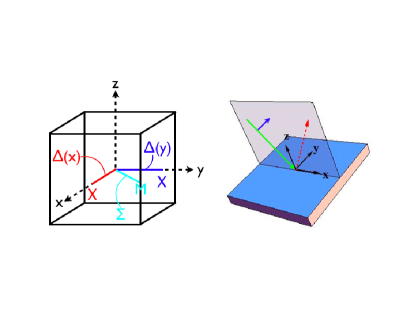
Figure 1: (Color online) Left: High symmetry points and lines in the Brillouin Zone (BZ) of a simple cubic lattice. Right: Experimental geometry used in simulations of ARPES data in the [10] BZ. The photon source (green), with polarization in the xz-plane (blue), excites an electron to a high energy state that is emitted towards the detector (red dashed). Although the experimental geometry is unchanged by a reflection through the xz-plane, the yz and xy orbitals are odd under this operation. This leads to measurement of only the zx band in this measurement.

We illustrate the usefulness of the matrix element effect by considering $M$ for $\bm{G}=\bm{0}$ ([00] BZ) and for $\bm{G}$ along the $x$-axis ([10] BZ). In the first case $M$ always vanishes since all $\xi_{j}$’s are odd with respect to reflection off either the z-x or the z-y plane. There is therefore no ARPES signal in the [00] BZ for $t_{2g}$ conduction band states. For the [10] BZ

$$M^{[01]}\propto\int\bm{dr}dze^{-i\left(G_{x}x+p_{z}z\right)}Y(\bm{r},z).$$ (22)

Contributions from other $t_{2g}$ components of $\Psi_{i}$ vanish because of their reflection symmetry in the x-z mirror plane (see Fig.1). Therefore only wave functions containing a $Y$ orbital will be detected in this case. Recent experimentsChang ; Meevasana on bulk SrTiO₃ find a single (doubly degenerate) band for $k_{z}=0$ in the [01] BZ in the cubic as well as in the tetragonal phase (see section IV). The Hamiltonian described by Eqs.(6—10) then indicates that the ${\cal N}$’s and $\Delta_{\mbox{\tiny SO}}$ must be sufficiently small so that any hybridization between the $t_{2g}$-orbitals is negligible. (see Fig.2).

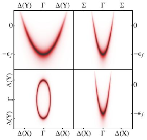
Figure 2: (Color online) Simulated ARPES signal in the [10] BZ for a temperature of $120K$, $L/M=1/8$, $\Delta_{\mbox{\tiny SO}}=0$, and $N=0$. The resolution for all ARPES simulations was set to $10$meV. Only a single elliptical FS cross-section is seen (bottom left). Energy distribution curves (EDCs) have been included along several high symmetry directions - in this case showing only a single band associated with the $xz$ basis state.

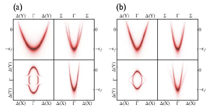
Figure 3: (Color online) Comparison of d-orbital mixing. Simulated ARPES signal for a temperature of $120K$, $L/M=1/8$, and $\Delta_{\mbox{\tiny T}}=0$. (a) For $N/M=3$ and $\Delta_{\mbox{\tiny SO}}=0$ the hybridization is most pronounced along $\Sigma$ but unseen in the EDCs along $\Delta(X)$, and $\Delta(Y)$. (b) For $N/M=0$ and $\Delta_{\mbox{\tiny SO}}=3\epsilon_{F}$ one band has moved above the Fermi energy. The hybridization between the basis states is seen in the EDCs along all directions. This experimental feature can be attributed to the lack of a preferential direction of the SO interaction.

As evident from the Hamiltonian (3) and illustrated in Fig.3 the $t_{2g}$ d-orbitals are hybridized by $N$. The influence of $N$ is most pronounced along the main diagonals. For example in the $[110]$ direction $N$ induces a momentum dependent gap of $2Nk^{2}$.

Spin-orbit interactions will also mix the $t_{2g}$ d-orbitals however in contrast to the $N\neq 0$ scenario they have no preferential direction. When the SO splitting is larger than the Fermi energy, the ARPES spectrum along the $\Sigma$ direction is similar to the spectrum in the $N\neq 0$, $\Delta_{\mbox{\tiny SO}}=0$ case. However, unlike the $N\neq 0$ case the photoemission spectrum is also altered along the $\hat{\bm{x}}$ and $\hat{\bm{y}}$ directions. This is evident along $k_{x}$ in the simulated ARPES data of Fig.3, where the induced hybridization of the basis functions cause the previously dark band to become visible.

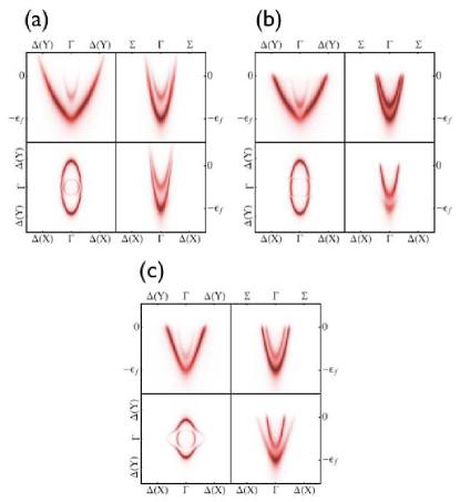
Figure 4: (Color online) Simulated ARPES measurement for the [10] BZ for different values of $\Delta_{\mbox{\tiny SO}}$ and $\Delta_{\mbox{\tiny T}}$. $L/M=1/8$, and $N=0$ in all figures. (a) $T=120K$, $\Delta_{\mbox{\tiny SO}}=0.5\epsilon_{\mbox{\tiny F}}$, $\Delta_{\mbox{\tiny T}}=0$. As evident from all EDCs the SO splitting hybridizes the basis states. If the temperature is lowered, inducing a structural phase transition that is large, one band moves above the Fermi energy. This relatively weak hybridization is seen in the Fermi surface (FS) of (b) where $T=20K$, $\Delta_{\mbox{\tiny SO}}=0.5\epsilon_{\mbox{\tiny F}}$, $\Delta_{\mbox{\tiny T}}=3\epsilon_{\mbox{\tiny F}}$. In contrast, for $T=20K$, $\Delta_{\mbox{\tiny SO}}=3\epsilon_{\mbox{\tiny F}}$, $\Delta_{\mbox{\tiny T}}=0.5\epsilon_{\mbox{\tiny F}}$ the strong hybridization of the basis states leads to a more symmetric FS (c). This feature is also seen by comparing the EDCs of (b) and (c).

The SO and tetragonal energies $\Delta_{\mbox{\tiny SO}}$ and $\Delta_{\mbox{\tiny T}}$ determine the band splitting at the $\Gamma$ point (see Eq.(LABEL:E_tetragonal)). In the cubic phase the value of $\Delta_{\mbox{\tiny SO}}$ can be extracted directly from an ARPES measurement in the $[10]$ surface BZ (see Fig. 4a). This simple picture is complicated in the tetragonal phase. The case where $\Delta_{\mbox{\tiny SO}}>\epsilon_{\mbox{\tiny F}}$ and $\Delta_{\mbox{\tiny T}}<\epsilon_{\mbox{\tiny F}}$ is readily distinguished from the opposite limit by analysis of the dispersion along $k_{x}$. As evident from Figs. 4b and 4c only in the case where $\Delta_{\mbox{\tiny SO}}>\epsilon_{F}$, is the dark weakly dispersive band visible away from the $\Gamma$ point. When both $\Delta_{\mbox{\tiny SO}}$ and $\Delta_{\mbox{\tiny T}}$ are less than the Fermi energy, the Energy Distribution Curves (EDCs) at the $\Gamma$ point can be used to distinguish between the two cases. This can be seen in Fig. 5.

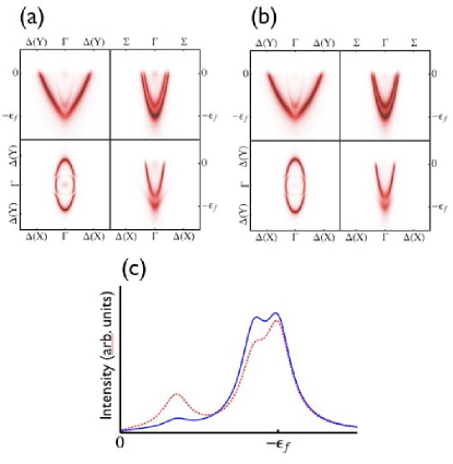
Figure 5: (Color online) When $\Delta_{\mbox{\tiny SO}}$ and $\Delta_{\mbox{\tiny T}}$ are both small, although all three bands can be seen directly in a measurement of the $[10]$ BZ it can be unclear how to extract these parameters. This is seen by comparing (a) where $\Delta_{\mbox{\tiny SO}}=.5\epsilon_{\mbox{\tiny F}}$. $\Delta_{\mbox{\tiny T}}=0.3\epsilon_{\mbox{\tiny F}}$ with (b) where $\Delta_{\mbox{\tiny SO}}=0.3\epsilon_{\mbox{\tiny F}}$. $\Delta_{\mbox{\tiny T}}=0.5\epsilon_{\mbox{\tiny F}}$. A careful analysis of the EDC at the $\Gamma$ point can distinguish between the two scenarios. This is shown in (c) where the $\Gamma$ point EDC is shown for (a) in dashed-red and for (b) in blue.

III.3 Magnetic Oscillations

Magnetic oscillations in various physical properties such as the conductivity (Shubnikov - de Haas effect) and the magnetic susceptibility (de Haas - van Alfen effect) provide invaluable information on the band structure of solidsAshcroft ; Marder ; Kubler ; Singleton . The frequency of the oscillations $F$ is related to the extremal cross-sectional area $A_{k}$ of the Fermi surface in a plane perpendicular to the magnetic field through the Onsager relation $F=\phi_{0}A_{k}/4\pi^{2}$. Here $\phi_{0}=hc/e$ is the magnetic flux quantum. Measuring $F$ as a function of charge density, magnetic field orientation, and temperature also makes it possible in principle to determine all the phenomenological Hamiltonian parameters.

In the naive picture of three ellipsoidal decoupled d-bands the cross sectional areas are simply given by ellipses. However this oversimplified scenario breaks down for any realistic system due to the hybridization of the d-orbitals by $N$, and by the SO interactions. Avoided crossings of the overlapping energy bands then result in more complicated energy surfaces.

To illustrate the variety of possible shapes of electron pockets we consider a simple case with a small but finite band mixing (e.g. $N\gtrsim 0$). $\Delta_{\mbox{\tiny T}}/\epsilon_{\mbox{\tiny F}}=0.5$.

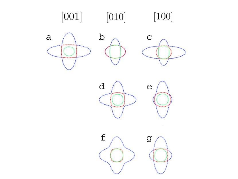
Figure 6: (Color online) Extremal cross sectional areas for magnetic field oriented along [001] (left) [010] (center) and [100] (right). The extremal orbits have been organized by size from largest to smallest and shown as dashed-blue, dot-dashed-red, and dotted-green, respectively. Top row (a-c) corresponds to $\Delta_{\mbox{\tiny T}}=0.5\epsilon_{\mbox{\tiny F}}$, middle row (d,e) corresponds to $\Delta_{\mbox{\tiny SO}}=0.5\epsilon_{\mbox{\tiny F}}$, and bottom row corresponds to $N=0.5M$.

The cross sectional areas for three high symmetry directions of the magnetic field are depicted in the top row of Fig.6 for the tetragonal phase. As $\Delta_{\mbox{\tiny T}}$ increases the most energetic band is gradually depleted and the electronic charge is redistributed amongst the other two Fermi pockets. Eventually for $\Delta_{\mbox{\tiny T}}/\epsilon_{\mbox{\tiny F}}>1-\textrm{min}(L/M,M/L)$ there is no band crossing between the $xy$-band and the other two bands.

Avoided crossings in the cubic phase result in non-elliptical cross-sections as well. The extremal cross-sectional areas along high symmetry directions are depicted in Fig.6 for $\Delta_{\mbox{\tiny SO}}/\epsilon_{\mbox{\tiny F}}=0.5$ (center row) and for $N/M=0.5$ (bottom row).

Our discussion ignores the possibility of multiple domains in the distorted state, and neglects magnetic breakdown. The latter is likely present in magnetic oscillation measurements on these materials because of the close approaches between extremal cross-sections Chambers belonging to different bands.

IV $\textrm{SrTiO}_{3}$

Bulk STO is a band insulator with an energy gap of $3.2$ eV. By chemical substitution of the $Ti$ or the $Sr$ atoms or by introducing oxygen vacancies it is possible to electron dope the system with a high level of precision. STO has cubic symmetry at room temperature, however at 105K it undergoes a antiferrodistortive structural transition to a tetragonal phase. Below the critical temperature neighboring $TiO_{6}$ octahedras continuously rotate in opposite directions by an angle of up to a few degrees.

Although STO has been studied for many years, there are only a few experimental results that can shed light on the structure of its conduction bands. We therefore resort to a 5-parameter model in which the Hamiltonian is parameterized by $\Delta_{\mbox{\tiny SO}},\Delta_{\mbox{\tiny T}},M,N$, and $L$, i.e. $h$ is approximated by its cubic phase form.

The experiments that do exist appear to partially contradict one another. Based on Raman spectroscopy and Shubnikov de-Hass measurements Uwe et. al.UweRaman ; UweSdH concluded that $\Delta_{\mbox{\tiny SO}}\approx 18$meV and $\Delta_{\mbox{\tiny T}}\approx 1.5$meV. On the contrary, Chang et. al.Chang using ARPES do not observe a SO induced gap at the zone center and conclude that $\Delta_{\mbox{\tiny T}}\approx-25$meV.

Supporting evidence for the smallness of $\Delta_{\mbox{\tiny SO}}$ is provided by the matrix element effect. ExperimentsChang observe only, what should be according to our matrix element analysis, the X orbital in the [10] BZ and the Y orbital in the [01] BZ. As explained in section III.2, the lack of hybridization between $t_{2g}$ orbitals implies that both $\Delta_{\mbox{\tiny SO}}$ and $N$ are very small. Additional proof that $N\ll M,L$ is provided the ARPES EDCs which reveal no special features of the energy along $\Sigma$. In addition, these curves yield values for the effective masses from which it follows that

$$M\approx 0.84\ ,\ L\approx 0.14.$$ (23)

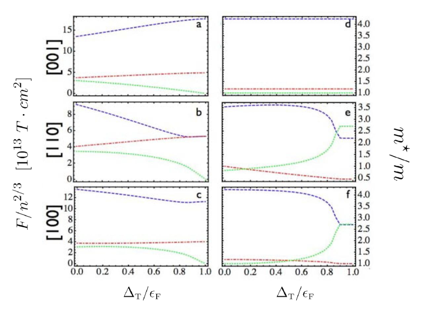
Figure 7: (Color online) Dependence of magnetic oscillation frequency and cyclotron mass on $\Delta_{\mbox{\tiny T}}$. Here we set $L/M=1/8$, $N=0$, and $\Delta_{\mbox{\tiny SO}}=0$. (a,b,c): Scaled SdH frequency for magnetic fields along $[001]$, $[110]$, and $[100]$ as a function of $\Delta_{t}$. (d,e,f): Cyclotron mass as a function of $\Delta_{\mbox{\tiny T}}$.

Raman spectroscopy measurementsUweRaman find energy gaps of approximately 2meV and 18 meV between conduction bands at the $\Gamma$ point suggesting that $\Delta_{\mbox{\tiny T}}$ and $\Delta_{\mbox{\tiny SO}}$ have very different magnitudes. The larger of the two scales can be identified as tetragonal or spin-orbit from the dependence of magnetic oscillation frequency $F$ and cyclotron mass $m^{\star}$ on density and field orientation. Fig.7 depicts the dependence of $F$ and $m^{\star}$ on density and on $\Delta_{\mbox{\tiny T}}$. The dependence can be expressed through a single parameter $\Delta_{\mbox{\tiny T}}/\epsilon_{\mbox{\tiny F}}$ if $F$ is scaled with $n^{2/3}$ where $n$ is the electronic density. Similar graphs are given in Fig.8 for a scenario in which $\Delta_{\mbox{\tiny T}}\ll\Delta_{\mbox{\tiny SO}}$. The different trends of $F$ and $m^{\star}$ as a function of density clearly distinguishes between the $\Delta_{\mbox{\tiny T}}\gg\Delta_{\mbox{\tiny SO}}$ scenario and its opposite counterpart.

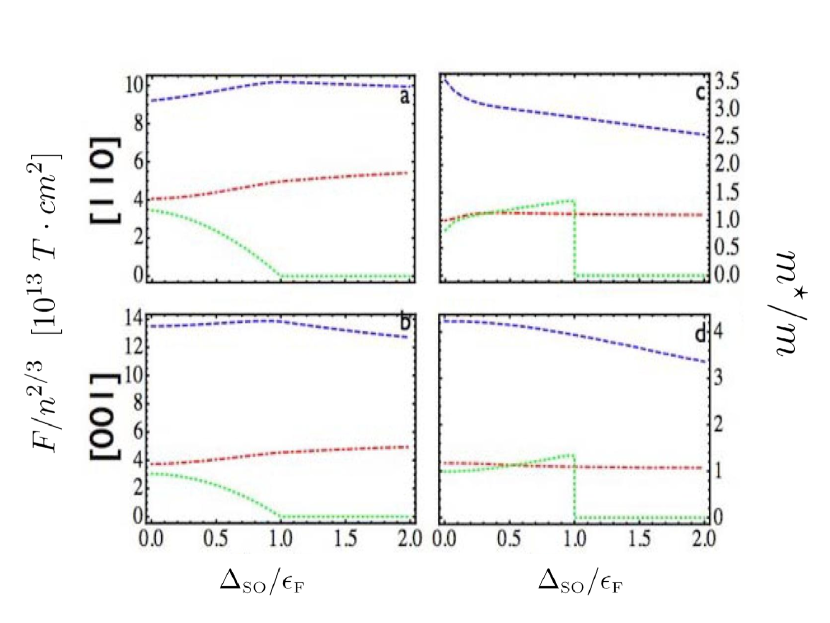
Figure 8: (Color online) Dependence of magnetic oscillation frequency and cyclotron mass on $\Delta_{\mbox{\tiny SO}}$. Here $L/M=1/8$, $N=0$ and $\Delta_{\mbox{\tiny T}}=0$. (a,b): Scaled SdH frequency for magnetic fields along $[001]$, $[110]$, and $[100]$ as a function of $\Delta_{\mbox{\tiny SO}}$. (c,d): Cyclotron mass as a function of $\Delta_{\mbox{\tiny SO}}$.

V Summary

$d^{0}$ Perovskites have played a centeral role in various areas of solid state physics and are now emerging as important building blocks for oxide-based hetro-structures. In this work we used the $\bm{k\cdot p}$ theory to construct the general low energy theory for the conduction bands of these materials both in the cubic and in the tetragonal phases. We then employed the theory to estimate the Hamiltonian parameters for STO.

Our work emphasizes the need for additional experimental data on the electronic band structure of Perovskites. Even for STO, by far the most studied $d^{0}$ Perovskite, existing experimental data is insufficient to uniquely determine the values of band parameters that will, for example, control the character of the two-dimensional electron systems formed by $\delta$-doping.

In the past few years much effort has been devoted to fabricating oxide-based hetro-structures. Our model for the electronic structure of the bulk is a first step towards modeling these complex systems.

This work was supported by Welch Foundation Grant F1473. We acknowledge helpful conversations with Jim Allen, Young Jun Chang, Harold Hwang, Worawat Meevasana, and Susanne Stemmer.

Appendix A $\bm{k\cdot p}$ Hamiltonian for the tetragonal phase

The momentum dependent part of the effective hamiltonian $h$ for a $d^{0}$ perovskite is given by Eq.(3). In this appendix we use group theory methods to express $h$ in terms of a small number of phenomenological parametersDresselhaus .

The calculation of $h$ involves the evaluation of matrix elements of the form $\langle\phi|\bm{k\cdot p}|\psi_{j}\rangle$. Here $\psi_{j}$ is a basis function of the $t_{2g}$ manifold, $\bm{p}$ is the momentum operator, and $\phi$ is a state outside of the $t_{2g}$ manifold. At the cubic to tetragonal phase transition the symmetry at the zone center reduces from $O_{h}$ to $D_{4h}$. Correspondingly, at the phase transition the three $\psi_{j}$’s change their transformation properties $\Gamma_{25}^{+}\to\Gamma_{4}^{+}+\Gamma_{5}^{+}$. The three components of the momentum operator $\bm{p}$, that transform as a single irrep ($\Gamma_{15}^{-}$) in the cubic phase split: $p_{x},p_{y}\in\Gamma_{5}^{-}$ whereas $p_{z}\in\Gamma_{2}^{-}$.

The values of the matrix elements vary smoothly across the structural transition. To emphasize the relation between the two symmetries we label the matrix elements in the tetragonal phase with a subscript that corresponds to the irrep of $\phi$ in the cubic phase and a superscript that corresponds to its irrep in the tetragonal phase . For example, $B^{5}_{15}$ is associated with a basis function that evolved from $\Gamma_{15}$ in the cubic phase to $\Gamma_{5}$ in the tetragonal one.

We first consider the $\Gamma_{4}^{+}$ band. The intermediate states are

$$\Gamma_{5}^{-}\otimes\Gamma_{4}^{+} = \Gamma_{5}^{-}$$

$$\Gamma_{2}^{-}\otimes\Gamma_{4}^{+} = \Gamma_{3}^{-}.$$ (24)

Denoting

$$\langle\Gamma_{5x}^{-}|(p_{x},p_{y})|\Gamma_{4}^{+}\rangle = \left\{\begin{array}[]{c}B_{15}^{5}(0,1)\\ B_{25}^{5}(0,1)\end{array}\right.$$ (27)

$$\langle\Gamma_{5y}^{-}|(p_{x},p_{y})|\Gamma_{4}^{+}\rangle = \left\{\begin{array}[]{c}B_{15}^{5}(1,0)\\ -B_{25}^{5}(1,0)\end{array}\right.$$ (30)

$$\langle\Gamma_{3}^{-}|p_{z}|\Gamma_{4}^{+}\rangle = \left\{\begin{array}[]{c}B_{2}^{3}\\ B_{12}^{3}\end{array}\right.,$$ (33)

we find that

$$h_{zz}={\cal M}_{B}(k_{x}^{2}+k_{y}^{2})+{\cal L}_{B}k_{z}^{2}$$ (34)

where the two real phenomenological parameters are given by

$${\cal M}_{B}=\frac{1}{2m}+\frac{1}{m^{2}}\sum_{n^{\prime}\in\Gamma_{5}^{-}}\frac{|B_{n^{\prime}}^{5}|^{2}}{E^{\Gamma_{4}^{+}}(0)-E_{n^{\prime}}^{\Gamma_{5}^{-}}(0)},$$ (35)

and

$${\cal L}_{B}=\frac{1}{2m}+\frac{1}{m^{2}}\sum_{n^{\prime}\in\Gamma_{3}^{-}}\frac{|B_{n^{\prime}}^{3}|^{2}}{E^{\Gamma_{4}^{+}}(0)-E_{n^{\prime}}^{\Gamma_{3}^{-}}(0)}.$$ (36)

We now turn to the $\Gamma_{5}^{+}$ band. The intermediate states are

$$\Gamma_{5}^{-}\otimes\Gamma_{5}^{+} = \Gamma_{1}^{-}+\Gamma_{2}^{-}+\Gamma_{3}^{-}+\Gamma_{4}^{-}$$

$$\Gamma_{2}^{-}\otimes\Gamma_{5}^{+} = \Gamma_{5}^{-}.$$ (37)

Following similar steps to those taken above we obtain expression (10). The k-dependent Hamiltonian $h$ depends on six real parameters and a single complex parameter ${\cal N}_{BC}$. The $\bm{k\cdot p}$ Hamiltonian in the cubic phase can easily be obtained from its tetragonal counterpart by disregarding the subscripts of the phenomenological parameters; for example by associating with ${\cal L}_{B}$ and ${\cal L}_{C}$ a single parameter ${\cal L}$.

References

- (1) S. Jin, T. H. Tiefel, M. McCormack, R. A. Fastnacht, R. Ramesh, L. H. Chen, Science , 413 (1994).
- (2) J. G. Bednroz K. A. Muller, Z. Phys. B , 189 (1986).
- (3) K. Rabe, Ch. H. Ahn J.-M. Triscone, Physics of Ferroelectrics, (Springer 2007).
- (4) J. B. Goodenough, Localized to intinerant ekectronic transition in perovskite oxides (Springer 1996)
- (5) J. Son et. al. Nature Mat. 10.1038/nmat2750 (2010)
- (6) H. Nakamura and T. Kimura, Phys. Rev. B 80, 121308(R) (2009).
- (7) A. Ohtomo, H. Y. Hwang, Nature , 423 (2004).
- (8) A. Brinkman et. al., Nature Mat. , 493 (2007).
- (9) M. Ben Shalom, Phys. Rev. B , 140403 (2009)
- (10) S. Seri, L. Klein, Phys. Rev. B 80, 180410(R) (2009).
- (11) Y. Kozuka et. al., Nature , 487 (2009).
- (12) J. Mannhart et. al., MRS Bulletin , 1027 (2008).
- (13) J. Heber, Nature , 28 (2009).
- (14) L. F. Mattheiss, Phys. Rev. B 6, 4718 (1972).
- (15) L. F. Mattheiss, Phys. Rev. B 6, 4740 (1972).
- (16) T. Neumann, G. Borstel, C. Scharfschwerdt, M. Neumann, Phys. Rev. B 46, 10623 (1992).
- (17) M. S. Dresselhaus, G. Dresselhaus, A. Joiro, Group Theory (Springer, 2008).
- (18) Y. Yu, M. Cardona, Fundamentals of Semiconductors (Springer, 1996).
- (19) L. Cao, E. Sozontov, J. Zegnhagen, Phys. Stat. Sol. (a) , 387 (2000).
- (20) A. Damascelli, Z. Hussain, and Z.-X. Shen, Rev. Mod. Phys. , 473 (2003).
- (21) J.B. Pendry, Surf. Sci.
- (22) W. Meevasana et. al., New Journal of Physics 023004 (2010).
- (23) Y. J. Chang et. al., arXiv:1002.0962
- (24) H. Uwe, et. al., Jap. J. Appl. Phys. , 335 (1985).
- (25) N. W. Ashcroft, N. Mermin, Solid State Physics (Thomson Learning Inc., 1976).
- (26) M. P. Marder, Condensed Matter Physics (John Wiley & Sons, Inc. 2000).
- (27) J. Kubler, Theory of Itinerant Electron Magnetism (Oxford University Press Inc., 2000).
- (28) J. Singleton , Band theory and electronic properties of soilds (Oxford University Press Inc., 2001).
- (29) R. G. Chambers, Proc. Phys. Soc. , 701 (1966).
- (30) H. Uwe, T. Sakudo, H. Yamaguchi, Jap. J. Appl. Phys. , 519 (1985).