On the Rate Achievable for Gaussian Relay Channels Using Superposition Forwarding

Abstract

We analyze the achievable rate of the superposition of block Markov encoding (decode-and-forward) and side information encoding (compress-and-forward) for the three-node Gaussian relay channel. It is generally believed that the superposition can out perform decode-and-forward or compress-and-forward due to its generality. We prove that within the class of Gaussian distributions, this is not the case: the superposition scheme only achieves a rate that is equal to the maximum of the rates achieved by decode-and-forward or compress-and-forward individually. We also present a superposition scheme that combines broadcast with decode-and-forward, which even though does not achieve a higher rate than decode-and-forward, provides us the insight to the main result mentioned above.

I Introduction

The relay channel, introduced by van der Meulen [1] is a fundamental building block in network information theory. It consists of a relay terminal assisting communication between a source terminal and a destination terminal, facilitating a higher data rate than that of a point to point channel. Cover and El Gamal [2] introduced two new coding strategies and a cut-set upper bound for the relay channel. They derived the capacity of the degraded and reversely degraded relay channels. Capacity results have been derived for special cases of the relay channel like the semi-deterministic case [3] but the capacity of the general relay channel is still unknown.

The main achievability strategies known for the relay channel are Decode and Forward (DF) and Compress and Forward (CF) [2]. The DF scheme is also known as the general block Markov encoding scheme. The relay decodes the transmitted message and jointly transmits the message from the source to the destination terminal. The DF strategy is optimal and achieves the cut-set bound when the source to relay link channel is strong. The CF scheme is known as the side-information encoding scheme. The relay compresses the received signal without decoding and transmits to the destination terminal. The destination terminal treats the compressed information as side information and decodes the original message. The CF scheme is asymptotically optimum and achieves the cut-set bound when the relay to destination link channel is strong, so that the received signal at the relay can be conveyed faithfully to the destination. A combination of the two strategies that superimposes DF and CF was also proposed in [2, Theorem 7]. Hereafter we refer to this scheme as the superposition forwarding (SF). The SF scheme achieves the capacity for the special cases of degraded, reversely degraded and semi-deterministic relay channels. Due to the generality of the result in [2, Theorem 7], it is expected it can offer higher achievable rates than DF or CF alone.

In this paper, we investigate the coding scheme for the general Gaussian relay channel. The initial motivation for the work was to develop new coding strategies with higher achievable rates. A new coding strategy was designed which superimposes Decode and Forward and Broadcast, as presented in Section III. The scheme unfortunately yields a rate that is inferior to DF. This attempt, though not successful, prompted us to investigate the general superiority of SF, especially for the Gaussian relay channel. It is found that for Gaussian relay channel, within the class of Gaussian distributions, the SF can achieve at most the larger rate achievable by DF or CF alone — there is no need to do superposition for Gaussian distributions (Section IV). We also provide one numerical example that verified the theoretical result in Section V. Section VI concludes the paper.

Notation: For random variables $X,Y,Z$, we use $p(x,y,z)$ to denote the joint distribution, when there is no confusion, as a short cut to $p_{X,Y,Z}(x,y,z)$. When $X$ and $Z$ are conditionally independent given $Y$ (i.e., $X,Y$, and $Z$ form a Markov chain), we write $X-Y-Z$.

II Preliminaries

We present the mathematical models for the discrete-memoryless and Gaussian relay channels in this section, and also include the known results on achievable rates that will be used later.

II-A Discrete memoryless relay channel

The general discrete memoryless relay channel (DMRC) is the same as defined in [2]. A brief description is given here for completeness. The DMRC is denoted by $({\mathcal{X}}_{1}\times{\mathcal{X}}_{2},p(y_{2},y_{3}|x_{1},x_{2})$, ${\mathcal{Y}}_{2}\times{\mathcal{Y}}_{3})$, where ${\mathcal{X}}_{1},{\mathcal{X}}_{2},{\mathcal{Y}}_{2},{\mathcal{Y}}_{3}$ are finite sets and $p(.,.|x_{1},x_{2})$ is a collection of probability distributions on ${\mathcal{Y}}_{2}\times{\mathcal{Y}}_{3}$, one for each $(x_{1},x_{2})\in{\mathcal{X}}_{1}\times{\mathcal{X}}_{2}$; $x_{1}$ and $x_{2}$ are the transmitted symbols at the source and the relay respectively; $y_{2}$ and $y_{3}$ are the received symbols at the relay and the destination terminal.

An $(M,n)$ code for the relay channel consists of a set of integers ${\mathcal{M}}=\{1,2,\ldots,M\}$, an encoding function $x_{1}:{\mathcal{M}}\rightarrow{\mathcal{X}}_{1}^{n}$ a set of relay functions $\{f_{i}\}_{i=1}^{n}$ such that

$$x_{2i}=f_{i}\left(Y_{21},Y_{22},\ldots,Y(2i-1)\right),\hskip 10.0pt1\leq i\leq n,$$

and a decoding function $g:{\mathcal{Y}}_{3}^{n}\rightarrow{\mathcal{M}}$. The joint probability mass function on ${\mathcal{M}}\times{\mathcal{X}}_{1}^{n}\times{\mathcal{X}}_{2}^{n}\times{\mathcal{Y}}_{2}^{n}\times{\mathcal{Y}}_{3}^{n}$ is

$$p(w,x_{1},x_{2},y_{2},y_{3})=p(w)\prod_{i=1}^{n}p(x_{1i}|w)p(x_{2i}|y_{21},y_{22},\ldots,y_{2i-1})p(y_{2i},y_{3i}|x_{1i},x_{2i}).$$ (1)

Define $\lambda(w)=p(g(Y)\neq w)$ as the probability of error of the decoding function of the relay channel and let $\lambda_{n}$ be the maximal probability of error over all possible messages $w$. The rate $R=(1/n)\log M$ of an $(M,n)$ code is said to be achievable by a relay channel if for any $\epsilon>0$ and for sufficiently large $n$, there exists a code with $M\geq 2^{nR}$ such that $\lambda_{n}<\epsilon$.

II-B Gaussian relay channel

Fig. 1 shows the Gaussian relay channel model that we will be using. The received symbols at the relay and the destination terminal are given respectively by

$$Y_{2} = aX_{1}+Z_{1}$$ (2)

$$Y_{3} = X_{1}+bX_{2}+Z_{2}$$ (3)

where the noise terms $Z_{1}$ and $Z_{2}$ are uncorrelated zero mean Gaussian random variables with variances $N_{1}$ and $N_{2}$ respectively, and $a$ and $b$ are the channel gain constants. As a result, we have

$$p(y_{2},y_{3}|x_{1},x_{2})=\frac{1}{2\pi\sqrt{N_{1}N_{2}}}\exp\left[-\frac{(y_{2}-ax_{1})^{2}}{2N_{1}}-\frac{(y_{3}-x_{1}-bx_{2})^{2}}{2N_{2}}\right],$$ (4)

which will be the channel assumed throughout the paper.

The average power constraints at the transmitters are

$$\frac{1}{n}\sum_{i=1}^{n}x_{1i}^{2}(k) \leq P_{1},\quad\forall k\in{\mathcal{M}},$$ (5)

and

$$\frac{1}{n}\sum_{i=1}^{n}x_{2i}^{2} \leq P_{2},\quad\forall y_{2}^{n}\in\Re^{n}.$$ (6)

II-C Known achievable rates

We briefly review the known results in for DF, CF, and the SF. For DMRC, the DF scheme achieves any rate less than [2, Theorem 1]

$$R_{DF}=\sup\min\{I(X_{1};Y_{2}|X_{2}),I(X_{1},X_{2};Y_{3})\}$$ (7)

where the supremum is taken over all possible $p(x_{1},x_{2})$. The CF scheme achieves any rate less than [2, Theorem 6]

$$R_{CF}=\sup I(X_{1};\hat{Y}_{2},Y_{3}|X_{2}),\quad\text{such that }I(X_{2};Y_{3})\geq I(\hat{Y}_{2};Y_{2}|X_{2},Y_{3})$$ (8)

where supremum is taken over all joint probability distributions of the form

$$p(x_{1},x_{2},y_{2},y_{3},\hat{y_{2}})=p(x_{1})p(x_{2})p(y_{2},y_{3}|x_{1},x_{2})p(\hat{y}_{2}|y_{1},x_{2}).$$ (9)

El Gamal, Mohseni, and Zahedi [4] put forth an equivalent characterization of the CF scheme. That is, it achieves any rate less than

$$R_{CF}=\sup\min\{I(X_{1};\hat{Y}_{2},Y_{3}|X_{2}),I(X_{1},X_{2};Y_{3})-I(\hat{Y}_{2};Y_{2}|X_{1},X_{2},Y_{3})\}\\$$ (10)

where supremum is still taken over all joint probability distributions of the same form as in (9). The supremum of rates achievable by superimposing DF and CF [2, Theorem 7] is

$$R_{SF}=\sup(\min\{I(X_{1};Y_{3},\hat{Y}_{2}^{\prime}|X_{2},U)+I(U;Y_{2}|X_{2},V),\\ \quad I(X_{1},X_{2};Y_{3})-I(\hat{Y}_{2}^{\prime};Y_{2}|U,X_{1},X_{2},Y_{3})\})$$ (11)

where the supremum is over all joint probability distributions of the form

$$p(u,v,x_{1},x_{2},y_{2}^{\prime},y_{3},\hat{y_{2}})=p(v)p(u|v)p(x_{1}|u)p(x_{2}|v)p(y_{2},y_{3}|x_{1},x_{2})p(\hat{y}_{2}^{\prime}|x_{2},y_{2},u)$$ (12)

subject to the constraint

$$I(X_{2};Y_{3}|V)\geq I(\hat{Y}^{\prime}_{2};Y_{2}|X_{2},Y_{3},U).$$ (13)

Finally, the rate is upper bounded by the cut-set bound

$$R_{CS}=\sup\min\{I(X_{1},X_{2};Y_{3}),I(X_{1};Y_{2},Y_{3})\},$$ (14)

where the supremum is taken over all possible distributions $p(x_{1},x_{2})$.

III Broadcast over Decode and Forward

Before investigating the coding scheme that superimposes CF and DF for the Gaussian relay channel, we will first look at a simpler coding scheme. In this scheme, partial information is decoded first at both the relay and the destination terminals like in a broadcast channel. The remaining message is decoded and forwarded given the partial information available at the relay and destination terminal. The coding scheme is equivalent to superimposing broadcast over decode and forward.

We split the message $W$ into two parts $W^{\prime}$ and $W^{\prime\prime}$ with respective rates $R^{\prime}$ and $R^{\prime\prime}$. We demand $W^{\prime}$ be decoded at both relay and destination. The relay also decodes the message $W^{\prime\prime}$ which the destination could not decode and sends this extra information to the destination in a block Markov encoding fashion. This strategy can be designed using an auxiliary random variable $U$ and a block Markov superposition encoding explained below.

Theorem 1

For any relay channel (${\mathcal{X}}_{1}\times{\mathcal{X}}_{2},p(y_{2},y_{3}|x_{1},x_{2}),{\mathcal{Y}}_{2}\times{\mathcal{Y}}_{3}$), the rate $R$ is achievable where

$$R<\sup_{P}\{\min\{I(U;Y_{3}),I(U;Y_{2}|X_{2})\}+\min\{I(X_{1};Y_{2}|X_{2},U),I(X_{1},X_{2};Y_{3}|U)\}\}$$ (15)

and the supremum is taken over all probability distribution functions of the form

$$p(u,x_{1},x_{2},y_{2},y_{3})=p(u)p(x_{2})p(x_{1}|x_{2},u)p(y_{2},y_{3}|x_{1},x_{2}).$$

Proof:

Codebook Generation

Encoding is performed in $K+1$ blocks. For each block $k$, generate $2^{nR^{\prime}}$ codewords $u_{k}^{n}(s),s=1,2,\ldots,2^{nR^{\prime}}$ by choosing the $u_{ki}(s)$ independently using the distribution $P_{U}(\cdot)$. Generate $2^{nR^{\prime\prime}}$ codewords $x_{2k}^{n}(t),t=1,2,\ldots,2^{nR^{\prime\prime}}$ by choosing $x_{2ki}(t)$ independently using the probability distribution $P_{X_{2}}(\cdot)$. Now use superposition coding and generate $2^{nR^{\prime\prime}}$ codewords $x_{1k}^{n}(r|s,t)$, $r=1,2,\ldots,2^{nR^{\prime\prime}}$ for every pair of $(u_{k}^{n}(s),x^{n}_{2k}(t))$, by choosing the $x_{1k,i}(r|s,t)$ independently using $P_{(X_{1}|X_{2},U)}(.|u_{k,i}(s),x_{2k,i}(t))$.

Encoding

Let $s_{k}$ be the message index of $W^{\prime}$ and $t_{k}$ be the message index of $W^{\prime\prime}$ respectively to be sent in block $k$. The source encoder then transmits $x_{1k}^{n}(t_{k}|s_{k},t_{k-1})$ where $t_{k-1}$ is the index of $W^{\prime\prime}$ sent in the previous block. The relay in block $k$ will send $x_{2k}^{n}(\hat{t}_{k-1})$, where $\hat{t}_{k-1}$ is the estimate of $t_{k-1}$ at the relay.

Decoding at relay terminal

Assume that decoding of $s_{k-1}$ and $t_{k-1}$ in block $k-1$ has been successful. Upon receiving $y_{2k}^{n}$ in block $k$, the relay looks for a unique $\hat{s}_{k}$ such that

$$\left(u_{1k}^{n}(\hat{s}_{k}),x_{2k}^{n}(\hat{t}_{k-1}),y_{2k}^{n}\right)\in T_{\epsilon}^{n}(P_{U,X_{2},Y_{2}}).$$

Having decoded $\hat{s}_{k}$, the relay now looks for a unique $\hat{t}_{k}$ such that

$$\left(x_{1k}^{n}(\hat{t}_{k}|\hat{s}_{k},\hat{t}_{k-1}),u_{1k}^{n}(\hat{s}_{k}),x_{2k}^{n}(\hat{t}_{k-1}),y_{2k}^{n}\right)\in T_{\epsilon}^{n}(P_{U,X_{1},X_{2},Y_{2}}).$$

Decoding at the sink terminal

Upon receiving $y_{3k}^{n}$, the destination terminal looks for a unique $\tilde{s}_{k}$ such that $\left(u_{1k}^{n}(\tilde{s}_{k}),y_{3k}^{n}\right)\in T_{\epsilon}^{n}(P_{U,Y_{3}})$. Now, the destination decodes the additional information that the source sends in a block Markov decoding fashion. The destination terminal tries to find a unique $\tilde{t}_{k-1}$ such that $\left(x_{2k}^{n}(\tilde{t}_{k-1}),u_{1k}^{n}(\tilde{s}_{k}),y_{3k}^{n}\right)\in T_{\epsilon}^{n}(P_{U,X_{2},Y_{3}})$ and

$$\left(x_{1k}^{n}(\tilde{t}_{k-1}|\tilde{s}_{k-1},\tilde{t}_{k-2}),u_{1k}^{n}(\tilde{s}_{k-1}),x_{2k}^{n}(\tilde{t}_{k-2}),y_{3(k-1)}^{n}\right)\in T_{\epsilon}^{n}(P_{U,X_{1},X_{2},Y_{3}}).$$

Rate analysis

At the relay, since we have a single user channel from $U$ to $Y_{2}$, we will be able to decode the $U$ codewords with low probability of error if $R^{\prime}<I(U;Y_{2}|X_{2})$. We can also decode the index $t_{k}$ if

$$R^{\prime\prime}<I(X_{1};Y_{2}|U,X_{2}).$$

The destination first decodes the codeword $U$ with a low probability of error provided $R^{\prime}<I(U;Y_{3})$, and then decodes the message $t_{k}$ using successive interference cancellation on the messages from the relay and the source. The message would be decoded with low probability of error provided

$$R^{\prime\prime}<I(X_{2};Y_{3}|U)+I(X_{1};Y_{3}|X_{2},U).$$

Combining all the bounds, the desired result (15) follows. ∎

In this scheme, the source message is split into two parts. The message $W^{\prime}$ is broadcast to both relay and destination. And the other message $W^{\prime\prime}$ is decoded by relay first and then cooperatively transmitted to the destination. Unfortunately, the above achievable rate does not outperform the DF strategy, as is shown below:

$$R \leq\min\{I(U;Y_{2}|X_{2})+I(X_{1};Y_{2}|X_{2},U),I(U;Y_{3})+I(X_{1}X_{2};Y_{3}|U)\}$$ (16)

$$=\min\{I(U,X_{1};Y_{2}|X_{2}),I(X_{1},X_{2};Y_{3})\}$$ (17)

$$=\min\{I(X_{1};Y_{2}|X_{2}),I(X_{1}X_{2};Y_{3})\}.$$ (18)

where (18) follows from the Markov chains $U-X_{1}-Y_{2}$ and $U-X_{1}-Y_{3}$. But (18) is the rate achieved by the Decode and Forward strategy.

Although not providing a higher rate, the above proposed scheme of broadcast over decode and forward gives us a good insight on the superposition strategy. The cause of suboptimality arises due to the fact that the messages $W^{\prime}$ and $W^{\prime\prime}$ even though are generated from the same source, act as interference on each other. This limits the rate of decoding at the relay and destination terminals. This interference would also be present if we superimpose DF and CF. The rate achievable using the superposition strategy is investigated in the next section for the case of Gaussian relay channels.

IV Achievable Rate of the Superposition Scheme

In this section, we focus on the Gaussian relay channel. We show that when considering only jointly Gaussian distribution for all the random variables involved in (11), superposition does not offer higher rate than DF or CF alone. To be more specific, we will show that when all the random variables involved are Gaussian, then $R_{SF}\leq\max(R_{DF},R_{CF})$. Trivially, only one of two cases can be true

1. Case A: $R_{DF}\geq R_{CF}$;

2. Case B: $R_{CF}>R_{DF}$.

It is then enough to show that in Case A, $R_{SF}\leq R_{DF}$; and in Case B, $R_{SF}\leq R_{CF}$.

IV-A Gaussian distribution assumption

We assume that all random variables in (11) are zero mean and jointly Gaussian distributed. The distribution will then depend only on the variances and the cross-correlations of the random variables. For two generic random variables $X$ and $Y$, let

$$\phi_{X,Y}:=\frac{E\left\{(X-E[X])(Y-E[Y])\right\}}{\sqrt{E[X^{2}]E[Y^{2}]}}$$

denote the correlation coefficient between them. The following lemma is useful in deducing correlations from known ones.

Lemma 1

Let $X-Y-Z$ be a Markov chain of jointly Gaussian random variables. Then $\phi_{X,Z}=\phi_{X,Y}\phi_{Y,Z}$.

Proof:

See appendix. ∎

Returning to the random variables involved in $R_{SF}$, we denote $\alpha=\phi_{U,V}$, $\beta=\phi_{V,X_{2}}$, and $\gamma=\phi_{U,X_{1}}$. Using Lemma 1, we obtain from the Markov chain $U-V-X_{2}$ that

$$\delta :=\phi_{X_{1},X_{2}}=\phi_{V,U}\cdot\phi_{V,X_{2}}=\alpha\beta,$$ (19)

and from the Markov chain $$X_{1}-U-X_{2}$$ that

$$\rho :=\phi_{X_{1},X_{2}}=\phi_{X_{1},U}\cdot\phi_{U,X_{2}}=\gamma\delta=\alpha\beta\gamma.$$ (20)

Fig. 2 shows the correlation between the random variables along with their dependencies on each other.

IV-B Main Result

The main result is stated in the following theorem. Two lemmas that are needed in the proof are stated and proved in the appendix.

Theorem 2

Let $(X_{1},X_{2},Y_{2},Y_{3},\hat{Y_{2}^{\prime}},\hat{Y_{2}},U,V,)$ be a set of jointly Gaussian random variable whose joint distribution can be factorized in the following form:

$$p(u,v,x_{1},x_{2},y_{2},y_{3},\hat{y}_{2}^{\prime})=p(v)p(u|v)p(x_{2}|v)p(x_{1}|u)p(y_{2},y_{3}|x_{1}x_{2})p(\hat{y}_{2}^{\prime}|y_{2},u,x_{2})p(\hat{y}_{2}|y_{2},x_{2}),$$ (21)

where $p(y_{2},y_{3}|x_{1}x_{2})$ is as given in (4). Let ${\mathcal{P}}$ denote the class of distributions specified by (21). Let ${\mathcal{P}}^{\prime}$ denote a subset of ${\mathcal{P}}$ with distributions that also satisfy the constraint (13). We have

$$\sup_{{\mathcal{P}}^{\prime}}\min\{ I(X_{1};Y_{3},\hat{Y}_{2}^{\prime}|X_{2},U)+I(U;Y_{2}|X_{2},V),I(X_{1},X_{2};Y_{3})-I(\hat{Y}_{2}^{\prime};Y_{2}|X_{1},X_{2},U,Y_{3})\}$$ (22)

$$=\max\{ \sup_{\mathcal{P}}\min\{I(X_{1};Y_{2}|X_{2}),I(X_{1},X_{2};Y_{3})\},$$ (23)

$$\sup_{\mathcal{P}}\min\{I(X_{1};\hat{Y}_{2},Y_{3}|X_{2}),I(X_{1},X_{2};Y_{3})-I(\hat{Y}_{2};Y_{2}|X_{1},X_{2},Y_{3})\}\}.$$ (24)

Proof:

The rates appearing in (22)–(24) are $R_{SF}$, $R_{DF}$, and $R_{CF}$, respectively. Since through the judicious choice the random variables $U$ and $V$, DF and CF can be cast as special cases of SF [2], we have $R_{SF}\geq R_{DF}$ and $R_{SF}\geq R_{CF}$. It is then sufficient to show that $R_{SF}\leq\max(R_{DF},R_{CF})$.

Under the Gaussian assumption, the compressed version $\hat{Y}_{2}^{\prime}$ of $Y_{2}$ in (12) can be written as

$$\hat{Y}_{2}^{\prime}=c_{1}Y_{2}+c_{2}U+c_{3}X_{2}+Z_{w}^{\prime}$$ (25)

where $c_{1},c_{2},c_{3}$ are constant parameters, $Z_{w}^{\prime}$ is Gaussian and independent of $Y_{2}$, $U$, and $X_{2}$. Since in both (11) and (13), the three mutual information terms involving $\hat{Y}_{2}^{\prime}$, namely,

$$I(X_{1};Y_{3},\hat{Y}_{2}^{\prime}|X_{2},U),\quad I(\hat{Y}_{2}^{\prime};Y_{2}|X_{2},X_{1},U,Y_{3}),\quad I(\hat{Y}_{2}^{\prime};Y_{2}|X_{2},U,Y_{3})$$

are all conditioned on $U$ and $X_{2}$, the coefficients $c_{2}$ and $c_{3}$ do not affect the values of these terms. Therefore we can set $c_{2}=c_{3}=0$. It is also true that scaling $\hat{Y}_{2}^{\prime}$ by a constant does not change any of the terms. So unless $c_{1}=0$, we can assume $c_{1}=1$, as we do in the following. The case $c_{1}=0$ is known as the so called partial decoding and forward scheme, which is known to be inferior to the full DF scheme [4]. We denote the variance of $Z_{w}^{\prime}$ as $\Delta^{\prime}$. The amount of compression, which is controlled by the parameter $\Delta^{\prime}$, depends on the constraint (13) imposed by the relay link channel and the encoding scheme at the relay. In summary, we can take without loss of generality

$$\hat{Y}_{2}^{\prime}=Y_{2}+Z_{w}^{\prime},$$ (26)

The following is a broad outline of the proof. Given any rate achieved by the SF scheme, we can find a CF scheme or a DF scheme which can achieve a rate higher than or equal to SF. The $\hat{Y}_{2}$ for the CF scheme is set to be statistically equal to $\hat{Y}_{2}^{\prime}$ of the SF scheme in (26):

$$\hat{Y}_{2}=Y_{2}+Z_{w},$$ (27)

where $Z_{w}$ is zero mean Gaussian with variance $\Delta=\Delta^{\prime}$. Such $\hat{Y}_{2}$ would qualify as the compressed version of $Y_{2}$ in CF. This choice of $\hat{Y}_{2}$ is enough to achieve a higher rate than SF even though it can be suboptimal to the possible rates achievable by CF.

First, we have

$$I(\hat{Y}_{2}^{\prime};Y_{2}|X_{1},X_{2},U,Y_{3}) =h(Y_{2}|X_{1},X_{2},U,Y_{3})-h(Y_{2}|X_{1},X_{2},U,Y_{3},\hat{Y}_{2}^{\prime})$$ (28)

$$=h(Y_{2}|X_{1},X_{2},Y_{3})-h(Y_{2}|X_{1},X_{2},U,Y_{3},\hat{Y}_{2}^{\prime})$$ (29)

$$\geq h(Y_{2}|X_{1},X_{2},Y_{3})-h(Y_{2}|X_{1},X_{2},Y_{3},\hat{Y}_{2}^{\prime})$$ (30)

$$\geq h(Y_{2}|X_{1},X_{2},Y_{3})-h(Y_{2}|X_{1},X_{2},Y_{3},\hat{Y}_{2})$$ (31)

$$=I(\hat{Y}_{2};Y_{2}|X_{1},X_{2},Y_{3})$$ (32)

where (29) is due to the Markov chain $U-(X_{1},X_{2},Y_{3})-Y_{2}$; (30) uses the fact that conditioning does not increase entropy; and (31) is because given $(X_{2},U)$, $\hat{Y}_{2}^{\prime}$ is statistically equivalent to $\hat{Y}_{2}$.

Thus, we have shown

$$I(X_{1},X_{2};Y_{3})-I(\hat{Y}_{2}^{\prime};Y_{2}|X_{1},X_{2},U,Y_{3})\leq I(X_{1},X_{2};Y_{3})-I(\hat{Y}_{2};Y_{2}|X_{1},X_{2},Y_{3}).$$ (33)

It then remains to be shown that

$$I(X_{1};Y_{3},\hat{Y}_{2}^{\prime}|X_{2},U)+I(U;Y_{2}|X_{2},V)\leq\max\{I(X_{1};Y_{2}|X_{2}),I(X_{1};\hat{Y}_{2},Y_{3}|X_{2})\}.$$ (34)

Depending on which one of the two terms on the right hand side is bigger, we have two cases. In the first case,

$$I(X_{1};Y_{2}|X_{2})\geq I(X_{1};Y_{3},\hat{Y_{2}}|X_{2})$$ (35)

and we have

$$\quad\;\,I(U;Y_{2}|V,X_{2})+I(X_{1};Y_{3},\hat{Y_{2}^{\prime}}|X_{2},U)$$ (36)

$$=I(U;Y_{2}|V,X_{2})+I(X_{1};Y_{3},\hat{Y_{2}}|X_{2},U)$$ (37)

$$=I(U;Y_{2}|X_{2})-I(V;Y_{2}|X_{2})+I(X_{1};Y_{3},\hat{Y_{2}}|X_{2},U)$$ (38)

$$=I(X_{1};Y_{2}|X_{2})-I(X_{1};Y_{2}|X_{2},U)-I(V;Y_{2}|X_{2})+I(X_{1};Y_{3},\hat{Y_{2}}|X_{2},U)$$ (39)

$$\leq I(X_{1};Y_{2}|X_{2})-I(X_{1};\hat{Y_{2}},Y_{3}|X_{2},U)-I(V;Y_{2}|X_{2})+I(X_{1};Y_{3},\hat{Y_{2}}|X_{2},U)$$ (40)

$$=I(X_{1};Y_{2}|X_{2})-I(V;Y_{2}|X_{2})$$ (41)

$$\leq I(X_{1};Y_{2}|X_{2})$$ (42)

where (37) follows by our choice of $\hat{Y}_{2}$ to be statistically the same as $\hat{Y}_{2}^{\prime}$; (38) follows from the Markov chain $V-(U,X_{2})-Y_{2}$; (39) follows from the Markov chain $U-(X_{1},X_{2})-Y_{2}$; (40) follows from (35) and Lemma 2, which is stated and proved in Appendix -B; and (42) follows from the fact that mutual information is nonnegative.

In the second case,

$$I(X_{1};Y_{2}|X_{2})<I(X_{1};Y_{3},\hat{Y_{2}}|X_{2})$$ (43)

and we have

$$\quad\;\,I(X_{1};Y_{3},\hat{Y}_{2}^{\prime}|X_{2},U)+I(U;Y_{2}|V,X_{2})$$

$$=I(X_{1};Y_{3},\hat{Y}_{2}|X_{2},U)+I(U;Y_{2}|V,X_{2})$$ (44)

$$=I(X_{1};Y_{3},\hat{Y}_{2}|X_{2},U)+I(U;Y_{2}|X_{2})-I(V;Y_{2}|X_{2})$$ (45)

$$\leq I(X_{1};Y_{3},\hat{Y}_{2}|X_{2},U)+I(U;Y_{3},\hat{Y}_{2}|X_{2})-I(V;Y_{2}|X_{2})$$ (46)

$$=I(X_{1};Y_{3},\hat{Y}_{2}|X_{2})-I(V;Y_{2}|X_{2})$$ (47)

$$\leq I(X_{1};Y_{3},\hat{Y}_{2}|X_{2})$$ (48)

where (44) follows by our choice of $\hat{Y}_{2}$ to be statistically the same as $\hat{Y}_{2}^{\prime}$; (45) follows from the Markov chain $V-(U,X_{2})-Y_{2}$; (46) follows from (43) and Lemma 3, which is stated and proved in Appendix -B; (47) follows from the Markov chain $U-(X_{1},X_{2})-\hat{Y_{2}},Y_{3}$; and (48) follows from the fact that mutual information is nonnegative.

Thus we have shown (34) holds. And the whole proof is complete. ∎

IV-C Discussion

We have shown that the SF does not outperform both DF and CF. We provide some intuitive explanation in the following.

Observe from (27) that $\hat{Y_{2}}$ is the quantized signal of $Y_{2}$ in the CF scheme. The variance of $Z_{w}$ is $\Delta$, which in general could be different from $\Delta^{\prime}$, the variance of $Z_{w}^{\prime}$ in (25). From the constraint (8), we have $\Delta\geq\Delta_{CF}$, where

$$\Delta_{CF}=\frac{N_{1}N_{2}+\left(N_{1}+a^{2}N_{2}\right)P_{1}}{b^{2}P_{2}}.$$ (49)

Although the constraint is not explicitly imposed in the formulation in (10), it can be shown that setting $\Delta=\Delta_{CF}$ actually maximizes the two terms on the right hand side of (10), and equalizes them:

$$I(X_{1};\hat{Y}_{2},Y_{3}|X_{2})=I(X_{1},X_{2};Y_{3})-I(\hat{Y}_{2};Y_{2}|X_{1},X_{2},Y_{3}).$$ (50)

It can be verified that

1. $I((X_{1};\hat{Y}_{2},Y_{3}|X_{2})$ is a monotonically decreasing function of $\Delta$ (coarser compression reduces the useful information about $X_{1}$ in $\hat{Y}_{2}$);

2. $I(\hat{Y}_{2};Y_{2}|X_{1},X_{2},Y_{3})$ is a monotonically increasing function of $\Delta$.

Therefore the minimum of the two functions is maximized at their crossing point, which happens at $\Delta=\Delta_{CF}$. In other words, for CF, within the relay-destination link rate limit $I(X_{2};Y_{3})$, more compression yields higher rate over all. For the SF, however, the situation is different. The parameter $\Delta^{\prime}$, which controls the amount of compression in (25) needs to be chosen to satisfy the constraint (13). In particular, we have $\Delta^{\prime}\geq\Delta_{SF}$, where

$$\Delta_{SF}=\frac{(N_{2}+P_{1}(1-\alpha^{2}\gamma^{2}))(N_{1}N_{2}+(N_{1}+a^{2}N_{2})P_{1}(1-\gamma^{2}))}{b^{2}P_{2}(1-\beta^{2})[N_{2}+P_{1}(1-\gamma^{2})]}$$ (51)

In general $\Delta_{SF}$ can be less than $\Delta_{CF}$; e.g., when $\gamma>0$, $\alpha=1$ and $\beta=0$. In contrast to the CF case, it is not true for SF that more compression (smaller $\Delta^{\prime}$) necessarily yields higher rate. The intuitive reason is that the relay has two messages to transmit to the destination: the partially decoded message carried by $U$ and the compressed version of $Y_{2}$ carried by $\hat{Y}_{2}^{\prime}$. Although reducing $\Delta^{\prime}$ will provide to the destination a more faithful representation of $Y_{2}$, and enlarge the term $I(X_{1};Y_{3},\hat{Y}_{2}^{\prime}|X_{2},U)+I(U;Y_{2}|X_{2},V)$, it will reduce the relay’s ability to cooperate with the source through the message $U$, and hence enlarge the gap $I(\hat{Y}_{2}^{\prime};Y_{2}|X_{1},X_{2},U,Y_{3})$ from the multiple-access cut-set bound $I(X_{1},X_{2};Y_{3})$, which then becomes the rate limiting factor. The optimum amount compression turns out to the be same as in the CF case. And superposition of DF and CF does not help the rate, which agrees with the observation that we have made in Section III.

Finally, we remark that in our proof we did not use the constraint (13). So it is true that for the Gaussian distribution, even without the constraint, the SF does not result in a rate that is higher than the larger one of $R_{DF}$ and $R_{CF}$.

V Numerical Result

Considering an example Gaussian relay channel such that the source and the destination are separated by a unit distance, and the relay is at distance $d$ from the source and $1-d$ from the destination. The channel gain between any two nodes is inversely proportional to their distance. So $a=1/d$ and $b=1/(1-d)$. The additive noises at the relay and the destination are independent but have the same variance $N_{1}=N_{2}=1$. The transmit powers are set to $P_{1}=P_{2}=5$.

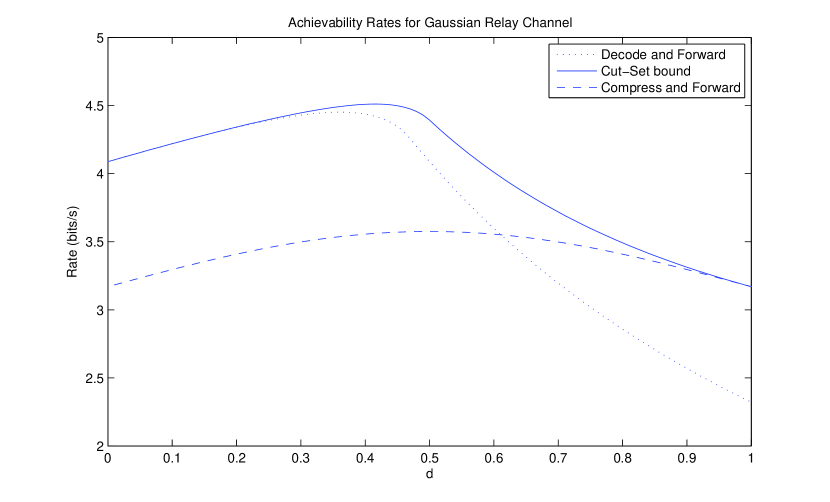
Figure 3: Achievable rates for the Gaussian relay channel, where $d$ is the normalized distance from source to relay.

Fig. 3 shows the numerical rates achievable by DF, CF and the cutset bound (14) as a function of distance $d$ of the relay from the source terminal. Depending on $d$, there are three cases:

1. When $d$ is small (roughly $d<0.2$), DF is optimal. The rate achieved by $DF$ is equal to $I(X_{1},X_{2};Y_{3})$ the multiple-access cut-set bound. The reason is that the source message can be fully decoded at the relay.

2. For medium $d$ (roughly $0.2<d<0.6$), DF is not optimal, but still performs better than CF. In this case, the rate of DF is dominated by $I(X_{1},Y_{2}|X_{2})$, the amount information can be decoded at the relay, which dictates the amount of cooperation possible between source and relay. In this region, the relay-sink channel is “poor” so that sending “finely” compressed version of $Y_{2}$ is not possible.

3. For large $d$ (roughly $0.6<d\leq 1$), CF out performs DF. In this region, the ability of the relay to decode the source is weak, and it is more fruitful to send compressed version of the relay’s observation. Only in the extreme case, $d=1$, does CF actually achieve the cut-set bound.

The rate achievable by superimposing DF and CF given by (11) is numerically compared with the rates achieved by CF, DF and the cut-set bound. The mutual information terms of (11) are evaluated for the choice of appropriate Gaussian Random variables, according to (59) and

$$I(U;Y_{2}|X_{2},V)=C\left(\frac{\frac{P_{1}}{d^{2}}\gamma^{2}(1-\alpha^{2})}{N_{1}+\frac{P_{1}}{d^{2}}(1-\gamma^{2})}\right),$$ (52)

$$I(X_{1}X_{2};Y_{3})=C\left(\frac{P_{1}+\frac{P_{2}}{(1-d)^{2}}+\frac{2\rho\sqrt{P_{1}P_{2}}}{(1-d)}}{N_{2}}\right),$$ (53)

$$I(Y_{2};\hat{Y}_{2}|U,X_{1},X_{2},Y_{3})=C\left(\frac{N_{1}}{\Delta}\right).$$ (54)

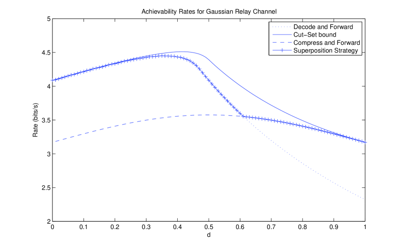
Figure 4: Achievable rates for Gaussian relay channel. The parameters of the superimposing strategy are optimized to maximize the achievable rate

The constraint $I(\hat{Y}_{2};Y_{2}|U,X_{2},Y_{3})\leq I(X_{2};Y_{3}|V)$ is evaluated to $\Delta^{\prime}\geq\Delta_{SF}$, where $\Delta_{SF}$ is as given in (51). The correlation terms $\alpha,\beta,\gamma$ and the variance $\Delta^{\prime}$ are optimizing parameters, which control the amount of information that is decoded and the amount that is compressed. When all the parameters have been optimized within the constraint posed by (51), the SF is found to achieve the maximum of $R_{DF}$ and $R_{CF}$, as shown in Fig. 4.

VI Conclusion

We analyzed the coding strategy of superimposing CF and DF for the Gaussian relay channel. We note that superposition of CF and DF does not provide higher achievable rates than the individual DF and CF for the Gaussian case. We conclude that we should look for new strategies different from superposition strategy, or look for non-Gaussian distributions for the superposition scheme, or try to find tighter upper bounds than the cut-set bound.

-A Proof of Lemma 1

Proof:

Assume without loss of generality that all three random variables are zero mean. We have

$$\begin{split}\phi_{X,Z}&=\frac{\operatorname{E}[XZ]}{\sqrt{\operatorname{E}[X^{2}]\operatorname{E}[Z^{2}]}}\\ &=\frac{\operatorname{E}\{\operatorname{E}[XZ|Y]\}}{\sqrt{\operatorname{E}[X^{2}]\operatorname{E}[Z^{2}]}}\\ &=\frac{\operatorname{E}\{\operatorname{E}[X|Y]\operatorname{E}[Z|Y]\}}{\sqrt{\operatorname{E}[X^{2}]\operatorname{E}[Z^{2}]}}\\ &=\frac{\operatorname{E}\{\sqrt{\operatorname{E}[X^{2}]/\operatorname{E}[Y^{2}]}\phi_{X,Y}Y\cdot\sqrt{\operatorname{E}[Z^{2}]/\operatorname{E}[Y^{2}]}\phi_{Y,Z}Y\}}{\sqrt{\operatorname{E}[X^{2}]\operatorname{E}[Z^{2}]}}\\ &=\phi_{X,Y}\phi_{Y,Z}\end{split}$$ (55)

∎

-B Two lemmas needed in the proof of Theorem 2

We prove two lemmas in the following that will be useful in the proof of Theorem 2. Lemma 2 is used in the case $R_{DF}\geq R_{CF}$. Lemma 3 is used in the case $R_{DF}<R_{CF}$.

Lemma 2

Let $(X_{1},X_{2},Y_{2},Y_{3},\hat{Y_{2}},U,V)$ be jointly Gaussian random variables with joint distribution $p(u,v,x_{1},x_{2},y_{2},y_{3},\hat{y_{2}})=p(v)p(u|v)p(x_{2}|v)p(x_{1}|u)p(y_{2},y_{3}|x_{1}x_{2})p(\hat{y_{2}}|y_{2},x_{2})$, where $p(y_{2},y_{3}|x_{1},x_{2})$ is as given in (4). If $I(X_{1};Y_{2}|X_{2})\geq I(X_{1};Y_{3},\hat{Y_{2}}|X_{2})$ then $I(X_{1};Y_{2}|X_{2},U)\geq I(X_{1};\hat{Y_{2}},Y_{3}|X_{2},U)$.

Proof:

Under the Gaussian assumption, we have

$$I(X_{1};Y_{2}|X_{2})=\frac{1}{2}\log\left\{1+\frac{a^{2}P_{1}(1-\rho^{2})}{N_{1}}\right\}$$ (56)

$$I(X_{1};Y_{2}|X_{2},U)=\frac{1}{2}\log\left\{1+\frac{a^{2}P_{1}(1-\gamma^{2})}{N_{1}}\right\}$$ (57)

$$I(X_{1};\hat{Y}_{2},Y_{3}|X_{2})=\frac{1}{2}\log\left\{1+P_{1}(1-\rho^{2})\frac{(N_{1}+\Delta)+a^{2}N_{2}}{(N_{1}+\Delta)N_{2}}\right\}$$ (58)

$$I(X_{1};\hat{Y}_{2},Y_{3}|X_{2},U)=\frac{1}{2}\log\left\{1+P_{1}(1-\gamma^{2})\frac{(N_{1}+\Delta)+a^{2}N_{2}}{(N_{1}+\Delta)N_{2}}\right\}$$ (59)

Obviously when $\rho=1$ and hence $\gamma=1$ (because $\rho=\alpha\beta\gamma$), the lemma holds. We thus assume that $\rho<1$. Since $I(X_{1};Y_{2}|X_{2})\geq I(X_{1};\hat{Y}_{2},Y_{3}|X_{2})$, from (56) and (57) we have

$$\frac{a^{2}P_{1}(1-\rho^{2})}{N_{1}}\geq P_{1}(1-\rho^{2})\frac{(N_{1}+\Delta)+a^{2}N_{2}}{(N_{1}+\Delta)N_{2}}.$$ (60)

Multiplying both sides with $(1-\gamma^{2})/(1-\rho^{2})$, we obtain

$$\frac{a^{2}P_{1}(1-\gamma^{2})}{N_{1}}\geq P_{1}(1-\gamma^{2})\frac{(N_{1}+\Delta)+a^{2}N_{2}}{(N_{1}+\Delta)N_{2}}.$$ (61)

It then follows that $I(X_{1};Y_{2}|X_{2},U)\geq I(X_{1};\hat{Y}_{2},Y_{3}|X_{2},U)$ from the monotonic property of the logarithmic function. ∎

Lemma 3

Let $(X_{1},X_{2},Y_{2},Y_{3},\hat{Y_{2}},U,V)$ be jointly Gaussian random variables with distribution $p(u,v,x_{1},x_{2},y_{2},y_{3},\hat{y_{2}})=p(v)p(u|v)p(x_{2}|v)p(x_{1}|u)p(y_{2},y_{3}|x_{1},x_{2})p(\hat{y_{2}}|y_{2},x_{2})$, where $p(y_{2},y_{3}|x_{1},x_{2})$ is as given in (4). If $I(X_{1};Y_{2}|X_{2})\leq I(X_{1};\hat{Y}_{2},Y_{3}|X_{2})$ then $I(U;Y_{2}|X_{2})\leq I(U;\hat{Y}_{2},Y_{3}|X_{2})$.

Proof:

Under the Gaussian variable assumptions, we have

$$I(X_{1};Y_{2}|X_{2})=\frac{1}{2}\log\left\{1+\frac{a^{2}P_{1}(1-\rho^{2})}{N_{1}}\right\}$$ (62)

$$I(U;Y_{2}|X_{2})=\frac{1}{2}\log\left\{1+\frac{a^{2}P_{1}(\gamma^{2}-\rho^{2})}{N_{1}+a^{2}P_{1}(1-\gamma^{2})}\right\}$$ (63)

$$I(X_{1};\hat{Y}_{2},Y_{3}|X_{2})=\frac{1}{2}\log\left\{1+P_{1}(1-\rho^{2})\frac{(N_{1}+\Delta)+a^{2}N_{2}}{(N_{1}+\Delta)N_{2}}\right\}$$ (64)

$$I(U;\hat{Y}_{2},Y_{3}|X_{2})=\frac{1}{2}\log\left\{1+\frac{P_{1}(\gamma^{2}-\rho^{2})[(N_{1}+\Delta)+a^{2}N_{2}]}{(N_{1}+\Delta)N_{2}+P_{1}(1-\gamma^{2})[(N_{1}+\Delta)+a^{2}N_{2}]}\right\}$$ (65)

It can be verified that when $\gamma=1$, $I(X_{1};Y_{2}|X_{2})=I(U;Y_{2}|X_{2})$ and $I(X_{1};\hat{Y}_{2},Y_{3}|X_{2})=I(U;\hat{Y}_{2},Y_{3}|X_{2})$, so that the desired result holds in this case. In the following, we assume that $\gamma<1$, and therefore $\rho=\alpha\beta\gamma<1$.

Since $I(X_{1};Y_{2}|X_{2})\leq I(X_{1};\hat{Y}_{2},Y_{3}|X_{2})$, it follows from (62) and (63) that

$$\frac{a^{2}P_{1}(1-\rho^{2})}{N_{1}}\leq\frac{P_{1}(1-\rho^{2})[(N_{1}+\Delta)+a^{2}N_{2}]}{(N_{1}+\Delta)N_{2}}.$$ (66)

Multiplying both sides of (66) with $(1-\gamma^{2})/(1-\rho^{2})$ we obtain

$$\frac{a^{2}P_{1}(1-\gamma^{2})}{N_{1}}\leq\frac{P_{1}(1-\gamma^{2})[(N_{1}+\Delta)+a^{2}N_{2}]}{(N_{1}+\Delta)N_{2}}.$$ (67)

Adding the numerator to the denominator on both sides, we obtain

$$\frac{a^{2}P_{1}(1-\gamma^{2})}{N_{1}+a^{2}P_{1}(1-\gamma^{2})}\leq\frac{P_{1}(1-\gamma^{2})[(N_{1}+\Delta)+a^{2}N_{2}]}{(N_{1}+\Delta)N_{2}+P_{1}(1-\gamma^{2})[(N_{1}+\Delta)+a^{2}N_{2}]}.$$ (68)

Multiplying both sides of (68) by $(\gamma^{2}-\rho^{2})/(1-\gamma^{2})$, we obtain

$$\frac{a^{2}P_{1}(\gamma^{2}-\rho^{2})}{N_{1}+a^{2}P_{1}(1-\gamma^{2})}\leq\frac{P_{1}(\gamma^{2}-\rho^{2})[(N_{1}+\Delta)+a^{2}N_{2}]}{(N_{1}+\Delta)N_{2}+P_{1}(1-\gamma^{2})[(N_{1}+\Delta)+a^{2}N_{2}]}$$ (69)

It then follows that $I(U;Y_{2}|X_{2})\leq I(U;\hat{Y}_{2},Y_{3}|X_{2})$ due to the monotonic property of the logarithmic function. ∎

Figure 1: Gaussian relay channel

Figure 2: Dependency graph of random variables with correlation coefficients

References

• [1] E. C. van der Meulen, “Three-terminal communication channels,” Advanced Applied Probability, vol. 3, pp. 120–154, 1971.
• [2] T. Cover and A. El Gamal, “Capacity theorems for the relay channel,” IEEE Trans. Inf. Theory, vol. 25, no. 5, pp. 572–584, May 1979.
• [3] A. E. Gamal and M. Aref, “The capacity of the semideterministic relay channel,” IEEE Trans. Inform. Theory, vol. 28, no. 3, pp. 536–536, Mar. 1982. [Online]. Available: doi:10.1109/TIT.1982.1056502
• [4] A. El Gamal, M. Mohseni, and S. Zahedi, “Bounds on capacity and minimum energy-per-bit for AWGN relay channels,” IEEE Trans. Inf. Theory, vol. 52, no. 4, pp. 1545–1561, Apr. 2006.
Refer to caption