Schrödinger equation in the space with
cylindrical geometric defect and possible application
to multi-wall nanotubes
Guilherne de Berredo-Peixoto(a),
Mikhail O. Katanaev(b),
Elena Konstantinova(a,c) and
Ilya L. Shapiro(a)
(a) Departamento de Física,
Universidade Federal de Juiz de Fora,
Juiz de Fora, CEP 36036–330, MG, Brazil
(b) Steklov Mathematical Institute, Gubkin St. 8, Moscow, 119991, Russia
(c) Instituto Federal de Educação, Ciéncia e Tecnologia do
Sudeste de
Minas Gerais (IFSEMG), Juiz de Fora, CEP 36080-001, MG, Brazil
Abstract
The recently invented cylindrical geometric space defect
is applied to the electron behaviour in the system which
can be regarded as a simplified model of a double-wall
nanotube. By solving the Schrdinger equation
in the region of space with cylindrical geometric defect
we explore the influence of such geometric defect on the
energy gap and charge distribution. The effect is
qualitatively similar to the one obtained earlier by
means of traditional simulation methods. In general, the
geometric approach can not compete with the known methods
of theoretical study of the nanostructures, such as
molecular dynamics. However it may be useful for better
qualitative understanding of the electronic properties of
the nanosystems.
1 Introduction
The theory of defects is an important part of the mathematical
physics. In particular, topological defects attract much
attention in modern condensed matter physics (see, e.g.,
[1, 2] for an introduction and recent review).
Another elegant approach in this area is the geometric theory
of defects [3, 4] (see also [5]
for the introduction), which is formulated in terms
of the notions originally developed in the theories
of gravity. The main kinds of defects which were described
in the framework of Riemann -Cartan geometry are dislocations
and disclinations. This means that the curvature and torsion
tensors are interpreted as surface densities of Frank and
Burgers vectors and thus linked to the nonlinear, generally
inelastic deformations of a solid. Recently, the qualitatively
new kind of geometric defect corresponding to the cylindrical
geometry has been described in [6].
In the framework of geometric approach, the static massive
thin cylindrical shells are considered as sources
in Einstein equations. It turns out that these defects
correspond to - and –function type
energy-momentum tensors. It would be interesting to find some
useful applications of this new kind of defect. One may
think about cosmological applications and/or about the
condensed matter physics applications, which can be not
infinitely far from each other [7].
One of the natural question to address is in which way the
new kind of defects can be applied to the condensed matter
physics? In this respect we can mention, for example,
the recent works [8, 9] devoted to the
cylindrical nanoparticles in a liquid crystal solvent.
It would be interesting to see whether the cylindric
defects can be useful in description of these systems.
However, at the first place, the cylindrical geometry is
associated with the nanotubes (see, e.g.,
[11, 10, 12, 13] for the general review).
As we shall see in what follows, the most appropriate object
of our interest would be not the usual single-wall nanotubes
but the double-wall nanotubes (DWNTs) or, more general,
multi-wall nanotubes (MWNTs).
The MWNTs attract great attention [14, 15, 16],
in particular due to higher temperature stability and
stiffness compared to the similar single-wall nanotubes.
The inner and the outer
layers of the DWNTs can be metallic (M) or semiconductor (S).
Correspondingly, there are DWNTs of different kinds, namely:
semiconductor-semiconductor (S/S case), metal-semiconductor
(M/S case), semiconductor-metal (S/M case) and metal-metal
(M/M case).
It has been emphasized recently in [17] that the
M/M type of the DWNTs is the most difficult to meet, but,
at the same time, this particular configuration is especially
interesting to explore. Let us note that there are some
theoretical and experimental data available on the energy
gap of a MWNTs compared to the purely metallic tubes
[18] (see also [15]).
In the present work we shall consider how the cylindrical
geometric defects can be related to the theoretical
investigation of the M/M type DWNTs. Our approach will
be to consider the solution of the one-particle
Schrdinger equation
in the space with the cylindrical geometric defect. Let
us note that the idea to explore the one-particle
Schrdinger equation as a way to
describe nanotubes is not completely new. One
can mention, e.g., the work of Ref. [19],
where a nonrelativistic spinless particle moving
in a cylindrical surface (also in a thick
cylindrical hollow) is investigated. On the other
side, there are also publications on quantized particles
moving in a curved background, with or without defects.
Many of them address the problem of a test particle
in a spacetime with cosmic strings and are motivated
by the corresponding cosmological models. Also, in
Ref. [20], for example, the
Schrdinger picture description of
vacuum states is studied and applied to simple
cosmological models without cosmic strings.
An important difference between the works mentioned
above and our approach is that we do not consider the
cylindrically symmetric potential. Instead, we consider the
free Schrdinger equation (without potential)
in the space with the cylindrical geometric defect. In order
to see in which situation this method may be more natural,
let us present the following observations. The conventional
nanotubes are compounds where the electron can propagate
only on the tube surface and not in the three-dimensional
bulk. In the case of DWNTs there are two distinct conducting
cylindrical shells. If we consider the electron in such
system, the tube or space division shell between the two
tubes is unlikely to create an electromagnetic potential
difference between the two conducting layers while being
essentiall for the electronic properties of the compound.
Therefore, the presence of the division between the two
shells fits the geometric defect case described in
[6], so it looks natural to perform some
investigation of the corresponding quantum systems.
It is necessary to mention some recent publications
motivated by condensed matter
applications of geometric approach. In Ref. [21],
the effect of curvature is analyzed in particle scattering.
Concerning the problems in the presence of defects, we can
also mention, e.g., Ref. [22], where a particle
which moves in a magnetic field in a space with disclination
and screw dislocation has been studied. Also, the paper
[23] explores the bounded states of an electric
dipole in the presence of a conical defect. Despite our
work can be seen as continuation of this line, we consider
a rather different approach to the geometrical defects
[6].
Indeed, there
are well-known methods for calculating electronic
and mechanic properties for different compounds, ,
or nanosystems, in particular. For example,
using the density functional (DFT) - based methods we
can explore different systems (including periodical ones),
and one obtains the desirable results with high precision
[24]. At the same time, it looks interesting to
have an alternative, more simple (albeit potentially
reliable) approach which could permit us to obtain
important qualitative information, and maybe also
help in qualitative understanding, e.g., of the electronic
properties of the mentioned systems.
In what follows we shall develop relatively
simple and to great extent analytic method based on
the geometric theory of defects. As we shall see in
brief, this approach looks justified, for it enables
one to arrive at the qualitative understanding of the
origin of modifications of energy gaps and density
distribution due to the presence of the defect shell
between the conducting layers.
The paper
is organized as follows. In the next two sections we present
a brief but to some extent pedagogical description of
the tube dislocation in the linear elasticity theory
and in the geometric theory of defects. Despite the
content of these sections is essentially the same as
the one of [6], we include it here com the
sake of completeness. In section 4 we consider the
Schrdinger
equation and describe the results of its numerical solution.
In particular, we compare the energy levels and charge
density distributions of the MWNTs with the ones of the
similar cylindrical tube without defect (it can be obtained
analytically) and with the established earlier features of
the energy spectrum of the system [15, 18].
Finally, in section 5 we draw our conclusions.
2 Tube dislocation in the linear elasticity theory
Let us start by describing the tube dislocations in the
simplest case of linear elasticity theory. Consider a
homogeneous and isotropic
elastic media as a three-dimensional Euclidean space
with Cartesian coordinates ,
where . The Euclidean metric is denoted by
. The basic variable in the
elasticity theory is the displacement vector of a
point in the elastic media, , .
In the absence of external forces, Newton’s and Hooke’s
laws reduce to three second order partial differential
equations which describe the equilibrium state of elastic
media (see, e.g., [25]),
(1)
Here is the Laplace operator and
the dimensionless Poisson ratio
() is defined as
and are called the Lame coefficients, they
characterize the elastic properties of media.
Raising and lowering of Latin indices
can be done by using the Euclidean metric, ,
and its inverse, .
Eq. (1) together with the corresponding
boundary conditions enables one to establish the
solution for the field in a unique way.
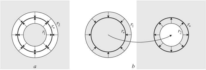
Let us pose the problem for the tube dislocation shown in
Figure 1,a.
Figure 1: Negative (a)
and positive (b) tube dislocations.
This tube dislocation can be produced as follows. We cut
out the thick cylinder of media located between two parallel
cylinders of radii and () with the axis
as the symmetry axis of both cylinders, move
symmetrically both cutting surfaces one to the other and
finally glue them. Due to circular and translational
symmetries of the problem, in the equilibrium state the
gluing surface is also the cylinder, of the radius
which will to be found below.
Within the procedure described above and shown in
Fig.1,a we observe the negative tube
dislocation because part of the media was removed. This
corresponds to the case of .
However, the procedure can be applied in the opposite
way by addition of extra media to as shown in
Fig.1,b. In
this case, we meet a positive tube dislocation and
the inequality has an opposite sign, .
It is important to note that the approach adopted here
above concerns our treatment of the division of the
shells of the DWNT as a geometric defect. Of course,
it can not be seen as a practical prescription for
building nanotubes of other objects.
Let us start by calculating the radius of the equilibrium
configuration . This problem is naturally formulated
and solved in cylindrical coordinates . Let
us denote the displacement field components in these
coordinates by . In our case,
due to the symmetry of the problem,
so that the radial displacement field can be
simply denoted as .
The boundary conditions for the equilibrium tube
dislocation are
(2)
The first two conditions are purely geometrical, and the
third one means the equality of normal elastic forces
inside and outside the gluing surface in the equilibrium
state. The subscripts “in” and “ex” denote the
displacement vector field inside and outside the gluing
surface, respectively.
Let us note that our definition of the displacement vector
field follows [5], but differs slightly from
the one used in many other references. In our notations,
the point with coordinates , after elastic
deformation, moves to the point with coordinates :
(3)
The displacement vector field is the difference between
new and old coordinates, . Indeed, we are
considering the components of the displacement vector field,
, as functions of the final state coordinates of
media points, , while in other references they are
functions of the initial coordinates, . The two
approaches are equivalent in the absence of dislocations
because both sets of coordinates and cover
the entire Euclidean space . On the contrary, if
dislocation is present, the final state coordinates
cover the whole while the initial state coordinates
cover only part of the Euclidean space lying outside the
thick cylinder which was removed. For this reason the final
state coordinates represent the most useful choice here.
The elasticity equations (1) can be easily
solved for the case of tube dislocation under consideration.
The Laplacian and the divergence in the cylindrical
coordinates have the form
(4)
(5)
where the indices are lowered using the Euclidean metric
in cylindrical coordinates,
, and .
Let us note that the last two terms in (4) are
due to the geometric covariant nature of the Laplace
operator, which is constucted on the basis of covariant
derivatives.
One can remember that only the radial component differs
from zero. The angular and components of
equations (1) are identically satisfied, and
the radial component reduces to the ordinary differential
equation,
(6)
which has a general solution
depending on the two arbitrary constants of integration
and . Due to the first two boundary conditions
(2), the solutions inside and outside the
gluing surface are
(7)
The signs of the integration constants correspond to the
negative tube dislocation shown in Fig.1,a.
For positive tube dislocation, Fig.1,b,
both integration constants have opposite signs,
and .
Using the solution (2) and the third boundary
condition (2), one can determine the radius
of the gluing surface,
(8)
After simple algebra the integration constants can be
expressed in terms of the initial radius of external and
internal cylinders
(9)
where
are the thickness of the removed cylinder and the radius of
the gluing surface, respectively. The first expression in
(9) restricts the range of the integration
constant, .
It is interesting to note that the above formulas are
applicable for both negative and positive tube dislocations.
One has to take and in these cases, respectively.
Indeed, the negative thickness in the last case means that,
before the deformation, the external radius must be smaller
than the internal one and that the proper deformation
consists in inserting some matter between the cylindrical
surfaces. In both cases we see that the gluing surface
lies exactly in the middle between the radii
and .
Finally, within the linear elasticity theory,
Eq.(7) with the integration constants
(9) yields a complete solution for the tube
dislocation. This solution is valid for small relative
displacements, when and .
It is remarkable that the solution obtained in the
framework of linear elasticity theory does not depend
on the Poisson ratio of the media. In this sense, the
tube dislocation is a purely geometric defect which
does not feel the elastic properties.
In order to use the geometric approach we have to present
the results obtained above in other terms. For this end we
compute the geometric quantities of the manifold
corresponding to the tube dislocation. From the geometric
point of view, the elastic deformation (3) is
a diffeomorphism between the given domains in the Euclidean
space. The original elastic media , before the
dislocation is made, is described by Cartesian coordinates
with the Euclidean metric . An inverse
diffeomorphism transformation induces
a nontrivial metric on , corresponding to the tube
dislocation. In Cartesian coordinates this metric has
the form
We use curvilinear cylindrical coordinates for the tube
dislocation and therefore it is useful to modify our
notations. The indices in curvilinear coordinates
in the Euclidean space will be denoted by
Greek letters , . Then the
“induced” metric for the tube dislocation in
cylindrical coordinates is111Note1
(10)
where is the Euclidean
metric written in cylindrical coordinates. We denote
cylindrical coordinates of a point before the dislocation
is made by , where without
index stands for the radial coordinate and we take into
account that the coordinates and do not
change. Then the diffeomorphism is described by a
single function relating old and new radial coordinates
of a point , where
(11)
It is easy to see that this function has a discontinuity
at the point of the cut. Therefore a special
care must be taken in calculating the components of induced
metric. It proves useful to introduce the function
(12)
which is continuous on the cutting surface. This function
differs from the derivative of the displacement
vector field defined in (11) by the
-function
(13)
Now we define the induced metric for the tube dislocation as
(14)
It is easy to check that this metric outside the cut agrees
with the expression (10). The difference between the
two expressions is that (14) is defined on the
cutting surface while (10) is not.
The volume element corresponding to (14) is
Let us note that the metric (14) differs from the
one which results from the formal substitution of
into the Euclidean metric by the
square of the -function in the component. This
procedure is required in the geometric theory of defects,
because otherwise the Burgers vector can not be expressed as
the surface integral [5]. Finally, the metric
component of tube dislocation is a
continuous function, and the angular component
has the jump at the surface of the cut.
The displacement vector field (13) and induced
metric (14) represent the solution of the field
equations of the linear elasticity theory (1)
with the boundary conditions (2) describing tube
dislocation. The solution does not depend on the elastic
properties of the media due to the universality of the
linear approximation.
3 Tube dislocation in the geometric theory of defects
Our next step is to go beyond the linear approximation and
consider the defects in elastic media with a tube dislocation.
In the geometric theory of defects
[3, 4, 27, 28]
(see [5] for the for review) the defects in
elastic media with a spin structure are the framework of
differential geometry. The main assumption is that the
elastic media is a three-dimensional manifold with a
Riemann-Cartan geometry. This approach enables one to
treat the non-linear regime and also enables one to deal
with a continuous distribution of defects.
The tube dislocation in the geometric theory of defects was
introduced and considered in details in Ref. [6],
so here we present only a short account of the formalism.
The geometry is determined by the Einstein s equations with
the source term given by the energy-momentum tensor. We
remark that the formalism under discussion is diffeomorphism
invariant and thus, in contrast to the linear elasticity
theory, the displacement vector field does not show up
explicitly in the field equations. At the same time we
require that the linear approximation gives standard result.
Therefore a natural choice for the energy-momentum tensor is
(15)
where the curvature terms are constructed by using the
metric obtained within the elasticity theory, e.g.,
(14) for the tube dislocation case. The
straighforward calculations yeild the following
relevant component of the above equation [6]:
(16)
It is worth mentioning that the above calculation is
non-trivial because the curvature terms contains
ambiguous pieces, like , but surprisingly
they cancel in the final expression.
It turns out that the solution in the geometric theory of
defects in some appropriate gauge conditions coincides
exactly with the metric (14). Thus, the result
obtained within the linear elasticity theory is quite
general and we can adopt the corresponding geometry as
a background for the quantum consideration.
4 Schrdinger equation in the
presence of tube defect
Consider the quantum description of a spinless particle
in the space with tube dislocation. The quantum properties
of our interest are encoded into the time independent
wave function, which is the solution
of the stationary covariant Schrdinger equation,
(17)
Here we use the notation , where
and are mass and energy of the particle.
is the covariant Laplacian operator, given by
(18)
Notice that the wave function behaves as a scalar field
when subject to covariant derivative, because the particle
is spinless. For this reason (18) boils down to
eq. (4) in cylindrical coordinates and, furthermore,
the torsion does not couple with the wave
function
222Note2.
The straightforward calculations lead to the following
form of Schrdinger equation in the spacetime
with the elastic deformations described in section 2,
(19)
In order to obtain the energy spectrum and density
distribution, we need to to solve the above equation
separately in the two distinct regions, namely for
(this implies also ) and
for (in this case ). We shall
denote the corresponding solutions for the wave
functions as and .
One has to take into account also the normalization
and boundary conditions, along with the matching
condition at , namely,
(20)
(21)
It would be very difficult to solve the equation
(19) in a direct way, especially outside
the tube defect. However the solution becomes rather
straightforward if we perform the inverse coordinate
transformation . In this case
the Schrdinger equation becomes very simple and in
fact it is just the one for the free particle,
(22)
After the equation (22) is solved one
has to perform the coordinate mapping, that means the
direct elasticity transformation in order to get the
solution of the equation (19) of our
interest. It is important to keep in mind that the
triviality of the equation (22) does
not mean the triviality of the solutions of the
equation of our interest (19). The
whole point is that the solutions are coordinate
dependent (while the equation is covariant) and the
physical results correspond to the coordinates
defined in eq. (3).
The solution of the free Schrdinger equation
(22) can be easily obtained via the
usual method of separating variables if we consider
a finite cylinder between and . We set
and
arrive, after replacing this form into the equation
and some standard algebra, at the solutions for
and dependences,
(23)
where and ().
These solutions correspond to the boundary conditions
. The radial function satisfies the equation
(24)
where .
The general solution for the last equation has the form
(25)
where and are Bessel function of the first
kind and of the second kind (or Neumann function)
respectively, and are arbitrary constants.
The above solution can be mapped from the “old”
coordinate into physical coordinate ,
as it was explained above, providing us an important
information on the spectrum of the system and also on
the charge density distribution. Let us discuss this in
some details.
4.1 Energy levels
Let us consider the solution of Schrdinger
equation for a particle confined in a thin region around
the geometrical defect, say, in old coordinates,
, . The two
separate solutions are
(26)
(27)
After the necessary mapping, , we arrive at
the exact solutions of the radial part of the equation
(19).
One should mention that a real finite-size tube does not
have the symmetry along the -axis, however one can
consider a very long and thin tube and thus assume the
translational -symmetry as a good approximation. In
our case this means an approximation of a large , such
that .
Consider the mapping, which was already discussed above,
in the detailed form. In what follows, we shall drop the
bars and write instead of . In order to
write down the solution in terms of physical coordinate,
we have to impose the boundary conditions in the form
(28)
These conditions give us, immediately,
and
. The last
relations must be inserted on the matching condition
at . However, it turns out that the old
matching conditions (21) are physically
unacceptable, since they imply that the charge density,
proportional to , has a discontinuity
at the surface . Thus, the following conditions
would be more appropriate:
(29)
Here we have used the expression for the volume element
in cylindric coordinates, .
Unfortunately, the above conditions provide only two
relations between arbitrary (complex) constants, in contrast
to the equations (21), which provide four relations.
Thus one should use another conditions (complex equations).
The most natural choice is continuity
of the covariant density .
Another condition with direct
physical interpretation is the current conservation, that
is the continuity of the current ,
that means ,
where
It turns out that the relations (29) or,
in a more general form,
(30)
imply the above physical assumptions and provide four
necessary relations. On the top of that we have the
normalization condition
(31)
The equations (30)
determine the discrete energy spectrum. Of course the
results are strongly dependent on the values of parameters
, , and . In order to compare the
results with the available data, let us
us specify these parameters as follows:
(32)
Typically, the outer diameter of CNT ranges between 2 and
20 nm and inner diameter ranges between 1 and 3 nm,
interlayer distance is 3.4 nm as it is established by
the high-resolution TEM techniques.
The values (32) correspond to the typical spacing
between the layers for nanotubes, confirmed, in particular,
by the experiments using diffraction and HRTEM image
techniques [30, 31]. We consider here the possibility
of describing MWNT, with several layers of carbon or other
materials. Indeed, since we are looking for a qualitative
correspondence with the results obtained by other methods,
there is no much sense in performing calculations for large
amount of possible nanotube diameters. However, since our
method is really simple, such calculation can be
easily performed, e.g., for any particular MWNT where
the fast theoretical evaluation of the effect is
needed.
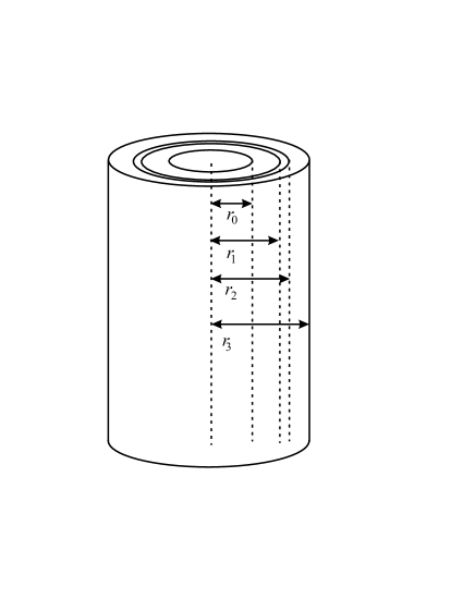
The system, as showed in Figure 2, can be
treated geometrically, by identifying nanotubes with
geometrical properties. In our consideration, a
different kind of nanotube at means a
geometrical defect at the corresponding region.
Let us note that, taking the radius magnitude close to
the ones which are typically found in nanosystems,
including MWNT’s, we also assume that the (e.g. carbon)
nanotubes layers are of the same chirality. Indeed,
one can suppose that a nanotube located at the middle,
at , has different chirality, as well as,
pehaps, few nanotubes in its vicinity [16].
Figure 2: An illustration of the general geometrical
form of a MWNT with the inner diameter of 20
and outer diameter of 200 .
Let us find the energy spectrum for the above choice, which
depends on the quantum number . We shall start from the
fundamental state, .
One can write equation (30) in terms of just
one arbitrary constant, say, , which can be fixed by
using the condition (31)). The corresponding
equation is transcendental and rather cumbersome, so it is
not convenient to write it here. The solution was performed
with the help of the software Mathematica [32].
We have found the values for which
are solutions of eq. (30). The first three
eigenvalues are placed in the left column of Table 1.
For the purpose of comparison, we put the
corresponding eigenvalues for the simplest case of the
condicting cylinder without geometrical defect, in the
right column. Similar results are presented in Table 2
for the case.
()
with defect ()
without defect ()
0.03383
0.03314
0.07016
0.06858
0.10612
0.10377
Table 1: Energy spectrum for with tube defect (left)
and without defect (right). The quantities ,
and correspond to the first three energy eigenvalues.
From these results, one can see that the tube defect does
shift, at the first place, the energy spectrum as a whole
while it almost does not change the energy gap. Still there
is a very small effect and the tendency is to reduce the
gap slightly in all cases. Similar situation occurs
for (see Table 2). This shift depends on
the size of the cutting region. In Table 3,
we put the first three energy eigenvalues for the cases
, , and , for .
Of course, corresponds to the case without defect.
The case corresponds to a negative tube dislocation
(see Figure 1b).
()
with defect ()
without defect ()
0.04009
0.03941
0.07490
0.07331
0.10982
0.10748
Table 2: Energy spectrum for with tube defect (left)
and without defect (right).
It is remarkable that the energy levels do shift under
the mapping from the “old” coordinates to the physical
ones while one could naively expect that these levels
remain the same. The reason is that (as we have already
mentioned) the mapping does not change the general
solutions of the Schrdinger equations,
while our interest is concentrated on the particular
solutions with the given boundary conditions. These
conditions do change under the mapping and this makes
the solutions of the equation (19)
really nontrivial.
()
0.03248
0.03314
0.03383
0.03456
0.06706
0.06858
0.07016
0.07183
0.10153
0.10377
0.10612
0.10858
Table 3: The three first energy levels for for the
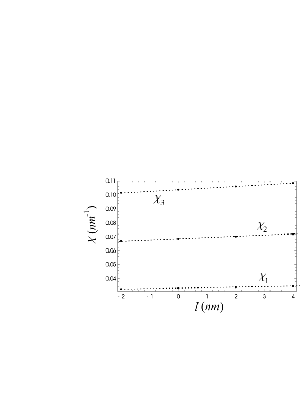
cases , , and .
How is the dependence of the energy levels
on the size ? As suggested by the data of Tables 1, 2 and 3,
positive induces a slight increase of energy
eigenvalues, while a negative lowers them. The
exact function () is unknown
and all we can do is to plot the data from Table 3
as shown in Figure 3. This plotting clearly
suggests a linear dependence between the energy levels
and the size .
Figure 3: Representation of the data of Table 3 in the plane
. The first three eigenvalues,
, and
are plotted for the cases , ,
and . The dashed lines are supposed to
describe the assumed linear dependence.
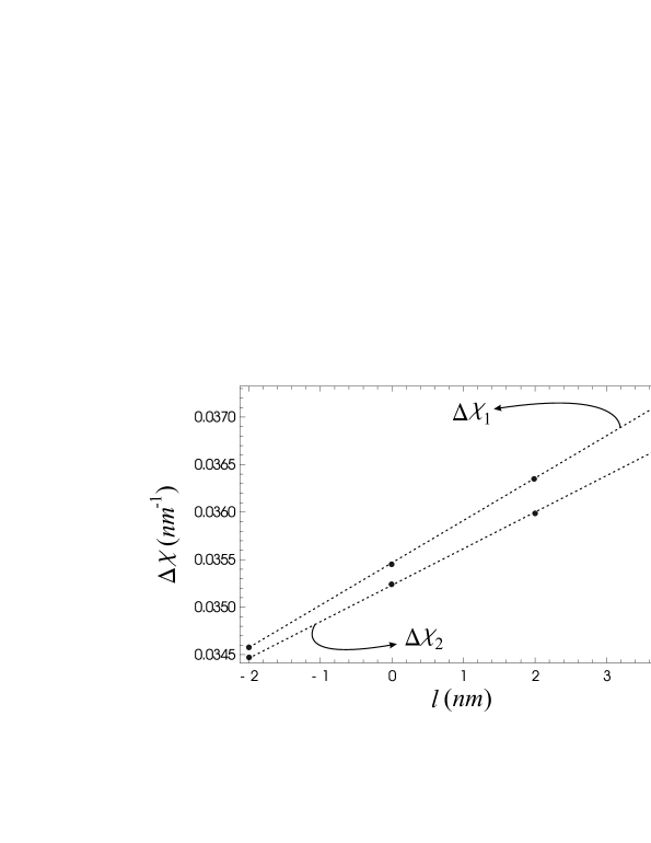
One can notice, by straighforward computation, that
the energy gaps,
and , are slightly
increased for and decreased for . For example,
for , is 4.4% greater than
the corresponding value of for .
The values of are shown in Table 4,
and are plotted in Figure 4. We can observe again
a linear relation between and . Let us notice
that, by assuming linear dependence, the straight line
describing has a lower angular
coefficient than the one corresponding to .
()
0.03458
0.03544
0.03633
0.03727
0.03447
0.03520
0.03596
0.03675
Table 4: The first two energy gaps,
and
,
for for different values of .
Figure 4: Representation of the data of Table 4 in the plane
.
The two first energy gaps,
and , are drawn for
different values of . The dashed lines are supposed to
describe the assumed linear dependence.
4.2 Density Curves
In the ideal gas approximation, the volume integral
of the density distribution,
,
is proportional to , with the
constant of proportionality having dimensions of area. From the
condition (31), has dimensions of
[length]-3 and one can find (using
Mathematica software) the following values for :
, and for ,
and , respectively,
for , with tube defect. The corresponding values without
defect, for , and are
, and
, respectively.
With these values, one can plot the normalized density against
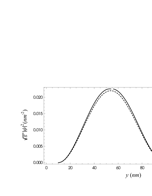
the coordinate . In Figure 5, for the lowest
energy eigenvalue, , and , the normalized density
is plotted as well as the normalized density without defect for
comparison. Notice that the curve in the presence of defect has
a cut because the point is identified with , so the
interval is formally absent in the space with
tube defect. The defect raises density in the central region.
It is interesting to observe that this is not the unique effect
caused by the defect. With the help of the Mathematica
software, one can calculate the value of for which the
density reaches its maximum value. This value is given by
for the density without
defect and for the
density with and . Thus, the defect not only
raises the density distribution, but it also drags its peak
to the left.
Let us remark that the curves describing the particle density
have not symmetry around the straight line . The
peaks of the curves in Figure 5 are localized in the
left half of the region , and not
in the middle of it. Actually, this property is essentially
related to the properties of the Bessel functions. Indeed,
let us remmember that the system is not unidimensional, such that
it does not possess symmetry around the middle point.
Figure 5: Normalized density for and .
The continuous line has a cut and describes density
in the presence of tube defect. The dashed line describes density
without defect.
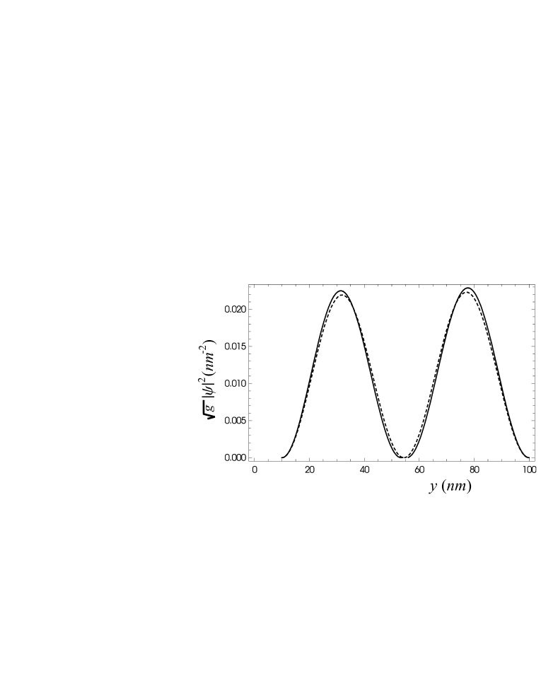
For and still , the corresponding density
curves are plotted in Figure 6. In the presence of the
tube defect, the density is lower in central region but greater
in the marginal regions, and .
The shifts in the density distribution
are small and of the same order in both cases, and
, but in the last case the difference is richer. In the
central region, the defect raises the density for
and lowers the density for . Of course, for a larger
, these effects may become much more sensitive.
Figure 6: Normalized density for and .
The continuous line has a cut and describes density
in the presence of tube defect. The dashed line describes density
without defect.
5 Conclusions
We considered the solution of the Schrdinger
equation in the restricted region of space with cylindrical
geometric defect. The region is confined between the two
cylindrical shells and the diameter of the defect is
intermediate between the ones of these shells.
Geometrically this configuration resembles the double-wall
nanotube (DWNT) and, therefore, it can be regarded as a simplified
model of such nanotube. Due to the fact that the electron
can freely move within the space between the two border
shells, one can associate the system with the M/M-type
DWNT. The solution of the Schrdinger equation
shows the influence of the geometric defect on the energy
gap and charge distribution. In particular, one meets a
modified energy spectrum and the distribution of charge
density, in the ideal gas approximation. These effects
are qualitatively similar to the ones previously reported for
some MWNTs in [18], where the calculations were based
on the tight-binding method. In this respect we can conclude
that the approach based on geometric defects, which does
not take into account anything but the general form of the
DWNT, is able to provide some (very restricted, indeed)
information about the electron behaviour.
It is obvious that the method based on geometric defects
can not compete with the standard approaches based on
molecular dynamics. The reason is that the geometric
defects method can not take into account full details
of the structure of the compound and is, in some sense,
too general. At the same time this method may become much
more interesting if one develops it further and, in particular,
learns how to deal with more sophisticated versions of
geometric defects. In particular, it looks possible to
take into account the chirality of the nanotube and,
also, include the external magnetic field. We expect to
consider these issues elsewhere.
Acknowledgments
G.B.P., E.K. and I.Sh. are indebted to CNPq, FAPEMIG and
FAPES for partial support. M.K. is thankful to FAPEMIG for
support of his visit to Brazil and to the Physics Department
of the Universidade Federal de Juiz de Fora for warm
hospitality. Also, he thanks the Russian
Foundation of Basic Research (Grant No. 08-01-00727), and
the Program for Supporting Leading Scientific Schools
(Grant No. NSh-3224.2008.1) for financial support.
The work of I.Sh. has been also supported by ICTP.
References
[1] P.M. Chaikin and T.C. Lubensky,
Principles of Condensed Matter Physics.
(Cambridge University Press, Cambridge, 2000).
[2]
M. Kleman and J. Friedel, Rev. Mod. Phys. 80 (2008) 61.
[3]
M. O. Katanaev and I. V. Volovich.
Theory of defects in solids and three-dimensional gravity.
Ann. Phys., 216(1):1–28, 1992.
[4]
M. O. Katanaev and I. V. Volovich.
Scattering on dislocations and cosmic strings in the
geometric theory of defects.
Ann. Phys., 271: 203–232, 1999.
[5]
M. O. Katanaev.
Geometric theory of defects.
Physics – Uspekhi,
48(7):675–701, 2005.
[6] G. de Berredo-Peixoto and M. O. Katanaev,
Tube dislocations in gravity, J. Math. Phys. 50: 042501, 2009.
[7]
W.H. Zurek, Physics Reports, 276 (1996) 177;
T. W. B.Kibble and G.R. Pickett,
Philosophical transactions of the Royal Society A -
Mathematical, Physical and Engineering Sciences,
366 (2008) 2793.
[8] M. Das, A. Vaziri, A. Kudrolli, and L. Mahadevan,
Curvature Condensation and Bifurcation in an Elastic Shell,
Phys. Rev. Lett. 98: 014301, 2007.
[9] D.L. Cheung and M.P. Allen,
Forces between Cylindrical Nanoparticles in a Liquid Crystal
Langmuir, 24 (2008) 1411.
[10] T.W. Ebbesen (Editor),
Carbon Nanotubes. Preparation and Properties.
CRC Press, Boca Raton New York London Tokyo, 1997.
[11]
R. Saito, G. Dresselhaus and M.S. Dresselhaus,
Physical Properties of Carbon Nanotubes,
(Imperial College, London, 1998).
[12] P.J.F. Harris,
Carbon Nanotubes and Related Structures: New
Materials for the Twenty-First Century,
(Cambridge University Press, 1999).
[13]
M. S. Dresselhaus, G. Dresselhaus and P. Avouris (Editors),
Carbon Nanotubes : Synthesis, Structure, Properties,
and Applications, (Springer-Verlag, 2000).
[14]
A. M. Fennimore, T. D. Yuzvinsky, Wei-Qiang Han, M. S.
Fuhrer, J. Cumings, A. Zettl,
Rotational actuators based on carbon nanotubes,
Nature 424 (2003) 408; A. Modi, N. Koratkar, E. Lass, B. Wei, P.M. Ajayan,
Miniaturized gas ionization sensors using carbon
nanotubes,
Nature 424 (2003) 171; M. Zhang, S. Fang, A.A. Zakhidov, S.B. Lee, A.E. Aliev,
C.D. Williams, K.R. Atkinson, and R.H. Baughman,
Strong, Transparent, Multifunctional, Carbon
Nanotube Sheets,
Science 309 (2005) 1215; R.H. Baughman, A.A. Zakhidov, and W.A. de Heer,
Carbon Nanotubes–the Route Toward Applications,
Science 297 (2002) 787;
[15] T. Shimada, T. Sugai, Y. Ohno, S. Kishimoto,
T. Mizutani, H. Yoshida, T. Okazaki and H. Shinohara,
Appl. Phys. Lett. 84 (2004) 2412.
[16]
Z. Xu, X. Bai, Z.L. Wang and E. Wang,
Multiwall Carbon Nanotubes Made of Monochirality
Graphite Shell,
J. Am. Chem. Soc. 128 (2006) 1052.
[17] F. Villalpando-Paez, H. Son, D. Nezich,
Y.P. Hsieh, J. Kong, Y.A. Kim, D. Shimamoto, H. Muramatsu,
T. Hayashi, M. Endo, M. Terrones and M.S. Dresselhaus,
Nano Lett. 8 (2008) 3879.
[18]
Y. H. Ho, G. W. Ho, S. J. Wu, and M. F. Lin,
J. Vac. Sci. Technol. B 24(3) (2006) 1098.
[19] J. Gravesen, M. Willatzen and
L. C. Lew Yan Voon, J. Math. Phys. 46: 012107, 2005.
[20] D. V. Long and G. M. Shore, Nucl. Phys.
B 530: 247-278, 1998.
[21] A. Mostafazadeh, Phys. Rev. A 54:
1165-1170, 1996.
[22] S. Azevedo, Mod. Phys. Lett.
A 17: 1263-1268, 2002.
[23] C. A. L. Ribeiro, C. Furtado and F. Moraes,
Mod. Phys. Lett. A 20: 1991-1996, 2005.
[24]
P. Hohenberg, W. Kohn, Phys. Rev., 136 (1964) B864;
W. Kohn, L.J. Sham, Phys. Rev., 140 (1965) A1133;
W. Kohn, M.C. Holthausen,
A Chemist s Guide to Density Functional Theory,
(WILEY-VCH, Second Edition, 2001).
[25]
L. D. Landau and E. M. Lifshits.
Theory of Elasticity.
Pergamon, Oxford, 1970.
[26] We put the
word “induced” in inverted commas because on the
cutting surface the induced metric is not defined.
[27]
M. O. Katanaev.
Wedge dislocation in the geometric theory of defects.
Theor. Math. Phys., 135(2):733–744, 2003.
[28]
M. O. Katanaev.
One-dimensional topologically nontrivial
solutions in the Skyrme model.
Theor. Math. Phys., 138(2):163–176, 2004.
[29] Both features may not hold in the spinning
particle case, which becomes relevant for the more
general types of tube geometric defects.
[30] T.W. Ebbesen (Editor),
Carbon Nanotubes. Preparation and Properties.
(CRC Press, Boca Raton, 1997),
see especially Chapter 3 therein,
P.M. Ajayan,
Structure and Morphology of Carbon Nanotubes.
[31]
M.S. Dresselhaus, G. Dresselhaus and P.C. Eklund,
Science of Fullerens and Carbon Nanotubes,
(Academic Press, San Diego, 1996), see especially
the data in Chapter 19.
[32] S. Wolfram, The Mathematica Book
(Cambridge Univ. Press, 1999), the M6 version has
been used here.