Modelling the shapes of the largest gravitationally bound objects

Abstract

We combine the physics of the ellipsoidal collapse model with the excursion set theory to study the shapes of dark matter halos. In particular, we develop an analytic approximation to the nonlinear evolution that is more accurate than the Zeldovich approximation; we introduce a planar representation of halo axis ratios, which allows a concise and intuitive description of the dynamics of collapsing regions and allows one to relate the final shape of a halo to its initial shape; we provide simple physical explanations for some empirical fitting formulae obtained from numerical studies. Comparison with simulations is challenging, as there is no agreement about how to define a non-spherical gravitationally bound object. Nevertheless, we find that our model matches the conditional minor-to-intermediate axis ratio distribution rather well, although it disagrees with the numerical results in reproducing the minor-to-major axis ratio distribution. In particular, the mass dependence of the minor-to-major axis distribution appears to be the opposite to what is found in many previous numerical studies, where low-mass halos are preferentially more spherical than high-mass halos. In our model, the high-mass halos are predicted to be more spherical, consistent with results based on a more recent and elaborate halo finding algorithm, and with observations of the mass dependence of the shapes of early-type galaxies. We suggest that some of the disagreement with some previous numerical studies may be alleviated if we consider only isolated halos.

1 Introduction

A snapshot of a high-resolution dark matter simulation, at relatively low redshift, reveals that halos are neither spherically symmetric nor smooth. This is because, without even considering all the small scale complications arising from baryonic physics (i.e. pressure effects, merging, cooling, heating), the statistics of a Gaussian random field implies that spherically symmetric initial configurations should be a set of measure zero (Doroshkevich 1970). While it has long been recognized that spherical collapse is too idealized to be realistic, and that the true gravitational process must, at the very least, be ellipsoidal (Icke 1973; White & Silk 1979; Barrow & Silk 1981; Kuhlman et al. 1996), most analytic models of structure formation make the simplifying assumption that gravitationally bound objects are spherical, and formed from a spherical collapse (i.e. Gunn & Gott 1972; Lahav et al. 1991; Lacey & Cole 1993; Lokas & Hoffman 2001).

It has also become common practice to identify halos in simulations using a spherical overdensity algorithm, which finds the mass around isolated peaks in the density field such that the mean interior density is $\Delta$ times the background density, where the value of $\Delta$ is motivated by the spherical top-hat model (Lacey & Cole 1994). This is despite the fact that dark matter halos that form in simulations are rather elongated, and, in general, strongly triaxial: close to prolate (minor and intermediate axes are comparable in size to each other, and much smaller than the biggest axis) in the central parts, and rounder in the outskirts (Barnes & Efstathiou 1987; Frenk et al. 1988; Dubinski & Carlberg 1991; Katz 1991; Warren et al. 1992; Jing et al. 1995; Thomas et al. 1998; Jing & Suto 2002; Allgood et al. 2006; Bett et al. 2007; Diemand, Kuhlen & Madau 2007; Hayashi et al. 2007; Kuhlen et al. 2007; Muñoz-Cuartas et al. 2010; Wang et al. 2010). This shape variation leads to a significant variance in local properties, compared to the spherically averaged value at a given radius, that are now becoming of interest.

Studying and quantifying the degree of halo triaxiality is of broader importance. In fact, in the current paradigm of hierarchical clustering, dark matter halos are the hosts within which gas cools and collapses to form galaxies (White & Rees 1978; White & Frenk 1991), thus making them the building blocks of the large scale structure (LSS) of the Universe (Cooray & Sheth 2002). Hence, understanding the assembly histories, kinematics, clustering, and fundamental structural properties of halos – such as their intrinsic shapes – is the first necessary step in understanding the properties of galaxies (Mo, Mao & White 1998; Dutton et al. 2007; Diemand et al. 2008). In turn, the formation of dark matter halos affects the properties of the galaxies hosted by the halos; therefore, inspection of the galaxy distribution in redshift surveys such as the SDSS (York et al. 2000) allows one to relate the properties of galaxies to those of their host halos. Moreover, the characteristic density of a halo appears to track the mean density of the Universe at the time of its formation (e.g. Zhao et al. 2009), leading to a quasi-universal profile (Navarro, Frenk & White 1996; Kormendy & Freeman 2004), although self-similarity is not preserved: different halos cannot be rescaled to look alike (Navarro et al. 2004, 2010; Merritt et al. 2006; Gao et al. 2008; Reed et al. 2010).

Triaxiality also has a number of observationally relevant implications. For example, modeling of dark matter halos beyond the spherical approximation is crucial in understanding the nonlinear clustering of halos and dark matter (Sheth, Mo & Tormen 2001), the formation and evolution of galaxies (Cole & Lacey 1996), and their relation to the cosmic web (Shen et al. 2006; Hahn et al. 2007; Lee, Hahn & Porciani 2009a,b; Forero-Romero et al. 2009; Pogosyan et al. 2009; Sousbie et al. 2009; Park, Kim & Park 2010). In particular, the higher order statistics of the nonlinear density field is sensitive to halo triaxiality (Smith & Watts 2005; Smith, Watts & Sheth 2006).

Triaxiality represents a useful framework for the non-spherical modelling of the intracluster gas, which recent observations suggest will be key in deriving more accurate temperature profiles of X-ray clusters, and in general for cosmological parameter determinations via the Sunyaev-Zeldovich effect (Lee et al. 2005). For example, Kawahara (2010) has derived the axis ratio distribution of X-ray clusters in the XMM-Newton catalog of Snowden et al. (2008) and confirmed that the typical X-ray halo is well approximated by a triaxial ellipsoid. And recently, Morandi, Pedersen & Limousin (2010) have presented the first determination of the intrinsic triaxial shapes and three-dimensional physical parameters of both dark matter and the intra-cluster medium for the galaxy cluster Abell 1689.

Triaxiality is also useful in predicting – and hence can be constrained by – a variety of gravitational lensing observations, including weak and strong lens statistics (Bartelmann 1995; Van Waerbeke et al. 2000; Schulz et al. 2005; Bradač et al. 2006; Carbone et al. 2006; Bernstein 2007; Riquelme & Spergel 2007; Broadhurst et al. 2008; Limousin et al. 2008; Schneider & Er 2008; Mandelbaum et al. 2008, 2009; Zitrin et al. 2009; Bernstein & Nakajima 2009; Jönsson et al. 2010), and gravitational flexion (e.g., Hawken & Bridle 2009). By measuring the shapes of dark matter halos, galaxy-galaxy lensing can provide constraints on galaxy formation models and the nature of dark matter (Hoekstra et al. 2004; Mandelbaum et al. 2006; Parker et al. 2007).

Surveys like ESA’s Euclid mission (http://sci.esa.int/euclid) will in fact provide accurate data for shape estimates through “cosmic shear”, a direct measure of the metric fluctuations in the Universe (Hoekstra & Jain 2008; Bernstein 2010; Rhodes et al. 2010), which in turn constrain dark energy properties (Albrecht et al. 2006). A primary source of noise in such measurements is due to the difficulty in distinguishing between intrinsic galaxy shapes and shape distortion due to lensing (Bartelmann & Schneider 2001; Refregier 2003; Hoekstra et al. 2005; Mandelbaum et al 2006; Bridle et al. 2009). Hence accurate modelling of the correlated shapes and orientations dark matter halos can be extremely useful. The higher order statistics of the nonlinear density field in such surveys is also sensitive to halo triaxiality (Smith et al. 2006).

On galaxy mass scales, an understanding of halo triaxiality provides useful input to studies of galactic disks in triaxial halos. E.g., Jeon, Kim & Ann (2009) considered the fundamental dynamics between the disk and the axisymmetric or triaxial halo, and Valluri et al. (2010) analyzed the orbital structure of dark matter particles in $N$-body simulations in an effort to understand what is the physical mechanism driving shape changes caused by growing central masses (also see Debattista et al. 2008). This shape change reconciles the strongly prolate-triaxial shapes found in collisionless $N$-body simulations with observations, which generally find much rounder halos (see for example Banerjee & Jog 2008). Finally, resolving the fine grained structure of galaxy mass halos enables one to make more realistic predictions for direct and indirect dark matter detection experiments (e.g. Giocoli, Pieri & Tormen 2008).

The shapes of dark matter halos can be quantified using high-resolution $N$-body simulations of hierarchical gravitational clustering. This is currently the best way to address many of the tasks above. Simulations are becoming increasingly accurate in mass and spatial resolution: e.g., the Millennium Run (Springel et al. 2005), the Horizon Run (Kim et al. 2009), the Millennium II (Boylan-Kolchin et al. 2009) and the Bolshoi Simulation (Klypin et al. 2010).

In these numerical studies, many different aspects have been considered over a wide range of physical scales and cosmic histories. Common findings suggest that the total mass is the key in determining the final shapes of halos, although other environmental parameters may play a role in the process. In general, halos do exhibit a rich variety of shapes with a preference for prolateness over oblateness. More massive halos tend to be less spherical and more prolate, and are preferentially aligned with primordial filaments, while less massive halos are in general rounder (e.g., Jing & Suto 2002; Allgood et al. 2006; Araya-Melo et al. 2009). On the other hand, perturbation theory suggests that the most massive objects should be spherical (Bernardeau 1994; Pogosyan et al. 1998), and Lemson (1995) showed that the spherical model does provide a good description of the evolution of the spherically averaged profile. More recently, Dalal et al. (2008) reported that massive halos are indeed very well described by the spherical collapse model. This was recently confirmed by Park et al. (2010), who provided a clear explanation for the discrepancy with previous measurements.

The shapes of subhalos are similar to those of host halos, but subhalos tend to be a bit rounder, especially the ones near the host halo center. Tidal interactions make individual subhalos rounder over time and they tend to align their major axis towards the center of the host halo. Formation of halos is also affected by the large-scale environment, which may have an impact on their shapes, and those shapes can be modified by galaxy formation as well. Subhalos are not the subject of our study.

There are many more numerical studies of halo shapes than analytic models. This is because the formation, evolution and virialization of dark matter halos is complex; no rigorous analytic techniques are available for use in both the linear and the nonlinear regimes. In addition, choosing the appropriate definition of halo shapes is subtle. For example, Eisenstein & Loeb (1995) describe an analysis of halo shapes which uses the ellipsoidal collapse model of Bond & Myers (1996). However, as we discuss below, their definition of a halo differs from the more commonly accepted definition. Moreover, they present results for collapsed objects that had the same initial density. Since the time it takes for to collapse is a complicated function of density and shape (Bond & Myers 1996), this means that they compare objects of one shape at one time with those of another shape at a different time. This is rarely measured in simulations: the shape distribution of most interest is, of course, that for a fixed time (e.g., halos at $z=0$).

The main purpose of the present work is to provide a simple model for the distribution of halo shapes at any given time as seen in the simulations, starting from first principles. Following Rossi (2008), our analytic prescription has two independent parts: the first is a scheme for how an initially spherical patch evolves and virializes; the second is the correct assignment of initial shapes to halos of different masses.

In this respect, our model is similar in philosophy to that of Lee, Jing & Suto (2005). However, there are important differences. (1) They assume the Zeldovich approximation remains valid even during the nonlinear regime, where it is known to fail; (2) They assume a spherical collapse threshold for the formation of halos, or an empirical recipe based on Lee & Shandarin (1998). In contrast, because we are modelling triaxial objects, we self-consistently use ellipsoidal, rather than spherical collapse dynamics to generate our predictions.

To describe the evolution of non-spherical structures we adopt the ellipsoidal collapse model of Bond & Myers (1996), which was used by Sheth, Mo & Tormen (2001) to estimate of how the abundance of dark matter halos depends on halo mass. In this model, dark matter halos are identified with ellipsoids which have collapsed completely along all three axes (we show below that, in effect, the Eisenstein & Loeb 1995 definition corresponds to collapse along just two axes). In this framework, the time required to collapse depends on the overdensity $\delta_{\rm i}$ and size $R_{\rm i}$ of the initial patch, and on the surrounding shear field, parametrized by its ellipticity $e$ and prolateness $p$. Requiring the collapse to happen at a given time makes $\delta_{\rm i}$ a function of $e$ and $p$ (Sheth et al. 2001): $\delta_{\rm ec}(e,p)$. The combination of $\delta_{\rm i}=\delta_{\rm ec}$, $e$ and $p$ determines the axis ratios of the object at all times, and, in particular, at the final time. Thus ($e,p$) establishes the time of collapse (it was this fact which was exploited by Sheth et al. 2001), as well as the axis ratios at collapse (a fact we exploit here).

The second part is the correct assignment of ($e,p$) values to halos of different masses. We do this following Sheth & Tormen (2002) (also see Chiueh & Lee 2001; Sandvik et al. 2007). In essence, the correct ($e,p$) distribution is specified by the statistics of Gaussian random fields. In a Gaussian random field, the distribution of ($e,p$) values depends on the size and overdensity of the patch: $g(e,p|\delta,R)$. Massive halos form from larger patches in the initial conditions than do less massive halos, so we expect the distribution of initial ($e,p$) values, and hence the distribution of final axis ratios, to also depend on halo mass. Thus, although the generic evolution is initially towards an oblate, pancake-like structure, followed by a shift towards a more prolate shape, as the other axes also begin to shrink, quantifying this evolution, and merging it with the correct (mass dependent) initial distribution of shapes is the main focus of this work.

The outline of this paper is as follows. In Section 2 we present the ellipsoidal model for the gravitational collapse of an initially spherical patch; we discuss a reasonably accurate analytic approximation to the evolution, more rigorous than the Zeldovich approximation; we introduce the axis ratio plane, which provides a concise description of the dynamics of collapsing regions and allows one to relate the final shape of a halo with its original, pre-collapsed, shape. In Section 3 we present the full model for halo shapes, we explain how the initial conditions are obtained via the excursion set algorithm, and we expand on the prolateness distribution – crucial in understanding our main results. In Section 4 the model is contrasted with high resolution $N$-body simulations. A simple explanation of an empirical relation found by Jing & Suto (2002) is given, and a number of caveats in the comparison model/simulations are highlighted. Finally, Section 5 discusses in detail limitations in the modelling and difficulties arising from numerical studies, and suggests future improvements.

In our calculations we assume a spatially flat cosmological model with $(\Omega_{\rm M},\Omega_{\rm\Lambda},h)=(0.3,0.7,0.7)$, where $\Omega_{\rm M}$ and $\Omega_{\rm\Lambda}$ are the present day densities of matter and cosmological constant scaled to the critical density. We write the Hubble constant as $H_{0}=100h$ km s^-1 Mpc^-1. Regarding the overall notation, we always use the subscript $i$ to denote initial quantities, and the subscript $f$ for final quantities. The expansion factor of the Universe, with mean density $\bar{\rho}$, is represented by the small case letter $a$ – not to be confused with the capital letter $A$, which denotes the axis ratios of an ellipsoidal patch.

2 Nonlinear dynamics

The nonlinear gravitational evolution of a medium is complex, even without complications arising from gas dynamics. It involves smooth accretion, tidal interactions with the environment as well as violent episodes of collisions with other halos, merging and fragmentation. In what follows, we first briefly summarize the key aspects of the ellipsoidal collapse. We then discuss an analytic approximation for the evolution, and introduce a planar representation of halo axis ratios; this allows for a concise description of the dynamics of collapsing regions, and provides a mapping between the initial and final shape of a halo.

2.1 A model for the gravitational collapse

The simplest description of the gravitational evolution and virialization of a cosmic structure is the spherical collapse model (Gunn & Gott 1972; Gott 1975; Gunn 1977; Fillmore & Goldreich 1984; Bertschinger 1985; Mo & White 1996). In this framework, an isolated overdensity in an otherwise unperturbed universe first expands with the Hubble flow, then turns around and collapses. However, the initial shear field, rather than the density, has been shown to play a crucial role in the formation of nonlinear structures (Zeldovich 1970; Hoffman 1986, 1988; Peebles 1990; Dubinski 1992; van de Weygaert & Babul 1994; Audit & Alimi 1996; Audit, Teyssier & Alimi 1997). Therefore, refinements to the spherical approximation which include local shear effects can be obtained by introducing an ellipsoidal collapse scheme (Bond & Myers 1996; Eisensein & Loeb 1995; Monaco 1995, 1997, 1998; Lee & Shandarin 1998; Chiueh & Lee 2001; Sheth, Mo & Tormen 2001; Sheth & Tormen 2002; Ohta et al. 2004; Shen et al. 2006; Sandvik et al. 2007; Desjacques 2008; Desjacques & Smith 2008; Rossi 2008).

In this study we adopt the homogeneous ellipsoidal model in the form of Bond & Myers (1996), although the ellipsoidal collapse has a long history (Lin, Mestel & Shu 1965; Icke 1973; White & Silk 1979; Barrow & Silk 1981). To lowest order, their algorithm reduces to Zeldovich’s (1970) approximation, and so linear theory is reproduced. In this framework, an initially spherical patch of initial size $R_{\rm i}$ with overdensity $\delta_{\rm i}$ is distorted by the shear field into a collapsing homogeneous ellipsoid. The exterior tidal force arising from the matter outside of the ellipsoid is completely determined by the volume-averaged strain of the ellipsoid. The details of the substructure in the interior are ignored, and the strongly nonlinear internal dynamics of the collapsing patch are assumed to be largely decoupled from the weakly nonlinear dynamics describing the motion of the patch itself; in this respect, the homogeneous ellipsoid picture may be thought of as a tensor virial theorem approach to the average interior dynamics. In fact, in the nonlinear regime the one-to-one correspondence between the external tidal field and the local strain tensor is no longer true on small scales where the rms density fluctuation $\sigma\gg 1$; therefore, one would not expect the simple ellipsoidal model to apply in this regime.

There is another sense in which this approach is only a simple approximation. It assumes that the inertia tensor of the final bound object is perfectly correlated with the local tidal tensor in the initial Lagrangian space. Measurements in simulations show that the two tensors are not perfectly correlated (e.g. Lee & Pen 2000). On the other hand, the correlation is stronger than naive tidal torque theories predict (e.g., Porciani, Dekel & Hoffman 2002), so the assumption of perfect correlation is a useful idealization.

It is usual to characterize the initial shear field by the ellipticity $e$ and prolateness $p$ associated with the potential rather than with the density field (i.e. Bardeen et al. 1986). This is because the components of the $3\times 3$ strain tensor are the second derivatives of the potential. The eigenvalues of the initial strain tensor are related to the initial density contrast and to the shear ellipticity and prolateness by:

$$\lambda_{1}(t_{\rm i})={\delta(t_{\rm i})\over 3}(1+3e+p),$$ (1)

$$\lambda_{2}(t_{\rm i})={\delta(t_{\rm i})\over 3}(1-2p),$$ (2)

$$\lambda_{3}(t_{\rm i})={\delta(t_{\rm i})\over 3}(1-3e+p).$$ (3)

Note that $\sum_{\rm j}\lambda_{\rm j}=\delta_{\rm i}$. If $\delta>0$, then $e\geq 0$ and $-e\leq p\leq e$, so $\lambda_{1}\geq\lambda_{2}\geq\lambda_{3}$.

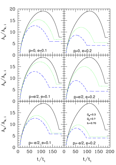
Figure 1: Evolution of axis lengths in our model, in physical units. The times at which different axes freeze out are determined by the initial ($e,p,\delta$) values, as specified in the panels.

If we denote with $A_{\rm k}$ the scale factors for the three principal axes of the ellipsoid, then the initial conditions are set by the Zeldovich approximation, both for the displacement and the velocity fields:

$$A_{\rm k}(t_{\rm i})=a(t_{\rm i})[1-\lambda_{\rm k}(t_{\rm i})],$$ (4)

$${{\rm d}A_{\rm k}(t_{\rm i})\over{\rm d}t}=H(t_{\rm i})\Big{[}A_{\rm k}(t_{\rm i})-a(t_{\rm i})\lambda_{\rm k}(t_{\rm i}){{\rm d~{}ln}D\over{\rm d~{}ln}a}\Big{|}_{\rm t\equiv t_{\rm i}}\Big{]}.$$ (5)

Notice that $A_{3}\geq A_{2}\geq A_{1}$. The subsequent evolution is given by

$$\frac{{\rm d}^{2}A_{\rm k}}{{\rm d}t^{2}}=\Omega_{\rm\Lambda}H_{0}^{2}A_{\rm k}-4\pi G\bar{\rho}A_{\rm k}\Big{[}\frac{1+\delta}{3}+\frac{b^{\prime}_{\rm k}\delta}{2}+\lambda^{\prime}_{\rm ext,k}\Big{]},$$ (6)

where $\bar{\rho}$ is the mean density of the Universe, $\delta$ the relative overdensity, and $b^{\prime}_{\rm k}=b_{\rm k}-2/3$ and $\lambda^{\prime}_{\rm ext,k}$ account for the interior and exterior tidal forces. In particular,

$$b_{\rm k}(t)=\Big{[}\prod_{\rm m=1}^{\rm 3}A_{\rm m}(t)\Big{]}\int_{0}^{\infty}{{\rm d}\tau\over[A_{\rm k}^{2}(t)+\tau]\prod_{\rm j=1}^{3}[A_{\rm j}^{2}(t)+\tau]^{\rm 1/2}}$$ (7)

and

$$\lambda^{\prime}_{\rm ext,k}(t)=\frac{D(t)}{D(t_{\rm i})}\Big{[}\lambda_{\rm k}(t_{\rm i})-\delta(t_{\rm i})/3\Big{]},$$ (8)

with $D$ the linear theory growing mode. Other possibilities for $\lambda^{\prime}_{\rm ext,k}$ include the ‘nonlinear’ (Bond & Myers 1996), or the ‘hybrid’ (Angrick & Bartelmann 2010) approximations. However, in our case we are concerned with later times, where a different choice for the external shear field does not significantly affect our conclusions.

If $e=p=0$, then all three eigenvalues equal $\delta_{\rm i}/3$, hence all three axes have the same length initially. In this case, the exterior anisotropic tidal force is zero and $b^{\prime}_{\rm k}=0$, so one gets the usual cycloid solution for a closed universe. Hence, all three axes evolve similarly, so the object remains spherical, and the time to collapse is determined by one number: $\delta_{\rm i}$. But for more general initial values of $\delta(t_{\rm i})$, $e$ and $p$, and an initial redshift, equation (6) must be solved numerically for each axis $A_{\rm k}$. Generically, a triaxial object has three critical times, corresponding to the collapse along each of the three axes. In this case, the shortest axis, $A_{1}$, collapses first and $A_{3}$ collapses last.

Figure 1 shows how the lengths of the three axes evolve in the model, in physical units. In all cases we set $\delta(t_{\rm i})=[D(t_{\rm i})/D(t_{\rm 0})]\delta(t_{0})$, with $\delta(t_{0})=1.6753$ being the usual critical value associated with spherical collapse in the adopted cosmology at $z=0$. Our numerical calculations start at a time $t_{\rm i}$, which corresponds to a redshift $z_{\rm i}=39$. Each panel show results for a different pair of ($e,p$). For a given $e$, $p>0$ implies a pancake-like structure (i.e. one short axis and two long), while $p<0$ results in filament-like structures. The main point of the figure is to illustrate that, in this model, a given pair ($e,p$) determines the axis ratios of the object at all times, and, in particular, at the final time.

Halos are identified with objects that have collapsed along all three axes. Bond & Myers (1996) stop collapse along axis $k$ by simply freezing $A_{\rm k}$ once a critical radius $A_{\rm eq,k}=a\,f_{\rm r}$ is reached during the infall phase, where $a$ is the expansion factor of the Universe and typically the radial freeze-out factor $f_{\rm r}=0.177$ is chosen in order to reproduce the ‘virial’ density contrast of $\Delta=a^{3}/(A_{1}A_{2}A_{3})=179$ familiar from spherical top-hat calculations in an Einstein-de Sitter model; $f_{r}$ must be computed for more complicated cosmologies.

In our study, we slightly modify the stop criterion proposed by Bond & Myers (1996) as follows: we still freeze the value of axis $i$ once a critical radius is reached during the infall phase (the radial freeze-out factor being chosen in order to reproduce the correct spherical virial density contrast in the assumed cosmological model), but we progress the evolution in time till we reach the point in which each axis has collapsed completely, in order to consider fully relaxed halos. Bond & Myers (1996) found that the time at which the longest axis of the ellipsoid freezes out is relatively insensitive to the exact value of $f_{\rm r}$, within a given cosmological model. In this respect, a more sophisticated collapse criterion such as the one recently proposed by Angrik & Bartelmann (2010), and based on the tensor-virial theorem, does not affect our analysis.

However, this stop criterion is rather different from that used by Eisenstein & Loeb (1995), and this difference does matter. In their prescription, the collapse is stopped at the time when a sphere, whose overdensity was that of the initial ellipsoid, would have shrunk to zero radius. This happens to be very close to the time when the intermediate axis collapses (Shen et al. 2006, and see discussion below), so it can be substantially before the time that the third axis collapses.

Before moving on, we note that the critical density required for collapse by the present time is well-approximated by

$$\delta_{\rm ec}(e,p)\simeq\frac{\delta_{\rm sc}}{1-\beta\sqrt{5(e^{2}\pm p^{2})}}$$ (9)

with $\beta=0.365$. This will be useful in what follows.

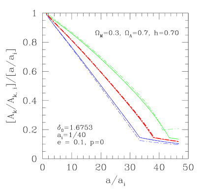
Figure 2: Comoving evolution of axis lengths in our ellipsoidal model. Solid lines are obtained by solving equation (6) numerically; dashed-dotted lines show equation (10).

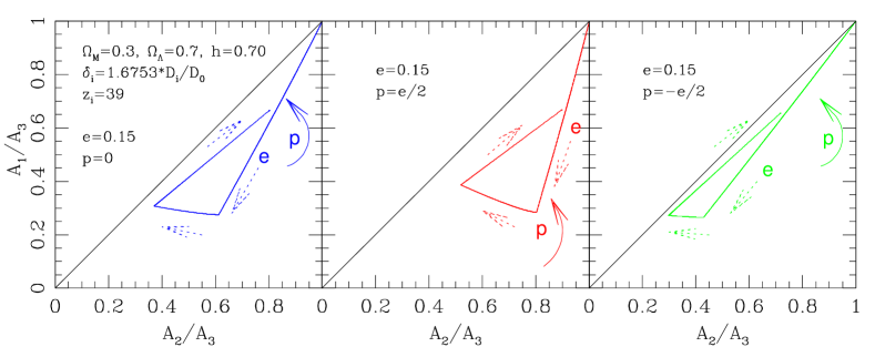
Figure 3: The ‘axis ratio plane’ for dark matter halos. Left, central and right panels show $p=0$ and $p=\pm~{}e/2$, respectively, when $e=0.15$. The initial redshift is $z_{\rm i}=39$, for an initially spherical patch with overdensity $\delta(t_{\rm i})=[D(t_{\rm i})/D(t_{\rm 0})]\delta(t_{0})$, where $\delta(t_{0})=1.6753$. See the main text for more details.

2.2 An analytic approximation

To characterize the dynamics of a collapsing object, one must solve numerically the coupled partial differential equations for the ellipsoidal collapse, as shown in Figure 1. However, there is a useful analytic approximation to the exact solution which provides considerable insight. By extending results in White & Silk (1979), Shen et al. (2006) show that

$${A_{\rm k}(t)\over A_{\rm k}(t_{\rm i})}\,\frac{a(t_{\rm i})}{a(t)} \simeq 1-\frac{D(t)}{D(t_{\rm i})}\lambda_{\rm k}(t_{\rm i})$$ (10)

$$-{A_{\rm h}(t_{\rm i})\over A_{\rm k}(t_{\rm i})}\Big{[}1-\frac{D(t)}{D(t_{\rm i})}{\delta(t_{\rm i})\over 3}-\frac{a_{\rm e}(t)}{a(t)}\Big{]},$$

where $A_{\rm h}(t_{\rm i})=3/\sum_{\rm j}A_{\rm j}^{-1}(t_{\rm i})$ and $a_{\rm e}(t)$ is the expansion factor of a universe with initial density contrast $\delta(t_{\rm i})\equiv\sum_{\rm j}\lambda_{\rm j}(t_{\rm i})$. This approximation to the full ellipsoidal collapse model can be thought of as correcting the Zeldovich (1970) approximation by the factor by which it is wrong for a sphere (Lam & Sheth 2008).

To first order in $\delta(t_{\rm i})$,

$$\frac{A_{1,3}(t)}{A_{1,3}(t_{\rm i})}\frac{a(t_{\rm i})}{a(t)}\simeq\frac{a_{\rm e}(t)}{a(t)}-\frac{\delta(t_{\rm i})}{3}(p\pm 3e)\Big{[}1+{D(t)\over D(t_{\rm i})}-{a_{\rm e}(t)\over a(t)}\Big{]}$$ (11)

$$\frac{A_{2}(t)}{A_{2}(t_{\rm i})}\frac{a(t_{\rm i})}{a(t)}\simeq\frac{a_{\rm e}(t)}{a(t)}+\frac{\delta(t_{\rm i})}{3}2p\,\Big{[}1+{D(t)\over D(t_{\rm i})}-\frac{a_{\rm e}(t)}{a(t)}\Big{]}.$$ (12)

Notice that when $p=0$, then

$$\frac{A_{2}(t)}{A_{2}(t_{\rm i})}\simeq\frac{a_{\rm e}(t)}{a(t_{\rm i})};$$ (13)

in this case, the second axis evolves exactly as in the spherical model, since for the spherical case $e\equiv p=0$, $\lambda_{\rm k}(t_{\rm i})\equiv\lambda(t_{\rm i})\equiv\delta(t_{\rm i})/3$ and so $A_{\rm k}(t)\equiv A(t)\rightarrow A(t_{i})[a_{e}(t)/a(t_{i})]$. In general, the second axis evolves very similarly to that for a spherical model with the same initial overdensity $\delta(t_{\rm i})$. In this respect, a spherical collapse can be roughly seen as an ‘imperfect’ ellipsoidal model, where the virialization is identified with the collapse of the second axis.

Figure 2 shows how well the approximation works in the LCDM model assumed in this study. Solid lines show numerical solutions of equation (6) in comoving units; dashed-dotted lines show the analytic approximation (equation 10). As evident from the figure, the approximation is rather good until the collapse of the third axis, as expected.

2.3 The axis ratio plane: dark halo evolution

The evolution of triaxial objects can be conveniently described by a two-dimensional ‘axis ratio plane’, showing the shortest-to-longest ($A_{1}/A_{3}$) versus intermediate-to-longest ($A_{2}/A_{3}$) axis ratios. Figure 3 shows what our ellipsoidal collapse model predicts for a few different combinations of prolateness and ellipticity, as indicated in the panels, when $\delta(t_{\rm i})=[D(t_{\rm i})/D(t_{\rm 0})]\delta(t_{0})$ and $z_{\rm i}=39$. Note that $\delta(t_{0})=1.6753$ is again the usual spherical collapse linear value in the concordance cosmology, at the present time.

The axis ratio plane provides useful insights into the evolution of dark matter halos. The trajectory of a collapsing object in the plane is as follows: down and to the left, as the shortest axis shrinks more rapidly than the other two (first line); then further to the left and slightly upwards, after the shortest axis has frozen out, while the second axis continues to shrink faster than the longest axis (second line); finally upwards and to the right, after the second axis has also frozen out, so only the longest is shrinking (third line), until the third axis also freezes out, at which point the object is defined as being virialized.

The slope of the first line is steeper when $p=e/2$, shallower when $p=-e/2$. The evolution proceeds further down the plane as $e$ increases, at fixed $p$, and is confined in the region between the bisector of the plane and the line characterized by $p=e/2$. Hence, when $p=e/2$ and $e>0$, the object is more likely to form a pancake (i.e. lower right region of the plane), while when $p=-e/2$ a filament is more likely to occur (i.e. lower left region). Also, for small values of ellipticity, the final shape does not depart significantly from the spherical case (upper right region of the plane).

The fact that $p$ determines the slope of the initial motion in the plane, whereas $e$ controls how far the initial collapse progresses, can be understood as follows. Initially, i.e., when $\lambda_{1}\ll 1$,

$$\frac{A_{1}}{A_{3}}=\frac{1-\lambda_{1}}{1-\lambda_{3}}\simeq 1-2\delta(t_{\rm i})e,$$ (14)

$$\frac{A_{2}}{A_{3}}=\frac{1-\lambda_{2}}{1-\lambda_{3}}\simeq\frac{A_{1}}{A_{3}}+\delta(t_{\rm i})(e+p).$$ (15)

Therefore, for a given $\delta(t_{\rm i})$, the ratio $A_{1}/A_{3}$ is a function of $e$ only: if $e$ increases then $A_{1}/A_{3}$ decreases, and at fixed $A_{1}/A_{3}$ (or, equivalently, for a given $e$) the prolateness $p$ increases as $A_{2}/A_{3}$ increases. This effect is indicated in Figure 3 by the circular arrows.

To next order in $\delta(t_{\rm i})$

$$\frac{A_{1}(t)}{A_{3}(t)} \simeq \frac{A_{2}(t)}{A_{3}(t)}\frac{1-\delta(t_{\rm i})(1+3e+p)/3}{1-\delta(t_{\rm i})(1-2p)/3}\times$$ (16)

$$\Big{\{}1-{\delta(t_{\rm i})\over 3}{a(t)\over a_{\rm e}(t)}(3e+p)\Big{[}1+{D(t)\over D(t_{\rm i})}-{a_{\rm e}(t)\over a(t)}\Big{]}\Big{\}}\over\Big{\{}1+{2\delta(t_{\rm i})\over 3}{a(t)\over a_{\rm e}(t)}p\Big{[}1+{D(t)\over D(t_{\rm i})}-{a_{\rm e}(t)\over a(t)}\Big{]}\Big{\}}.$$

In particular, when $p=0$:

$$\frac{A_{1}(t)}{A_{3}(t)}\simeq(1+3e)\Big{\{}1+\delta(t_{\rm i})e\Big{[}1-\Big{(}1+{D(t)\over D(t_{\rm i})}\Big{)}{a(t)\over a_{\rm e}(t)}\Big{]}\Big{\}}{A_{2}(t)\over A_{3}(t)}.$$ (17)

Motivated by this, we have parametrized the evolution in this plane as follows. If $f(e)$ denotes the distance along the first line, then, for a given $p$,

$$f(e)=\sqrt{(1-A_{2}/A_{3})^{2}+(1-A_{1}/A_{3})^{2}},$$ (18)

and

$$\frac{A_{1}}{A_{3}}-k(p)\frac{A_{2}}{A_{3}}=b.$$ (19)

The constraint that $A_{1}/A_{3}=1$ when $A_{2}/A_{3}=1$ implies that $b=1-k(p)$, and therefore:

$$f(e)=\Big{(}1-\frac{A_{2}}{A_{3}}\Big{)}\sqrt{1+k^{2}(p)}.$$ (20)

We found $k(p)=1.858$ when $p=0$, $k(p)=3.803$ when $p=e/2$, and $k(p)=1.253$ when $p=-e/2$ for the collapse of the shortest axis. For the turnaround of the second line, parametrized in the same fashion, $k(p)=1.084$ when $p=0$, $k(p)=1.253$ when $p=e/2$ and $k(p)=1.034$ at $p=-e/2$. The slope of the final part of the evolution (third line), when $A_{2}$ and $A_{1}$ are both frozen, is simply given by $A_{1}(t_{\rm f})/A_{2}(t_{\rm f})$. Hence, it approaches unity (i.e. parallel to the bisector of the plane) when $A_{1}/A_{3}\simeq A_{2}/A_{3}$, and it is always lesser than unity otherwise, since $A_{1}(t_{\rm f})\leq A_{2}(t_{\rm f})$.

3 Initial and evolved halo shapes

The discussion above shows how the initial values of $\delta,e,p$ determine the future evolution of the object, including its shape. Our next task is to determine how the initial distribution of $e$ and $p$ values depends on halo mass. We use the algorithm of Sheth & Tormen (2002) to do this. Briefly, this requires the generation of the joint distribution of $\delta,e,p$ as a function of smoothing scale $R_{\rm i}$, finding the largest scale at which $\delta\geq\delta_{\rm ec}(e,p)$, and then associating the values $(\delta_{\rm ec},e,p)$ to the patch from which a halo of mass $M=\bar{\rho}\,4\pi R_{\rm i}^{3}/3$ formed. Since this algorithm has been used by other authors since (Sandvik et al. 2007), we do not provide details here, but refer the reader to Appendix B in Sheth & Tormen (2002), and to Bond et al. (1991), Bower (1991) and Lacey & Cole (1993) for further details.

3.1 Mass-dependent shapes from scale-dependent initial conditions

Figure 4 illustrates how our model for halo shapes works. The top left panel shows the distribution of initial axis ratios for small patches ($M=10^{13}h^{-1}M_{\odot}$) which the ellipsoidal collapse model predicts are destined to become low mass halos at the present time. The bottom left panel shows the distribution of final axis ratios at virialization (see Section 2). The panels on the right show the analogous quantities for more massive halos ($M=10^{14}h^{-1}M_{\odot}$).

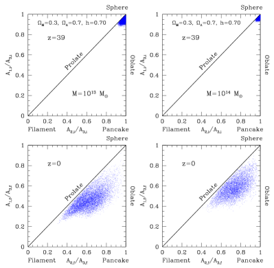
Figure 4: Distribution of initial (top panels) and final (bottom panels) axis ratios in our model, for halos of mass $M=10^{13}h^{-1}M_{\odot}$ (left) and $10^{14}h^{-1}M_{\odot}$ (right). Initial conditions are specified by combining the statistics of Gaussian random fields with the ellipsoidal collapse model, following Sheth & Tormen (2002).

The plot shows that halos are, in general, predicted to be triaxial, with a slight tendency to be more prolate than oblate. In addition, massive halos are predicted to be more spherical than less massive halos, both initially and finally. This is primarily a consequence of the fact that the larger patches from which massive halos form have, on average, smaller values of ($e,p$). The trend is consistent with the findings of Bernardeau (1994), who argued that in perturbation theory larger halos are expected to be rounder.

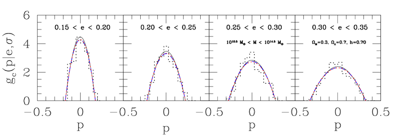
Figure 5: Distribution of prolateness at fixed halo mass and ellipticity, $g_{c}(p|e,\sigma)$, in our model (dotted histograms). Theoretical curves (solid lines) are from equation (22) with different values of $e$, as specified in each panel. The initial distribution $g(p|e,\sigma,\delta)$ is also shown, with long-dashed lines (i.e. equation 23), as well as its approximation (i.e. dotted lines). See the main text for more details.

3.2 The conditional prolateness distribution

The joint distribution of $\lambda_{1}\geq\lambda_{2}\geq\lambda_{3}$ was derived by Doroshkevich (1970) for Gaussian random fields (see Lam, Sheth & Desjacques 2009 for an extension to non-Gaussian fields that are of the ‘local’ type). The equivalent expression, in terms of e, p and $\delta$, is:

$$g(e,p,\delta|\sigma)=p(\delta|\sigma)\,g(e,p|\delta,\sigma){}$$ (21)

$$= {}\frac{e^{-\frac{\delta^{2}}{2\sigma^{2}}}}{\sigma\sqrt{2\pi}}\frac{1125}{\sqrt{10\pi}}e(e^{2}-p^{2})\Big{(}\frac{\delta}{\sigma}\Big{)}^{5}e^{-\frac{5}{2}\frac{\delta^{2}}{\sigma^{2}}(3e^{2}+p^{2})}.$$

Doroshkevich’s formula is the product of two independent distributions, a Gaussian for $\delta/\sigma$, and one which is a combination of the other five independent elements of the deformation tensor of which the $\lambda_{\rm j}$ are the eigenvalues (Sheth & Tormen 2002). Integration of equation (21) over $\delta$ yields the joint distribution of ellipticity and prolateness, $g(e,p|\sigma)$. A further integration over $p$ gives the distribution of ellipticities as a function of halo mass ($\sigma$), $f(e|\sigma)$. This integral can be computed analytically (c.f. equation 24 of Lam et al. 2009).

For a given ellipticity, we can predict the distribution of $p$’s that will produce collapsed objects at any given redshift (say, $z=0$). In detail, for $\delta_{\rm ec}(e,p)$ as in equation (9), we define $\Theta(\delta,e,p)=1$ if $\delta\geq\delta_{ec}(e,p)$ and $\Theta(\delta,e,p)=0$ otherwise. Then we impose the requirement that the perturbation had collapsed (at $z=0$) by computing

$$g_{\rm c}(p|e,\sigma)=\frac{g_{\rm c}(e,p|\sigma)}{\int_{-e}^{e}{\rm d}p~{}g_{\rm c}(e,p|\sigma)}{}$$ (22)

$$= {}\frac{\int_{0}^{\infty}{\rm d}\delta\,g(e,p|\delta,\sigma)\,p(\delta|\sigma)\ \Theta[\delta\geq\delta_{\rm ec}(e,p)]}{\int_{\rm-e}^{\rm e}{\rm d}p\int_{0}^{\infty}{\rm d}\delta\,g(e,p|\delta,\sigma)\,p(\delta|\sigma)\,\Theta[\delta\geq\delta_{\rm ec}(e,p)]}.$$

Plots of equation (22) are shown in Figure 5 with solid lines. We can further quantify if the difference between $g(p|e,\delta,\sigma)$ and $g_{\rm c}(p|e,\sigma)$ is relevant (i.e. dependence of barrier and epoch) by computing:

$$g(p|e,\delta,\sigma)=\frac{g(e,p|\delta,\sigma)}{\int_{-e}^{e}{\rm d}p~{}g(e,p|\delta,\sigma)}{}$$ (23)

$$= {}{25y^{3}\,(1-p^{2}/e^{2})\,{\rm e}^{(5y^{2}/2)(1-p^{2}/e^{2})}/e\over\sqrt{10\pi}(5y^{2}-1)\,{\rm e}^{(5y^{2}/2)}{\rm erf}(\sqrt{5y^{2}/2})+10y}.$$

where $y=e\delta/\sigma$. Long-dashed lines in Figure 5 show this distribution: as evident from the panels, the difference between (22) and (23) is negligible. In fact, if one ignores the exponential prefactor in equation (21), then it is straightforward to show that

$$g(p|e,\delta,\sigma)\simeq g(p|e)=(3/4)(1-p^{2}/e^{2})/e.$$ (24)

Dotted curves in Figure 5 show that this is a very good approximation.

3.3 Universal conditional axis ratio distributions at late times

In equation (22), the mass and epoch dependencies actually cancel out, i.e. $g_{\rm c}(p|e,\sigma)\equiv g_{\rm c}(p|e)$. This suggests that nonlinear evolution will not change the conditional distribution $g_{\rm c}(p|e,\sigma)$ from that which is set by the initial conditions. To see why, recall that the axis ratio $A_{1}/A_{3}$ is specified once $\delta(t{\rm{}_{i}})$ and the ellipticity are fixed (c.f. equation 14). Moreover, if $\delta(t{\rm{}_{i}})$ and $e$ are fixed, then $A_{1}/A_{2}=(A_{1}/A_{3})/(A_{2}/A_{3})$ is only a function of the prolateness (c.f. equation 15). Hence, for a fixed mass, equation (22) can be equally expressed in terms of ($e,p$), or as a function of ($A_{1}/A_{2},A_{1}/A_{3}$). I.e., if we define $A_{12}\equiv A_{1}/A_{2}$ and $A_{13}\equiv A_{1}/A_{3}$, then

$$p(A_{12}|A_{13},\delta,\sigma) = \frac{g(A_{12},A_{13}|\delta,\sigma)}{p(A_{13}|\delta,\sigma)}$$ (25)

$$= \frac{3}{2(1-A_{13})}\,\Big{[}1-\frac{(2A_{12}-1-A_{13})^{2}}{(1-A_{13})^{2}}\Big{]}$$

$$\times \exp\Big{\{}-{5\over 8\sigma^{2}}(2A_{12}-1-A_{13})^{2}\Big{\}},$$

where the final expression follows from setting

$$g(A_{12},A_{13}|\delta,\sigma)\,{\rm d}A_{12}\,{\rm d}A_{13}=g(e,p|\delta,\sigma)\,{\rm d}e\,{\rm d}p.$$ (26)

At small masses, the exponential term $\to 1$, making this distribution almost universal, i.e. independent of mass and epoch. This remarkable feature will guide the interpretation of our results on halo shapes in the next section.

4 Comparison with high resolution simulations

The previous section showed how we combine the nonlinear ellipsoidal model for halo collapse and virialization (Section 2) with the excursion set theory (Section 3), to model the initial and evolved shape distributions of dark matter halos. Here, we investigate to what extent our simple analytic prescription is able to reproduce results from $N$-body simulations of Jing & Suto (2002).

For their statistical analysis of halo shapes, Jing & Suto (2002) identified halos at $z=0,0.5,1$ in simulations of a cosmology with ($\Omega_{\rm M}=0.3,\Omega_{\rm\Lambda}=0.7,h=0.7$). The simulations used $N=512^{3}$ particles in a 100 h^-1Mpc box. Halos were identified using a friends-of-friends (FOF) algorithm with link-length $b=0.1d$, where $d$ is the interparticle separation. Each of their FOF halos contains more than $10^{4}$ particles. The lower mass limit of their halo catalog is $6.2\times 10^{12}h^{-1}M_{\odot}$. They provided a set of fitting formulae which allow simple tests of our triaxial model: in particular the mass and redshift dependence of the axis ratios, and the probability distribution functions of the axis ratios.

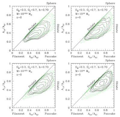
Figure 6: Distribution of final axis ratios in our model for halos of different masses (solid contours), as specified in the panels. Each halo has been evolved using the ellipsoidal collapse model. The generic evolution is initially towards an oblate, pancake-like structure, followed by a shift towards a more prolate shape, as the other axes also begin to shrink. Dotted lines are the joint distribution which Jing & Suto (2002) report describe the halos in their simulations, in the concordance cosmology ($\Omega_{\rm M}=0.3,\Omega_{\rm\Lambda}=0.7,h=0.7$).

4.1 Joint distribution of axis ratios

By averaging over the correct, mass dependent, distribution of initial shape parameters, each evolved through the ellipsoidal collapse model, we are also able to make predictions for how the distribution of final shapes depends on halo mass. The solid contours in Figure 6 show the joint distribution of ($A_{2}/A_{3},A_{1}/A_{3}$) we predict; contours show levels where the probability has fallen to $1/2,1/4,1/8,1/16$ of the maximum value. The dotted lines represent the joint distribution which Jing & Suto (2002) report describe the halos in their simulations. Note, for the moment, that our model appears to be in reasonable agreement with the simulations only around $M\simeq 10^{\rm 13}h^{-1}M_{\odot}\simeq M_{*}$ . While this agreement is gratifying, the fact that the mismatch is mass-dependent is potentially troubling. Jing & Suto find that the low mass halos are actually slightly more spherical than massive halos. Although the effect is weak, it has since been confirmed by a long list of authors (see Section 1). In contrast, in our model, it is the massive halos which are expected to be more spherical (Figure 4). The trend we find is consistent with perturbation theory (Bernardeau 1994; Pogosyan et al. 1998; see Park et al. 2007, Dalal et al. 2008 and Park, Kim & Park 2010 for more recent discussion of this point).

To show this more clearly, Figure 7 compares the final distribution of $A_{1}/A_{3}$ in our model (dotted) with the distribution in Jing & Suto’s simulations (solid) at $z=0$. Again, note that the agreement is reasonable around $M_{*}$, but that the predicted distribution is broader than the simulations at low and high masses. Note also that the left panels in the figure show our results without any arbitrary rescaling, while in the right panels we apply the empirical rescaling they suggest, which effectively removes the trend with mass.

Park, Kim & Park (2010) have argued that the main reason for this discrepancy may be due to the halo definition itself, and to the halo environment. They used a more sophisticated halo finding algorithm (from Kim & Park 2006) which identifies gravitationally self-bound and tidally stable halos. They showed that the dependence of $A_{1}/A_{3}$ on local density is stronger for more massive isolated halos, and argued that tidal interactions between neighboring halos make them more spherical on average. In particular, Park, Kim & Park (2010) pointed out that the main problem relies primarily on the FOF halo finder. This is because the FOF identification scheme cannot distinguish between objects connected by filaments. For example, if two massive and almost spherical neighboring halos are slightly connected by a filament, the FOF halo finder will consider those objects as one big structure, and erroneously assign a rather elongated shape to it. Therefore, the FOF scheme will find that more massive objects are more elongated, while in reality this is an artifact of the FOF procedure. Park et al. (2010) went one step further; after running their halo finder algorithm, they identified subhalos within FOF halos, and classified their FOF halos into central (i.e. the most massive halos in each group of halos and subhalos), satellite (i.e. halos which are not the central ones in each group of halos and subhalos), and isolated halos (i.e. structures which do not overlap with other halos, but which can have close neighbor halos and subhalos). After this classification, they found that the degree of halo sphericity increases with mass (i.e. more massive objects are rounder) for isolated halos, up to about $2\times 10^{14}h^{-1}M_{\odot}$ – a similar trend we find in our theoretical study.

Figure 7: Distribution of the minor-to-major axis ratio, $A_{1}/A_{3}$, in our model (dotted) and in Jing & Suto’s (2002) numerical simulations (solid). Raw data are plotted in the left panels, while in the right panels data are rescaled according to their prescription.

4.2 Conditional axis-ratio distributions

The left panel of Figure 8 compares the conditional minor-to-intermediate axis distribution of $A_{1}/A_{2}$ for a given range of $A_{1}/A_{3}$ in our model (histograms), with Jing & Suto’s simulations (solid lines) at $z=0$. In this case, instead, we find remarkably good agreement with the numerical measurements.

Recall that we had argued that the conditional prolateness distribution $g(p|e,\delta,\sigma)$ in the initial conditions (equation 25 and Figure 5), depends only weakly on $\delta/\sigma$, so we expect the conditional minor-to-intermediate axis ratio distribution of the evolved object, $p(A_{12}|A_{13},\delta,\sigma)$, to be similarly universal – independent of mass and time; whether this equivalence is due to statistics, rather than physics, is subject of ongoing work. The agreement with Jing & Suto’s simulations suggests that $p(A_{12}|A_{13},\delta,\sigma)$ is indeed preserved from the initial conditions. In fact, except for the exponential factor in our equation (25), our theoretically motivated expression for this distribution is exactly the same as that of Jing & Suto’s empirical fitting formula.

More recently, Wang et al. (2010) have also found that, in their simulations, $p(A_{12}|A_{13})$ is independent of mass and epoch. They also noted that the final redshift dependence of the short-to-intermediate axial ratio is much weaker than the other two ratios, indicating that new material tends to be accreted along the major axes of halos. Our formula (25) provides the theoretical/physical explanation for their findings.

In this context, we note that Lee, Jing & Suto (2005) also presented an analytic expression for the axis ratio distribution of triaxial objects, and claimed that it successfully reproduces the conditional intermediate-to-major axis ratio distribution. However, in their Figure 5 which is supposed to support this claim, it is the minor-to-intermediate distribution from the numerical simulations, $p(A_{1}/A_{2}|A_{1}/A_{3})$, which is compared with their theory curve for the intermediate-to-major axis ratio distribution, $p(A_{2}/A_{3}|A_{1}/A_{3})$. While this invalidates their claim (see also Appendix A for more discussion on the flaw in their model), it does raise the question of why the formula for one distribution happened to describe another?

Our model shows why. When $\lambda_{1}\ll 1$, then $A_{1}/A_{2}\simeq 1-\delta(t_{\rm i})(e+p)$, while $A_{2}/A_{3}\simeq 1-\delta(t_{\rm i})(e-p)$. However, the sign difference in the prolateness does not alter the Jacobian of the two different transformations: ($e,p\rightarrow A_{2}/A_{3},A_{1}/A_{3}$) and ($e,p\rightarrow A_{1}/A_{2},A_{1}/A_{3}$). Hence, $p(A_{2}/A_{3}|A_{1}/A_{3})\,{\rm d}(A_{2}/A_{3})\equiv p(A_{1}/A_{2}|A_{1}/A_{3})\,{\rm d}(A_{1}/A_{2})$, and therefore

$$p(A_{2}/A_{3}|A_{1}/A_{3})={(A_{1}/A_{2})\over(A_{2}/A_{3})}\cdot p(A_{1}/A_{2}|A_{1}/A_{3}).$$ (27)

Thus, at fixed $A_{1}/A_{3}$, the minor-to-intermediate or the intermediate-to-major axis ratios distributions are both equivalent, and so ‘universal’. Although equivalent, clearly these distributions are indeed different and neatly distinguishable: the right panel of Figure 8 compares now the conditional intermediate-to-major axis distribution of $A_{2}/A_{3}$ for a given range of $A_{1}/A_{3}$ in our model (histograms), with Jing & Suto’s simulations (solid lines) at $z=0$. As evident from the plots, $p(A_{2}/A_{3}|A_{1}/A_{3})$ is more asymmetric than $p(A_{1}/A_{2}|A_{1}/A_{3})$, and the difference is more significant for lower values of $A_{1}/A_{3}$.

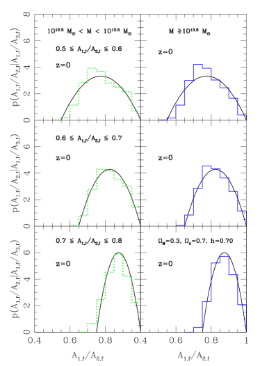
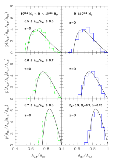
Figure 8: Conditional distributions ($A_{1}/A_{2}|A_{1}/A_{3}$) – left panel – or ($A_{2}/A_{3}|A_{1}/A_{3}$) – right panel – in our model (histograms), and in the numerical simulations of Jing & Suto (2002) (solid lines). Results are shown for two different mass ranges (both at $z=0$) and for different values of $A_{1}/A_{3}$, as labeled.

4.3 Caveats

In general, a direct comparison between our theoretical model and $N$-body simulations is both challenging and subtle. This is primarily because there is still no unanimous agreement about how to define a gravitationally bound object; i.e the very definition of what a non-spherical dark matter halo is, both in simulations and observationally, is a non-trivial problem. Determining which material belongs to a halo and what lies beyond is an open problem (Prada et al. 2006; Bett et al. 2007; Diemand, Kuhlen & Madau 2007; Cuesta et al. 2008). Common methods for defining virialized halos in simulations include: spherical overdensity, tree algorithms based on the branches of the halo merger trees, two-step procedures with post-processing, maximum circular velocity, etc., (see Klypin et al. 2010, and references therein for more discussion). Clearly, the distribution of halo shapes measured from simulations depends critically on the halo definition. For instance, Bett et al. (2007) found that spherical overdensity halos are more spherical than FOF or TREE halos, and that FOF halos show a much broader distribution of shapes and a strong preference for prolateness. This fact complicates the comparison and interpretation of theory against any numerical study.

Since we are most interested in halo shapes, measurements which do not perform spherical averages are more closely related to our models. Jing & Suto (2002) used one such method: a friend-of-friend algorithm (Davis et al. 1985; Lacey & Cole 1994). This is a percolation scheme that links together all particles that are closer than $b=0.2d$, where $d$ is the mean interparticle separation. This value of $b$ returns objects which are approximately 200 times the background density: it makes no assumptions about the shape of the resulting object. However, it may group distinct halos together into the same object, confusing the comparison with theory (White 2001; Tinker et al. 2008; Lukic et al. 2009). This problem is more serious for halos in higher density regions; since high density regions have top-heavy mass functions (Sheth & Tormen 2002), massive halos identified by this algorithm may be erroneously considered to be elongated.

Jing & Suto (2002) used $b=0.1d$, so their FOF clumps are smaller and denser than those defined using the more conventional $0.2d$. As a result, they are less likely to suffer from spuriously linked halos. However, in effect, their procedure identifies only the central parts of the more conventional halo.

As a further complication, having settled on a halo definition, some authors only study shapes of a subset of the halo population. E.g., Jing & Suto (2002), only analyzed halos which looked ‘relaxed’: at fixed mass, this is almost certainly a more homogeneous subset of the entire population. Our model does not account for this additional selection.

Despite such difficulties in the model/simulation comparison, we believe such an exercise is still useful, because there are other reasons why we anticipate disagreement between model and simulations. E.g., the ellipsoidal collapse itself is a significant oversimplification of the more complex nonlinear gravitational evolution – it cannot be expected to fully capture the dynamics of $N$-body simulations. Despite all these caveats, we believe the remarkably good agreement between the measured conditional axis ratio distributions and our equation (25) (Figure 8) is non-trivial.

5 Discussion

We presented a model to describe the shape distribution of bound objects based on Rossi (2008), which is a simple extension of that introduced by Bond & Myers (1996) and used by Sheth, Mo & Tormen (2001) to estimate the abundance by mass of these objects. Our analytic prescription is made of two independent parts: one is a scheme for how an initially spherical patch evolves and virializes, for which we adopted the ellipsoidal collapse dynamics (Section 2, Figure 1); the other is the correct assignment of initial shapes to halos of different masses, achieved through the excursion set formalism (Section 3, Figure 4). Along the way, we discussed an analytic approximation to the evolution, considerably more rigorous than the Zeldovich approximation (Section 2.2, Figure 2). And we introduced a useful planar representation of halo axis ratios, which gives a simple intuitive framework for discussing the dynamics of collapsing regions (Section 2.3, Figure 3).

We showed that the model is able to provide a reasonable description of the minor-to-major axis ratio distribution seen by Jing & Suto (2002) in their numerical simulations only within a limited mass range (i.e. around $M\simeq 10^{\rm 13}h^{-1}M_{\odot}\simeq M_{*}$). Outside this range, Jing & Suto found that low-mass halos are preferentially more spherical than high-mass halos, whereas in our model, the high-mass halos are more spherical (Figures 6 and 7). We argued that some the disagreements may originate from differences in halo types and mass range, and may be alleviated if we consider only isolated halos. This is because Park, Kim & Park (2010) find that, on average, high-mass isolated halos are indeed more spherical than low-mass ones, and the difference is larger in high density/shear regions (see their Section 3.4 and their Figures 9, 10 and 11, for details on how to select isolated clusters from simulations). Note also that isolated clusters can be readily identified from an observational catalog, as done for example in Park & Hwang (2009) for a sample of Abell galaxy clusters (their Section 2.2 gives a detailed explanation on how the selection is performed). The finding of Park, Kim & Park (2010) has an interesting connection to recent observational work on mass scales where the hypothesis that a halo hosts only one galaxy may be appropriate. For early-type galaxies in the SDSS, although the observed projected axis ratio $b/a$ increases with increasing stellar mass or luminosity, it decreases at the highest masses (Bernardi et al. 2008, 2010). This reversal is thought to arise because the most massive galaxies tend to be in regions (e.g., at cluster centers) where recent radial mergers may have made them prolate. Fasano et al. (2010) come to a similar conclusion based on an analysis of the intrinsic shape distribution of BCGs from the WINGS survey (Fasano et al. 2006; Varela et al. 2009). They propose that the prolateness of the BCGs (in particular the cDs) could reflect the shape of the associated dark matter halos (also see Smith et al. 2010). Hence, while it is tempting to conclude that the discrepancy between mass dependent trends in simulations and theory will be alleviated if we only consider isolated halos, we note that Jing & Suto (2002) eliminated halos in their simulations which were not relaxed. If these had suffered recent mergers, then they may already have removed the most prolate halos from their sample. Further investigation of this point is the subject of ongoing work.

Despite this disagreement about the distribution of minor-to-major axis ratio, we found very good agreement between our model and the conditional minor-to-intermediate axis ratio distribution measured from simulations (Figure 8). In particular, we showed that our model provides physical motivation for the empirical fitting formula obtained in Jing & Suto (2002) from numerical studies (our equation 25). In our model, this distribution is closely related to the conditional prolateness distribution in the initial conditions (Section 3.2, Figure 5). Unfortunately, results in Lam et al. (2009) suggest that this distribution is unlikely to be able to discriminate between Gaussian initial conditions and ones where the primordial non-Gaussianity is of the ‘local’ type (i.e. Rossi, Chingangbam & Park 2010).

We also discussed the agreement/disagreement between theory and numerical predictions, in the context of known problems and limitations in the modelling to difficulties in making shape measurements from simulations.

We are currently studying the following improvements and extensions to our model:

1. Our model makes the extremely simple assumption that axis lengths freeze-out once they have shrunk to a sufficiently small size. Subsequent violent relaxation effects associated with particles which collapse along other axes may change this size – something our current model does not consider. For instance, massive halos are expected to have assembled their mass more recently than low mass halos. Therefore, relaxation effects may have had more time to change the axis ratios of low mass halos than of higher mass halos. If the net effect of this relaxation is to make the halos more spherical than they would otherwise have been, then accounting for it may help resolve the discrepancy between our model and simulations. Note that halos having smaller amounts of substructures tend to be closer to virial equilibrium (e.g. Giocoli et al. 2010), but there has been no study of whether or not haloes with abnormally small sub-structure (for their mass) are rounder.

2. Testing different collapse criteria, and other prescriptions for the external tidal field (e.g., Angrick & Bartelmann 2010).

3. Accounting for correlations between the properties of halos and their environment (assembly bias), as seen in $N$-body simulations (Sheth & Tormen 2004; Ragone-Figueroa & Plionis 2007). Environmental effects can have a significant impact on the properties of virialized halos because, in the ellipsoidal model, the critical density threshold $\delta_{\rm ec}$ depends strongly on the initial values of $e$ and $p$, and these distributions depend on environment (Keselman & Nusser 2007; Wang, Mo & Jing 2007; Desjacques 2008). In our current implementation, only the initial density of the surrounding environment matters.

4. Accounting for correlations between formation times and halo shapes, as seen in $N$-body simulations (Ragone-Figueroa et al. 2010).

5. Modifying the algorithm of Sheth & Tormen (2002) to account for correlated steps, following Maggiore & Riotto (2010) and De Simone et al. (2010), when deriving our initial conditions.

6. Including the effects of baryonic physics. The condensation of baryons to the centers of dark matter halos is known to change their shape (Dubinski 1994; Holley-Bockelmann et al. 2002; Kazantzidis et al. 2004; Debattista et al. 2008).

7. Estimating correlations between halo shapes. This is possible because, in our model, the final shape is determined by the initial conditions, and correlations in the initial conditions can be quantified. Thus, in our model, correlations at the present time are obtained by taking the appropriate average over the initial correlations – this average being determined by the mapping from $(e,p)\rightarrow(A_{2}/A_{3},A_{1}/A_{3})$. Most published estimates of the correlation between shapes do not account for this mapping.

8. Describing the shapes of subhalos as well as voids (e.g., Shandarin et al. 2006; D’Aloisio & Furlanetto 2007; Platen et al. 2008).

We conclude with the observation that while numerical studies are indispensable for quantifying the shapes and structures of dark matter halos, we hope that our simple procedure may provide a complementary theoretical framework for understanding halo shapes, and how these shapes are correlated with larger-scale structures.

Appendix A Comparison with the model of Lee, Jing & Suto (2005)

The main text describes a number of inconsistencies in the work of Lee et al. (2005). Besides the mismatch between $p(A_{1}/A_{2}|A_{1}/A_{3})$ and $p(A_{2}/A_{3}|A_{1}/A_{3})$ (see Section 4.2), we also stated in the main text that their approach does not reduce to the Zeldovich approximation – despite the fact that they believe it does.

To see why, note that their equation (2) gives the usual expression for the nonlinear density in the Zeldovich approximation – the same one we use. Namely, if we use $R_{\rm i}$ to denote the initial length of axis $i$, and $r_{\rm i}$ its length at a later time, then their equation (2) comes from setting $r_{\rm i}/R_{\rm i}=1-D(t)\lambda_{\rm i},$ where $\lambda_{i}$ is the eigenvalue of the initial shear tensor. Note that there is no square root factor in the relation between $\lambda_{\rm i}$ and the Zeldovich-evolved axis length $r_{\rm i}/R_{\rm i}$.

Lee et al. (2005) then define ($a,b,c$) to be the eigenvalues of the inertia tensor. For a homogeneous ellipsoid with axis ratios ($A,B,C$), the inertia tensor eigenvalues ($a,b,c$) are related to ($A^{2}$, $B^{2}$, $C^{2}$), whereas their equation (7) sets $a$ equal to the square root of $A$. I.e., they have put the square root on the wrong side of the equation. Therefore, their expressions will not reduce correctly to the Zeldovich approximation at early times.

Note that their equation (8) does in fact have the correct relation between the semi-axis lengths and eigenvalues (because it has been taken correctly from Equation 7.2 of Bardeen et al. 1986). In this notation, $\zeta_{1}=a^{2}$ where the $\zeta_{i}$ are the eigenvalues of the inertia tensor, but Lee et al. (2005) incorrectly call ($a,b,c$) the eigenvalues of inertial tensor, when they are in fact the semi-axis lengths (see text above Equation 7.2 of Bardeen et al. 1986). However, by equation (15), Lee et al. are referring to $b/c$ as ratios of axis lengths, rather than as ratios of eigenvalues. Their sloppiness about the important difference between these two gives rise to the following problem. If ($a,b,c$) are axis lengths, then the square root factor in their equation (7) means they will not recover the Zeldovich approximation, which does not have a square root factor. If they are eigenvalues of the inertia tensor, then they have put the square root in the wrong place, so again, they will not recover the Zeldovich approximation.

Unfortunately, Jing & Suto (2002) are also ambiguous about just what it is they measured. Their equation (5) shows ($a,b,c$) as being axis ratios, whereas their text describes them as being obtained from diagonalizing the inertia tensor, hence eigenvalues (unfortunately, they don’t say explicitly which is the square-root of the other).

In a subsequent study on cosmic voids, Lavaux & Wandelt (2010) used some erroneous definitions from Lee et al. (2005) but still found excellent agreement between their analytic framework and measurements from numerical simulations. This is because they where “consistently wrong”, in that their derived quantities measured from the simulations suffer from the same flaw present in their theory. Hence, although their ellipticity definitions are incorrect, the comparison theory/simulations is still fair. We also note that the philosophy of our approach in modelling halo shapes is similar to theirs, although the details are different (see their Appendix B) and they matter (i.e. in particular the use of the ellipsoidal collapse barrier as in Equation 22, which allows one to distinguish between peaks and random positions). We will expand more on this important issue in a forthcoming publication.

References

- Albrecht et al. (2006) Albrecht, A., et al. 2006, arXiv:astro-ph/0609591
- Allgood et al. (2006) Allgood, B., Flores, R. A., Primack, J. R., Kravtsov, A. V., Wechsler, R. H., Faltenbacher, A., & Bullock, J. S. 2006, MNRAS, 367, 1781
- Angrick & Bartelmann (2010) Angrick, C., & Bartelmann, M. 2010, AA, 518, A38
- Araya-Melo et al. (2009) Araya-Melo, P. A., Reisenegger, A., Meza, A., van de Weygaert, R., Dünner, R.,& Quintana, H. 2009, MNRAS, 399, 97
- Audit et al. (1997) Audit, E., Teyssier, R., & Alimi, J.-M. 1997, AA, 325, 439
- Audit & Alimi (1996) Audit, E., & Alimi, J.-M. 1996, AA, 315, 11
- Banerjee & Jog (2008) Banerjee, A., & Jog, C. J. 2008, ApJ, 685, 254
- Bardeen et al. (1986) Bardeen, J. M., Bond, J. R., Kaiser, N., & Szalay, A. S. 1986, ApJ, 304, 15
- Barnes & Efstathiou (1987) Barnes, J., & Efstathiou, G. 1987, ApJ, 319, 575
- Barrow & Silk (1981) Barrow, J. D., & Silk, J. 1981, ApJ, 250, 432
- Bartelmann (1995) Bartelmann, M. 1995, AA, 303, 643
- Bartelmann & Schneider (2001) Bartelmann, M., & Schneider, P. 2001, Phys. Rep., 340, 291
- Bernardeau (1994) Bernardeau, F. 1994, ApJ, 427, 51
- Bernardi et al. (2010) Bernardi, M., Roche, N., Shankar, F., & Sheth, R. K. 2010, arXiv:1005.3770
- Bernardi et al. (2008) Bernardi, M., Hyde, J. B., Fritz, A., Sheth, R. K., Gebhardt, K., & Nichol, R. C. 2008, MNRAS, 391, 1191
- Bernstein (2010) Bernstein, G. M. 2010, MNRAS, 406, 2793
- Bernstein (2007) Bernstein, G. 2007, Statistical Challenges in Modern Astronomy IV, 371, 59
- Bernstein & Nakajima (2009) Bernstein, G. M., & Nakajima, R. 2009, ApJ, 693, 1508
- Bertschinger & Jain (1994) Bertschinger, E., & Jain, B. 1994, ApJ, 431, 486
- Bett et al. (2007) Bett, P., Eke, V., Frenk, C. S., Jenkins, A., Helly, J., & Navarro, J. 2007, MNRAS, 376, 215
- Bond & Myers (1996) Bond, J. R., & Myers, S. T. 1996, ApJS, 103, 1
- Bond et al. (1991) Bond, J. R., Cole, S., Efstathiou, G., & Kaiser, N. 1991, ApJ, 379, 440
- Bower (1991) Bower, R. G. 1991, MNRAS, 248,332
- Boylan-Kolchin et al. (2009) Boylan-Kolchin, M., Springel, V., White, S. D. M., Jenkins, A., & Lemson, G. 2009, MNRAS, 398, 1150
- Bradač et al. (2006) Bradač, M., et al. 2006, ApJ, 652, 937
- Bridle et al. (2009) Bridle, S., et al. 2009, Annals of Applied Statistics, 3, 6
- Broadhurst et al. (2008) Broadhurst, T., Umetsu, K., Medezinski, E., Oguri, M., & Rephaeli, Y. 2008, ApJ, 685, L9
- Carbone et al. (2006) Carbone, C., Baccigalupi, C., & Matarrese, S. 2006, Phys. Rev. D, 73, 063503
- Chiueh & Lee (2001) Chiueh, T., & Lee, J. 2001, ApJ, 555, 83
- Cole & Lacey (1996) Cole, S., & Lacey, C. 1996, MNRAS, 281, 716
- Cooray & Sheth (2002) Cooray, A., & Sheth, R. 2002, Phys. Rep., 372, 1
- Cuesta et al. (2008) Cuesta, A. J., Betancort-Rijo, J. E., Gottlöber, S., Patiri, S. G., Yepes, G., & Prada, F. 2008, MNRAS, 385, 867
- Dalal et al. (2008) Dalal, N., White, M., Bond, J. R., & Shirokov, A. 2008, ApJ, 687, 12
- D’Aloisio & Furlanetto (2007) D’Aloisio, A., & Furlanetto, S. R. 2007, MNRAS, 382, 860
- Davis et al. (1985) Davis, M., Efstathiou, G., Frenk, C. S., & White, S. D. M. 1985, ApJ, 292, 371
- Debattista et al. (2008) Debattista, V. P., Moore, B., Quinn, T., Kazantzidis, S., Maas, R., Mayer, L., Read, J., & Stadel, J. 2008, ApJ, 681, 1076
- De Simone et al. (2010) De Simone, A., Maggiore, M., & Riotto, A. 2010, arXiv:1007.1903
- Desjacques (2008) Desjacques, V. 2008, MNRAS, 388, 638
- Desjacques & Smith (2008) Desjacques, V., & Smith, R. E. 2008, Phys. Rev. D, 78, 023527
- Diemand et al. (2008) Diemand, J., Kuhlen, M., Madau, P., Zemp, M., Moore, B., Potter, D., & Stadel, J. 2008, Nature, 454, 735
- Diemand et al. (2007) Diemand, J., Kuhlen, M., & Madau, P. 2007, ApJ, 667, 859
- Doroshkevich (1970) Doroshkevich, A. G. 1970, Astrofizika, 6, 581
- Dubinski (1994) Dubinski, J. 1994, ApJ, 431, 617
- Dubinski (1992) Dubinski, J. 1992, ApJ, 401, 441
- Dubinski & Carlberg (1991) Dubinski, J., & Carlberg, R. G. 1991, ApJ, 378, 496
- Dutton et al. (2007) Dutton, A. A., van den Bosch, F. C., Dekel, A., & Courteau, S. 2007, ApJ, 654, 27
- Eisenstein & Loeb (1995) Eisenstein, D. J., & Loeb, A. 1995, ApJ, 439, 520
- Fasano et al. (2010) Fasano, G., et al. 2010, MNRAS, 404, 1490
- Fasano et al. (2006) Fasano, G., et al. 2006, AA, 445, 805
- Fillmore & Goldreich (1984) Fillmore, J. A., & Goldreich, P. 1984, ApJ, 281, 1
- Forero-Romero et al. (2009) Forero-Romero, J. E., Hoffman, Y., Gottlöber, S., Klypin, A., & Yepes, G. 2009, MNRAS, 396, 1815
- Frenk et al. (1988) Frenk, C. S., White, S. D. M., Davis, M., & Efstathiou, G. 1988, ApJ, 327, 507
- Gao et al. (2008) Gao, L., Navarro, J. F., Cole, S., Frenk, C. S., White, S. D. M., Springel, V., Jenkins, A., & Neto, A. F. 2008, MNRAS, 387, 536
- Giocoli et al. (2010) Giocoli, C., Tormen, G., Sheth, R. K., & van den Bosch, F. C. 2010, MNRAS, 404, 502
- Giocoli et al. (2008) Giocoli, C., Pieri, L., & Tormen, G. 2008, MNRAS, 387, 689
- Gott (1975) Gott, J. R., III 1975, ApJ, 201, 296
- Gunn (1977) Gunn, J. E. 1977, ApJ, 218, 592
- Gunn & Gott (1972) Gunn, J. E., & Gott, J. R., III 1972, ApJ, 176, 1
- Hahn et al. (2007) Hahn, O., Carollo, C. M., Porciani, C., & Dekel, A. 2007, MNRAS, 381, 41
- Hawken & Bridle (2009) Hawken, A. J., & Bridle, S. L. 2009, MNRAS, 400, 1132
- Hayashi et al. (2007) Hayashi, M., Shimasaku, K., Motohara, K., Yoshida, M., Okamura, S., & Kashikawa, N. 2007, ApJ, 660, 72
- Hoekstra & Jain (2008) Hoekstra, H., & Jain, B. 2008, Annual Review of Nuclear and Particle Science, 58, 99
- Hoekstra et al. (2005) Hoekstra, H., Hsieh, B. C., Yee, H. K. C., Lin, H., & Gladders, M. D. 2005, ApJ, 635, 73
- Hoekstra et al. (2004) Hoekstra, H., Yee, H. K. C., & Gladders, M. D. 2004, ApJ, 606, 67
- Hoffman (1988) Hoffman, Y. 1988, ApJ, 328, 489
- Hoffman (1986) Hoffman, Y. 1986, ApJ, 308, 493
- Holley-Bockelmann et al. (2002) Holley-Bockelmann, K., Mihos, J. C., Sigurdsson, S., Hernquist, L., & Norman, C. 2002, ApJ, 567, 817
- Icke (1973) Icke, V. 1973, AA, 27, 1
- Jeon et al. (2009) Jeon, M., Kim, S. S., & Ann, H. B. 2009, ApJ, 696, 1899
- Jing & Suto (2002) Jing, Y. P., & Suto, Y. 2002, ApJ, 574, 538
- Jing et al. (1995) Jing, Y. P., Mo, H. J., Borner, G., & Fang, L. Z. 1995, MNRAS, 276, 417
- Jönsson et al. (2010) Jönsson, J., et al. 2010, MNRAS, 405, 535
- Katz (1991) Katz, N. 1991, ApJ, 368, 325
- Kawahara (2010) Kawahara, H. 2010, ApJ, 719, 1926
- Kazantzidis et al. (2004) Kazantzidis, S., Kravtsov, A. V., Zentner, A. R., Allgood, B., Nagai, D., & Moore, B. 2004, ApJ, 611, L73
- Keselman & Nusser (2007) Keselman, J. A., & Nusser, A. 2007, MNRAS, 382, 1853
- Kim et al. (2009) Kim, J., Park, C., Gott, J. R., & Dubinski, J. 2009, ApJ, 701, 1547
- Kim & Park (2006) Kim, J., & Park, C. 2006, ApJ, 639, 600
- Klypin et al. (2010) Klypin, A., Trujillo-Gomez, S., & Primack, J. 2010, arXiv:1002.3660
- Kormendy & Freeman (2004) Kormendy, J., & Freeman, K. C. 2004, Dark Matter in Galaxies, 220, 377
- Kuhlen et al. (2007) Kuhlen, M., Diemand, J., & Madau, P. 2007, ApJ, 671, 1135
- Kuhlman et al. (1996) Kuhlman, B., Melott, A. L., & Shandarin, S. F. 1996, ApJ, 470, L41
- Lacey & Cole (1994) Lacey, C., & Cole, S. 1994, MNRAS, 271, 676
- Lacey & Cole (1993) Lacey, C., & Cole, S. 1993, MNRAS, 262, 627
- Lam et al. (2009) Lam, T. Y., Sheth, R. K., & Desjacques, V. 2009, MNRAS, 399, 1482
- Lam & Sheth (2008) Lam, T. Y., & Sheth, R. K. 2008, MNRAS, 386, 407
- Lavaux & Wandelt (2010) Lavaux, G., & Wandelt, B. D. 2010, MNRAS, 403, 1392
- Lee et al. (2009) Lee, J., Hahn, O., & Porciani, C. 2009, ApJ, 707, 761
- Lee et al. (2009) Lee, J., Hahn, O., & Porciani, C. 2009, ApJ, 705, 1469
- Lee et al. (2005) Lee, J., Jing, Y. P., & Suto, Y. 2005, ApJ, 632, 706
- Lee & Pen (2000) Lee, J., & Pen, U.-L. 2000, ApJ, 532, L5
- Lee & Shandarin (1998) Lee, J., & Shandarin, S. F. 1998, ApJ, 500, 14
- Lemson (1995) Lemson, G. 1995, Ph.D. Thesis
- Limousin et al. (2008) Limousin, M., et al. 2008, AA, 489, 23
- Lin et al. (1965) Lin, C. C., Mestel, L., & Shu, F. H. 1965, ApJ, 142, 1431
- Lukić et al. (2009) Lukić, Z., Reed, D., Habib, S., & Heitmann, K. 2009, ApJ, 692, 217
- Maggiore & Riotto (2010) Maggiore, M., & Riotto, A. 2010, ApJ, 711, 907
- Mandelbaum et al. (2009) Mandelbaum, R., Li, C., Kauffmann, G., & White, S. D. M. 2009, MNRAS, 393, 377
- Mandelbaum et al. (2008) Mandelbaum, R., et al. 2008, MNRAS, 386, 781
- Mandelbaum et al. (2006) Mandelbaum, R., Hirata, C. M., Ishak, M., Seljak, U., & Brinkmann, J. 2006, MNRAS, 367, 611
- Merritt et al. (2006) Merritt, D., Graham, A. W., Moore, B., Diemand, J., & Terzić, B. 2006, AJ, 132, 2685
- Mo et al. (1998) Mo, H. J., Mao, S., & White, S. D. M. 1998, MNRAS, 295, 319
- Mo & White (1996) Mo, H. J., & White, S. D. M. 1996, MNRAS, 282, 347
- Monaco (1998) Monaco, P. 1998, Fund. Cosmic Phys., 19, 157
- Monaco (1997) Monaco, P. 1997, MNRAS, 287, 753
- Monaco (1995) Monaco, P. 1995, ApJ, 447, 23
- Morandi et al. (2010) Morandi, A., Pedersen, K., & Limousin, M. 2010, arXiv:1001.1656
- Muñoz-Cuartas et al. (2010) Muñoz-Cuartas, J. C., Macciò, A. V., Gottlöber, S., & Dutton, A. A. 2010, arXiv:1007.0438
- Navarro et al. (2010) Navarro, J. F., et al. 2010, MNRAS, 402, 21
- Navarro et al. (2004) Navarro, J. F., et al. 2004, MNRAS, 349, 1039
- Navarro et al. (1996) Navarro, J. F., Frenk, C. S., & White, S. D. M. 1996, ApJ, 462, 563
- Ohta et al. (2004) Ohta, Y., Kayo, I., & Taruya, A. 2004, ApJ, 608, 647
- Park & Hwang (2009) Park, C., & Hwang, H. S. 2009, ApJ, 699,1595
- Park et al. (2007) Park, C., Choi, Y.-Y., Vogeley, M. S., Gott, J. R., III, & Blanton, M. R. 2007, ApJ, 658, 898
- Park et al. (2010) Park, H., Kim, J., & Park, C. 2010, ApJ, 714, 207
- Parker et al. (2007) Parker, L. C., Hoekstra, H., Hudson, M. J., van Waerbeke, L., & Mellier, Y. 2007, ApJ, 669, 21
- Peebles (1990) Peebles, P. J. E. 1990, ApJ, 362, 1
- Platen et al. (2008) Platen, E., van de Weygaert, R., & Jones, B. J. T. 2008, MNRAS, 387, 128
- Pogosyan et al. (2009) Pogosyan, D., Pichon, C., Gay, C., Prunet, S., Cardoso, J. F., Sousbie, T., & Colombi, S. 2009, MNRAS, 396, 635
- Pogosyan et al. (1998) Pogosyan, D., Bond, J. R., Kofman, L., & Wadsley, J. 1998, Wide Field Surveys in Cosmology, 61
- Porciani et al. (2002) Porciani, C., Dekel, A., & Hoffman, Y. 2002, MNRAS, 332, 325
- Prada et al. (2006) Prada, F., Klypin, A. A., Simonneau, E., Betancort-Rijo, J., Patiri, S., Gottlöber, S., & Sanchez-Conde, M. A. 2006, ApJ, 645, 1001
- Ragone-Figueroa et al. (2010) Ragone-Figueroa, C., Plionis, M., Merchán, M., Gottlöber, S., & Yepes, G. 2010, MNRAS, 407, 581
- Ragone-Figueroa & Plionis (2007) Ragone-Figueroa, C., & Plionis, M. 2007, MNRAS, 377, 1785
- Reed et al. (2010) Reed, D. S., Koushiappas, S. M., & Gao, L. 2010, arXiv:1008.1579
- Refregier (2003) Refregier, A. 2003, ARAA, 41, 645
- Riquelme & Spergel (2007) Riquelme, M. A., & Spergel, D. N. 2007, ApJ, 661, 672
- Rhodes et al. (2010) Rhodes, J., Leauthaud, A., Stoughton, C., Massey, R., Dawson, K., Kolbe, W., & Roe, N. 2010, PASP, 122, 439
- Rossi (2008) Rossi, G. 2008, Ph.D. Thesis, University of Pennsylvania, Publication Number: AAT 3328641; ISBN: 9780549803782
- Rossi et al. (2010) Rossi, G., Chingangbam,P., & Park, C. 2010, arXiv:1003.0272
- Sandvik et al. (2007) Sandvik, H. B., Möller, O., Lee, J., & White, S. D. M. 2007, MNRAS, 377, 234
- Schneider & Er (2008) Schneider, P., & Er, X. 2008, AA, 485, 363
- Schulz et al. (2005) Schulz, A. E., Hennawi, J., & White, M. 2005, Astroparticle Physics, 24, 409
- Shandarin et al. (2006) Shandarin, S., Feldman, H. A., Heitmann, K., & Habib, S. 2006, MNRAS, 367, 1629
- Shen et al. (2006) Shen, J., Abel, T., Mo, H. J., & Sheth, R. K. 2006, ApJ, 645, 783
- Sheth & Tormen (2004) Sheth, R. K., & Tormen, G. 2004, MNRAS, 350, 1385
- Sheth & Tormen (2002) Sheth, R. K., & Tormen, G. 2002, MNRAS, 329, 61
- Sheth et al. (2001) Sheth, R. K., Mo, H. J., & Tormen, G. 2001, MNRAS, 323, 1
- Sheth & Tormen (1999) Sheth, R. K., & Tormen, G. 1999, MNRAS, 308, 119
- Smith et al. (2010) Smith, G. P., et al. 2010, arXiv:1007.2196
- Smith et al. (2006) Smith, R. E., Watts, P. I. R., & Sheth, R. K. 2006, MNRAS, 365, 214
- Smith & Watts (2005) Smith, R. E., & Watts, P. I. R. 2005, MNRAS, 360, 203
- Snowden et al. (2008) Snowden, S. L., Mushotzky, R. F., Kuntz, K. D., & Davis, D. S. 2008, AA, 478, 615
- Sousbie et al. (2009) Sousbie, T., Colombi, S., & Pichon, C. 2009, MNRAS, 393, 457
- Springel et al. (2005) Springel, V., et al. 2005, Nature, 435, 629
- Thomas et al. (1998) Thomas, P. A., et al. 1998, MNRAS, 296, 1061
- Tinker et al. (2008) Tinker, J., Kravtsov, A. V., Klypin, A., Abazajian, K., Warren, M., Yepes, G., Gottlöber, S., & Holz, D. E. 2008, ApJ, 688, 709
- Valluri et al. (2010) Valluri, M., Debattista, V. P., Quinn, T., & Moore, B. 2010, American Institute of Physics Conference Series, 1240, 395
- van de Weygaert & Babul (1994) van de Weygaert, R., & Babul, A. 1994, ApJ, 425, L59
- Van Waerbeke et al. (2000) Van Waerbeke, L., et al. 2000, AA, 358, 30
- Varela et al. (2009) Varela, J., et al. 2009, AA, 497, 667
- Wang et al. (2010) Wang, H., Mo, H. J., Jing, Y. P., Yang, X., & Wang, Y. 2010, arXiv:1007.0612
- Wang et al. (2007) Wang, H. Y., Mo, H. J., & Jing, Y. P. 2007, MNRAS, 375, 633
- Warren et al. (1992) Warren, M. S., Quinn, P. J., Salmon, J. K., & Zurek, W. H. 1992, ApJ, 399, 405
- White (2001) White, M. 2001, AA, 367, 27
- White & Frenk (1991) White, S. D. M., & Frenk, C. S. 1991, ApJ, 379, 52
- White & Silk (1979) White, S. D. M., & Silk, J. 1979, ApJ, 231, 1
- White & Rees (1978) White, S. D. M., & Rees, M. J. 1978, MNRAS, 183, 341
- York et al. (2000) York, D. G., et al. 2000, AJ, 120, 1579
- Zel’Dovich (1970) Zel’Dovich, Y. B. 1970, AA, 5, 84
- Zhao et al. (2009) Zhao, D. H., Jing,Y. P., Mo, H. J., & Börner, G. 2009, ApJ, 707, 354
- Zitrin et al. (2009) Zitrin, A., Broadhurst, T., Rephaeli, Y., & Sadeh, S. 2009, ApJ, 707, L102