Nucleon strangeness form factors and moments of PDF

Abstract

The calculation of the nucleon strangeness form factors from $N_{f}=2+1$ clover fermion lattice QCD is presented. Disconnected insertions are evaluated using the Z(4) stochastic method, along with unbiased subtractions from the hopping parameter expansion. We find that increasing the number of nucleon sources for each configuration improves the signal significantly. We obtain $G_{M}^{s}(0)=-0.017(25)(07)$, which is consistent with experimental values, and has an order of magnitude smaller error. Preliminary results for the strangeness contribution to the second moment of the parton distribution function are also presented.

1 Introduction

Understanding the structure of the nucleon from QCD has been one of the central issues in hadron physics. In particular, the strangeness content of the nucleon attracts a great deal of interest lately. It is also an ideal probe for the virtual sea quarks in the nucleon. Extensive experimental/theoretical studies indicate that the strangeness content varies depending on the quantum number carried by the $s\bar{s}$ pair: the scalar density is about $0$–$20$% of that of up, down quarks, the quark spin is about $-10$ to $0$% of the nucleon, and the momentum fraction is only a few percent of the nucleon. In general, the uncertainties in the strangeness matrix elements are quite large in both experiments and theories. Under these circumstances, it is desirable to provide the definitive quantitative results using lattice QCD.

The challenge in the lattice QCD calculation of strangeness matrix elements resides in the evaluation of the so-called disconnected insertion (DI). In fact, it requires the calculation of all-to-all propagators, which is prohibitively expensive compared to the connected insertion (CI). Consequently, there are only a few DI calculations smm:ky_quenched ; smm:ky_quenched2 ; smm:randy , where the all-to-all propagators are stochastically estimated DI:noise . In this proceeding, we report the improvement of the calculation of all-to-all propagators using the stochastic method along with unbiased subtractions from the hopping parameter expansion DI:hpe , and the increment of the number of nucleon sources x:deka ; smm:doi . We present the results for the strangeness contribution to the electromagnetic form factors smm:doi and the second moment of the nucleon. The preliminary result for the first moment of the nucleon is presented in Ref. x:doi .

2 Formalism and simulation parameters

We employ $N_{f}=2+1$ dynamical configurations with nonperturbatively ${\cal O}(a)$ improved clover fermion and RG-improved gauge action generated by CP-PACS/JLQCD Collaborations conf:tsukuba2+1 . We use $\beta=1.83$ and $c_{sw}=1.7610$ configurations with the lattice size of $L^{3}\times T=16^{3}\times 32$, which corresponds to $(2{\rm fm})^{3}$ box in physical spacial size with the lattice spacing of $a^{-1}=1.625{\rm GeV}$ conf:tsukuba2+1 . For the hopping parameters of $u$,$d$ quarks ($\kappa_{ud}$) and $s$ quark ($\kappa_{s}$), we use $\kappa_{ud}=$ $0.13825$, $0.13800$, and $0.13760$, which correspond to $m_{\pi}=$ $0.60$, $0.70$, and $0.84$ ${\rm GeV}$, respectively, and $\kappa_{s}=0.13760$ is fixed. We perform the calculation only at the dynamical quark mass points, where 800 configurations are used for $\kappa_{ud}=$ $0.13760$, and 810 configurations for $\kappa_{ud}=$ $0.13800$, $0.13825$.

The nucleon matrix elements can be obtained through the calculation of 3pt function $\Pi^{\rm 3pt}_{J}$ (as well as 2pt function $\Pi^{\rm 2pt}$), defined by

$$\Pi^{\rm 3pt}_{J}(\vec{p},t_{2};\ \vec{q},t_{1};\ \vec{p^{\prime}}=\vec{p}-\vec{q},t_{0}) = \sum_{\vec{x_{2}},\vec{x_{1}}}e^{-i\vec{p}\cdot(\vec{x}_{2}-\vec{x}_{0})}\cdot e^{+i\vec{q}\cdot(\vec{x}_{1}-\vec{x}_{0})}\langle 0|{\rm T}\left[\chi_{N}(\vec{x}_{2},t_{2}){J}(\vec{x}_{1},t_{1})\bar{\chi}_{N}(\vec{x}_{0},t_{0})\right]|0\rangle,$$ (1)

where $\chi_{N}$ is the nucleon interpolating field and $J$ is the insertion operator. Since there is no strange quark as a valence quark in the nucleon, the 3pt is a DI which entails a multiplication of the nucleon 2pt correlator with the current quark loop. For the evaluation of the quark loop, we use the stochastic method DI:noise , with Z(4) noises in color, spin and space-time indices. We generate independent noises for different configurations, in order to avoid possible auto-correlation. We use $N_{noise}=600$ noises for $\kappa_{ud}=0.13760,0.13800$ and $N_{noise}=800$ for $\kappa_{ud}=0.13825$. To reduce fluctuations, the charge conjugation and $\gamma_{5}$-hermiticity (CH), and parity symmetry are used x:deka ; smm:doi . We also perform unbiased subtractions DI:hpe to reduce the off-diagonal contaminations to the variance. For subtraction operators, we employ those obtained through hopping parameter expansion (HPE) for the propagator $M^{-1}$, $\frac{1}{2\kappa}M^{-1}=\frac{1}{1+C}+\frac{1}{1+C}(\kappa D)\frac{1}{1+C}+\cdots$ where $D$ denotes the Wilson-Dirac operator and $C$ the clover term. We subtract up to order $(\kappa D)^{4}$ ($(\kappa D)^{3}$) term for the form factor (second moment) calculation, and observe that the statistical errors become about 50 (70) %, compare to the results without subtraction.

In the stochastic method, it is quite expensive to achieve a good signal to noise ratio (S/N) just by increasing $N_{noise}$ because S/N improves with $\sqrt{N_{noise}}$. In view of this, we use many nucleon point sources $N_{src}$ in the evaluation of the 2pt part for each configuration. Since the calculations of the loop part and 2pt part are independent of each other, this is expected to be an efficient way. We take $N_{src}=64$ for $\kappa_{ud}=0.13760$ and $N_{src}=82$ for $\kappa_{ud}=0.13800,0.13825$, where locations of sources are taken so that they are separated in 4D-volume as much as possible. Details of the simulation setup are given in Ref. smm:doi .

3 Strangeness electromagnetic form factors

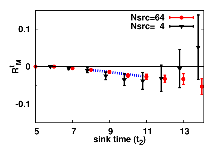
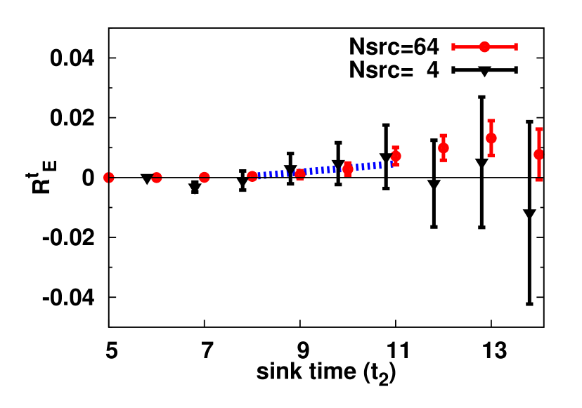
Figure 1: $R_{M}^{t}$ (left) and $R_{E}^{t}$ (right) with $\kappa_{ud}=0.13760$, $N_{src}=64$ (circles) and $N_{src}=4$ (triangles), plotted against the nucleon sink time $t_{2}$. The dashed line is the linear fit where the slope corresponds to the form factor.

The formulas for Sachs electric (magnetic) form factors $G_{E}^{s}$ ($G_{M}^{s}$) are given by

$$R_{\mu}^{\pm}(\Gamma_{\rm pol}^{\pm})\equiv\frac{{\rm Tr}\left[\Gamma_{\rm pol}^{\pm}\cdot\Pi^{\rm 3pt}_{J_{\mu}}(\vec{0},{t}_{2};\ \pm\vec{q},{t}_{1};\ -\vec{q},t_{0})\right]}{{\rm Tr}\left[\Gamma_{e}^{\pm}\cdot\Pi^{\rm 2pt}(\pm\vec{q},t_{1};\ t_{0})\right]}\cdot\frac{{\rm Tr}\left[\Gamma_{e}^{\pm}\cdot\Pi^{\rm 2pt}(\vec{0},t_{1};\ t_{0})\right]}{{\rm Tr}\left[\Gamma_{e}^{\pm}\cdot\Pi^{\rm 2pt}(\vec{0},t_{2};\ t_{0})\right]},$$ (2)

$$G_{E}^{s}(Q^{2})=\pm R_{\mu=4}^{\pm}(\Gamma_{\rm pol}^{\pm}=\Gamma_{e}^{\pm}),\qquad G_{M}^{s}(Q^{2})=\mp\frac{E^{q}_{N}+m_{N}}{\epsilon_{ijk}q_{j}}R_{\mu=i}^{\pm}(\Gamma_{\rm pol}^{\pm}=\Gamma_{k}^{\pm}),$$ (3)

where $J_{\mu}(x+\mu/2)=\frac{1}{2}\left[\bar{q}(x)(1-\gamma_{\mu})U_{\mu}(x)q(x+\mu)-\bar{q}(x+\mu)(1+\gamma_{\mu})U_{\mu}^{\dagger}(x)q(x)\right]$ is the point-split conserved vector operator, $\{i,j,k\}\neq 4$, $\Gamma_{e}^{\pm}\equiv(1\pm\gamma_{4})/2$ , $\Gamma_{k}^{\pm}\equiv(\pm i)/2\times(1\pm\gamma_{4})\gamma_{5}\gamma_{k}$ and $E^{q}_{N}\equiv\sqrt{m_{N}^{2}+\vec{q}^{\,2}}$. The upper sign corresponds to the forward propagation ($t_{2}\gg t_{1}\gg t_{0}$), and the lower sign corresponds to the backward propagation ($t_{2}\ll t_{1}\ll t_{0}$).

In Fig. 1, we plot typical figures for $R^{t}_{M,E}$, where $R^{t}_{M,E}\equiv\frac{1}{K_{M,E}^{\pm}}\sum_{t_{1}=t_{0}+t_{s}}^{t_{2}-t_{s}}R^{\pm}_{\mu}$ with $K_{M,E}^{\pm}$ being trivial kinematic factors in Eq. (3). Since $R^{t}_{M,E}={\rm const.}+t_{2}\times G_{M,E}^{s},$ the linear slope corresponds to the signal of the form factor. One can observe the significant S/N improvement by increasing $N_{src}$. In fact, the improvement is found to be nearly a factor of $\sqrt{N_{src}}$ (ideal improvement).

We then study the $Q^{2}$ dependence of the form factors. For the magnetic form factor, we employ the dipole form, $G_{M}^{s}(Q^{2})=G_{M}^{s}(0)/(1+Q^{2}/\Lambda^{2})^{2}$, where reasonable agreement with lattice data is observed. For the electric form factor, we employ $G_{E}^{s}(Q^{2})=g_{E}^{s}\cdot Q^{2}/(1+Q^{2}/\Lambda^{2})^{2}$, considering that $G_{E}^{s}(0)=0$ from the vector current conservation, and the pole mass $\Lambda$ is taken from the fit of magnetic form factor.

Finally, we perform the chiral extrapolation for the fitted parameters. Since our quark masses are relatively heavy, we consider only the leading dependence on $m_{K}$, which is obtained by heavy baryon chiral perturbation theory (HB$\chi$PT) chPT:hemmert . The chiral extrapolated results are $G_{M}^{s}(0)=-0.017(25)$, $\Lambda a=0.58(16)$, $\langle r_{s}^{2}\rangle_{M}\equiv-6\frac{dG_{M}^{s}}{dQ^{2}}|_{Q^{2}=0}=-7.4(71)\times 10^{-3}{\rm fm}^{2}$ and $g_{E}^{s}=0.027(16)$ (or $\langle r_{s}^{2}\rangle_{E}\equiv-6\frac{dG_{E}^{s}}{dQ^{2}}|_{Q^{2}=0}=-2.4(15)\times 10^{-3}{\rm fm}^{2}$).

We examine the systematic uncertainties in the result of form factors. For the ambiguity of $Q^{2}$ dependence, we reanalyze the data using the monopole form, and obtain the results which are consistent with those from the dipole form. For the uncertainties in chiral extrapolation, we test two alternative extrapolations smm:doi , and find that all results are consistent with each other. For the contamination from excited states, we employ the new projection operator smm:doi which eliminates the $S_{11}$ state, and conclude that such contaminations are negligible.

Our final result for the magnetic moment is $G_{M}^{s}(0)=-0.017(25)(07)$, where the first error is statistical and the second is systematic from uncertainties of the $Q^{2}$ extrapolation and chiral extrapolation. We also obtain $\Lambda a=0.58(16)(19)$ for dipole mass or $\tilde{\Lambda}a=0.34(17)(11)$ for monopole mass, and $g_{E}^{s}=0.027(16)(08)$. These lead to $G_{M}^{s}(Q^{2})=-0.015(23)$, $G_{E}^{s}(Q^{2})=0.0022(19)$ at $Q^{2}=0.1{\rm GeV}^{2}$, where error is obtained by quadrature from statistical and systematic errors. In Fig. 2, we plot $G_{M}^{s}(Q^{2})$, $G_{E}^{s}(Q^{2})$, where the shaded regions correspond to the square-summed error. Compared to the global analysis of the experimental data, e.g., $G_{M}^{s}(Q^{2})=0.29(21)$ and $G_{E}^{s}(Q^{2})=-0.008(16)$ at $Q^{2}=0.1{\rm GeV}^{2}$ pate08 , our results are consistent with them, with an order of magnitude smaller error smm:doi .

Figure 2: The chiral extrapolated results for $G_{M}^{s}(Q^{2})$ (left) and $G_{E}^{s}(Q^{2})$ (right) plotted with solid lines. Shaded regions represent the statistical and systematic error added in quadrature. Shown together are the lattice data for each $\kappa_{ud}$.

4 Second moment of the nucleon

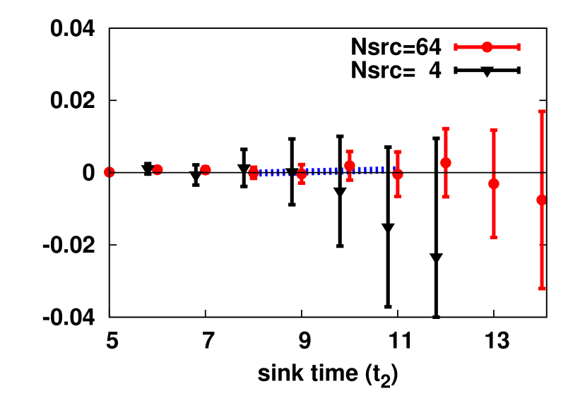
Figure 3:

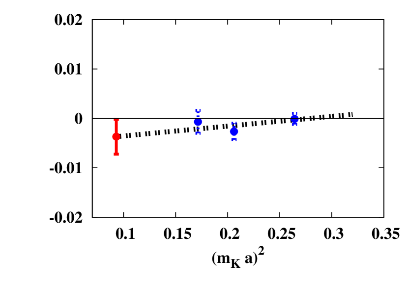
Figure 4:

Figure 5: LEFT: The ratio of 3pt to 2pt with $\kappa_{ud}=0.13760$, $N_{src}=64$ (circles) and $N_{src}=4$ (triangles), plotted against the nucleon sink time $t_{2}$. The dashed line is the linear fit where the slope corresponds to the second moment. RIGHT: The lattice bare results for the second moment at each valence quark mass $\kappa_{ud}$ for the nucleon, plotted against $(m_{K}a)^{2}$. The dashed line corresponds to the linear chiral extrapolation, and the red point is the chiral extrapolated result.

The (asymmetry of) strangeness second moment of the nucleon $\langle x^{2}\rangle_{s-\bar{s}}=\int_{0}^{1}dxx^{2}(s(x)-\bar{s}(x))$ can be obtained by

$$\frac{{\rm Tr}\left[\Gamma^{\pm}_{e}\cdot\Pi^{\rm 3pt}_{T_{4ii}}(\pm\vec{p},t_{2};\ \vec{0},t_{1};\ \pm\vec{p},t_{0})\right]}{{\rm Tr}\left[\Gamma^{\pm}_{e}\cdot\Pi^{\rm 2pt}(\pm\vec{p},t_{2};\ t_{0})\right]}=\pm p_{i}^{2}\cdot\langle x^{2}\rangle_{s-\bar{s}},$$ (4)

with the three-index operator defined as

$$T_{4ii}\equiv-\frac{1}{3}\left[\bar{q}\gamma_{4}\overleftrightarrow{D}_{i}\overleftrightarrow{D}_{i}q+\bar{q}\gamma_{i}\overleftrightarrow{D}_{4}\overleftrightarrow{D}_{i}q+\bar{q}\gamma_{i}\overleftrightarrow{D}_{i}\overleftrightarrow{D}_{4}q\right],$$ (5)

where $i\neq 4$, and the upper (lower) sign corresponds to the forward (backward) propagation as before.

In Fig. 5 (left), we plot the ratio of 3pt to 2pt for $\langle x^{2}\rangle_{s-\bar{s}}$ in terms of $t_{2}$ for $\kappa_{ud}=0.13760$, $\vec{p}^{\,2}=(2\pi/La)^{2}$, where the summation of operator insertion time $t_{1}$ is taken as was done for the form factor analysis. Note that the linear slope corresponds to the signal for $\langle x^{2}\rangle_{s-\bar{s}}$. One can clearly see that increasing $N_{src}$ reduces the error bar significantly again (about a factor of $\sqrt{N_{src}}$, i.e., almost ideally). In Fig. 5 (right), we plot the bare value of the $\langle x^{2}\rangle_{s-\bar{s}}$ in terms of $(m_{K}a)^{2}$, and perform the chiral extrapolation. We find that the result at each $\kappa_{ud}$ and the chiral extrapolated result are basically consistent with zero within the error-bar. For the final quantitative result, it is necessary to take the renormalization factor into account. Systematic uncertainties have to be examined as well. The study along this line is in progress.

References

(1)
S.-J. Dong, K.-F. Liu and A.G. Williams,
Phys. Rev. D 58, 074504 (1998).
(2)
N. Mathur and S.-J. Dong,
Nucl. Phys. Proc. Suppl. 94, 311 (2001);
ibid., 119, 401 (2003).
(3)
R. Lewis, W. Wilcox and R.M. Woloshyn,
Phys. Rev. D 67, 013003 (2003).
(4)
S.-J. Dong and K.-F. Liu,
Phys. Lett. B 328, 130 (1994).
(5)
C. Thron, S.-J. Dong, K.-F. Liu and H.P. Ying,
Phys. Rev. D 57, 1642 (1998).
(6)
M. Deka et al., Phys. Rev. D 79, 094502 (2009).
(7)
T. Doi et al. (QCD Collab.),
Phys. Rev. D 80, 094503 (2009).
(8)
T. Doi et al. (QCD Collab.),
PoS (LAT2008), 163 (2008),
T. Doi et al. (QCD Collab.),
PoS (LAT2009), 134 (2009).
(9)
T. Ishikawa et al.,
PoS (LAT2006), 181 (2006);
T. Ishikawa et al.,
Phys. Rev. D 78, 011502(R) (2008).
(10)
T.R. Hemmert et al.,
Phys. Lett. B 437, 184 (1998);
ibid.,
Phys. Rev. C 60, 045501 (1999).
(11)
S.F. Pate, D.W. McKee and V. Papavassiliou,
Phys. Rev. C 78, 015207 (2008).
(12)
R.G. Edwards and B. Joó,
Nucl. Phys. Proc. Suppl. 140, 832 (2005);
C. McClendon,
http://www.jlab.org/~edwards/qcdapi/reports/dslash_p4.pdf