Spin-polarized currents in double and triple quantum dots driven by ac magnetic fields

Abstract

We analyze transport through both a double quantum dot and a triple quantum dot with inhomogeneous Zeeman splittings in the presence of crossed dc and ac magnetic fields. We find that strongly spin-polarized current can be achieved by tuning the relative energies of the Zeeman-split levels of the dots, by means of electric gate voltages: depending on the energy level detuning, the double quantum dot works either as spin-up or spin-down filter. We show that a triple quantum dot in series under crossed dc and ac magnetic fields can act not only as spin-filter but also as spin-inverter.

I Introduction

A key aim in spintronics is the realization of spin-based quantum information devices, where coherent electron spin manipulation is a fundamental issue.loss ; cota In semiconductor quantum dots, coherent electron spin manipulation can be realized by electron spin resonance (ESR), where an oscillating magnetic field is applied to the sample in order to rotate the electron spin.koppens ; loss1 ; rafa ; levi ; danon ; busl Together with ESR, electron dipole spin resonance techniques — which combine ac electric fields with spin-orbit interactionnovak or with a dc magnetic field gradientpioro — have been implemented in order to measure coherent rotations of one single electron spinkoppens ; novak in double quantum dots (DQDs). Coherent spin rotations of one single spin have also been proposed theoretically in triple quantum dots (TQDs)buslphyse under crossed ac and dc magnetic fields.

In ESR experiments in quantum dot arrays, an important issue is to individually address the electron spin in each quantum dot. To this end, it has been proposed to tune the Zeeman splitting, in order to manipulate the electron spin independently in each dot.coish The Zeeman splitting in a quantum dot is determined by the intensity of the applied dc magnetic field and the electron g factor, $\Delta_{\text{Z}}=g\mu_{\text{B}}B_{\text{dc}}$. Hence different Zeeman splittings can occur in quantum dot arrays where the dots have different g factors, or as well by applying different magnetic fields to each quantum dot. Both alternatives have been realized experimentally very recently: vertical DQDs made out of different materials — e.g. GaAs and InGaAs — show different g factorshuang and on the other hand, in a sample with a spatially homogeneous g factor, an additional micro-ferromagnet placed nearby creates a different external magnetic field $B_{\text{dc}}$ in each dot.pioro

The next logic step from DQDs to networks of quantum dots is a TQD, in linear or triangular arrangement. Both versions have been realized experimentally in the last few years,ludwig ; haug ; gaudreau where tunneling spectroscopy and stability diagram measurements have been performed in order to gain a deeper insight into the electronic configurations in TQDs, which is necessary for potential three-spin qubit applications. On the theoretical side, next to fundamental studies of their eigenenergy spectrum,hawrylak TQDs have attracted interest mostly in a triangular arrangement, where the system symmetry gives rise to fundamental coherence phenomena. In this context, so-called “dark states”emary ; christina ; busl and Aharonov-Bohm oscillationsbusl ; hawrylakAB have been studied. TQDs have been used as a testing ground for Kondo physicskondo and have been proposed as current rectifiersvidan ; bulka and spin-entanglers.saraga

In the present work, we are interested in single electron manipulation, and therefore study theoretically transport through both double and triple quantum dots. We calculate the current and current spin polarization through a DQD and a linear TQD array exposed to crossed dc and ac magnetic fields. We consider an inhomogeneous dc magnetic field that produces different Zeeman splittings in the dots, while the g factor is the same in both dots. For DQDs, a regime is considered where the system is occupied either by zero or one electron. For TQDs, the corresponding features are discussed for one or two electrons in the system. With the single electron spin levels resolved in each quantum dot, interdot tunneling is governed by definite spin selection rules, i.e. tunneling from one dot to the other is only possible when two equal spin levels are aligned. However, when an ac magnetic field is applied, it rotates the spin and allows for spin-flip processes along the tunneling that can lead to new features in the current. This effect of an ac magnetic field has been explored previously in a DQD,koppens where the authors report single electron spin rotations by a combination of an ac magnetic field and sharp electric pulses.

In our work, as will be discussed in more detail below, we will focus our attention on the polarizing effect of an ac field, i.e. we will show that the combination of inhomogeneous dc and ac magnetic fields in DQDs and TQDs allows for the creation of spin-polarized currents and thus for the design of spin-filters and spin-inverters.

The paper is organized as follows: In section II we introduce the model and the technique used to calculate transport through a DQD and TQD. Section III discusses in detail the results of this paper. In section III.1 we first briefly review the main result of a related experimental work that has recently been reported in the literature and is important for further understanding. We then proceed in the following paragraphs III.2 - III.4 with a detailed analysis of the main results of this paper, namely the spin-polarized currents produced by a combination of dc and ac magnetic fields at certain interdot level detunings. The role of the system parameters involved in the polarization mechanism — Zeeman splitting difference, ac field amplitude and frequency and interdot tunneling amplitude — is discussed. In section III.5 we present the corresponding results obtained for a TQD. We end with a summary of the main results in section IV.

II Model and technique

We consider a quantum dot array as shown schematically in Fig. 1. The dots are coupled to each other coherently by a tunneling amplitude $t_{\text{ij}}$ and are weakly connected to source and drain contacts by rates $\Gamma_{\text{L}}$ and $\Gamma_{\text{R}}$. The total Hamiltonian of the system is:

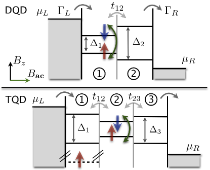
Figure 1: (Color online) Schematic diagram of a DQD (above) and TQD (below) exposed to crossed dc ($B_{\text{dc}}$) and ac ($B_{\text{ac}}$) magnetic fields. The electron spin is rotated once the ac frequency matches the Zeeman splitting in one of the dots. In the TQD, one electron is confined in the left dot (dot 1), such that only an electron with opposite spin can enter the TQD. The dots are coupled coherently by tunneling amplitudes $t_{\text{ij}}$ and incoherently to leads by rates $\Gamma_{\text{L}}$ and $\Gamma_{\text{R}}$.

$$\mathcal{H}=\mathcal{H}_{\text{Dots}}^{0}+\mathcal{H}_{t_{\text{ij}}}^{0}+\mathcal{H}_{\text{B}}^{0}(t)+\mathcal{H}_{\text{T}}+\mathcal{H}_{\text{Leads}},$$ (1)

where the individual terms are

$$\mathcal{H}_{\text{Dots}}^{0} =\sum_{i\sigma}\xi_{i\sigma}\hat{c}^{\dagger}_{i\sigma}\hat{c}_{i\sigma}+\sum_{i}U_{i}\hat{n}_{i\uparrow}\hat{n}_{i\downarrow}+\frac{1}{2}\sum_{i\neq j}V\hat{n}_{i}\hat{n}_{j}$$

$$\mathcal{H}_{t_{\text{ij}}}^{0} =-\sum_{ij\sigma}t_{\text{ij}}(\hat{c}^{\dagger}_{i\sigma}\hat{c}_{j\sigma}+\hat{c}^{\dagger}_{j\sigma}\hat{c}_{i\sigma})$$

$$\mathcal{H}_{\text{Leads}} =\sum_{l\in{L,R},k\sigma}\epsilon_{lk\sigma}\hat{d}^{\dagger}_{lk\sigma}\hat{d}_{lk\sigma}$$ (2)

$$\mathcal{H}_{\text{T}} =\sum_{l\in{L,R},k\sigma}\gamma_{l}(\hat{d}^{\dagger}_{lk\sigma}\hat{c}_{l\sigma}+\hat{c}^{\dagger}_{l\sigma}\hat{d}_{lk\sigma}).$$

The first term, $\mathcal{H}_{\text{Dots}}^{0}$, describes an isolated array of quantum dots, with electrons coupled electrostatically. Here, $\xi_{i}$ stands for the single energy spectrum of an electron located in dot $i$, and $U_{i}$ and $V$ are are the intra- and the inter-dot Coulomb repulsion respectively. $\mathcal{H}_{t_{\text{ij}}}^{0}$ describes the coherent tunneling between the dots, which in the case of a DQD is given by $t_{12}$ and in a TQD by $t_{12}$ and $t_{23}$. The quantum dot array is coupled to leads which are described by $\mathcal{H}_{\text{Leads}}$, and the coupling of the array to the leads is given by $\mathcal{H}_{\text{T}}$. The magnetic field Hamiltonian consists of two parts, coming from a dc field $B_{\text{dc}}$ in $z$-direction, and an ac field $B_{\text{ac}}$ applied in $xy$-direction:

$$\mathcal{H}_{\text{B}}^{0}(t)=\sum_{i}\left[\Delta_{i}S_{zi}+B_{\text{ac}}(\cos(\omega t)S_{xi}+\sin(\omega t)S_{yi})\right],$$ (3)

being ${\bf S}_{i}=\frac{1}{2}\sum_{\sigma\sigma^{\prime}}\hat{c}^{\dagger}_{i\sigma}\sigma_{\sigma\sigma^{\prime}}\hat{c}_{i\sigma^{\prime}}$ the spin operator of the $i$th dot, and the sum running over index $i=1,2$ for the DQD and $i=1,2,3$ for the TQD. $B_{\text{dc}}$ has a different intensity in each dot and thus produces different Zeeman splittings $\Delta_{i}=g\mu B_{\text{dc}_{i}}$, while we consider the dots with equal g factor. $B_{\text{ac}}$ induces spin rotations when its frequency fulfills the resonance condition $\omega=\Delta_{i}$. The time-dependent Hamiltonian can be transformed by means of a unitary transformationrafa ; busl $U(t)=\text{exp}(-i[\omega t\sum_{i}S_{zi}])$ into the rotating reference frame. The resulting time-independent Hamiltonian is then:

$$\mathcal{H}_{\text{B}}^{0}=\sum_{i}\left[(\Delta_{i}-\hbar\omega)S_{zi}+B_{\text{ac}}S_{xi}\right].$$ (4)

The dynamics of the system is given by the time evolution of the reduced density matrix elements $\rho_{mn}$, whose equations of motion read, within the Born-Markov-approximation:

$$\dot{\rho}_{mn}(t)= -i\langle m|[\mathcal{H}_{\text{Dots}}^{0}+\mathcal{H}_{t_{\text{ij}}}^{0}+\mathcal{H}_{\text{B}}^{0},\rho]|n\rangle$$ (5)

$$+\sum_{k\neq{n}}(\Gamma_{nk}\rho_{kk}-\Gamma_{kn}\rho_{nn})\delta_{mn}$$

$$-\Lambda_{mn}\rho_{mn}(1-\delta_{mn})$$

The commutator accounts for the coherent dynamics in the quantum dot array, tunneling to and from the leads is governed by transition rates $\Gamma_{mn}$ from state $|n\rangle$ to state $|m\rangle$, and decoherence due to interaction with the reservoir is considered in the term $\Lambda_{mn}=\frac{1}{2}\sum_{k}(\Gamma_{km}+\Gamma_{kn})$. The transition rates are calculated using Fermi’s golden rule:

$$\Gamma_{mn}=\sum_{l=L,R}\Gamma_{l} [f(E_{m}-E_{n}-\mu_{l})\delta_{N_{m},N_{n}+1}+$$

$$(1-f(E_{m}-E_{n}-\mu_{l}))\delta_{N_{m},N_{n}-1}],$$ (6)

where $E_{m}-E_{n}$ is the energy difference between states $|m\rangle$ and $|n\rangle$ of the isolated quantum dot array, and $\Gamma_{\text{L,R}}=2\pi\mathcal{D}_{\text{L,R}}|\gamma_{\text{L,R}}|^{2}$ are the tunneling rates for each lead. The density of states $\mathcal{D}_{\text{L,R}}$ and the tunneling couplings $\gamma_{\text{L,R}}$ are assumed to be energy independent. We set $\Gamma_{\text{L}}=\Gamma_{\text{R}}=\Gamma$.

We consider strong Coulomb repulsion, such that the DQD can be occupied with at most one extra electron. It is then described by a basis of 5 states, namely: $|0,0\rangle$, $|{\uparrow},0\rangle$, $|{\downarrow},0\rangle$, $|0,{\uparrow}\rangle$, $|0,{\downarrow}\rangle$. With a bias applied from left to right, current $I$ flows whenever dot 2 is occupied:

$$I_{\text{DQD}}=\Gamma(\rho_{|0,{\uparrow}\rangle}+\rho_{|0,{\downarrow}\rangle})$$ (7)

In the TQD, one electron is confined in the left dot (dot 1, see Fig. 1, lower panel), and the chemical potential of the left lead is such that only an electron with the opposite spin can enter the TQD. Considering here as well strong Coulomb repulsion, we allow only for one additional electron to enter the TQD. The full two-electron basis for the TQD contains fifteen two-electron states, and one zero- and six one-electron states. For the scope of this paper, it is sufficient to look at transport around the triple point $(2,0,0)\leftrightarrow(1,1,0)\leftrightarrow(1,0,1)$. The number of relevant basis states is then reduced to eleven, which are

• 1-electron states: $|{\uparrow},0,0\rangle$, $|{\downarrow},0,0\rangle$

• 2-electron states: $|{\uparrow},{\uparrow},0\rangle$, $|{\uparrow},{\downarrow},0\rangle$, $|{\downarrow},{\uparrow},0\rangle$, $|{\downarrow},{\downarrow},0\rangle$
  $|{\uparrow},0,{\uparrow}\rangle$, $|{\uparrow},0,{\downarrow}\rangle$, $|{\downarrow},0,{\uparrow}\rangle$, $|{\downarrow},0,{\downarrow}\rangle$
  $|{\uparrow}{\downarrow},0,0\rangle$.

The current from left to right through the TQD is calculated summing over all states that include an electron in the right dot (dot 3):

$$I_{\text{TQD}}=\Gamma\left(\rho_{|{\uparrow},0,{\uparrow}\rangle}+\rho_{|{\uparrow},0,{\downarrow}\rangle}+\rho_{|{\downarrow},0,{\uparrow}\rangle}+\rho_{|{\downarrow},0,{\downarrow}\rangle}\right)$$ (8)

The spin-resolved currents hence are

$$I_{\uparrow} =\Gamma\left(\rho_{|{\uparrow},0,{\uparrow}\rangle}+\rho_{|{\downarrow},0,{\uparrow}\rangle}\right)$$

$$I_{\downarrow} =\Gamma\left(\rho_{|{\uparrow},0,{\downarrow}\rangle}+\rho_{|{\downarrow},0,{\downarrow}\rangle}\right).$$ (9)

The spin polarization of the current is defined as

$$P=\frac{I_{\uparrow}-I_{\downarrow}}{I_{\uparrow}+I_{\downarrow}},$$ (10)

where $I_{\uparrow}(I_{\downarrow})$ is the $\uparrow$($\downarrow$)-current.

III Results

III.1 Undriven case: $B_{\text{ac}}=0$

Let us now start to describe transport through a DQD (see Fig. 1, upper panel). In this section we will reproduce within our theoretical framework the results recently reported by Huang et al..huang The authors have shown that in transport through DQDs with different Zeeman splittings a so-called spin bottleneck situation can occur: When either ${\uparrow}$- or ${\downarrow}$-levels are aligned, transport is suppressed, whereas the current is largest in the configuration where the interdot level detuning $\epsilon$ is set to half the Zeeman energy difference.

Applying a dc magnetic field in z-direction produces a Zeeman splitting $\Delta_{z}$, which we consider inhomogeneous: $\Delta_{1}\neq\Delta_{2}$, and $\delta=\Delta_{2}-\Delta_{1}$. If an electron tunnels onto the ${\uparrow}$(${\downarrow}$)-level in dot 1 that is far from resonance from the corresponding spin-level in dot 2, a spin blockade or bottleneck situation arises: Spin is conserved at tunneling, so the electron remains in dot 1 without being able to tunnel to dot 2. This blockade is only relieved by a finite level broadening and coupling to the leads. The maximal current occurs then for the most symmetric level arrangement, that is when neither ${\uparrow}$- nor ${\downarrow}$-levels are in resonance, but when they are symmetrically placed around each other (see Fig. 2). Increasing the Zeeman splitting difference $\delta$ maintains the bottleneck situation, but the central current decreases, since it is a consequence of the level hybridization of the same spin-levels due to tunneling. Hence, the further separated they are, the less current flows. Notice that the current only depends on the Zeeman splitting difference $\delta$ and not on the absolute values.

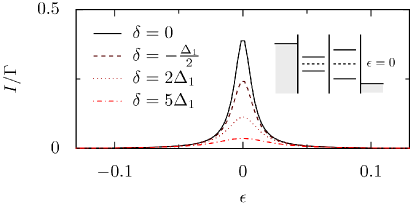
Figure 2: (Color online) Current $I$ versus detuning $\epsilon$ in an undriven DQD with different Zeeman splittings. Here maximal current flows, when $\epsilon=0$, and this central current decreases for increasing $\delta$, since then parallel spin-levels are more separate. Parameters ($e=\hbar=1$, in meV): $t_{\text{12}}=0.005$, $\Gamma=0.001$, $\Delta_{1}=0.025$ ($B_{\text{dc}}\approx 1$T), and the current $I$ is normalized in units of the hopping $\Gamma$ to the leads.

Interdot tunneling conserves spin and the current through the sample is completely unpolarized. In ac magnetic fields however, the electron spin undergoes rotations and the spin selection rules thus do not apply any more. For certain detunings, this will lead to spin-polarized currents, as we will see in the next section.

III.2 Resonance condition: $\omega=\Delta_{1}$

With a circularly polarized ac magnetic field $B_{\text{ac}}$ applied to the DQD, the transformed Hamiltonian $\mathcal{H}^{0}$ reads:

$$\mathcal{H}^{0}=\left(\begin{array}[]{cccc}-\frac{\Delta_{1}}{2}+\frac{\omega}{2}&\frac{B_{\text{ac}}}{2}&-t_{\text{12}}&0\\ \frac{B_{\text{ac}}}{2}&\frac{\Delta_{1}}{2}-\frac{\omega}{2}&0&-t_{\text{12}}\\ -t_{\text{12}}&0&-\frac{\Delta_{2}}{2}+\frac{\omega}{2}-\epsilon&\frac{B_{\text{ac}}}{2}\\ 0&-t_{\text{12}}&\frac{B_{\text{ac}}}{2}&\frac{\Delta_{2}}{2}-\frac{\omega}{2}-\epsilon\end{array}\right),$$ (11)

where $\epsilon$ is the detuning between dot 1 and dot 2.

For the ease of its analysis, Hamiltonian (11) can be seen as a a pair of two-level systems coupled by $t_{12}$. In a two-level system, the important physical quantities are the energy difference (“detuning”) of the two levels and the coupling between them. In the present case, note that $t_{\text{12}}$ couples only levels with the same spin, which are detuned by $\pm\delta/2+\epsilon$, where $\delta=\Delta_{2}-\Delta_{1}$. Moreover, within each dot the different spin-levels are coupled by $B_{\text{ac}}/2$ and “detuned” by $\omega-\Delta_{1,2}$ (see diagonal elements in (11)). Therefore, depending on the ac frequency $\omega$, the energy levels in either left or right dot are renormalized to the same energy. In the other dot however, since there $\omega\gtrless\Delta_{i}$, the renormalized splitting between the spin-levels becomes smaller when $\omega<\Delta_{i}$ or bigger for $\omega>\Delta_{i}$. We will focus first on the resonance condition $\omega=\Delta_{1}$, as it is the most relevant here.

In order to understand the effect of $B_{\text{ac}}$ on the system, let us look at the eigenstates of the isolated dots 1 and 2. In dot 1, since $\omega=\Delta_{1}$, the eigenstates are $|\psi_{1}\rangle^{\pm}=\frac{1}{\sqrt{2}}(|{\uparrow}_{1}\rangle\pm|{\downarrow}_{1}\rangle)$ and their eigenenergies differ by $B_{\text{ac}}$. In dot 2 however, since it is out of resonance, the eigenstates depend both on $\delta$ and $B_{\text{ac}}$:

$$|\psi_{2}\rangle^{\pm}=\frac{1}{N^{\pm}}(-\frac{\delta\pm\sqrt{B_{\text{ac}}^{2}+\delta^{2}}}{B_{\text{ac}}}|\uparrow_{2}\rangle+|\downarrow_{2}\rangle)$$ (12)

Here $N^{\pm}=\sqrt{2}/B_{\text{ac}}\left(\sqrt{B_{\text{ac}}^{2}+\delta^{2}\pm\delta\sqrt{B_{\text{ac}}^{2}+\delta^{2}}}\right)$ are the normalization factors. The eigenenergies associated to these states are separated by $\sqrt{B_{\text{ac}}^{2}+\delta^{2}}$. It is straightforward to show that for $B_{\text{ac}}\ll\delta$, the eigenstates in dot 2 are almost pure ${\uparrow}$(${\downarrow}$)-states, i.e. the spin-mixing is weak. Regarding the detuning $\epsilon$, we distinguish three different level arrangements, see Fig. 3, upper panel: In case I, the $\uparrow$- and $\downarrow$-levels in dot 1 are aligned with the $\uparrow$-level in dot 2, case II is the symmetric situation, and in case III the levels in dot 1 are in resonance with the $\downarrow$-level in dot 2.

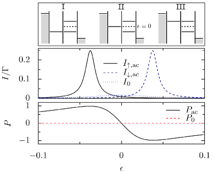
Figure 3: (Color online) Upper panel: Energy level distribution for different detunings $\epsilon$ in a DQD driven by $B_{\text{ac}}$. When $\omega=\Delta_{1}$, the levels in dot 1 renormalize to the same energy (their eigenenergies are split by $B_{\text{ac}}$, see text), and the levels in dot 2 get closer or farther apart than in the undriven case. Middle panel: Spin-resolved currents $I_{\uparrow}$ and $I_{\downarrow}$ vs. detuning $\epsilon$. At $\epsilon\approx\pm\delta/2$, the current is strongly $\uparrow$($\downarrow$)-polarized, compared to the undriven current $I_{0}$. Lower panel: Polarization $P$ versus the detuning $\epsilon$. Note the strong polarization ($P\approx\pm 1$) around $\epsilon\approx\pm\delta/2$. Parameters in meV ($e=\hbar=1$): $\Gamma=0.001$, $t_{\text{12}}=0.005$, $B_{\text{ac}}=0.005$ ($\approx 0.2$T), $\Delta_{1}=0.025$ ($B_{\text{z}1}\approx 1$T), $\Delta_{2}=0.1$.

In Fig. 3, lower panels, we plot the current $I$ through the driven DQD and the polarization $P$ as a function of the level detuning $\epsilon$. It shows two peaks at $\epsilon\approx\pm\delta/2$. At these lateral peaks, corresponding to case I and III, the current is strongly spin-polarized: an electron in dot 1 is rotated by the ac field which breaks the spin bottleneck and the electron can thus tunnel to dot 2, where the spin-levels are almost pure, or — speaking in terms of the rotating field — the ac frequency in dot 2 is far off resonance and cannot rotate the electron there. We thus arrive at one of the main result of this paper: under the condition $\omega=\Delta_{1}$, dot 2 acts as a spin-filter, and it depends on $\epsilon$, whether it filters $\uparrow$- or $\downarrow$-electrons. Notice that the current $I$ only depends on $\delta$ and not on the absolute values $\Delta_{1,2}$.

For the purpose of a spin-filter, one has to answer the question as to how reliable the mechanism is, and how it depends on the different system parameters. Both strong polarization and measurable currents are desirable. Here, we discuss the sensibility of the spin filtering mechanism towards the interplay between tunneling $t_{\text{12}}$, ac field intensity $B_{\text{ac}}$ and Zeeman splitting difference $\delta$.

In order to get more insight into the problem, we obtain the current $I$ analytically for certain limits: At symmetric detuning $\epsilon=0$ (case II), the current is unpolarized and reads

$$\frac{I_{0}}{\Gamma}=\frac{4t_{\text{12}}^{2}(4B_{\text{ac}}^{2}+\Gamma^{2}+\delta^{2})}{4B_{\text{ac}}^{2}(\Gamma^{2}+10t_{\text{12}}^{2})+(\Gamma^{2}+\delta^{2})(\Gamma^{2}+10t_{\text{12}}^{2}+\delta^{2})}.$$ (13)

$I_{0}$ decreases for large $\delta$ and increases with growing $B_{\text{ac}}$. In the limit of very large $t_{\text{12}}$, the total current $I$ saturates to $I/\Gamma(t_{\text{12}}\to\infty)=2/5$. For the limiting cases of $B_{\text{ac}}$ we get

$$\lim_{B_{\text{ac}}\to 0}\frac{I_{\uparrow,\downarrow}}{\Gamma} =\frac{2t_{\text{12}}^{2}}{\Gamma^{2}+10t_{\text{12}}^{2}+4\epsilon^{2}+\delta^{2}}$$ (14)

$$\lim_{B_{\text{ac}}\to\infty}\frac{I_{\uparrow,\downarrow}}{\Gamma} =\frac{2t_{\text{12}}^{2}}{\Gamma^{2}+10t_{\text{12}}^{2}+4\epsilon^{2}}.$$ (15)

For $B_{\text{ac}}\to 0$, i.e. in the undriven case, the current is unpolarized and maximal at $\epsilon=0$ and decreases for growing $\delta$, see Eq.(14). Notice that in the opposite limit, i.e. for large $B_{\text{ac}}$ (Eq.(15)), the current is the same as in the undriven case for $\delta=0$. In this case, the difference of the eigenenergies in each isolated dot becomes $B_{\text{ac}}$ in both dots and the spins are mixed almost equally strongly. The polarized side-peaks therefore disappear in favor of the unpolarized central current peak, see also Eq.(13).

Numerical analysis for intermediate field and tunneling amplitude yields that when $t_{\text{12}}$ and $B_{\text{ac}}$ become of the order of $\delta$, the current is practically unpolarized. We find that at $B_{\text{ac}}/t_{12}\approx 1.5$, the polarization is strongest, when $\delta/t_{12}$ is at least one order of magnitude bigger than $B_{\text{ac}}/t_{12}$. It can be shown numerically that for $t_{\text{12}},B_{\text{ac}}\ll\delta$ the position $\epsilon$ of the side-peaks is $\epsilon\approx\pm\delta/2$. The larger $\delta$, the further separated the peaks corresponding to $I_{\uparrow}$ and $I_{\downarrow}$. As a consequence, also the polarization is stronger for large $\delta$, since the overlap of the spin-resolved currents tends to zero.

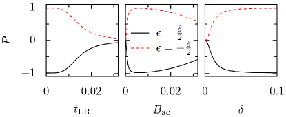
Figure 4: (Color online) Polarization $P$ versus $t_{\text{12}}$ , $B_{\text{ac}}$ and $\delta$ in ac-driven DQD at detuning $\epsilon=\pm\delta/2$ for $\omega=\Delta_{1}$: Left and middle panel: For both small $t_{\text{12}}$ and $B_{\text{ac}}$, spin-polarized current flows. $|P|$ becomes smaller as $B_{\text{ac}}$ and $t_{\text{12}}$ grow. Right panel: $P$ is zero at $\delta=0$ and increases with $\delta$. Parameters see Fig. 3.

In order to illustrate the effect of tunneling $t_{\text{12}}$, ac field intensity $B_{\text{ac}}$ and Zeeman splitting difference $\delta$ on the polarization $P$, we calculate $P$ at $\epsilon=\pm\delta/2$ (Fig. 4). In the left and middle panel, one can appreciate that for both small $t_{\text{12}}$ and $B_{\text{ac}}$, $P\approx\pm 1$, and it becomes smaller as $t_{\text{12}}$ and $B_{\text{ac}}$ increase (for constant $\delta$). The right panel in Fig. 4 shows the polarization for increasing $\delta$: the larger $\delta$, the stronger $P$ .

III.3 Resonance condition: $\omega=\Delta_{2}$

When the ac field instead fulfills the resonance condition $\omega=\Delta_{2}$, the energy renormalization due to $\omega$ is reversed in the two dots as compared to $\omega=\Delta_{1}$, and now the energy levels in dot 2 become degenerate. The analytical limits described for $\omega=\Delta_{1}$ hold here as well: For large $t_{\text{12}}$ and $B_{\text{ac}}$, the current becomes unpolarized, and at $\epsilon=0$, it follows Eq.(13). However, out of these limits, transport behavior here is very different from the case $\omega=\Delta_{1}$: At detunings $\epsilon\approx\pm\delta/2$, spin bottleneck occurs similar as was shown in the undriven case: Since dot 1 is out of resonance, the ac field can not rotate the electron there, hence tunneling to dot 2 is strongly suppressed. The maximal (unpolarized) current then flows for $\epsilon=0$ and no side-peaks appear.

In summary, at $\omega\approx\Delta_{1}$, dot 2 can always act as a spin-filter. The mixing of $\uparrow$- and $\downarrow$-states due to the ac field is always stronger in dot 1 than in dot 2, no matter if $\Delta_{1}\gtrless\Delta_{2}$. The ac field mixes $\uparrow$- and $\downarrow$-states in dot 1 such that at $\epsilon\approx\pm\delta/2$, the electron tunnels onto the almost pure $\uparrow$- or $\downarrow$-levels in dot 2, which thus filters the spin and gives rise to spin-polarized currents. This is opposed to the case $\omega=\Delta_{2}$: Here, due to spin bottleneck, tunneling to dot 2 is only possible around $\epsilon=0$, where the current is totally unpolarized. This behavior is shown in Fig. 5 in two density plots of the current $I$ versus detuning $\epsilon$ and $\delta=\Delta_{2}-\Delta_{1}$ for the two cases $\omega=\Delta_{1}$ (left) and $\omega=\Delta_{2}$ (right). In the left plot, one can clearly see the formation of the two spin-polarized current branches, which move far apart as $\delta$ and $\epsilon$ grow. In contrast to that, the right plot shows that current only flows for both $\epsilon=0$ and $\delta=0$, and no spin-polarized side-peaks arise.

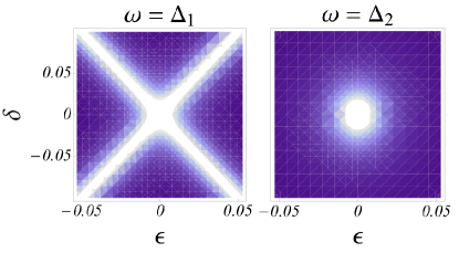
Figure 5: (Color online) Density plots of the current $I$ versus detuning $\epsilon$ and Zeeman splitting difference $\delta$. Left side: $\omega=\Delta_{1}$: For growing $\delta$ and $\epsilon$, the current $I$ splits off in two branches (light-colored regions), which are spin-polarized in opposite direction (cf. previous section). Right side: $\omega=\Delta_{2}$: Current flows only around $\delta=\epsilon=0$ (light-colored region); $P=0$. Parameters see Fig. 3.

III.4 Non-resonant driving

If the ac frequency does not match any of the Zeeman splittings $\Delta_{1,2}$, the effective finite Zeeman splittings are $\Delta_{1,2}^{*}=\Delta_{1,2}-\omega$. It is easy to prove that for $\omega=(\Delta_{1}+\Delta_{2})/2=\omega_{\text{s}}$, there is a “symmetric” situation, namely $\Delta_{1}^{*}=(\Delta_{1}-\Delta_{2})/2$, and $\Delta_{2}^{*}=-\Delta_{1}^{*}$. In this case, the mixing of the spin-states within each dot is equal in both dots, or in other words, both dots are equally far from resonance with the ac field. Regarding interdot tunneling, the levels are resonant at $\epsilon=0$, giving rise to one unpolarized current-peak. At all other detunings $\epsilon$, spin bottleneck avoids the formation of polarized side-peaks. In Fig. 6 we show the total current $I$ (upper left) and spin-resolved currents $I_{\uparrow}$ (upper middle), $I_{\downarrow}$ (upper right) vs. detuning $\epsilon$ and frequency $\omega$, for $\Delta_{1}<\Delta_{2}$. In order to appreciate the different current intensities, we plot in the lower panel the total current versus the detuning $\epsilon$ for the three relevant frequencies $\omega=\Delta_{1},\Delta_{2},\omega_{\text{s}}$. Note the regimes for $\omega$, as discussed in the previous sections: For $\omega=\Delta_{2}$, spin bottleneck only allows for a very weak and unpolarized current to flow around $\epsilon=0$. When the frequency matches the symmetric value $\omega_{\text{s}}$, at $\epsilon=0$ one sharp and unpolarized current peak arises, as predicted. Further decreasing of the frequency splits the current into two branches, which are enhanced and broadened as $\omega\approx\Delta_{1}$. The sidearms correspond to either $\uparrow$(middle panel)- or $\downarrow$(right panel)-electrons. For any off-resonant frequency, the current depends not only on $\delta$ as in the resonant case, but also on the absolute values $\Delta_{1,2}$. Hence the position of the side-peaks is not $\epsilon\approx\pm\delta/2$, but follows a different behavior. This explains the kink in Fig. 6 (upper panel) around $\omega=\Delta_{1}$.

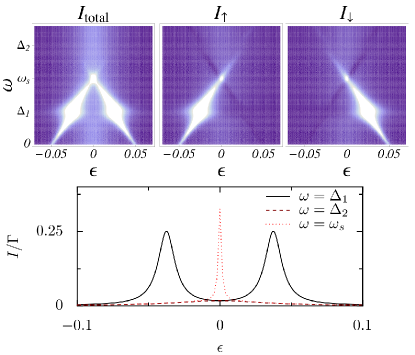
Figure 6: (Color online) Upper panel: Density plots of the total current (left) and spin-resolved currents $I_{\uparrow}$ (middle) and $I_{\downarrow}$ (right) vs. detuning $\epsilon$ and ac frequency $\omega$ for $\Delta_{1}<\Delta_{2}$. The lighter the color, the higher the current. Note that only very low current flows in the frequency range $\omega>\omega_{\text{s}}$ around $\epsilon=0$. At $\omega=\omega_{\text{s}}$ and $\epsilon=0$, one sharp unpolarized peak arises. Lowering $\omega$ further, the current splits into two arms and successively grows, until around $\omega=\Delta_{1}$, current is strongly enhanced and polarized, since the sidearms stem from either $\uparrow$- or $\downarrow$-electrons, see middle and right upper panel. Lower panel: Current versus $\epsilon$ for the three different situations $\omega=\Delta_{1}$, $\omega=\Delta_{2}$ and $\omega=\omega_{\text{s}}$. One can appreciate the big difference in the current intensities: Only for $\omega=\Delta_{1}$, polarized sidepeaks arise. For $\omega=\Delta_{2}$, current flows weakly around $\epsilon=0$ and for $\omega_{\text{s}}$, only at $\epsilon=0$ a sharp current peak appears. Parameters see Fig. 3.

We want to stress that, in the ac-driven DQD, spin-polarized currents can be achieved both for $\Delta_{1}>\Delta_{2}$ or $\Delta_{1}<\Delta_{2}$, since by varying the frequency $\omega$ one can always tune one Zeeman splitting to be smaller than the other, as schematically indicated by the renormalization of the energy levels due to $\omega$ (see Fig. 3, upper panel). In contrast to that, a static magnetic field set-up — for example, considering dc magnetic fields in $x$-directiontokura — would only produce polarized currents for $\Delta_{1}<\Delta_{2}$.

III.5 A triple quantum dot as spin-inverter

Now we want to implement the spintronic functionality of the spin-filter device towards a spin-inverter, and to this end we consider a TQD. Our goal is to produce spin-polarized incoming current $I_{\text{in}}$ and oppositely spin-polarized outgoing current $I_{\text{out}}$.

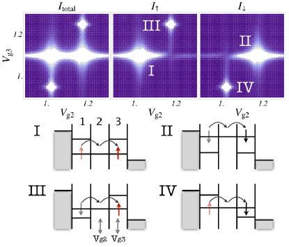
Figure 7: (Color online) Total current $I$ and spin-resolved currents $I_{\uparrow}$ and $I_{\downarrow}$ vs. gate voltages $V_{\text{g2}}$ and $V_{\text{g3}}$ applied to the central dot (dot 2) and the right dot (dot 3) in a TQD exposed to crossed $B_{\text{dc}}$ and $B_{\text{ac}}$. Here $\omega=\Delta_{2}$ and $\Delta_{1}=\Delta_{3}>\Delta_{2}$. Four relevant level configurations can occur due to adjustment of $V_{\text{g2}}$ and $V_{\text{g3}}$: in cases I and II, current through the TQD is polarized in one spin-direction, and in cases III and IV, the electron spin is inverted. In order not to overload the figure, we indicate only the spins of the incoming and outgoing electrons, but note that always one electron is confined in an off-resonant state in the left dot (dot 1, cf. Fig. 1). Parameters in meV ($e=\hbar=1$): $\Gamma=0.01$, $t_{\text{12, 23}}=0.01$, $B_{\text{ac}}=0.01$ ($\approx 0.4$T), $\Delta_{1}=\Delta_{3}=7\Delta_{2}$, $\Delta_{2}=0.025$ ($B_{\text{dc}}\approx 1$T), $U=1.0$.

We consider the TQD in a regime where only 2 electrons can be in the TQD at a time, and one electron is confined electrostatically in the left dot (dot 1, cf. Fig. 1, lower panel). This confinement is necessary to introduce spin correlations in the dot, such that only an electron with opposite spin can enter the TQD. The incoming current is then either $\uparrow$- or $\downarrow$-polarized, depending on the position of the energy levels in the adjacent dot. The ac field frequency $\omega$ is in resonance with the central dot (dot 2), $\omega=\Delta_{2}$, in order for the right dot (dot 3) to act as the filter dot. The TQD is here operated at the triple point $(2,0,0)\leftrightarrow(1,1,0)\leftrightarrow(1,0,1)$. We restrict the discussion for simplicity to the case where the Zeeman splittings are $\Delta_{1}=\Delta_{3}>\Delta_{2}$, although this condition is not necessary, as long as $\Delta_{1,3}\neq\Delta_{2}$.

From the previous sections we already know that depending on the detuning, the dot connected to the drain can act as $\uparrow$- or $\downarrow$-filter. In a TQD, there is one more degree of freedom compared to the DQD regarding the “detuning” between the dot levels. Without loss of generality, we can fix the energy level of dot 1, and move the energy levels of dot 2 and 3 (which is experimentally realized by applying gate voltages to the corresponding dots). Under these conditions, there are then four relevant energy level configurations, which are shown in Fig. 7, lower panel. In two of the configurations (I and II), the TQD acts as a spin-polarizer, and in the other two (III and IV) the electron spin is inverted. We hereby arrive at another important result of our work: A TQD can be tuned as both spin-polarizer and spin-inverter, by confining one electron in the left dot and adjusting the gate voltages at two of the three dots. Then electrons coming from the left lead can only enter with a distinct spin-polarization, which depends on the level position of the central dot. As the magnetic field $B_{{}_{\text{ac}}}$ is turned on with frequency $\omega=\Delta_{2}$, the electron spin coming from dot 1 is rotated in dot 2, whereas dot 1 and dot 3 due to their different Zeeman splittings are far off resonance from the ac field. Dot 3 then acts as spin-filter and, depending on the relative position of its energy levels with respect to dot 2, a ${\uparrow}$- or ${\downarrow}$-polarized current is produced, similar as in the DQD described in the previous sections.

We plot the total $I_{\text{total}}$ and spin-resolved currents $I_{\uparrow}$ and $I_{\downarrow}$ versus the two gate voltages applied to dot 2 and dot 3 in Fig. 7, together with sketches of the corresponding energy level distribution. In situations I and IV, dot 2 is energetically in resonance with the $\uparrow$-level in dot 1. Therefore, only $\uparrow$-electrons coming from the left lead will be able to tunnel to dot 2. Here they are inverted due to $\omega=\Delta_{2}$, where the renormalized energy levels have been depicted schematically as we did for the DQD. It depends then on the level position of dot 3, if the outgoing current is spin-up (case I) or spin-down (case IV) polarized. An analogue situation occurs for cases II and III: the energy level of dot 2 is such that only $\downarrow$-electrons can tunnel from dot 1 to dot 2. Again, after rotation due to the ac field in dot 2, in dot 3 the spin is filtered without inversion (case II) or inverted (case III).

IV Conclusions

In summary, we have analyzed spin current polarization in the transport through a DQD with one extra electron, and through a TQD with two extra electrons in the system. The quantum dot arrays are subjected to two different external magnetic fields: an inhomogeneous dc field, which produces different Zeeman splittings in the dot, and a time dependent ac field, that rotates the electron spin in one dot, when the resonance condition $\omega=\Delta_{\text{Z}}$ is fulfilled. For the DQD, we have analyzed both off-resonance and resonance conditions of the ac field with either one of the Zeeman splittings. Our results show that ac magnetic fields produce strongly spin-polarized current through a DQD depending on the detuning of the energy levels in the dots and on the resonance conditions.

Finally, we have proposed a TQD in series as both spin-polarizer and spin-inverter. As in a DQD, in a TQD different Zeeman splittings in the sample combined with a resonant ac frequency give way to spin-polarized currents. In addition, spin-polarized incoming current can be achieved, and thus the spin-polarizing mechanism can be extended to a spin-inversion mechanism. Our results show that dc and ac magnetic fields combined with gate voltages allow one to manipulate the current spin-polarization through DQDs and TQDs which are then able to work as a spin-filter and spin-inverter.

In spintronic devices at the nanometer scale an environment of nuclei introduces additional spin-flip processes that can lower the efficiency of the desired mechanism. In our set-up, we do not expect spin-flip processes due to hyperfine interaction to influence drastically on the results, because hyperfine spin-flip times are usually much longer than typical tunneling times in quantum dot arrays, especially in finite magnetic fields, where the hyperfine interaction is an inelastic process.

Therefore, the systems presented in this work are promising candidates for spintronic devices.

References

- (1) D. Loss and D. P. DiVincenzo, Phys. Rev. A 57, 120 (1998).
- (2) E. Cota, R. Aguado, and G. Platero, Phys. Rev. Lett. 94, 107202 (2005); R. Sánchez, E. Cota, R. Aguado, and G. Platero, Phys. Rev. B 74, 035326 (2006).
- (3) F.H.L. Koppens, C. Buizert, K.J. Tielrooij, I.T. Vink, K.C. Nowack, T. Meunier, L.P. Kouwenhoven, and L.M.K. Vandersypen, Nature 442, 766 (2006).
- (4) H.-A. Engel and D. Loss, Phys. Rev. B 65, 195321 (2002).
- (5) R. Sánchez, C. López-Monís, and G. Platero, Phys. Rev. B, 77, 165312 (2008).
- (6) M. S. Rudner and L. S. Levitov, Phys. Rev. Lett. 99, 246602 (2007).
- (7) J. Danon and Y. V. Nazarov, Phys. Rev. Lett. 100, 056603 (2008).
- (8) M. Busl, R. Sánchez, and G. Platero, Phys. Rev. B(R) 81, 121306 (2010); M. Busl, R. Sánchez, and G. Platero, Journal of Physics, Conference Series, 245, 012016 (2010).
- (9) K. C. Nowack, F. H. L. Koppens, Yu. V. Nazarov, L. M. K. Vandersypen, Science 318, 1430 (2007).
- (10) E. A. Laird, C. Barthel, E. I. Rashba, C. M. Marcus, M. P. Hanson, and A. C. Gossard, Phys. Rev. Lett. 99, 246601 (2007); M. Pioro-Ladrière, T. Obata, Y. Tokura, Y.-S. Shin, T. Kubo, K. Yoshida, T. Taniyama, and S. Tarucha, Nature Phys. 4, 776 (2008).
- (11) M. Busl, R. Sánchez, and G. Platero, Physica E, 42, 830 (2010).
- (12) W. A. Coish and D. Loss, Phys. Rev. B 75, 161302(R) (2007).
- (13) S.M. Huang, Y. Tokura, H. Akimoto, K. Kono, J. J. Lin, S. Tarucha, and K. Ono, Phys Rev. Lett. 104, 136801 (2010).
- (14) D. Schröer, A. D. Greentree, L. Gaudreau, K. Eberl, L. C. L. Hollenberg, J. P. Kotthaus, and S. Ludwig, Phys. Rev. B 76, 075306 (2007).
- (15) M. C. Rogge and R. J. Haug, Phys. Rev. B 77, 193306 (2008);
- (16) L. Gaudreau, S. A. Studenikin, A. S. Sachrajda, P. Zawadzki, A. Kam, J. Lapointe, M. Korkusinski, and P. Hawrylak, Phys. Rev. Lett. 97, 036807 (2006); G. Granger, L. Gaudreau, A. Kam, M. Pioro-Ladrière, S. A. Studenikin, Z. R. Wasilewski, P. Zawadzki, and A. S. Sachrajda, Phys. Rev. B 82, 075304 (2010).
- (17) M. Korkusinski, I. Puerto Gimenez, P. Hawrylak, L. Gaudreau, S. A. Studenikin, and A. S. Sachrajda, Phys. Rev. B 75, 115301 (2007); F. Delgado, Y.-P. Shim, M. Korkusinski, and P. Hawrylak, Phys. Rev. B 76, 115332 (2007).
- (18) B. Michaelis, C. Emary and C. W. J. Beenakker, Europhys. Lett. 73, 677 (2006); C. Emary, Phys. Rev. B 76, 245319 (2007).
- (19) C. Pöltl, C. Emary and T. Brandes, Phys. Rev. B 80, 115313 (2009).
- (20) F. Delgado, Y.-P. Shim, M. Korkusinski, L. Gaudreau, S. A. Studenikin, A. S. Sachrajda, and P. Hawrylak Phys. Rev. Lett. 101, 226810 (2008).
- (21) R.Žitko, J. Bonča, A. Ramšak, and T. Rejec, Phys. Rev. B 73, 153307 (2006); T. Kuzmenko, K. Kikoin, and Y. Avishai, Phys. Rev. B 73, 235310 (2006); E. Vernek, C. A. Büsser, G. B. Martins, E. V. Anda, N. Sandler, and S. E. Ulloa, Phys. Rev. B 80, 035119 (2009).
- (22) A. Vidan, R.M. Westervelt, M. Stopa, M. Hanson, and A.C. Gossard, App. Phys. Lett. 85, 3602 (2004).
- (23) T. Kostyrko and B. R. Bulka, Phys. Rev. B 79, 075310 (2009).
- (24) Daniel S. Saraga and Daniel Loss, Phys. Rev. Lett. 90, 166803 (2003).
- (25) Y. Tokura, T. Kubo, Y.-S. Shin, K. Ono, S. Tarucha, Physica E, 42, 994 (2010).