Connected Sum at Infinity and Cantrell-Stallings hyperplane unknotting

1. Introduction

We give a general treatment of the somewhat unfamiliar operation on manifolds called connected sum at infinity or CSI for short. A driving ambition has been to make the geometry behind the well definition and basic properties of CSI as clear and elementary as possible. CSI then yields a very natural and elementary proof of a remarkable theorem of J.C.Cantrell and J.R.Stallings[Can63, Sta65]. It asserts unknotting of cat embeddings of $\mathbb{R}^{m-1}$ in $\mathbb{R}^{m}$ with $m\neq 3$, for all three classical manifold categories: topological (=top), piecewise linear (=pl), and differentiable (=diff) — as defined for example in[KS77]. It is one of the few major theorems whose statement and proof can be the same for all three categories. We give it the acronym HLT, which is short for “Hyperplane Linearization Theorem” (see Theorem6.1 plus7.3).

We pause to set out some common conventions that are explained in[KS77] and in many textbooks. By default, spaces will be assumed metrizable, and separable (i.e. having a countable basis of open sets). Simplicial complexes will be unordered. A pl space (often called a polyhedron) has a maximal family of pl compatible triangulations by locally finite simplicial complexes. cat submanifolds will be assumed properly embedded and cat locally flat.

This Cantrell-Stallings unknotting theorem (=HLT) arose as an enhancement of the more famous Schoenflies theorem initiated by B.Mazur [Maz59] and completed by M.Brown[Bro60, Bro62]. The latter asserts top unknotting of top codimension$1$ spheres in all dimensions: any locally flatly embedded $(m-1)$-sphere in the $m$-sphere is the common frontier of a pair of embedded $m$-balls whose union is $S^{m}$. This statement is cleaner inasmuch as dimension $3$ is not exceptional. On the other hand, its proof is less satisfactory, since it does not apply to the parallel pl and diff statements. Indeed, for pl and diff, one requires a vast medley of techniques to prove the parallel statement, leaving quite undecided the case $m=4$, even today.

The proof of this top Schoenflies theorem immediately commanded the widest possible attention and opened the classical period of intense study of top manifolds. There is an extant radio broadcast interview of R.Thom in which he states that, in receiving his Fields Medal in 1958 in Edinburgh for his cobordism theories[Tho54] 1954, he felt that they were already being outshone by J.W.Milnor’s exotic spheres[Mil56] 1956 and the Schoenflies theorem breakthrough of Mazur just then occurring.

At the level of proofs, the Cantrell-Stallings theorem is perhaps the more satisfactory. The top proof we present is equally self contained and applies (with some simplifications) to pl and diff. At the same time, Mazur’s original infinite process algebra is the heart of the proof. Further, dimension $3$ is not really exceptional. Indeed, as Stallings observed, provided the theorem is suitably stated, it holds good in all dimensions. Finally, its top version immediately implies the stated top Schoenflies theorem. We can thus claim that the Cantrell-Stallings theorem, as we present it, is an enhancement of the top Schoenflies theorem that has exceptional didactic value.

In dimensions $>3$, it is tempting to believe that there is a well defined notion of CSI for open oriented cat manifolds with just one end, one that is independent of auxiliary choices in our definition of CSI – notably that of a so-called flange (see Section2) in each summand, or equivalently that of a proper homotopy class of maps of $[0,\infty)$ to each summand. It has been known since the 1980s[Geo08] that such a proper homotopy class is unique whenever the fundamental group system of connected neighborhoods of infinity is Mittag-Leffler (this means that the system is in a certain sense equivalent to a sequence of group surjections). More recently[Geo08, pp.369–371], it has been established that there are uncountably many such proper homotopy classes whenever the Mittag-Leffler condition fails; given one of them, all others are classified by the non-null elements of the (first) derived projective limit of the fundamental group system at infinity. This interesting classification does not readily imply that rechoice of flanges can alter the underlying manifold isomorphism type of a CSI sum in the present context; however, in a future publication, we propose to show that it can indeed.

A classification of cat multiple codimension$1$ hyperplane embeddings in $\mathbb{R}^{m}$, for $m\neq 3$, will be established in Section9 showing they are classified by countable simplicial trees with one edge for each hyperplane. This result is called the Multiple Hyperplane Linearization Theorem, or MHLT for short (see Theorem9.2). For top and $m>3$, its proof requires the Slab Theorem of C.Greathouse[Gre64b], for which we include a proof, that (inevitably) appeals to the famous Annulus Theorem. For dimension $m=2$, MHLT can be reduced to classical results of Schoenflies and Kérékjartó which imply a classification of all separable contractible surfaces with nonempty boundary. See end of Section9 for an outline and the lecture notes[Sie08] for the details. However, we explain in detail a more novel proof that uses elementary Morse-theoretic methods to directly classify diff multirays in $\mathbb{R}^{2}$ up to ambient isotopy (see Theorem9.11 and Remark4.7). The same method can be used to make our $2$-dimensional results largely bootstrapping.

The high dimensional MHLT (Theorem9.2) is the hitherto unproved result that brought this article into being! Indeed, the first two authors queried the third concerning an asserted classification for $m>3$ in Theorem10.10, p.117 of[Sie65], that is there both unproved and misstated. This simplicial classification is used in[CK04] to make certain noncompact manifolds real algebraic.

As is often the case with a general notion, particular cases of CSI, sometimes called end sum, have already appeared in the literature. Notably, R.E.Gompf[Gom85] used end sum for diff $4$-manifolds homeomorphic to $\mathbb{R}^{4}$ and R.Myers[Mye99] used end sum for $3$-manifolds. The present paper hopefully provides the first general treatment of CSI. However, we give at most fleeting mention of CSI for dimension $2$, because, on the one hand, its development would be more technical (non-abelian, see Remark4.7 and[Sta62]), and on the other, its accomplishments are meager.

This paper is organized as follows. Section2 defines CSI and states its basic properties. Section3 is a short discussion of certain cat regular neighborhoods of noncompact submanifolds. Sections4 and5 prove the basic properties of CSI. Section6 uses CSI to prove the Cantrell-Stallings hyperplane unknotting theorem (=HLT, Theorem6.1). Section7 applies results of Homma and Gluck to top rays to derive Cantrell’s HLT (=Theorem7.3 for top). Section8 studies proper maps and proper embeddings of multiple copies of $[0,\infty)$. Section9 classifies embeddings of multiple hyperplanes (=MHLT, Theorem9.2). It includes an exposition of C.Greathouse’s Slab Theorem, and in conclusion some possibly novel proofs of the $2$-dimensional MHLT and related results classifying contractible $2$-manifolds with boundary.

The reader interested in proofs of the $2$-dimensional versions of the main theorems HLT (Theorems6.1 and7.3) and MHLT (Theorem9.2) will want to read the later parts of Section9. There, three very different proofs are discussed, all independent of CSI. The one that is also relevant to higher dimensions is a Morse theoretic study of rays; for it, read $2$-MRT (Theorem9.11).

We authors believe the best way to assimilate the coming sections is to proceed as we did in writing them: namely, at an early stage, attempt to grasp in outline the proof in Section6 of the central theorem HLT (Theorem6.1), and only then fill in the necessary foundational material. Later, pursue some of the interesting side-issues lodged in other sections.

2. CSI: Connected Sum at Infinity

Connected sum at infinity CSI will now be defined for suitably equipped, connected cat manifolds of the same dimension $\geq 3$. The most common forms of connected sum are the usual connected sum CS and connected sum along boundary CSB; we assume some familiarity with these. All three are derived from disjoint sum by a suitable geometric procedure that produces a new connected cat manifold. CSI is roughly what happens to manifold interiors under CSB.

Recall that, to ensure well definition, CS and CSB both require some choices and technology, particularly for top. CS requires choice of an embedded disk and appeals to an ambient isotopy classification of them; for top this classification requires the (difficult) Stable Homeomorphism Theorem (=SHT), which will be discussed in Section9. CSB requires distinguished and oriented boundary disks where the CSB is to take place. Since any CSB operation induces a CS operation of boundaries, it is clear that the extra boundary data for CSB is essential for its well definition – as dimension 3 already shows. The definition of CSI has similar problems, and this imposes the notion of a flange, which we define next.

In any cat, connected, noncompact $m$-manifold $M$, one can choose a cat, codimension$0$, proper, oriented submanifold $P\subset{\textnormal{Int}}{M}$ that is cat isomorphic to the closed upper half space $\mathbb{R}^{m}_{+}$. For example, $P$ can be derived from a suitably defined regular neighborhood of a ray $r$, where a ray is by definition a (proper) cat embedding of $[0,\infty)$. Such a $P$ with its orientation is called a CSI flange, or (for brevity) a flange. The pair $(M,P)$ is called a CSI pair or synonymously a flanged manifold. Often a single alphabetical symbol like $N$ will stand for a flanged manifold; then $\left|N\right|$ will denote the underlying manifold (flange forgotten). Thus, when $N=(M,P)$, one has $\left|N\right|:=M$.

In practice, rays and flanges are usually obvious or somehow given by the context, even in dimension $3$ where rays can be knotted. For example:

(i) If $M$ is oriented (or even merely oriented near infinity) it is to be understood that the CSI flange orientation agrees with that of $M$ — unless this requirement is explicitly waived.

(ii) If $M$ is a compact manifold with a connected boundary, then ${\textnormal{Int}}\,M$ has a preferred ray up to ambient isotopy; it arises as a fiber of a collaring of $\partial M$ in $M$; this is because of a well known collaring uniqueness up to (ambient) isotopy that is valid in all three categories, cf.[KS77].

(iii) With the data of (ii), suppose $\partial{M}$ is oriented. Then the preferred class of rays from (ii) and the isotopy uniqueness of regular neighborhoods (see Section3) provide a preferred (oriented) flange for ${\textnormal{Int}}M$ that is well defined up to ambient isotopy of ${\textnormal{Int}}M$. On the other hand, if $\partial{M}$ is non-orientable, then an ambient isotopy of $M$ can reverse the orientation of a regular neighborhood in $M$ of any point of $\partial{M}$; hence in this case also there is an (oriented) flange for ${\textnormal{Int}}M$ that is well defined up to ambient isotopy of $M$.

(iv) If $N$ has dimension $\leq 3$ and is isomorphic to the interior of a compact manifold with connected boundary, then once again $N$ has a preferred ray up to isotopy; this is because $N$ is irreducible near $\infty$ and irreducible h-cobordisms of dimension $\leq 3$ are products with $[0,1]$ (see[Hem76]).

A second ingredient for a CSI sum of $m$-manifolds will be a so-called gasket. The prototypical gasket is a linear gasket; this is by definition a closed subset of a certain model $\mathbb{H}^{m}$ of hyperbolic $m$-space whose frontier is a nonempty collection of at most countably many disjoint codimension $1$ hyperplanes (see Figure1).

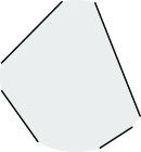
(a) A $2$-dimensional gasket.

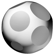
(b) A $3$-dimensional gasket.

Figure 1. Linear gaskets.

We adopt Felix Klein’s projective model of hyperbolic space; in it, $\mathbb{H}^{m}$ is the open unit ball in $\mathbb{R}^{m}$, and each codimension 1 hyperbolic hyperplane is by definition a nonempty intersection with $\mathbb{H}^{m}$ of an affine linear $(m-1)$-plane in $\mathbb{R}^{m}$. A gasket is by definition any oriented cat $m$-manifold that is degree +1 cat isomorphic to a linear gasket.

Remark 2.1.

A linear gasket is clearly simultaneously an oriented manifold of all three categories. The hyperbolic structure of $\mathbb{H}^{m}$ will occasionally be helpful. However it can be treacherous for pl, since its isometries are not all pl; they are projective linear but mostly not affine linear (not even piecewise). Thus our mainstay will be the cat structures inherited from $\mathbb{R}^{m}$.

Consider an indexed set $\mu_{i}=(M_{i},P_{i})$ of CSI pairs of dimension $m$, where $i$ ranges over a nonempty finite or countable index set $S$. The CSI operation yields a CSI pair $\omega=(W,Q)$ by the following construction (see Figure2).

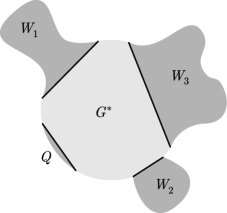
Figure 2. CSI operation.

Let $G^{\ast}$ be a linear gasket of the same dimension $m$, with $\left|S\right|+1$ boundary components. Each closed component of the complement of $G^{\ast}$ in $\mathbb{H}^{m}$ is a cat flange. We choose one, say $Q$, and write $G$ for the gasket $G^{\ast}\cup Q$. The flange $Q$ will become the flange of $\omega$.

A pair that is cat isomorphic to $(G,Q):=(G^{\ast}\cup Q,Q)$ as above will be called a flanged gasket. Equivalently, any CSI pair $(G^{\prime},Q^{\prime})$ where $G^{\prime}$ and $G^{\prime}-{\textnormal{Int}}{Q^{\prime}}$ are both cat gaskets is by definition a flanged gasket.

$W$ will now be formed by introducing identifications in the disjoint sum:

(†) $$\bigsqcup\left\{M_{i}\mid i\in S\right\}\ \sqcup\ G.$$

We index by $S$ the $\left|S\right|$ components of $\partial{G}$, denoting them by $H_{i}$, $i\in S$, and choose, for each, a cat degree +1 embedding $\theta_{i}:P_{i}\to G^{\ast}$ onto an open collar neighborhood of $H_{i}$ in $G^{\ast}$. Now form $W$ from the disjoint sum(† ‣ 2) by identifying $P_{i}$ to its image in $G^{\ast}$ under $\theta_{i}$. Finally, $\omega:=(W,Q)$ is by definition a CSI sum of the CSI pairs $\mu_{i}$, $i\in S$.

We will call $G$ and $G^{\ast}$ respectively the coarse gasket and the fine gasket of the CSI sum $\omega=(W,Q)$.

Remark 2.2.

As a topological space, $W$ is somewhat more simply expressed as the quotient space of the disjoint sum

$$\bigsqcup\left\{M_{i}-{\textnormal{Int}}{P_{i}}\mid i\in S\right\}\ \sqcup\ G$$

by the identifications

$$\theta_{i}|_{\partial{P_{i}}}:\partial{P_{i}}\to H_{i}.$$

In the pl category, these identifications induce a unique pl manifold structure on $W$. But in the diff category, the full collarings $\theta_{i}$ serve to provide a well defined differentiable manifold structure on $W$.

Theorem 2.3.

The CSI of a nonempty but countable (or finite) set of CSI pairs of dimension $m\geq 3$ enjoys the following properties:

(1) From such a set $(M_{i},P_{i})$, $i\in S$, the CSI construction above yields a CSI pair $(W,Q)$ that is well defined up to cat isomorphism. Given a second such construction whose entries are distinguished by primes, a bijection $\varphi:S\to S^{\prime}$, and, for each $i\in S$, an isomorphism of cat CSI pairs $\psi_{i}:(M_{i},P_{i})\to(M^{\prime}_{\varphi(i)},P^{\prime}_{\varphi(i)})$, there exists a cat isomorphism $\psi:(W,G,Q)\to(W^{\prime},G^{\prime},Q^{\prime})$ that extends $\psi_{i}$ restricted to $M_{i}-{\textnormal{Int}}P_{i}$ for all $i\in S$. Furthermore, this $\psi$ is degree $+1$ as a map $G\to G^{\prime}$, and induces an isomorphism of CSI pairs $(W,Q)\to(W^{\prime},Q^{\prime})$. Thus, in addition to being well defined, the CSI operation is commutative.

(2) The composite CSI operation is associative.

(3) The CSI operation has an identity element $\varepsilon=(\mathbb{R}^{m},\mathbb{R}^{m}_{+})$, and the infinite CSI product $\varepsilon\varepsilon\varepsilon\cdots$ of copies of $\varepsilon$ is isomorphic to $\varepsilon$.

Precise definitions of composite CSI operations and of their associativity are given below in Section5.

Notation 2.4.

Theorem2.3 justifies the following notations for CSI sums. If $\mathcal{M}$ is a nonempty but countable collection of flanged manifolds, then ${\textnormal{CSI}}(\mathcal{M})$ can denote the flanged manifold resulting from the CSI operation applied to these manifolds. And, in case $\mathcal{M}$ is an ordered sequence $M_{1}$, $M_{2}$, $\ldots$, then ${\textnormal{CSI}}(M_{1},M_{2},\ldots)$ and ${\textnormal{CSI}}(\mathcal{M})$ should be synonymous. An alternative to ${\textnormal{CSI}}(M_{1},M_{2},...)$ introduced by Gompf[Gom85] is $M_{1}\mathbin{\natural}M_{2}\mathbin{\natural}\cdots$.

Remark 2.5.

In Theorem2.3, it is already striking that every infinite CSI product yields a well defined CSI pair (up to isomorphism). Nothing so strong is true for CS or CSB unless artificial limitations are imposed on the infinite connected sum operation. For example, in dimensions $m\geq 2$, an infinite CS of any closed, connected, oriented $m$-manifold with itself could reasonably be defined so as to have any conceivable end space – to wit any nonempty compact subset of the Cantor set.

Remark 2.6.

For cat = diff and pl, as observed in remarks at the beginning of this section, the interior of a cat compact $m$-manifold with nonempty connected boundary, has a privileged choice of flange (up to ambient isotopy and orientation reversal). This lets us perceive some near overlap of CSI with the ordinary connected sum CS as follows. Let us suppose $M$ is the connected sum $M_{1}\mathbin{\sharp}M_{2}\mathbin{\sharp}\cdots\mathbin{\sharp}M_{k}$ of a finite collection $M_{1},\ldots,M_{k}$ of oriented connected closed $m$-manifolds, then $M-(\textnormal{point})$ is cat isomorphic, preserving orientation, to the flanged and oriented manifold $M^{\prime}_{1}\mathbin{\natural}M^{\prime}_{2}\mathbin{\natural}\cdots\mathbin{\natural}M^{\prime}_{k}$ where $M^{\prime}_{i}$ is the manifold $M_{i}-(\textnormal{point})$ with a flange chosen whose orientation agrees with that of $M_{i}$. The reader is left to further explore such relations between CSI and CS.

Remark 2.7.

The last remark above leads us to simple examples where reversal of a flange orientation changes the underlying proper homotopy type of the CSI of two flanged manifolds.

It is a familiar fact that, if $M$ is the complex projective plane (of real dimension $4$), the ordinary connected sum $M\mathbin{\sharp}(-M)$ has a signature zero cup product bilinear form on the cohomology group

$$\mathrm{H}^{2}(M\mathbin{\sharp}(-M)\,;\,{\mathbb{Z}})={\mathbb{Z}}^{2},$$

whilst $M\mathbin{\sharp}M$ has form of signature $+2$ (the sign $+$ becoming $-$ if we replace $M$ by $-M$). It follows that $M\mathbin{\sharp}M$ and $M\mathbin{\sharp}-M$ are not homotopy equivalent.

Let $N$ be $M-\hbox{(point)}$, the complement of a point in $M$, and forget the orientation of $N$, but then consider two flanges $P_{+}$ and $P_{-}$ for $N$ whose orientations agree with those of $M$ and $-M$ respectively. By Remark2.6, the CSI of $(N,P_{+})$ and $(N,P_{-})$ is $(M\mathbin{\sharp}-M)-\hbox{(point)})$ whose Alexandroff one-point compactification is $(M\mathbin{\sharp}-M)$. On the other hand, the CSI of $(N,P_{+})$ and $(N,P_{+})$ is $(M\mathbin{\sharp}M)-\hbox{(point)})$ whose one-point compactification is $(M\mathbin{\sharp}M)$. There cannot be a proper homotopy equivalence between

$$(M\mathbin{\sharp}-M)-\hbox{(point)}\quad\hbox{and}\quad(M\mathbin{\sharp}M)-\hbox{(point)}$$

because its one-point compactification would clearly be a homotopy equivalence between $M\mathbin{\sharp}-M$ and $M\mathbin{\sharp}M$, which does not exist.

The proof of Theorem2.3 will be mostly elementary. There is one important exception: the top version as presently stated requires the difficult Stable Homeomorphism Theorem (=SHT) of[Kir69, FQ90, Edw84] to show that any homeomorphism of $\mathbb{R}^{m-1}$ is isotopic to a linear map. In contrast, for cat=pl or cat=diff, it is elementary that every cat automorphism of euclidean space is cat isotopic to a linear map (for pl see[RS72], and for diff see[Mil97, p.34]).

Happily, this dependence on a difficult result can and will be removed. Our tactic is to refine the definition of CSI for top requiring henceforth (unless the contrary is indicated) that:

$\bullet$ The CSI flange $P$ in each CSI pair $(M,P)$ shall carry a preferred diff structure making $P$ diff isomorphic to $\mathbb{R}^{m}_{+}$, and, with respect to such structures, every CSI pair isomorphism shall be diff on the flanges.

$\bullet$ Every gasket shall be equipped with a diff structure making it diff isomorphic to a linear gasket, and all of the identifications made in CSI constructions shall be diff identifications with respect to these preferred diff structures.

The magical effect of this refined definition is that the proof for diff of the basic properties of CSI applies without essential changes to the top category. This is rather obvious if one thinks of top CSI as being diff where all of the relevant action takes place. Consequently, for many cases of Theorem2.3 we give little or no proof for the top category – leaving the reader to do his own soul searching. Note that the above refinement could equally use pl in place of diff.

3. Regular Neighborhoods

Regular neighborhoods will play a central technical role throughout this article. A short discussion of such cat neighborhoods, just sufficient for our uses, is given below.

PL Regular Neighborhoods.

pl regular neighborhood theory is a major feature of pl topology that is entirely elementary but not always simple. Such a theory was first formulated by J.H.C.Whitehead [Whi39], and then simplified and improved by E.C.Zeeman[Zee63, HZ64] (see also[RS72]). We need the version of this theory that applies to possibly noncompact pl spaces; it is developed in[Sco67]. We now review some key facts.

Let $X$ be a closed pl subspace of the pl space $M$. Neither is assumed to be compact, connected, nor even a pl manifold. Recall that $X$ is a subcomplex of some pl triangulation of $M$ by a locally finite simplicial complex. A regular neighborhood $N$ of $X$ can be defined to be a closed $\varepsilon$-neighborhood ($\varepsilon<0.5$) of $X$ in $M$ for the barycentric metric of some such triangulation of $M$. The frontier of $N$ in $M$ is thus pl bicollared in $M$.

We quickly recite some familiar facts. Any two regular neighborhoods $N$ and $N^{\prime}$ of $X$ in $M$ are ambient isotopic fixing $X$. If $N_{0}$ is a regular neighborhood that lies in the (topological) interior ${\textnormal{int}}\,N$ of $N$ in $M$, then the triad $(N-{\textnormal{int}}\,N_{0};\delta N_{0},\delta N)$ is pl isomorphic to the product triad $\delta N\times([0,1];0,1)$ where $\delta$ indicates frontier in $M$. Thus, if $N_{0}$ is contained in ${\textnormal{int}}\,N\cap{\textnormal{int}}\,N^{\prime}$, and $U$ is a neighborhood of $N\cup N^{\prime}$ in $M$, then the ambient isotopy carrying $N$ to $N^{\prime}$ can be the identity on $N_{0}$ and on the complement of $U$.

We will also use (in some special cases) two less familiar facts, namely Propositions3.1 and3.2.

Proposition 3.1.

If $N_{i}$ is a regular neighborhood of $X_{i}$ in $M_{i}$ for $i=1$ and $i=2$, then $N_{1}\times N_{2}$ is a regular neighborhood of $X_{1}\times X_{2}$ in $M_{1}\times M_{2}$. ∎

Proposition 3.2.

Let $N$ be a properly embedded $m$-submanifold of a pl $m$-manifold $M$ such that $N\subset{\textnormal{Int}}\,M$, and let $X$ be a properly embedded pl subspace of $M$ with $X\subset N$. Then a sufficient condition for $N$ to be a regular neighborhood of $X$ in $M$ is that $(N,X)$ be pl isomorphic to a pair $(N^{\prime},X^{\prime})$ where $N^{\prime}$ is a regular neighborhood of $X^{\prime}$ in a pl manifold $M^{\prime}$. ∎

Proposition 3.3.

If $\rho:[0,\infty)\to\mathbb{R}^{m}_{+}$ is a proper linear ray embedding with image $r$ in ${\textnormal{Int}}\,\mathbb{R}^{m}_{+}$, then $\mathbb{R}_{+}^{m}$ is pl isomorphic fixing $r$ to a regular neighborhood of $r$ in $\mathbb{R}^{m}_{+}$.

Proof of Proposition3.3 from Propositions3.1 and3.2.

Adjusting $r$ by an affine linear automorphism of $\mathbb{R}_{+}^{m}$, we may assume, without loss of generality, that $r=0\times[2,\infty)$, where the $0$ here denotes the origin of $\mathbb{R}^{m-1}=\partial{\mathbb{R}_{+}^{m}}$.

For any real $\lambda>0$ and integer $k>0$, let $B_{\lambda}^{k}:=[-\lambda,\lambda]^{k}$ and let $B_{<\lambda}^{k}:=(-\lambda,\lambda)^{k}$. Since each $B_{\lambda}^{m-1}$ is a regular neighborhood of the origin, there exists a pl isomorphism for any $\varepsilon\in(0,1)$:

$$\varphi:\mathbb{R}^{m-1}-B_{<\varepsilon}^{m-1}\to[\varepsilon,\infty)\times\partial{B_{\varepsilon}^{m-1}}$$

extending the canonical identification $\partial{B_{\varepsilon}^{m-1}}\cong\varepsilon\times\partial{B_{\varepsilon}^{m-1}}$. Although $\varphi$ itself is not canonical, we regard it as an identification.

By Proposition3.1, the product $B_{1}^{m-1}\times[1,\infty)$ is a regular neighborhood of $r$ in $\mathbb{R}_{+}^{m}$. Thus, by Proposition3.2, it certainly will suffice to show that there exists, for some $\varepsilon\in(0,1)$, a pl isomorphism

$$h:\mathbb{R}^{m-1}\times[1,\infty)\to B_{1}^{m-1}\times[1,\infty)$$

fixing $B_{\varepsilon}^{m-1}\times[2,\infty)$.

For $\varepsilon\in(0,1)$, it is an elementary fact about pl $2$-manifolds that there is a pl isomorphism:

$$\theta:[\varepsilon,\infty)\times[1,\infty)\to[\varepsilon,1]\times[1,\infty)$$

fixing $\varepsilon\times[1,\infty)$. Producting with the identity map of $\partial{B_{\varepsilon}^{m-1}}$, and then extending by the identity over $B_{\varepsilon}^{m-1}\times[1,\infty)$, we get the required pl isomorphism $h$ for (†). ∎

DIFF Regular Neighborhoods.

There is a quite general elementary theory of smooth regular neighborhoods in diff manifolds. Unfortunately, it involves pl, is fastidious to develop, and currently occupies half of the monograph[HM74] (see also[Cai67]). We therefore cobble together an ad hoc, but bootstrapping, notion of diff regular neighborhood for a diff ray $r$ in a diff $m$-manifold $M$ ($r$ is a proper diff embedded copy of $[0,\infty)$ in $M$). This notion will be derived from the well known notion of a tube about a submanifold and can be extended to most sorts of diff submanifolds.

Let $p:V(r)\to r$ be the projection of a diff tube about the ray $r$. $V(r)$ is a diff submanifold of $M$ lying in $\text{Int}M$. It is a trivial diff bundle with projection $p$, fiber the unit $(m-1)$-disk, orthogonal group, and zero section the inclusion of $r$. It is not, however, a neighborhood of ${\partial}r=b$, nor a neighborhood of r itself. Also $V(r)$ has undesirable corners. To obtain an acceptable regular neighborhood of $r$, we trim $V(r)$ and add a cap along the butt end $p^{-1}(b)$ as follows (see Figure3).

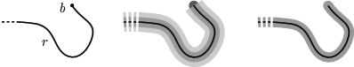
Figure 3. A diff regular neighborhood of a ray. The light gray (in center figure) indicates a tube about the ray $r$, and the dark gray (center and right) indicates the regular neighborhood of $r$.

Let $V^{\prime}(r)\subset V(r)$ be the subbundle of disks of radius $1/2$. In the diff manifold with boundary (and corners) $M_{0}=M-\text{Int}V(r)$, the point $b={\partial}r$ is a boundary point and the disk fiber $E^{m-1}$ of $V^{\prime}$ at $b$ is a tube about $b$ in ${\partial}M_{0}$. There exists a tubular neighborhood $U(b)$ of $b$ in $M_{0}$. By diff tube uniqueness, we can arrange that $U(b)\cap{\partial}M_{0}$ coincides with $E^{m-1}$. Further, applying diff collaring existence and uniqueness to ${\partial}M_{0}$ in $M$, we can arrange that $T(r)=V^{\prime}(r)\cup U(b)$ is smooth along ${\partial}E^{m-1}$, and hence is a diff submanifold of $M$ without corners. This $T(r)$ is, by definition, a diff regular neighborhood of $r$ in $M$.

For a (proper) diff submanifold $L$, each component of which is a diff ray, we further define a diff regular neighborhood to be a diff codimension$0$ submanifold that is a disjoint union of regular neighborhoods of the component rays of $L$.

Ambient diff isotopy uniqueness of tubes and collars readily establishes ambient diff isotopy uniqueness of such diff regular neighborhoods. With some care, the isotopy can be kept fixed outside any open neighborhood of the union of two such regular neighborhoods.

Observe that this definition makes it easy to see that $\mathbb{R}^{m}_{+}$ is a diff regular neighborhood of any affine linear ray in $\mathbb{R}^{m}$ that lies in the interior of $\mathbb{R}^{m}_{+}$. Indeed, the corresponding tube about $r$ can have spherical caps as fibers as shown in Figure4. Note that Proposition3.3 above is the pl analogue of this fact.

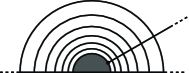
Figure 4. $\mathbb{R}^{m}_{+}$ is a diff regular neighborhood of an affine linear ray.

TOP Open Regular Neighborhoods.

There is no simple elementary theory of closed top regular neighborhoods. This deficiency will be overcome using a simple elementary notion of open regular neighborhood that is adequate for proving the Cantrell-Stallings hyperplane unknotting theorem for top using CSI. Incidentally, such open regular neighborhoods could serve in proving the pl and diff versions of the hyperplane unknotting theorem, in lieu of the more precise closed cat regular neighborhood theory.

Let $W$, $X$, $Y$ and $Z$ be locally compact (but not necessarily compact!) metrizable spaces, where $Z$ is a closed subset of $W$. Consider a proper continuous surjection $f:X\to Z$ and define the infinite radius mapping cylinder $\text{Map}(f)$ to be the quotient of the disjoint union $X\times[0,\infty)\sqcup Z$ by the relation that identifies $(x,0)$ to $f(x)\in Z$ for all $x\in X$. Clearly, $Z$ is closed in $\text{Map}(f)$ and the open subset $X\times(0,\infty)$ is its complement. For $\rho>0$, we define the radius $\rho$ mapping cylinder $\text{Map}_{\rho}(f)$ to be the quotient of $X\times[0,\rho]\sqcup Z$ in $\text{Map}(f)$ and also the open one $\text{Map}_{<\rho}(f)$ to be the quotient of $X\times[0,\rho)\sqcup Z$ in $\text{Map}(f)$.

Let $g:Y\to Z$ be another such map (same target, but different source). Suppose that $\text{Map}(f)$ and $\text{Map}(g)$ are embedded, fixing $Z$, as open neighborhoods of $Z$ in $W$. Then, we have the following well known result, where $A\Subset B$ for sets in a space $W$ means that the closure of $A$ in $W$ is contained in the interior of $B$ in $W$.

Theorem 3.4 (Open Mapping Cylinder Neighborhood Uniqueness).

If $\textnormal{Map}_{1}(f)\Subset\textnormal{Map}(g)$, then there exists a homeomorphism of $\textnormal{Map}(f)$ onto $\textnormal{Map}(g)$ that fixes pointwise $\textnormal{Map}_{1}(f)$. Consequently

$$\textnormal{Map}(g)-\textnormal{Map}_{<1}(f)$$

is homeomorphic to $X\times[1,\infty)$ fixing $X\times 1$.

Remarks 3.5.

(1) Although $\textnormal{Map}_{1}(f)$ is clearly closed in $\textnormal{Map}(f)$, the conclusion of the theorem is false if $\textnormal{Map}_{1}(f)$ is not closed in $\textnormal{Map}(g)$, and this may occur even when $\textnormal{Map}(f)\subset\textnormal{Map}(g)$ as shown in Figure5.

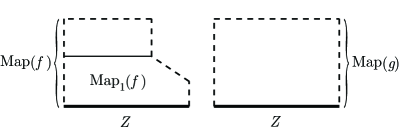
Figure 5. Example where $\textnormal{Map}(f)\subset\textnormal{Map}(g)$, but $\textnormal{Map}_{1}(f)$ is not closed in $\textnormal{Map}(g)$ and hence is not closed in any space $W$ containing $\textnormal{Map}(g)$. Here, $\textnormal{Map}(g)={(0,1)\times[0,\infty)}$, $Z={(0,1)\times 0}$, and ${X=(0,1)}$.

On the other hand, there then always exists a self-homeomorphism $h$ of $\textnormal{Map}(f)$ such that $h(\textnormal{Map}_{1}(f))$ is closed in $W$.

(2) Even when $X$ and $Y$ are both top manifolds, the conclusion of this theorem does not imply that $X$ is homeomorphic to $Y$. Further, if they happen to be homeomorphic, $X\times 1$ is not in general ambient isotopic to $Y\times 1$ (see[Mil61] and the top invariance of simple homotopy type in[KS69], and Essay III of[KS77]).

(3) Theorem3.4 remains true if $X$, $Y$, and $Z$ are merely Hausdorff and paracompact[SGH73, p.260], but we do not need this generality.

Proof.

The most appropriate proof to recall here is one using an infinite composition trick that is often called the ‘Eilenberg-Mazur swindle’ (see also[Sta62, Sta65]). Without loss we may assume that $W=\textnormal{Map}(g)$. After reembedding $\text{Map}(f)$ and $\text{Map}(g)$ into $W$ by suitable topological automorphisms of $\text{Map}(f)$ and $\text{Map}(g)$ respectively, with their supports disjoint from $\textnormal{Map}_{1}(f)$, we can assume that radius 1 and radius 2 mapping cylinders are shuffled as follows

(*) $$\text{Map}_{1}(f)\Subset\text{Map}_{1}(g)\Subset\text{Map}_{2}(f)\Subset\text{Map}_{2}(g).$$

Here one uses the local compactness and metrizability hypotheses (see[KR63]).

The triad $\gamma=(V;X\times 1,Y\times 1)$, where $V$ is $\text{Map}_{1}(g)$ minus the topological interior of $\text{Map}_{1}(f)$, can be regarded as a cobordism from $X$ to $Y$ (see[Mil65]).

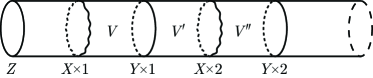
Figure 6. Shuffled mapping cylinders.

The relations (* ‣ Proof) show that $\gamma$ has an inverse $\gamma^{\prime}=(V^{\prime};Y\times 1,X\times 2)$ viewed as a cobordism from $Y$ to $X$, where $V^{\prime}$ is $\text{Map}_{2}(f)$ minus the topological interior of $\text{Map}_{1}(g)$ (see Figure6). In other words, the end to end cobordism composition $\gamma\cdot\gamma^{\prime}$ is topologically the product cobordism $\varepsilon_{X}$ on $X$, written $\gamma\cdot\gamma^{\prime}\cong\varepsilon_{X}$. Similarly, $\gamma^{\prime}$ has an inverse $\gamma^{\prime\prime}=(V^{\prime\prime};X\times 2,Y\times 2)$, where $V^{\prime\prime}$ is $\text{Map}_{2}(g)$ minus the topological interior of $\text{Map}_{2}(f)$, written $\gamma^{\prime}\cdot\gamma^{\prime\prime}\cong\varepsilon_{Y}$. Using an obvious associativity, we see that $\gamma$ and $\gamma^{\prime\prime}$ are isomorphic cobordisms

$$\gamma\cong\gamma\cdot\varepsilon_{Y}\cong\gamma\cdot(\gamma^{\prime}\cdot\gamma^{\prime\prime})\cong(\gamma\cdot\gamma^{\prime})\cdot\gamma^{\prime\prime}\cong\varepsilon_{X}\cdot\gamma^{\prime\prime}\cong\gamma^{\prime\prime}.$$

In particular, $\gamma^{\prime}\cdot\gamma\cong\varepsilon_{Y}$.

$\text{Map}(f)$ minus the interior of $\text{Map}_{1}(f)$ is (the body of) the infinite cobordism composition $\varepsilon_{X}\cdot\varepsilon_{X}\cdot\varepsilon_{X}\cdots$, while $\text{Map}(g)$ minus the interior of $\text{Map}_{1}(f)$ is the infinite composition $\gamma\cdot\varepsilon_{Y}\cdot\varepsilon_{Y}\cdot\varepsilon_{Y}\cdots$. But, these are the same by the infinite product swindle, again using associativity

$$\gamma\cdot\varepsilon_{Y}\cdot\varepsilon_{Y}\cdot\varepsilon_{Y}\cdots \cong\gamma\cdot(\gamma^{\prime}\cdot\gamma)\cdot(\gamma^{\prime}\cdot\gamma)\cdot(\gamma^{\prime}\cdot\gamma)\cdots$$

$$\cong(\gamma\cdot\gamma^{\prime})\cdot(\gamma\cdot\gamma^{\prime})\cdot(\gamma\cdot\gamma^{\prime})\cdots$$

$$\cong\varepsilon_{X}\cdot\varepsilon_{X}\cdot\varepsilon_{X}\cdots.\hskip 126.0pt\qed$$

4. Radial Ray and Linear Gasket Uniqueness

In this section, cat will mean either pl or diff. We begin with a ray unknotting lemma for radial rays in $\mathbb{H}^{m}$. Let $L\cong\mathbb{Z}_{+}\times[0,\infty)$ be a proper cat embedded submanifold of $\mathbb{H}^{m}$ so that all rays $r_{i}=i\times[0,\infty)$ are radial, i.e. each ray is contained in a line through the origin in $\mathbb{R}^{m}\supset\mathbb{H}^{m}$, and is disjoint from the origin. In what follows, lengths come from the standard euclidean metric on $\mathbb{R}^{m}$. For each $i\in\mathbb{Z}_{+}$, let $d_{i}$ denote the distance from the origin in $\mathbb{R}^{m}$ to the initial point of $r_{i}$ parameterized by $i\times 0$, and let $p_{i}$ denote the limit point of $r_{i}$ in $S^{m-1}={\partial}\overline{\mathbb{H}}^{m}$, where $\overline{\mathbb{H}}^{m}$ is the unit ball $B^{m}$ that is the closure of $\mathbb{H}^{m}$ in $\mathbb{R}^{m}$.

Let $L^{\prime}$ be another such submanifold, and define $r^{\prime}_{i}$, $d^{\prime}_{i}$, and $p^{\prime}_{i}$ in the same way. Also, let $f:L\to L^{\prime}$ be a cat isomorphism. Notice that both sequences $d_{i}$ and $d^{\prime}_{i}$ converge to 1 as $i\to\infty$ since $L$ and $L^{\prime}$ are properly embedded.

$S(t_{1},t_{2})$, with $0<t_{1}<t_{2}\leq 1$, will denote the thickened sphere of points $x\in\mathbb{H}^{m}$ such that $t_{1}\leq\|x\|\leq t_{2}$.

Lemma 4.1 (Radial Ray Uniqueness).

With the above data, suppose $m\geq 3$. Then there is a cat ambient isotopy $h_{t}$ of $\mathbb{H}^{m}$, $0\leq t\leq 1$, such that $h_{0}$ is the identity and $h_{1}|_{L}=f$.

Remark 4.2.

This ambient isotopy of $\mathbb{H}^{m}$ cannot in general extend to an ambient isotopy of the ball $\overline{\mathbb{H}}^{m}$ since the accumulation points in ${\partial}\overline{\mathbb{H}}^{m}$ of $L$ would then be homeomorphic to those of $L^{\prime}$. On the other hand, $p_{i}$ can be an arbitrary sequence of distinct points in ${\partial}\overline{\mathbb{H}}^{m}$; thus its set of accumulation points in ${\partial}\overline{\mathbb{H}}^{m}$ may be any nonempty compact subset.

Proof of Lemma 4.1 for diff.

Reindex the rays $r_{i}$ so that $f(r_{i})=r^{\prime}_{i}$. Since any diff automorphism of $[0,\infty)$ is isotopic to the identity, it will suffice to construct $h_{t}$ as above so that $h_{1}(r_{i})=r^{\prime}_{i}$. Reindexing rays, we can assume that $d_{i}\leq d_{i+1}$ for $i\in\mathbb{Z}_{+}$. It is elementary that $d_{i}\to 1$ as $i\to\infty$.

A preliminary ambient isotopy sets the stage. Shrink the rays $r_{i}$ radially towards their limit points $p_{i}$ so that $d_{i}\geq d^{\prime}_{i}$ (while maintaining $d_{i}\leq d_{i+1}$). This is straightforward using a regular neighborhood of $L$ in $\mathbb{H}^{m}$.

Now, choose a diff simple path $\alpha_{1}$ in $S^{m-1}$ from $p_{1}$ to $p^{\prime}_{1}$. This path obviously permits construction of an isotopy of $S^{m-1}$ supported near the path and taking $p_{1}$ to $p^{\prime}_{1}$. Extending this isotopy radially gives an ambient isotopy of $S(d_{1},1)$ taking the ray $r_{1}$ to a subset of $r^{\prime}_{1}$ (recall, we arranged that $d_{i}\geq d^{\prime}_{i}$). This ambient isotopy of $S(d_{1},1)$ extends naturally to one of $\overline{\mathbb{H}}^{m}$ fixing the ball of radius $d_{1}-\varepsilon_{1}$ for any small $\varepsilon_{1}>0$. At the end of this isotopy, any ray $r_{i}$, $i\geq 2$, that moved has image another radial ray of the same length which (abusing language) we still refer to as $r_{i}$ with endpoint $p_{i}$.

Next, similarly form an isotopy of $S^{m-1}$ moving $p_{2}$ to $p^{\prime}_{2}$ and having support missing $p^{\prime}_{1}$. Extending radially to $S(d_{2},1)$ we get an ambient isotopy (fixing $r^{\prime}_{1}\supset r_{1}$) taking $r_{2}$ to a subset of $r^{\prime}_{2}$.

Inductively form an isotopy of $S^{m-1}$ moving $p_{i}$ to $p^{\prime}_{i}$ and with support disjoint from $p^{\prime}_{j}$, for $1\leq j\leq i-1$. Extend as before to get an ambient isotopy of $\overline{\mathbb{H}}^{m}$ with support in $S(d_{i}-\varepsilon_{i},1)$ taking $r_{i}$ to a subset of $r^{\prime}_{i}$ while fixing $r^{\prime}_{j}\supset r_{j}$, for $1\leq j\leq i-1$. Here, $\varepsilon_{i}$ lies in $(0,d_{i})$ and $\varepsilon_{i}\to 0$ as $i\to\infty$. Also, since $d_{i}\to 1$ as $i\to\infty$, the points in any compact set in $\mathbb{H}^{m}$ are moved at most finitely many times. Hence, the time interval composition of all of these ambient isotopies provides a well defined ambient isotopy of $\mathbb{H}^{m}$ (but usually not one of $\overline{\mathbb{H}}^{m}$). We now have $r_{i}\subset r^{\prime}_{i}$ for all $i\in\mathbb{Z}_{+}$. A final ambient isotopy stretches each $r_{i}$ so that $d_{i}=d^{\prime}_{i}$, finishing the proof for diff. ∎

Proof of Lemma 4.1 for pl.

Make a preliminary pl identification $\Theta$ of the thickened standard pl $(m-1)$-sphere $\Sigma^{m-1}\times(0,1)$ to the complement of the origin $\mathbb{H}^{m}-0$ in such a way that each component of $L$ and of $L^{\prime}$ lies in a modified ray

$$\Theta\left((\textnormal{point})\times(0,1)\right)\subset\Theta\left(\Sigma^{m-1}\times(0,1)\right)=\mathbb{H}^{m}-0.$$

Now, imitate the diff proof. ∎

Remark 4.3.

There is no such pl identification $\Theta$ that sends every ray of the form $\left((\textnormal{point})\times(0,1)\right)\subset\Sigma^{m-1}\times(0,1)$ to a radial ray in $\mathbb{H}^{m}-0$, not even when $m=2$. This is a corollary of the observation that the point preimages under any linear surjection $\mathbb{R}^{m}\to\mathbb{R}^{m-1}$ are the set of all lines in $\mathbb{R}^{m}$ parallel to the kernel line. Thus, the construction of $\Theta$ must be adapted to $L$ and $L^{\prime}$, for example by using a well chosen triangulation in which $L$ and $L^{\prime}$ are $1$-subcomplexes.

Combined with pl and diff regular neighborhood theory (see Section3), the above radial ray uniqueness lemma (Lemma4.1) will let us prove a linear gasket uniqueness lemma that we now formulate. Adopting the context and terminology established for Lemma4.1, fix a category cat to be pl or diff. Let $G$ be a linear gasket of dimension $m\geq 3$; i.e., a submanifold of $\mathbb{H}^{m}$ bounded by countably many disjoint hyperbolic hyperplanes $H_{i}$, $i\in\mathbb{Z}_{+}$. Let $G^{\prime}$ be another such gasket of dimension $m$ and distinguish corresponding subsets by primes.

Lemma 4.4 (Linear Gasket Uniqueness).

Given the data above, there is a cat ambient isotopy $g_{t}$ of $\mathbb{H}^{m}$, $0\leq t\leq 1$, so that $g_{0}=\textnormal{id}|_{\mathbb{H}^{m}}$, $g_{1}(G)=G^{\prime}$, and $g_{1}(H_{i})=H^{\prime}_{i}$ for all $i\in\mathbb{Z}_{+}$.

Corollary 4.5.

If $G$ and $G^{\prime}$ are gaskets and $f:{\partial}G\to{\partial}G^{\prime}$ is a degree $+1$ cat isomorphism of their boundaries, then $f$ extends to a cat isomorphism $F:G\to G^{\prime}$. ∎

Proof of Lemma 4.4.

Without loss of generality, we assume that $G$ and $G^{\prime}$ are linear gaskets in $\mathbb{H}^{m}$. The gasket $G$ determines a canonical cat submanifold $L\cong\mathbb{Z}_{+}\times[0,\infty)$ of $\mathbb{H}^{m}$ as follows: each hyperplane boundary component $H_{i}$, $i\in\mathbb{Z}_{+}$, of the gasket $G$ defines a proper radial ray $r_{i}$ in $\mathbb{H}^{m}$, namely the one orthogonal to $H_{i}$, having endpoint the point of $H_{i}$ closest to the origin in $\mathbb{R}^{m}$, and extending outwards from $G$. The union of these rays is defined to be $L$. For each $H_{i}$, let $V_{i}$ denote the closed complementary component of $\mathbb{H}^{m}-\text{Int}G$ with boundary $H_{i}$. If $r$ is any radial ray in $\mathbb{H}^{m}$, then let $s$ denote the radial ray obtained from $r$ by shrinking it outwards radially to be half as long (for the euclidean metric). Each $V_{i}$ is isomorphic to the closed upper half space $\mathbb{R}^{m}_{+}$ and is a cat regular neighborhood of $s_{i}$ as we have observed in Section3. Similarly, the gasket $G^{\prime}$ canonically determines closed complementary components $V^{\prime}_{i}$, rays $r^{\prime}_{i}$, and shortened rays $s^{\prime}_{i}$.

After a preliminary isotopy provided by Lemma4.1 (radial rayuniqueness), we may assume $r_{i}=r^{\prime}_{i}$ for all $i\in\mathbb{Z}_{+}$, and hence $s_{i}=s^{\prime}_{i}$ for all $i\in\mathbb{Z}_{+}$. By cat regular neighborhood ambient uniqueness, we may now ambiently isotop $V_{i}$ to $V^{\prime}_{i}$ for all $i$ (simultaneously), completing the proof. ∎

Remark 4.6.

Lemmas4.1 and4.4 hold also for a finite index set in place of $\mathbb{Z}_{+}$. One can deduce this from the case of $\mathbb{Z}_{+}$. Or, one can note that the same proofs apply.

Remark 4.7.

As it is stated, Lemma4.1 (radial ray uniqueness) fails in dimension $2$, even for three rays. Any set of distinct radial rays in $\mathbb{H}^{2}$ obviously inherits a natural cyclic order from that of their limit points on the circle $S^{1}$. The proof of Lemma4.1 actually shows that such a collection of rays is determined up to ambient isotopy of $\mathbb{H}^{2}$ by the isomorphism class of its cyclic ordering. There are many such classes when the number of rays is infinite. For example, the number of rays with no immediate successor (or predecessor) is then an invariant. In fact, there are uncountably many such classes. We are confident that, taking account of this natural ray order, one can nevertheless define an associative CSI operation for 2-manifolds. It is non-commutative in general for 2-manifolds with boundary.

5. Proof of Theorem2.3: Basic Properties of CSI

Proof of Property(1): Well Definition and Commutativity of CSI.

Let cat be pl or diff. Recall that with the data introduced for the statement of Property (1) of Theorem2.3 above, we are seeking a certain sort of cat isomorphism of triples $\psi:(W,G,Q)\to(W^{\prime},G^{\prime},Q^{\prime})$. On the closed complements of the gasket interiors, this $\psi$ is rigidly prescribed by the data; call this $\psi_{0}:W-\text{Int}G\to W^{\prime}-\text{Int}G^{\prime}$. This $\psi_{0}$ has degree $+1$ as a map ${\partial}G\to{\partial}G^{\prime}$. Further, the $\psi$ we seek is prescribed up to isotopy on $Q$ as a degree $+1$ isomorphism $Q\to Q^{\prime}$. Thus, denoting by $H$ and $H^{\prime}$ the fine gaskets $G-\text{Int}Q$ and $G^{\prime}-\text{Int}Q^{\prime}$, it suffices to extend $\psi|:{\partial}H\to{\partial}H^{\prime}$ to a cat degree $+1$ isomorphism $H\to H^{\prime}$ of the fine gaskets. This extension exists by Corollary 4.5. ∎

We explain the notion of a countable indexed set $\mathcal{M}$ of flanged manifolds. It consists of a set $I$ that is finite or countably infinite, and a map of $I$ into the class of flanged $m$-manifolds. The set $I$ is called the index set and, in what follows, will always be a subset of $\mathbb{N}$ or of $\mathbb{N}^{2}$. If we write $\mathcal{M}=\left\{M_{i}\mid i\in I\right\}$, then the flanged manifold corresponding to $i\in I$ is $M_{i}$. It is not always required that $M_{i}$ and $M_{j}$ be disjoint or even distinct when $i\neq j$ in $I$. Thus one can also similarly define an indexed set in any class — in place of the class of flanged manifolds — for example in the class of cat isomorphism classes of flanged manifolds.

Composite CSI Operations and Associativity.

To elucidate associativity, we must make its meaning more precise. Our proof of the Cantrell-Stallings hyperplane unknotting theorem uses only a simple (but infinite) associativity which is expressible in traditional algebraic notation. But, the CSI operation enjoys a natural associativity that is at once more general and equally straightforward to establish. Some tree combinatorics will be involved. More specifically, we introduce what we call a tree of flanged gaskets. The category cat in which we work here is again pl or diff, and the manifold dimension $m$ will be $\geq 3$.

A rooted tree will mean a countable simplicial tree (not necessarily locally finite) that has a distinguished vertex $v_{0}$ called the root. In such a tree, there is a natural orientation of the edges. Indeed, from each vertex $v\neq v_{0}$ there is a unique oriented edge $vv^{\prime}$ joining $v$ to a vertex $v^{\prime}$ strictly nearer to the root vertex in the obvious simplicial path metric.

A tree of $m$-dimensional flanged gaskets is a rooted abstract tree $\mathcal{G}$ whose vertices and edges are given as as follows:

(1) The vertex set of $\mathcal{G}$ is a finite or countable indexed set $\left\{G_{i}\mid i\in I\right\}$ of disjoint $m$-dimensional flanged gaskets. The flange of $G_{i}$ is denoted $F_{i}$ and the root vertex of $\mathcal{G}$ is denoted $G_{0}$. Furthermore, the boundary components of $G_{i}$ are indexed as $H_{i,j}$, $j\in J_{i}$.

(2) There is a unique oriented edge of $\mathcal{G}$ joining any vertex $G_{i}\neq G_{0}$ to the unique adjacent vertex (= flanged gasket) $G_{i^{\prime}}$ that is nearer to $G_{0}$. This edge is presented as an ordered pair $\left(G_{i},H_{i^{\prime},j}\right)$ where, as the notation indicates, $H_{i^{\prime},j}$ is one of the indexed boundary components of $G_{i^{\prime}}$. Each boundary component of the disjoint sum $\left|G\right|=\sqcup_{i}\left|G_{i}\right|$ is required to occur in at most one edge of $\mathcal{G}$.

By the following gluing process, $\mathcal{G}$ determines a cat composite flanged gasket denoted ${\left\|\mathcal{G}\right\|}$. In the disjoint sum $\left|G\right|=\sqcup_{i}\left|G_{i}\right|$, make these identifications: for each edge $\left(G_{i},H_{i^{\prime},j}\right)$ of $\mathcal{G}$, identify the flange $F_{i}$ of $G_{i}$ to a small open collar of $H_{i^{\prime},j}$ in $\left|G_{i^{\prime}}\right|$ by an orientation preserving cat isomorphism $\theta_{i,i^{\prime}}$. Here ‘small’ should mean inside a prescribed open collar neighborhood of the boundary $\partial{(G_{i^{\prime}}-F_{i^{\prime}})}$ of the fine gasket of $G_{i^{\prime}}$, so that the flanges identified into $G_{i^{\prime}}$ obviously do not intersect. Since degree determines $\theta_{i,i^{\prime}}$ up to isotopy, ${\left\|\mathcal{G}\right\|}$ is determined up to cat isomorphism that is the identity outside of an arbitrarily small bicollar neighborhood in ${\left\|\mathcal{G}\right\|}$ of the identified boundary components $\partial{F_{i}}=H_{i^{\prime},j}$.

Lemma 5.1.

With the above definitions, the pair $({\left\|\mathcal{G}\right\|},F_{0})$ is a flanged gasket.

The proof of Lemma5.1 will come after we complete the definition of a composite CSI operation based on $\mathcal{G}$.

For each $i\in I$, consider the set $J^{+}_{i}\subset J_{i}$ of those $j\in J_{i}$ (if any) such that, for no $k\in I$, does there exist an edge $\left(G_{k},H_{i,j}\right)$. By the construction of ${\left\|\mathcal{G}\right\|}$, its boundary $\partial{{\left\|\mathcal{G}\right\|}}$ is a disjoint sum

$$\bigsqcup\left\{H_{i,j}\mid i\in I\textnormal{ and }j\in J^{+}_{i}\right\}.$$

By definition, a composite CSI operation according to the rooted tree $\mathcal{G}$ of flanged gaskets as above involves an indexed set of flanged $m$-manifolds to be ‘summed’

$$\left\{M_{i,j}\mid i\in I\textnormal{ and }j\in J^{+}_{i}\right\}.$$

The corresponding ‘sum’ is the flanged manifold (flanged by $F_{0}$) obtained by gluing the flange of each such $M_{i,j}$ by a degree +1 isomorphism to a small open collar of $H_{i,j}$ in ${\left\|\mathcal{G}\right\|}$ (clearly this open collar may be chosen in $\left|G_{i}\right|$).

Proof of Lemma 5.1.

With the notations established above, it suffices to prove that the flanged manifold ${\left\|\mathcal{G}\right\|}$ is a flanged gasket. This is immediate from the following more primitive lemma (which will be reused in Section9 in our proof of the MHLT (Theorem9.2)). ∎

Lemma 5.2.

For cat=diff or pl, suppose that an oriented cat $m$-manifold $X$ is a finite or countable union of cat gaskets $G_{i}$, $i\in I$, any two of which are either disjoint or intersect in a single boundary component of each. Suppose also that the nerve of the closed cover $\left\{G_{i}\mid i\in I\right\}$ of X is a simplicial tree $\mathcal{T}$. Then $X$ is a cat gasket.

Proof of Lemma 5.2.

Without loss of generality, we assume $I$ is $\mathbb{N}$ or a finite initial segment of $\mathbb{N}$. Reindexing the $G_{i}$, we can arrange that, for all $i\geq 0$, the gasket $G_{i+1}$ is adjacent in $X$ to the connected block

$$X_{i}:=G_{0}\cup G_{1}\cup\cdots\cup G_{i}.$$

By definition, $G_{0}=X_{0}$ can be degree +1 embedded in $\mathbb{H}^{m}$ with frontier made up of hyperbolic hyperplanes.

Suppose inductively that $\phi_{i}:X_{i}\to\mathbb{H}^{m}$ is such an embedding for some $i\geq 0$. Write $X^{\prime}_{i}$ for $\phi_{i}(X_{i})$, write $H_{i}$ for the boundary component of $X_{i}$ that is shared with $G_{i+1}$, and write $H^{\prime}_{i}$ for the hyperbolic hyperplane $\phi_{i}(H_{i})$. We will extend this embedding $\phi_{i}$ to one of $X_{i+1}=X_{i}\cup G_{i+1}$.

Let $Y^{+}_{i}$ be the closed halfspace in $\mathbb{H}^{m}$ bounded by $H^{\prime}_{i}$ that does not intersect ${\textnormal{Int}}{X^{\prime}_{i}}$. In ${\textnormal{Int}}{Y^{+}_{i}}$ choose as many disjoint halfspaces (each bounded by a hyperbolic hyperplane) as $G_{i+1}$ has boundary components disjoint from $X_{i}$; then delete the interiors of those halfspaces from $Y^{+}_{i}$. With the intent to assure that the ultimate embedding of $X$ will be proper, we can and do

• choose these halfspaces within the $1/(i+1)$ neighborhood of the frontier sphere $S^{m-1}$ of $\mathbb{H}^{m}$ in $\mathbb{R}^{m}$ (for the euclidean distance of $\mathbb{R}^{m}$).

The result is a linear gasket $G^{\prime}_{i+1}$ in $\mathbb{H}^{m}$ adjacent to $X^{\prime}_{i}$, more precisely $X^{\prime}_{i}\cap G^{\prime}_{i+1}=H^{\prime}_{i}$. By Corollary4.5 concerning cat uniqueness of linear gaskets, there is a cat isomorphism $G_{i+1}\to G^{\prime}_{i+1}$ agreeing with $\phi_{i}$ on $H_{i}$ and thus extending $\phi_{i}|_{H_{i}}$ to a cat embedding $\psi_{i+1}$ of $G_{i+1}$ onto a linear gasket in $\mathbb{H}^{m}$. Then $\phi_{i}$ and $\psi_{i+1}$ together define an injective cat map $X_{i+1}\to\mathbb{H}^{m}$ that is clearly proper. For cat=pl this injective map induces a pl isomorphism with its image. For cat=diff this is likewise true after modification of $\psi_{i+1}$ on a small collar neighborhood of $H_{i}$ in $G_{i+1}$ (see[Mil65]).

This completes the induction defining $\phi_{i}$ for $i\in I$. The inductively imposed condition $(\ast)$ assures that:

• For each $i>0$, the frontier $\partial{G^{\prime}_{i}}$ lies in the $1/i$ neighborhood of $S^{m-1}$.

Hence $G^{\prime}_{i}$ either contains the ball about the origin of euclidean radius $1-(1/i)$ or else it lies outside that ball. Since the sets ${\textnormal{Int}}{G^{\prime}_{i}}$ are disjoint, it follows that, for all large $i$, $G^{\prime}_{i}$ lies outside the ball of radius $1-(1/i)$. Since $\mathbb{H}^{m}$ is the open ball of radius 1 in $\mathbb{R}^{m}$, we conclude that:

• The sets $G^{\prime}_{i}$ converge toward Alexandroff’s infinity in $\mathbb{H}^{m}$.

Together, the $\phi_{i}$ clearly define an injective cat map $\phi:X\to\mathbb{H}^{m}$. The condition $(\ast{\ast}\ast)$ proves that $\phi$ is proper and thus a cat embedding onto a linear gasket $X^{\prime}$. ∎

Remark 5.3.

In the proof of Lemma5.2, if the conditions $(\ast)$ and $(\ast\ast)$ are not imposed and the tree $\mathcal{T}$ contains an infinitely long embedded path, then the map $\phi:X\to\mathbb{H}^{m}$ may not be proper. But the closure of $\phi(X)$ seems always to be a linear gasket.

Proof of Property (2): Associativity of CSI Operations.

Here we state explicitly, and prove, the associativity properties of CSI as promised in Property (2) of Theorem2.3. We then deduce two basic corollaries.

By Lemma5.1 and the above definition of composite CSI operation we immediately get:

Theorem 5.4 (First Associativity Theorem).

Any fixed composite CSI operation on a finite or countably infinite set of disjoint flanged cat $m$-manifold summands, $m\geq 3$, is isomorphic to a (normal) CSI sum of the same flanged manifolds. Thus the flanged manifold resulting from this composite CSI operation depends (up to cat isomorphism of flanged manifolds) only on the disjoint sum of the flanged manifold summands. ∎

This quickly implies the

Theorem 5.5 (Second Associativity Theorem).

Consider a nonempty sequence $M_{i}$ (finite or infinite) of disjoint flanged $m$-manifolds, $m\geq 3$, where each $M_{i}$ is itself a CSI sum of a sequence (finite or infinite) of disjoint flanged manifolds $M_{i,j}$. Then, writing $\mathcal{M}$ for the set $\left\{M_{i}\right\}$ and $\mathcal{M}^{\prime}$ for the set $\left\{M_{i,j}\right\}$, there is a cat isomorphism of flanged CSI sums:

$${\textnormal{CSI}}(\mathcal{M})\cong{\textnormal{CSI}}(\mathcal{M}^{\prime}).$$

Proof.

Examine the defining construction for ${\textnormal{CSI}}(\mathcal{M})$, which uses a flanged gasket with $\left|\mathcal{M}\right|$ boundary components. In it, replace each summand $M_{i}$ by a copy of ${\textnormal{CSI}}(\mathcal{M}_{i})$ where $\mathcal{M}_{i}:=\sqcup_{j}\left\{M_{i,j}\right\}$. This reveals that ${\textnormal{CSI}}(\mathcal{M})$ is isomorphic to a composite CSI sum with summands $\mathcal{M}^{\prime}$. Hence, the First Associativity Theorem tells us that ${\textnormal{CSI}}(\mathcal{M})\cong{\textnormal{CSI}}(\mathcal{M}^{\prime})$. ∎

Corollary 5.6.

Let $\alpha$, $\beta$, and $\gamma$ be flanged $m$-manifolds, $m\geq 3$. Then one has a cat isomorphism of flanged manifolds $(\alpha\beta)\gamma\cong\alpha(\beta\gamma)$.

This is the usual formulation of associativity for any binary operation. The parentheses in this example and the next serve to indicate order of CSI summation. The expression $(\alpha\beta)$ indicates the flanged manifold for which we have mentioned the alternative notations ${\textnormal{CSI}}(\alpha,\beta)$ and $(\alpha\mathbin{\natural}\beta)$.

Proof.

Two applications of the Second Associativity Theorem above give the two isomorphisms:

∎ $$(\alpha\beta)\gamma\cong\alpha\beta\gamma\cong\alpha(\beta\gamma).$$

The next corollary will be used in proving the HLT (Theorem6.1).

Corollary 5.7.

Let the symbols $a$, $b$, $c$, $\ldots$ of an infinite alphabet stand for cat flanged $m$-manifolds, $m\geq 3$. Then one has a cat isomorphism of infinite CSI sums of flanged manifolds:

(†) $$(ab)(cd)(ef)(gh)\cdots\cong a(bc)(de)(fg)\cdots.$$

Proof.

Applying the Second Associativity Theorem to the left hand side of († ‣ 5.7), one gets the isomorphism of CSI sums:

$$(ab)(cd)(ef)(gh)\cdots\cong abcdefgh\cdots.$$

Similarly,

∎ $$a(bc)(de)(fg)\cdots\cong abcdefgh\cdots.$$

Proof of Property(3): Identity Element.

The easy verifications that the CSI identity is $\varepsilon=(\mathbb{R}^{m},\mathbb{R}^{m}_{+})$ and $\varepsilon\cong\varepsilon\varepsilon\varepsilon\cdots$ are left to the reader. ∎

The proof of the three basic properties of CSI (Theorem2.3) is complete. ∎

6. CSI Proves the Cantrell-Stallings Hyperplane Unknotting Theorem

The machinery developed thus far suffices to prove the following important hyperplane unknotting theorem[Can63, Sta65]. Given a manifold $M$ cat isomorphic to some $\mathbb{R}^{k}$, we say a cat ray $r$ embedded in $M$ is unknotted in $M$ if there is a cat isomorphism $f:\mathbb{R}^{k}\to M$ such that $f^{-1}(r)$ is linear in $\mathbb{R}^{k}$.

Theorem 6.1 (Hyperplane Linearization Theorem (=HLT)).

Consider a codimension$1$ and cat proper submanifold $N$ of $\mathbb{R}^{m}$,$m\geq 2$, that is cat isomorphic to $\mathbb{R}^{m-1}$. Assume that there is a ray $r$ in $N$ that is unknotted both in $N$ and in $\mathbb{R}^{m}$. Then, $N$ is itself unknotted in the sense that $g(N)$ is linear for some cat automorphism $g$ of $\mathbb{R}^{m}$.

Remark 6.2.

The ray unknotting hypothesis facilitates our CSI based proof for $m\geq 3$. The next section shows it is superfluous if $m>3$.

Remark 6.3.

Dimension $2$ is special in that, not only is the ray unknotting hypothesis unnecessary, but in the case of top the abiding assumption of local local flatness is redundant by the classical Schoenflies theorem (see[Moi77],[Sie05]).

Proof of the HLT (Theorem6.1) for $m=2$.

This is known by classical methods that are explained in[Sie05]. Some details follow.

Case cat=top. One-point (Alexandroff) compactify the pair$\left(\mathbb{R}^{2},N\right)$ to produce a pair $(S^{2},\widehat{N})$. The (difficult) classical Schoenflies theorem tells us $(S^{2},\widehat{N})$ is homeomorphic to the standard pair $\left(S^{2},S^{1}\right)$. From this it follows, on deleting the added point $\infty$, that the pair $\left(\mathbb{R}^{2},N\right)$ is homeomorphic to $\left(\mathbb{R}^{2},\mathbb{R}^{1}\times 0\right)$.

Case cat=pl. Proceed similarly but use the “Almost pl Schoenflies Theorem” (=APLST) of Sections5 and7 of[Sie05] (see also Remark6.4 below) to conclude that $(S^{2},\widehat{N})$ is homeomorphic to $\left(S^{2},S^{1}\right)$ by a homeomorphism that is pl except at $\infty$. On deleting $\infty$ we get the desired pl isomorphism between $\left(\mathbb{R}^{2},N\right)$ and $\left(\mathbb{R}^{2},\mathbb{R}^{1}\times 0\right)$.

Case cat=diff. It is possible to imitate the above proof for pl. Alternatively, embedded Morse theory offers an interesting proof that is described in Remarks9.14 following the proof of the $2$-dimensional Multiray Radialization Theorem (=MRT, Theorem9.11) in Section9. ∎

Remark 6.4 (on overlapping $2$-dimensional results and techniques).

Fortunately, one overlap simplifies: in dimension $2$ one can usually shift results, at the statement level, between any two of the three categories diff, pl, and top by appealing to what can be called “$2$-Hauptvermutung” theorems, for which good references are[Moi77], or Section9 of[Sie05].

Another simplification comes from the coincidence of these three seemingly different properties for connected noncompact surfaces with all boundary components noncompact: irreducibility, planarity, and contractibility. A proof will be given as Proposition9.18.

On the other hand, in dimension $2$, there is a somewhat confusing wealth of techniques and names for them. We now illustrate for the present article.

What is called the “Irreducible pl Surface Classification Theorem” (=PLCT) in Section7 of[Sie05] is a direct pl classification, using the very simple pl Schoenflies theorem, for all pl connected noncompact planar surfaces with finitely many boundary components all noncompact. This PLCT was used in[Sie05] to prove the classical Schoenflies theorems that are used in the proofs of $2$-HLT just given. Also, PLCT clearly directly implies the pl case of $2$-HLT.

Serious overlap of techniques is going to appear when we attack the $2$-dimensional Multiple Hyperplane Linearization Theorem(=$2$-MHLT) in Section9. The PLCT just mentioned will turn out to be synonymous with the case for finitely many boundary components of the $2$-dimensional “Gasket Recognition Theorem” (=$2$-GRT), see Corollary9.3 below; this $2$-GRT generalizes PLCT in that it allows an infinite number of boundary components. Toward the end of Section9, we will observe that $2$-GRT is equivalent to a classification of all contractible $2$-manifolds, and we will ultimately give three amazingly different proofs of it, which respectively focus on embedded Morse theory, end theory, and hyperbolic geometry.

Proof of the HLT (Theorem6.1) for $m\geq 3$ and cat$=$pl or diff.

It suffices to prove that $A$ and $A^{\prime}$, the closures of the two components of $\mathbb{R}^{m}-N$ in $\mathbb{R}^{m}$, are cat isomorphic to the closed upper half space $\mathbb{R}^{m}_{+}\subset\mathbb{R}^{m}$. From $A$ construct a CSI pair $\alpha=(A\cup P,P)$ where $P$ is an open collar neighborhood in $A^{\prime}$ of ${\partial}A^{\prime}=N={\partial}A$, the orientation of $P$ being inherited from $\mathbb{R}^{m}$. Similarly, construct $\alpha^{\prime}=(A^{\prime}\cup P^{\prime},P^{\prime})$.

Assertion 6.5.

The CSI composition $\alpha\alpha^{\prime}$ of $\alpha$ and $\alpha^{\prime}$ is cat isomorphic to the trivial CSI pair $\varepsilon=(\mathbb{R}^{m},\mathbb{R}^{m}_{+})$ that is the identity for the CSI operation.

Proof of Assertion6.5.

The key idea is to perceive, embedded in $\mathbb{R}^{m}$, the coarse and fine gaskets for the CSI operation $\alpha\alpha^{\prime}$ as suggested by Figure7. Its coarse gasket can clearly be a bicollar neighborhood $G$ of $N$ in $\mathbb{R}^{m}$. We shall prove that a fine gasket is

$$G^{\ast}=G-\text{Int}T(r)$$

where $T(r)$ is a regular neighborhood of $r$ in $G$.

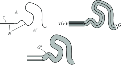
Figure 7. Gaskets $G$, $G^{\ast}$, and flange $T(r)$ for a hyperplane unknotting problem.

Since $r$ is, by hypothesis, unknotted in $N$, this $G^{\ast}$ is easily seen to be a gasket; it has three boundary components. Note that the three closed complementary components of $\text{Int}G^{\ast}$ in $\mathbb{R}^{m}$ are respectively isomorphic to $A$, $A^{\prime}$ and $T(r)$.

Since $T(r)$ is cat degree $+1$ isomorphic to $\mathbb{R}^{m}_{+}$, it is a CSI flange, and we conclude from the definition of CSI that the CSI pair $(\mathbb{R}^{m},T(r))$ is (up to CSI pair isomorphism) a CSI product $\alpha\alpha^{\prime}$, whose coarse and fine gaskets are $G$ and $G^{\ast}$.

Since $r$ is, by hypothesis, unknotted in $\mathbb{R}^{m}$, it follows, by pl and diff ambient regular neighborhood uniqueness (see Section3), that the complement of ${\textnormal{Int}}\,T(r)$ in $\mathbb{R}^{m}$ is cat isomorphic to $\mathbb{R}^{m}_{+}$. Therefore

(†) $$(\mathbb{R}^{m},T(r))\cong(\mathbb{R}^{m},\mathbb{R}^{m}_{+})=\varepsilon,$$

where $\cong$ denotes CSI pair isomorphism.

Taken together, the last two paragraphs prove the assertion that $\alpha\alpha^{\prime}\cong\varepsilon$. ∎

The assertion quickly implies the theorem using the Eilenberg-Mazur swindle. First, $\varepsilon\cong\alpha\alpha^{\prime}\cong\alpha^{\prime}\alpha$ using commutativity, so $\alpha$ and $\alpha^{\prime}$ are mutually inverse. Whence, the infinite product swindle using associativity

$$\alpha\cong\alpha\varepsilon\varepsilon\varepsilon\cdots\cong\alpha(\alpha^{\prime}\alpha)(\alpha^{\prime}\alpha)\cdots\cong(\alpha\alpha^{\prime})(\alpha\alpha^{\prime})(\alpha\alpha^{\prime})\cdots\cong\varepsilon\varepsilon\varepsilon\cdots\cong\varepsilon.$$

Also, $\alpha^{\prime}\cong\alpha^{\prime}\varepsilon\cong\alpha^{\prime}\alpha\cong\varepsilon$. Thus, $A$ and $A^{\prime}$ are cat isomorphic to $\mathbb{R}^{m}_{+}$ as required. This establishes the HLT (Theorem6.1) for $m\geq 3$ and cat=pl or cat=diff. ∎

Proof of the HLT (Theorem6.1) for $m\geq 3$ and cat$=$top.

Like Cantrell, we will use only elementary arguments. In particular, recall that, by using our refined version of the definition of CSI for top pairs given at the end of Section2, we have avoided use of the Stable Homeomorphism Theorem (=SHT) in establishing the basic properties of CSI.

We now proceed to adapt to top the above proof of the diff version. It adapts routinely except for the two short paragraphs that apply, to the ray $r$ in $\mathbb{R}^{m}$, the uniqueness of diff regular neighborhoods to deduce the diff CSI pair isomorphism († ‣ Proof of Assertion6.5). For top, we now establish († ‣ Proof of Assertion6.5) using the top open regular neighborhood uniqueness of Section3.

We can and do choose a linear structure on $N$ such that $r$ is a linear ray in $N$. The top bicollar neighborhood $G$ of $N$ was first established by M.Brown in[Bro62]; a pleasant alternative construction is due to R.Connelly, see[KS77, EssayI,p.40]. This $G$ can then be viewed as a diff gasket of which $r$ and $N$ are smooth submanifolds. However, the inclusion of $G$ into $\mathbb{R}^{m}$ is in general not a diff embedding. Let $T(r)$ be a diff regular neighborhood of $r$ in $G$ and let $G^{\ast}=G-\text{Int}T(r)$ be the resulting fine gasket.

Assertion 6.6.

The closed complement of ${\textnormal{Int}}\,T(r)$ in $\mathbb{R}^{m}$ is top isomorphic to $\mathbb{R}^{m}_{+}$. Hence, († ‣ Proof of Assertion6.5) holds for top CSI pair isomorphism.

Proof of Assertion6.6.

By hypothesis, $r$ is unknotted in $\mathbb{R}^{m}$. Thus, we can now observe that:

(1) $\mathbb{R}^{m}$ is an open topological mapping cylinder neighborhood of $r$ in $\mathbb{R}^{m}$.

(2) The diff regular neighborhood $T(r)$ in $G$ is a closed mapping cylinder neighborhood of $r$ in $\mathbb{R}^{m}$ with topological frontier ${\partial}T(r)$ bicollared in $\mathbb{R}^{m}$.

For (1), define $f:\mathbb{R}^{m-1}\to r=[0,\infty)$ by $f(x)=\left\|x\right\|$ which is a proper surjection. The mapping cylinder $\text{Map}(f)$ embeds homeomorphically onto $\mathbb{R}^{m}$ by the quotient map $F:\mathbb{R}^{m-1}\times[0,\infty)\to\mathbb{R}^{m}$ that extends $(0,x)\mapsto(0,f(x))$ and maps each hemisphere with center the origin onto the full sphere containing it, crushing (only) the hemisphere boundary onto a single point of $r$ (see Figure8).

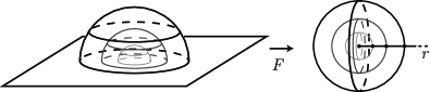
Figure 8. Quotient map $F:\mathbb{R}^{m-1}\times[0,\infty)\to\mathbb{R}^{m}$.

Fact (2) follows similarly from our peculiar definition of diff regular neighborhood of a ray (see Section3).

By open mapping cylinder uniqueness (Theorem3.4), these two facts imply that the closed complement in $\mathbb{R}^{m}$ of $\text{Int}\,T(r)$ is top isomorphic to ${\partial}T(r)\times[1,\infty)$. This completes the proof of the assertion. ∎

The proof of the HLT (Theorem6.1) for top now concludes as in the diff case. ∎

Remark 6.7.

In the above elementary proof of the top version of the HLT (Theorem6.1), it is not proved that the self homeomorphism $g$ of $\mathbb{R}^{m}$ sending $N$ to a linear hyperplane can be chosen ambient isotopic to a linear map. It is always ambient isotopic, but to prove this one needs the SHT of[Kir69, FQ90].

We close this section with some historical remarks on the Cantrell-Stallings theorem.

(1) Progress towards the top theorem from Mazur[Maz59] 1959 to Cantrell’s full top unknotting theorem in[Can63] 1963 was incremental. In 1960, Marston Morse[Mor60] extended[Maz59] to prove the top version under the extra hypothesis that $N\cup\infty$ is a top bicollared $(m-1)$-sphere in the $m$-sphere $\mathbb{R}^{m}\cup\infty$. Morton Brown’s parallel but amazingly novel article[Bro60] 1960 achieved this, too. Then Brown[Bro62] 1962 proved a collaring theorem that replaced the above bicollaring hypothesis by local flatness in the $m$-sphere $\mathbb{R}^{m}\cup\infty$. From 1962 onwards, Cantrell’s goal (reached already in 1963) has been viewed as the problem of proving that a codimension $1$ sphere in a sphere of dimension $>3$ cannot have a single ‘singular’ point where local flatness fails.

(2) Huebsch and Morse[HM62] 1962 established the diff version under the much stronger unknotting hypothesis that $N$ be linear outside a bounded set in $\mathbb{R}^{m}$.

(3) Our proof (for any cat) can be viewed as a radical reorganization using CSI of Cantrell’s proof for top[Can63]. On the other hand, it was Stallings[Sta65] who first pointed out the diff version, and formulated a version valid in all dimensions. The proof of the top version requires extra precautions (for us, diff gaskets) and extra argumentation (for us, open mapping cylinder neighborhood uniqueness), but, in compensation, it clearly reproves, ab initio, the Schoenflies theorem of Mazur[Maz59] and Brown[Bro60, Bro62].

(4) The apparent novelty, which made us write down the above proof, was our reformulation (circa 2002) of much of the geometry of Cantrell’s proof as standard facts about CSI. This explicit use of some sort of connected sum was, of course, suggested by Mazur’s pioneering article[Maz59]; compare the ‘almost pl’ version of the Schoenflies theorem in[RS72].

(5) CSI itself was not a novelty. Gompf[Gom85] had showed that an infinite CSI of smooth $4$-manifolds, each homeomorphic to $\mathbb{R}^{4}$, is well defined. He achieved this by proving a multiple ray unknotting result using finger moves; his proof readily extends to all dimensions $\geq 4$ (in fact, it is simpler in dimensions $>4$). Gompf used this observation and the infinite product swindle to show that an exotic $\mathbb{R}^{4}$ cannot have an inverse under CSI. The reader can now check this as an exercise.

(6) Stallings[Sta65] deals explicitly only with the diff case. He avoids all connected sum notions. Indeed, the basic entity for which he defines an infinite product operation is a (proper) diff embedding $f:\mathbb{R}^{m-1}\to\mathbb{R}^{m}$ (with an unknotted ray and $m\geq 3$). Stallings’ exposition seems to invite formalization in terms of a pairwise CSI operation.

(7) Johannes de Groot 1972[deG72] announced a proof of Cantrell’s top HLT by generalization of M.Brown’s proof of the top Schoenflies theorem. Regrettably, de Groot died shortly thereafter and no manuscript has surfaced since.

7. Basic Ray Unknotting in Dimensions ¿ 3

The first goal of this section is to explain the well known fact, mentioned in Remark6.2 above, that rays in $\mathbb{R}^{m}$ are related by an ambient isotopy provided that $m>3$. Then we go on, still assuming $m>3$, to classify so called multirays in terms of the proper homotopy classes of their component rays.

Throughout this section, cat is one of top, pl or diff. The following basic result will be needed for $1$-manifolds mapping into manifolds of dimension $m>3$.

Theorem 7.1 (Stable Range Embedding Theorem).

Let $f:N^{n}\to M^{m}$ be a proper continuous map of cat manifolds, possibly with boundary. If $2n+1\leq m$, then $f$ is properly homotopic to a cat embedding $g:N\to M$ such that $g(N)$ lies in ${\textnormal{Int}}M$. Further, if $2n+2\leq m$ and $g^{\prime}$ is a second such embedding properly homotopic to $f$, then there exists a cat ambient isotopy $h_{t}:M\to M$, $0\leq t\leq 1$, such that $h_{0}=\textnormal{id}|_{M}$ and $h_{1}g=g^{\prime}$.

For cat=pl or cat=diff, the proof is a basic general position argument that can be found in many textbooks. Early references are[Whi36] and[BK64].

For top, the proof is still surprisingly difficult. One needs a famous method of T.Homma from 1962[Hom62], as applied by H.Gluck[Glu63, Glu65]. Many expositions of these types of results (in particular[Glu65]) are given in a compact relative form, from which one has to deduce the stated noncompact, nonrelative but proper version by a classic argument involving a skeletal induction in the nerve of a suitable covering (see Essay I, Appendix C in[KS77]).

Next, we show that, in some cases of current interest, all rays are properly homotopic.

Lemma 7.2 (Simplest Proper Ray Homotopies).

Let $X$ be locally arcwise connected and locally compact. Suppose $X$ admits a connected closed collar neighborhood $Y\times[0,\infty)$ of Alexandroff infinity. Then any two proper maps $[0,\infty)\to X$ are properly homotopic.

Proof.

Any proper map $f:[0,\infty)\to X$ is proper homotopic to one with image in the closed subset $Y\times[0,\infty)\subset X$, so we can and do assume that $X$ is $Y\times[0,\infty)$.

Then, writing $f(0)=(y,t_{0})\in Y\times[0,\infty)$, it is easy to construct an explicit proper homotopy of $f$ to the proper continuous radial embedding $r_{y}:[0,\infty)\hookrightarrow X=Y\times[0,\infty)$ sending $t\mapsto(y,t)$ for all $t$.

Finally, for any two points $y$ and $y^{\prime}$ in $Y$, there is a path from $y$ to $y^{\prime}$ in $Y$ and any such path provides an explicit proper homotopy from $r_{y}$ to the similarly defined radial embedding $r_{y^{\prime}}$. ∎

These last two results, when combined with the Cantrell-Stallings theorem as stated in the last section (Theorem6.1), yield the following Hyperplane Linearization Theorem already announced there.

Theorem 7.3.

For $m\neq 3$, any cat submanifold $N$ of $\mathbb{R}^{m}$ that is isomorphic to $\mathbb{R}^{m-1}$ is unknotted in the sense that there is a cat automorphism $h$ of $\mathbb{R}^{m}$ such that $h(N)=\mathbb{R}^{m-1}\times 0\subset\mathbb{R}^{m}$.

Remarks 7.4.

(1) Remember that, by convention, a cat submanifold is a closed subset and is assumed cat locally flat unless the contrary is explicitly stated.

(2) The case cat=top of Theorem7.3 is Cantrell’s result as he formulated it. Beware that (still today) any completely bootstrapping proof seems to require an exposition of Homma’s method.

(3) It is well known that a proper ray (any cat) may be knotted in $\mathbb{R}^{3}$. Fox and Artin[FA48, Example1.2] exhibited the first such ray, Alford and Ball[AB63] produced infinitely many knot types and conjectured uncountably many exist, and McPherson[McP73] published a proof of this conjecture (earlier, Giffen 1963, Sikkema, Kinoshita, and Lomonaco 1967, and McPherson 1969 had announced proofs[BC71, p.273]). The boundary of a closed regular neighborhood of any such knotted ray is a knotted hyperplane in $\mathbb{R}^{3}$. Still, even in this dimension the knot type of any cat hyperplane $N\subset\mathbb{R}^{3}$ is determined by the knot type in $\mathbb{R}^{3}$ of any cat ray $r\subset N$[Sik66] (see also[HM53]); in fact, $N$ is ambient isotopic to the boundary of a cat closed regular neighborhood of $r$ in $\mathbb{R}^{3}$[CK10]. Thus, one of the two closed complementary components of $N$ in $\mathbb{R}^{3}$ is cat isomorphic to $\mathbb{R}_{+}^{3}$.

(4) Here is an immediate corollary for cat = diff that concerns the still mysterious dimension 4. Suppose that $N^{3}\subset S^{4}$ is a smoothly embedded $3$-sphere such that the pair $(S^{4},N^{3})$ is not diff isomorphic to $(S^{4},S^{3})$ and thus is a counterexample to the unsettled diff $4$-dimensional Schoenflies conjecture. Then, nevertheless, for any point $p$ in $N^{3}$ one has $(S^{4}-p,N^{3}-p)\cong(\mathbb{R}^{4},\mathbb{R}^{3})$.

(5) We have seen that the Cantrell-Stallings unknotting theorem is closely related to the fact that: if $\alpha:=(M,P)$ is a dimension $m$ cat CSI pair that has an inverse up to degree $+1$ isomorphism in the commutative semigroup of isomorphism classes of cat CSI pairs of dimension $m\geq 3$ under CSI sum, then $(M,P)$ is in the identity class, namely that of $(\mathbb{R}^{m},\mathbb{R}_{+}^{m})$. Thus it is perhaps of interest to ask about other algebraically expressible facts about this semigroup. For example: is it true that $\alpha\cong\alpha\beta$ always implies that $\alpha\cong\alpha\beta^{\infty}$? Curiously, this is false for certain $(M,P)$ where $M$ has more than one end, as Figure9 indicates.

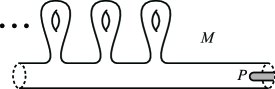
Figure 9. CSI pair $(M,P)$ where $M$ has two ends and one end is collared.

Although this figure is for dimension $2$, it clearly has analogs in all dimensions $>2$. Is this implication true at least when $M$ has one end? Or when $M$ is the interior of a compact manifold?

This concludes our exposition of the Cantrell-Stallings theorem.

8. Singular and Multiple rays

This section shows that multiple rays embed and unknot much like single rays. We define a singular ray in a locally compact space $X$ to be a proper continuous map $[0,\infty)\to X$. In Section9, singular rays will be a tool for unknotting multiple hyperplanes in dimensions $>3$.

Lemma 8.1.

Let $f_{i}:[0,\infty)\to X$, with $i$ varying in the finite or countably infinite discrete index set $S$, be singular rays in a locally compact, sigma compact space $X$. Then, for each $i\in S$, one can choose a proper homotopy of $f_{i}$ to a singular ray $f^{\prime}_{i}$ such that the rule $(i,x)\mapsto f^{\prime}_{i}(x)$ defines a proper map $f^{\prime}:S\times[0,\infty)\to X$.

Proof.

The choice $f_{i}=f^{\prime}_{i}$ will do, in case $S$ is finite. When $S$ is infinite, we can assume $S=\mathbb{Z}_{+}$. Then, choose in $X$ a sequence of compacta $\emptyset=K_{1}\Subset K_{2}\Subset K_{3}\Subset\cdots$ with $X=\cup_{j}K_{j}$. By properness of $f_{i}$, there exists $a_{i}$ in $[0,\infty)$ so large that $f_{i}([a_{i},\infty))\subset X-K_{i}$. Define $f^{\prime}_{i}$ to be $f_{i}$ precomposed with the retraction $[0,\infty)\to[a_{i},\infty)$.

It is easily seen that $f^{\prime}_{i}$ is properly homotopic to $f_{i}$. The properness of the resulting $f^{\prime}_{i}$ now follows. Indeed, if $K\subset X$ is compact, then $K$ lies in the interior of $K_{i}$ for some $i$, hence $f^{\prime}_{j}([0,\infty))\cap K=\emptyset$ for $j>i$. Thus, the preimage $f^{\prime-1}(K)$ in $S\times[0,\infty)$ meets $j\times[0,\infty)$ only for $j\leq i$. But, the intersection $f^{\prime-1}(K)\cap\{1,2,\dots,i\}\times[0,\infty)$ is compact by the finite case. ∎

Here is a key lemma concerning just one singular ray that will help to deal with infinitely many rays.

Lemma 8.2.

Let $K$ be a given compact subset of a locally compact, sigma compact space $X$ and let $f$ and $f^{\prime}$ be singular rays in $X$ whose images are disjoint from $K$. If $f$ and $f^{\prime}$ are properly homotopic in $X$, then the proper homotopy can be (re)chosen to have image disjoint from $K$.

Proof.

If $h_{t}:[0,\infty)\to X$, $0\leq t\leq 1$, is a proper homotopy from $f=h_{0}$ to $f^{\prime}=h_{1}$, then its properness assures that for some $d\geq 0$ the image $h_{t}([d,\infty))$ is disjoint from $K$ for all $t$. But, the singular ray $f$ is proper homotopic in the complement of $K$ to the singular ray $\widehat{f}$ that is $f|_{[0,\infty)}$ precomposed with the retraction $[0,\infty)\to[d,\infty)$. Similarly for $f^{\prime}$. Shunting together these three proper homotopies, one obtains the asserted proper homotopy. ∎

Lemma 8.3.

Let $f_{i}$ and $f^{\prime}_{i}$, with $i$ varying in the finite or countably infinite discrete set $S$, be two indexed sets of singular rays in the connected, locally compact, sigma compact space $X$. Suppose that the two continuous maps $f$ and $f^{\prime}$ from $S\times[0,\infty)$ to $X$ defined by the rules $(i,x)\mapsto f_{i}(x)$ and $(i,x)\mapsto f_{i}^{\prime}(x)$ are both proper. Suppose also that $f_{i}$ is proper homotopic to $f^{\prime}_{i}$ for all $i\in S$. Then, there exists a proper homotopy $h_{t}:S\times[0,\infty)\to X$, $0\leq t\leq 1$, that deforms $h_{0}=f$ to $h_{1}=f^{\prime}$.

Proof.

We propose to define the wanted proper homotopy $h_{t}$ by choosing, for $i\in S$, suitable proper homotopies $h_{i,t}$ from $f_{i}$ to $f^{\prime}_{i}$ and then defining $h_{t}$ by setting $h_{t}(i,x)=h_{i,t}(x)$ for all $i\in S$, all $t\in[0,1]$, and all $x\in[0,\infty)$. The choices aim to assure that $h_{t}$ is a proper homotopy – which means that the rule $(t,i,x)\mapsto h_{t}(i,x)$ is proper as a map $[0,1]\times S\times[0,\infty)\to X$.

If $S$ is finite, any choices will do. But, if $S$ is infinite, then bad choices abound. For example, $h_{t}$ is not proper if every homotopy $h_{i,t}(x)$ meets a certain compactum $K$.

If $S$ is infinite, we now specify choices that do the trick. Without loss, assume $S=\mathbb{Z}_{+}$. Let $\emptyset=K_{1}\Subset K_{2}\Subset K_{3}\Subset\cdots$ be an infinite sequence of compacta with $X=\cup_{j}K_{j}$. For each $i\in S$, let $J(i)$ be the greatest positive integer such that the images of the singular rays $f_{i}$ and $f^{\prime}_{i}$ are both disjoint from $K_{J(i)}$. Since $f$ and $f^{\prime}$ are proper, $J(i)$ tends to infinity as $i$ tends to infinity. Use Lemma 8.2 to choose the proper homotopy $h_{i,t}$ from $f_{i}$ to $f^{\prime}_{i}$ to have image disjoint from $K_{J(i)}$. Then, the properness of the resulting $h_{t}$ is verified as in the proof of Lemma 8.1. ∎

Remark 8.4.

Lemmas8.1 to8.3 above hold good with $[0,\infty)$ replaced by its product with (varying) compacta.

Define a multiray in the cat manifold $M^{m}$ to be a cat submanifold lying in $\text{Int}M$ each component of which is a ray. Combining the Stable Range Embedding Theorem (Theorem7.1) with Lemmas8.1 to8.3 concerning proper maps, we get

Proposition 8.5 (Classifying Multirays via Proper Homotopy).

Let $M^{m}$ be a connected noncompact cat manifold, and let $f_{i}$ be singular rays where $i$ ranges over a finite or countably infinite index set $S$. If $m\geq 3$, then $f_{i}$ is properly homotopic to a cat embedding $g_{i}$ onto a ray, such that the rules $(i,x)\mapsto g_{i}(x)$ collectively define a (proper) cat embedding $g:S\times[0,\infty)\to M$ with image a multiray. Furthermore, if $m>3$ and $g^{\prime}_{i}$ is an alternative choice of the ray embeddings $g_{i}$, resulting in the alternative cat embedding $g^{\prime}$ onto a multiray, then there exists an ambient isotopy $h_{t}:M\to M$, $0\leq t\leq 1$, such that $h_{0}=\textnormal{id}|_{M}$ and $h_{1}g=g^{\prime}$. ∎

9. Multiple Component Hyperplane Embeddings

In this section we investigate proper cat embeddings into $\mathbb{R}^{m}$ of a disjoint sum of at most countably many disjoint hyperplanes, each isomorphic to $\mathbb{R}^{m-1}$.

For cat=top we will, for the first time, make essential use of the Stable Homeomorphism Theorem (=SHT) to show that every self homeomorphism of $\mathbb{R}^{k}$ is ambient isotopic to a linear one[Kir69, FQ90]; this is equivalent to $\pi_{0}(\text{STop}(k))=0$, where STop$(k)$ is the group of orientation preserving self homeomorphisms of $\mathbb{R}^{k}$ endowed with the compact open topology. Not to do so would lead to pointless hairsplitting.

In these circumstances, we can and do revert to the unrefined versions of the definition for top of the CSI operation and its related constructions. We use the following lemma.

Lemma 9.1.

If $G$ and $G^{\prime}$ are top gaskets and $f:{\partial}G\to{\partial}G^{\prime}$ is a degree $+1$ top isomorphism of their boundaries, then $f$ extends to a degree $+1$ top isomorphism $F:G\to G^{\prime}$.

Proof.

By definition of gasket (see Section2), we may assume $G$ and $G^{\prime}$ are linear gaskets. By the SHT, we can isotop $f$ to a diff isomorphism $f^{\prime}$. This $f^{\prime}$ extends to a degree $+1$ diff isomorphism $F^{\prime}:G\to G^{\prime}$ by the diff version of this lemma (Corollary4.5 above). Using closed collars of ${\partial}G$ and ${\partial}G^{\prime}$ we easily construct the asserted top isomorphism $G\to G^{\prime}$. ∎

A multiple hyperplane is a properly embedded submanifold $N$ of $\mathbb{R}^{m}$ where $N$ is the disjoint union of components $N_{i}\cong\mathbb{R}^{m-1}$ for $i\in S$, and $S$ is a nonempty countable index set. We say that $G$, the closure of a component of $\mathbb{R}^{m}-N$ in $\mathbb{R}^{m}$, is docile if it is a gasket, and we say that $N$ itself is docile if the closure of every such component is docile.

Given any multiple hyperplane $N$ in $\mathbb{R}^{m}$, we can construct a canonical simplicial tree $T$ as follows. The vertices $V$ of $T$ are the closures of the complementary components of $N$ in $\mathbb{R}^{m}$. An edge is a component $N_{i}$ of $N$ and it joins the two vertices $u,v\in V$ whose intersection is $N_{i}$. The tree $T$ is clearly well defined by the pair $(\mathbb{R}^{m},N)$ up to tree isomorphism; it is the nerve of the covering of $\mathbb{R}^{m}$ by the closures of the components of $\mathbb{R}^{m}-N$. Also, $T$ is at most countable, but it is not necessarily locally finite. If $m=2$, then these trees are naturally planar as the edges at each vertex are cyclically ordered.

Conversely, given such a tree $T$ (planar in case $m=2$), there is a natural recipe to construct a multiple hyperplane $N$ in $\mathbb{R}^{m}$ where the closure of each complementary component is a gasket as follows. For each vertex $v_{k}\in V$, pick a gasket $G_{k}$ with boundaries corresponding bijectively to the edges incident with $v_{k}$ in $T$. Gluing these gaskets together according to $T$ gives a composite gasket $TG$ with empty boundary.

It was established in proving the associativity property of CSI that there is a cat manifold isomorphism $TG\to\mathbb{H}^{m}$ sending each vertex gasket in $TG$ to a linear gasket in $\mathbb{H}^{m}$ and, hence, each edge hyperplane to a hyperbolic hyperplane in $\mathbb{H}^{m}$ (see Lemma5.2 above). Further, such an isomorphism is unique up to degree $+1$ cat isomorphism of $\mathbb{H}^{m}$.

We now summarize these observations, where cat is top, pl or diff.

Theorem 9.2 (Multiple Hyperplane Linearization Thm. (=MHLT)).

For $m$ distinct from $3$, every cat multiple hyperplane embedding $N$ in $\mathbb{R}^{m}$ is docile. Hence, for $m>3$, such embeddings are naturally classified modulo ambient degree $+1$ cat automorphism by arbitrary countable simplicial trees modulo simplicial tree automorphisms. For $m=2$ (and only $m=2$) one must use planar trees and their planar tree automorphisms (where planar here means that, at each vertex, the edges are cyclicly ordered).

Corollary 9.3 (Gasket Recognition Theorem (=GRT)).

Consider a cat $m$-manifold with nonempty boundary whose interior is isomorphic to ${\mathbb{R}}^{m}$, and for which every boundary component is isomorphic to ${\mathbb{R}}^{m-1}$. Exclude the case $m=3$. Then $M$ is isomorphic to a linear gasket. ∎

Proof of the GRT (Corollary9.3).

${\textnormal{Int}}\,M$ is always isomorphic to the manifold obtained by adding to $M$ an external open collar along $\partial{M}$. ∎

Corollary 9.4.

With the same data as in the MHLT and assuming $m\geq 4$, the pair $(\mathbb{R}^{m},N)$ is cat isomorphic to a Cartesian product

$$(\mathbb{H}^{2},N^{\prime})\times\mathbb{R}^{m-2}$$

where each component of $N^{\prime}$ is a hyperbolic line. ∎

Proof of the MHLT (Theorem9.2) for $m>3$ and cat$=$pl or diff.

Let $G$ be the closure of a component of $\mathbb{R}^{m}-N$ in $\mathbb{R}^{m}$. Reindex so that $N_{i}$, $i\in S$, are the boundary components of $G$. For each $N_{i}$, let $V_{i}$ denote the closed component of $\mathbb{R}^{m}-\text{Int}G$ with boundary $N_{i}$. Each $N_{i}$ is unknotted in $\mathbb{R}^{m}$ by the cat HLT (Theorem7.3). Therefore, for each $i\in S$ there is a cat proper ray $r_{i}\subset\text{Int}V_{i}$ so that $V_{i}$ is a cat regular neighborhood of $r_{i}$ in $\mathbb{R}^{m}$. As $N\subset\mathbb{R}^{m}$ is a proper submanifold, the union of the rays $r_{i}$ is a proper multiray in $\mathbb{R}^{m}$.

Choose $G^{\prime}\subset\mathbb{H}^{m}$ a linear gasket with boundary hyperplanes $N^{\prime}_{i}$, $i\in S$. For each $N^{\prime}_{i}$, let $V^{\prime}_{i}$ denote the closed component of $\mathbb{H}^{m}-\text{Int}G^{\prime}$ with boundary $N^{\prime}_{i}$ and let $r^{\prime}_{i}\subset\text{Int}V^{\prime}_{i}$ be a radial ray. Plainly, $V^{\prime}_{i}$ is a cat regular neighborhood of $r^{\prime}_{i}$ for each $i\in S$ and the union of the rays $r^{\prime}_{i}$ is a proper multiray in $\mathbb{H}^{m}$.

Choose a cat isomorphism $\psi:\mathbb{R}^{m}\rightarrow\mathbb{H}^{m}$. cat proper multirays unknot in $\mathbb{H}^{m}$, $m>3$, by the basic cat Stable Range Embedding Theorem (Theorem7.1), proved by general position, and Lemmas7.2 and8.3. Thus, there is an ambient isotopy of $\mathbb{H}^{m}$ carrying $\psi(r_{i})$ to $r^{\prime}_{i}$ for all $i\in S$ simultaneously. So, we may as well assume $\psi(r_{i})=r^{\prime}_{i}$ for $i\in S$. By pl and diff regular neighborhood ambient uniqueness (see Section3), we may further assume that $\psi(V_{i})=V^{\prime}_{i}$ for all $i\in S$. Then, $\psi|_{G}:G\rightarrow G^{\prime}$ is a cat isomorphism as desired. ∎

Proof of the MHLT (Theorem9.2) for $m>3$ and cat$=$top.

Again, let $G$ be the closure of a component of $\mathbb{R}^{m}-N$ in $\mathbb{R}^{m}$ and reindex so that $N_{i}$, $i\in S$, are the boundary components of $G$. We have three cases depending on the number $\left|S\right|$ of boundary components of $G$.

Case $\left|S\right|=1$.

This is exactly Cantrell’s top HLT (Theorem7.3). ∎

Case $\left|S\right|=2$.

This case is well known as the Slab Theorem and is a worthy sequel by C.Greathouse[Gre64b] 1964 to Cantrell’s top HLT (Theorem7.3), so we include a proof. Greathouse deduced it from results then recently established, together with the following (for $m>3$) then unproved.

Theorem 9.5 (Annulus Conjecture (=AC$(m)$)).

If $S_{1}$ and $S_{2}$ are two disjoint locally flatly embedded $(m-1)$-spheres in $S^{m}$ and $X$ is the closure of the component of $S^{m}-(S_{1}\cup S_{2})$ with $\partial{X}=S_{1}\sqcup S_{2}$, then $X$ is homeomorphic to the standard annulus $S^{m-1}\times[0,1]$.

This Annulus Conjecture was later proved, along with the SHT, in [Kir69] 1969 for $m>4$, and in[FQ90] 1990 for $m=4$ (see also[Edw84]). The already proved results used in[Gre64b] included Cantrell’s top HLT, that we have reproved (Theorem7.3), and the following, proved by Cantrell and Edwards[CE63] 1963.

Lemma 9.6 (Arc Flattening Lemma).

If a compact arc $A$ topologically embedded in $S^{m}$, $m>3$, is locally flat except possibly at one interior point $P$, then $A$ is locally flat also at $P$.

Assuming these tools for the moment, we now give:

Proof of the Slab Theorem.

We consider the sphere $S^{m}$ to be $\mathbb{R}^{m}\cup\infty$. Let $G_{i}$, $i=1,2$, be the components of $\mathbb{R}^{m}-{\textnormal{Int}}G$. By the top HLT (Theorem7.3), each $G_{i}\cong\mathbb{R}_{+}^{m}$. Hats will indicate the adjunction of the point $\infty\in S^{m}$. Enlarge $\widehat{G}:=G\cup\infty$ by adding to it a closed collar $C_{i}$ of the $(m-1)$-sphere $\partial{\widehat{G}_{i}}$ in $\widehat{G}_{i}$, for $i=1,2$. Denote the result $X:=\widehat{G}\cup C_{1}\cup C_{2}$. This is a top submanifold of $S^{m}$ with boundary two $(m-1)$-spheres $S_{1}$ and $S_{2}$, where $S_{i}$, for $i=1$ and $2$, is the component of $\partial{C_{i}}$ disjoint from $\widehat{G}$ (see Figure10).

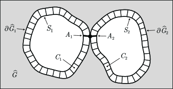
Figure 10. Almost global view of $\widehat{G}$ in $S^{m}=\mathbb{R}^{m}\cup\infty$, focused on the point $\infty=A_{1}\cap A_{2}$.

The theorem AC$(m)$ (Theorem9.5) tells us that $X\cong S^{m-1}\times[0,1]$. Furthermore, we have collaring identifications $C_{i}=S_{i}\times[0,1]$. Consider the locally flat arc $A_{i}$ that is the arc fiber of the collaring $C_{i}=S_{i}\times[0,1]$ that contains $\infty\in S^{m}$. Clearly $A_{1}\cap A_{2}=\infty$; thus $A:=A_{1}\cup A_{2}$ is an arc in $X$ that is locally flat except possibly at $\infty\in S^{m}$. By the above Arc Flattening Lemma (Lemma9.6), $A$ is locally flat at $\infty$; hence it is a locally flat $1$-submanifold of $X$ joining the two boundary components of $X$. Note that $G\cong X-A$ by Brown’s collaring uniqueness theorem[Bro62].

By the uniqueness clause of the elementary (but subtle!) top version of the Stable Range Embedding Theorem (Theorem7.1), any two such arcs are related by a top automorphism of $X\cong S^{m-1}\times[0,1]$. Thus the complement $X-A$ is homeomorphic to $\mathbb{R}^{m-1}\times[0,1]$. ∎

Proof of the Arc Flattening Lemma.

Split $A$ at $P$ to get two compact arcs $A_{1}$ and $A_{2}$ with $A_{1}\cap A_{2}=P$.

Assertion 9.7.

There exists a compact locally flat $n$-ball neighborhood $B$ of ${\textnormal{Int}}\,A_{1}$ such that $A_{1}$ is unknotted in $B$ and $B$ is disjoint from ${\textnormal{Int}}\,A_{2}$.

Proof of Assertion9.7.

In our one application of the Arc Flattening Lemma above (namely to prove the Slab Theorem), $B$ can obviously be any tubular neighborhood of $A_{1}$ in $C_{1}$ derived from the product structure $C_{1}=S_{i}\times[0,1]$. Thus we leave the full proof of this assertion to the interested reader with just this hint: $B$ can in general be the closure in $S^{m}$ of a suitably tapered trivial normal tubular neighborhood of ${\textnormal{Int}}A_{1}$ in $S^{m}$ (see[Lac67]). ∎

Now, by the top Schoenflies theorem, $S^{m}-{\textnormal{Int}}B$ is also an $m$-ball $B^{\prime}$ in $S^{m}$. In $B^{\prime}$ the second arc $A_{2}$ is embedded in a manner that is locally flat except possibly at $P\in\partial{B^{\prime}}$. To the non-compact top manifold $B^{\prime}-P\cong\mathbb{R}_{+}^{m}$ we apply the uniqueness clause of the Stable Range Embedding Theorem (Theorem7.1); we conclude, on recompactifying in $S^{m}$, that the arc $A_{2}$ is unknotted in $B^{\prime}$. It follows that the arc $A:=A_{1}\cup A_{2}$ is locally flat in $S^{m}$. This completes our proof of the Arc Flattening Lemma (Lemma9.6). ∎

Assuming AC$(m)$ (now known!), this completes the proof of the Slab Theorem which is the MHLT (Theorem9.2) for the case when $G$ has two boundary components. ∎

Remarks 9.8.

(1) Greathouse[Gre64a] 1964 also proved that the Slab Theorem in dimension $m$ implies AC$(m)$, granting results known in 1964 that we have mentioned. Hints: given an $m$-annulus $X$ in $S^{m}$, form a locally flat arc $A\subset X$ joining the two boundary $(m-1)$-spheres. Show that $A$ is cellular (i.e., an intersection of compact $m$-cell neighborhoods in $S^{m}$) so that the quotient space $(S^{m}/A)$ is homeomorphic to $S^{m}$, and apply the Slab Theorem to show that $X-A\cong\mathbb{R}^{m-1}\times[0,1]$. Deduce that $X\cong S^{m-1}\times[0,1]$ with the help of collarings and the Mazur-Brown Schoenflies theorem.

(2) An easy argument shows that AC$(n)$ (Theorem9.5), $n=1,\ldots,m$, together imply the following.

Theorem 9.9 (Stable Homeomorphism Conjecture (=SHC$(m)$)).

For any homeomorphism $h:\mathbb{R}^{m}\to\mathbb{R}^{m}$, there exists a homeomorphism $h^{\prime}:\mathbb{R}^{m}\to\mathbb{R}^{m}$ that coincides with $h$ near the origin and with the identity map outside a bounded set.

Hint: For this implication, you will need some Alexander isotopies. Exactly this form of the SHC$(m)$ was proved for $m\geq 5$ by R.Kirby in[Kir69].

(3) An easy argument establishes the implication SHC$(m)$ $\Rightarrow$ AC$(m)$.

Proof of the MHLT (Theorem9.2) for cat$=$top and $\left|S\right|>2$.

Let $G$ be the closure in $\mathbb{R}^{m}$ of a component of $\mathbb{R}^{m}-N$. Let $N_{i}$, $i\in S$, be an indexing of the components of $\partial{G}$. For each $N_{i}$, let $V_{i}$ denote the closed component of $\mathbb{R}^{m}-\text{Int}G$ with boundary $N_{i}$. By the top HLT (Theorem7.3), each $V_{i}$ is top isomorphic to closed upper half space $\mathbb{R}^{m}_{+}$. It is straightforward to produce, for each $i\in S$, a diff proper ray $r_{i}\subset\text{Int}V_{i}$. Let $T(r_{i})\subset\text{Int}V_{i}$ be a diff (closed) regular neighborhood of $r_{i}$. The boundary $H_{i}$ of $T(r_{i})$ is a diff hyperplane. By the Slab Theorem, the closure of the region between $H_{i}$ and $N_{i}$ is top isomorphic to $\mathbb{R}^{m-1}\times[0,1]$. This isomorphism yields an obvious isotopy of $N_{i}$ to $H_{i}$ for each $i\in S$. Using disjoint collars of the $H_{i}$ and $N_{i}$, these isotopies readily extend to an ambient isotopy of $\mathbb{R}^{m}$ which carries the collection $N_{i}$, $i\in S$, to the diff collection $H_{i}$, $i\in S$. The result now follows from the diff proof of the MHLT (Theorem9.2) above. ∎

This completes the proof of the MHLT (Theorem9.2) for $m>3$ and cat=top. ∎

Proof of the MHLT (Theorem9.2) for $m=2$.

We begin with the following.

Observation 9.10.

By triangulation and smoothing theorems for dimension $2$ that we refer collectively as the $2$-Hauptvermutung (see [Moi77] or[Sie05]), it suffices to establish the MHLT (Theorem9.2) for any one of the three categories cat = diff, pl, or top.

We work in the smooth category. The diff proof of the MHLT (Theorem9.2) already given for $m>3$ adapts easily to $m=2$ using the following.

Theorem 9.11 (Multiray Radialization Theorem in $\mathbb{R}^{2}$ (=$2$-MRT)).

Let $L\subset\mathbb{R}^{2}$ be a smooth proper multiray. Then $L$ is ambient isotopic to a radial multiray.

Proof of the $2$-MRT (Theorem9.11).

Translate so that $L$ misses the origin. Morse theory tells us that, by a small smooth perturbation of $L$ in $\mathbb{R}^{2}$, we may assume that

restricts to a Morse function on $L$ with distinct critical values, cf.[Mil65].

Seen in a nutshell, our proof plan is to alter $L$ by ambient isotopy to eliminate critical points of $f|_{L}$ in pairs until $f|_{L}$ has no critical points at all. Then a further ambient isotopy will make $L$ radial; this latter isotopy will arise by integration of a vector field on $\mathbb{R}^{2}$ that is tangent to $L$ (as modified so far) and is transverse to the level spheres of $f$.

Assertion 9.12.

By an ambient isotopy, we may assume that on each component $r$ of $L$ an absolute minimum of the restriction $f|_{r}$ is attained at the point $\partial{r}$ only, and this point is noncritical for $f|_{r}$.

Proof of Assertion9.12.

For each component $r_{i}$ of $L$ for which $f(\partial{r_{i}})$ is not the unique minimum point $m_{i}$ of $f$ on $r_{i}$, consider a small smooth regular neighborhood $N_{i}$ of the interval $K_{i}$ in $r_{i}$ that joins $m_{i}$ to $\partial{r_{i}}$. These $N_{i}$ can be chosen so small that their union $N$ is a disjoint sum of these $N_{i}$. Then independent smooth isotopies, each with support in one $N_{i}$, together establish the assertion (cf.[Mil97, pp.22–24]). ∎

Now, perform a possibly infinite number of steps. For convenience, we consider the points in $\partial{L}$ to be critical points of $f|_{L}$ from here on.

Step$\mathbf{1}$.

Let $u_{\mathrm{max}}$ be the local maximum of $f|_{L}$ on which $f$ assumes the minimum value. Let $r_{i}$ be the component of $L$ containing $u_{\mathrm{max}}$. Let $u_{0}$ and $u_{1}$ be the critical points of $f|_{L}$ adjacent to $u_{\mathrm{max}}$ in $r_{i}$; the only critical points in the segment from $u_{0}$ to $u_{1}$ in $r_{i}$ are $u_{0}$, $u_{\mathrm{max}}$, and $u_{1}$. After switching $u_{0}$ and $u_{1}$ if needed, we may assume $f(u_{1})>f(u_{0})$. There is a unique $u_{2}$ on the segment of $r_{i}$ from $u_{0}$ to $u_{\mathrm{max}}$ so that $f(u_{2})=f(u_{1})$.

We will ambiently cancel the index $0$ and index $1$ critical points $u_{1}$ and $u_{\mathrm{max}}$. Let $A$ denote the complement in $\mathbb{R}^{2}$ of the open disk of radius $f(u_{1})$ centered at the origin. Let $D$ be the compact region in $A$ bounded by the segment of $r_{i}$ from $u_{1}$ to $u_{2}$ and an arc of the circle of radius $f(u_{1})$ between $u_{1}$ and $u_{2}$ (see Figure11).

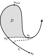
Figure 11. Cancelling pair of critical points $u_{1}$ and $u_{\mathrm{max}}$. The dotted arc indicates an arc of the circle of radius $f(u_{1})$ between $u_{1}$ and $u_{2}$. The dashed line indicates the trajectory of $h_{1}(r_{i})$ after cancellation.

Assertion 9.13.

For any neighborhood $U$ of $D$ there is a diffeomorphism $h_{1}$ of $\mathbb{R}^{2}$ so that:

(a) $f(h_{1}(x))\leq f(x)$ for all $x\in\mathbb{R}^{2}$.

(b) The support of $h_{1}$ lies in $U$.

(c) The support of $h_{1}$ does not intersect $L-r_{i}$ and also only intersects $r_{i}$ in a small neighborhood of the segment of $r_{i}$ from $u_{1}$ to $u_{2}$.

(d) The critical points of the restriction of $f$ to $h_{1}(L)$ are the same as those of $f|_{L}$, except for $u_{\mathrm{max}}$ and $u_{1}$ which are no longer critical or even in $h_{1}(L)$.

Proof of Assertion9.13.

Note that the interior of $D$ does not intersect $L$, since that would give a local maximum of $f|_{L}$ with value $<f(u_{\mathrm{max}})$, contrary to our choice of $u_{\mathrm{max}}$. Consequently, we may assume $U$ does not intersect $L-r_{i}$ and does not intersect $r_{i}$ outside a small neighborhood of the segment of $r_{i}$ from $u_{1}$ to $u_{2}$.

We get $h_{1}$ by integrating a suitable vector field $v$ on $\mathbb{R}^{2}$. All we need to do is make sure that:

$\bullet$ $v(x)\cdot x\leq 0$ for all $x\in\mathbb{R}^{2}$ (to get (a)).

$\bullet$ $v(x)\cdot x=-|x|$ for all $x$ in some neighborhood $U^{\prime}$ of $D$.

$\bullet$ $v$ points into $D$ on the interior of the segment of $r_{i}$ from $u_{1}$ to $u_{2}$.

$\bullet$ $v$ points out of $D$ on the arc of the circle of radius $f(u_{1})$ from $u_{1}$ to $u_{2}$.

$\bullet$ The support of $v$ is contained in $U$, does not intersect $L-r_{i}$, and does not intersect $r_{i}$ outside of a small neighborhood of the segment of $r_{i}$ from $u_{1}$ to $u_{2}$.

It suffices to find such a $v$ locally, since then $v$ is obtained by piecing together with a partition of unity. Finding $v$ locally is easy. The vector field $v(x)=-x/|x|$ works on the interior of $D$, on the circle of radius $f(u_{1})$ (except possibly at $u_{2}$), and near $u_{\mathrm{max}}$. On the segment of $r_{i}$ from $u_{1}$ to $u_{2}$ (but not at $u_{\mathrm{max}}$ or $u_{1}$), one may take a tangent to $r_{i}$ plus a small inward pointing vector.

Having obtained a vector field $v$ satisfying the above conditions, we may construct $h_{1}$ by standard methods. More precisely, suppose $g:[a,b]\to U^{\prime}$ parameterizes a slightly larger segment of $r_{i}$ than the segment from $u_{2}$ to $u_{1}$. Choose a smooth function $\alpha:[a,b]\to[0,\infty)$ with support in $(a,b)$ so that $fg-\alpha$ is very small and has positive derivative everywhere; this is possible since $f(a)$ is slightly less than $f(u_{2})$ and $f(b)$ is slightly greater than $f(u_{1})=f(u_{2})$. Let $\phi(x,t)$ be the flow associated to the vector field $v$ and let $\gamma:\mathbb{R}\to\mathbb{R}$ be a smooth function with compact support such that $\gamma(0)=1$. Then we define $h_{1}$ to be the identity outside $\phi(g((a,b))\times\mathbb{R})$ and we define $h_{1}\phi(g(s),t)=\phi(g(s),t+\alpha(s)\gamma(ct))$ for some appropriate $c>0$. If $c>0$ is chosen small enough, then the mapping $(s,t)\mapsto(s,t+\alpha(s)\gamma(ct))$ is a diffeomorphism, so $h_{1}$ is a diffeomorphism. Note that $h_{1}(L)$ is obtained from $L$ by replacing the segment $g([a,b])$ with the segment $\{\phi(g(s),\alpha(s))\mid s\in[a,b]\}$. Since $f\phi(g(s),\alpha(s))=fg(s)-\alpha(s)$ which has nonzero derivative, the replacement segment has no critical points of $f$. This completes the proof of Assertion9.13. ∎

Step$1$ is complete. ∎

Step$\boldsymbol{k}$.

Similar to Step$1$, but we replace $L$ by $h_{k-1}h_{k-2}\cdots h_{1}(L)$ and we name the resulting diffeomorphism $h_{k}$. To ensure well definition of the infinite composition (discussed directly below), we insist that:

(‡) The support of $h_{k}$ lies outside the disk of radius $f(u_{1})-1$.

Step$k$ is complete. ∎

Note that the infinite composition $h=\cdots h_{k}h_{k-1}\cdots h_{2}h_{1}$ is a diffeomorphism of $\mathbb{R}^{2}$. To see this, pick any $r>0$. Using (‡), one can show that there is an $n$ so that the support of $h_{k}$ does not intersect the disc of radius $r$ if $k>n$. Then $h(x)=h_{n}h_{n-1}\cdots h_{1}(x)$ for all $x$ with $|x|<r$ since $|h_{n}h_{n-1}\cdots h_{1}(x)|\leq|x|<r$.

After replacing $L$ with $h(L)$ we may as well assume that the restriction of $f$ to $L$ has no critical points except the obligatory $\partial{L}$. It is now easy to straighten $L$ using a slightly modified proof of the isotopy extension theorem. After a homothety we may assume $L$ does not intersect the disc of radius $1$ about the origin. Let $v$ be a vector field on $\mathbb{R}^{2}-0$ tangent to $L$ and satisfying $v(x)\cdot\nabla f=1$ for all $x$, and $v(x)=\nabla f=x/|x|$ for $|x|<1$. If $\phi(x,t)$ is the flow for this vector field, then $f\phi(x,t)=f(x)+t$ since $df\phi(x,t)/dt=v\cdot\nabla f=1$. Consequently, any trajectory beginning from a point $x\in\mathbb{R}^{2}-0$ at time $t=0$ crosses the radius $r$ circle at exactly time $t=r-{|x|}$. Tangency to $L$ guarantees that if $\phi(x,t)\in L$ then $\phi(x,s)\in L$ for all $s\geq t$, and in fact for all $s\geq t_{0}$ where $\phi(x,t_{0})\in\partial{L}$. In particular, if $r_{i}$ is any ray of $L$ with boundary $x_{i}$, then $r_{i}$ is exactly the positive trajectory of $x_{i}$. Define $g\colon\mathbb{R}^{2}\to\mathbb{R}^{2}$ by $g(0)=0$ and $g(x)=|x|\phi(x,1-|x|)$ for $x\neq 0$, i.e., flow to the circle of radius one and then scale back to your original distance from the origin. Note that $\phi(x,t)=x(1+t/|x|)$ for $|x|<1$ and $t\leq 1-|x|$ so we know $g(x)=x$ for $|x|<1$ and thus $g$ is smooth at the origin. Tangency of $v$ to $L$ guarantees that for any ray $r_{i}$ of $L$, then $\phi(x,1-|x|)$ is the same for all $x\in r_{i}$ and hence $g(r_{i})$ is radial.

The proof of the $2$-MRT (Theorem9.11) is complete. ∎

This completes the proof of the MHLT (Theorem9.2) for $m=2$. ∎

Remarks 9.14.

(1) The basic technique used in the above proof of the $2$-MRT (Theorem9.11) is to ambiently cancel a minimal height local maximum of $f|_{L}$ with an adjacent local minimum in a controlled fashion. This technique is noteworthy for its simplicity and its utility. The diff Schoenflies theorem was nowhere employed as only basic separation properties are needed to obtain the vector field. Indeed, this technique quickly yields proofs of both the diff Schoenflies theorem and the diff HLT (Theorem6.1) for $m=2$, the latter without assuming any ray hypothesis, as we now describe.

Proof of diff Schoenflies for $m=2$.

Let $K$ be a smooth circle in the plane. Perturb $K$ so that $f(x)=|x|$ is Morse on $K$ with distinct critical values. Let $m$ and $M$ be the absolute minimum and maximum points of $f$ on $K$. Now, apply the above technique to the two segments of $K$ connecting $m$ and $M$. ∎

Proof of diff HLT (Theorem6.1) for $m=2$.

Let $N$ be a smooth proper embedding of $\mathbb{R}^{1}$ in $\mathbb{R}^{2}$. Since any smoothly embedded $1$-disk unknots in $\mathbb{R}^{2}$, we can arrange that $N$ coincides with the $x$-axis in an $\varepsilon$-neighborhood $N_{\varepsilon}$ of the origin. Now, apply the above technique to the two rays $N-{\textnormal{Int}}\,N_{\varepsilon}$. ∎

(2) It is natural to consider the $n$-dimensional analog of the $2$-MRT (Theorem9.11), namely:

Theorem 9.15 (Multiray Radialization Theorem (=$n$-MRT)).

Let $L\subset\mathbb{R}^{n}$ be a smooth proper multiray. If $n\neq 3$, then $L$ is ambient isotopic to a radial multiray.

Recall that the $n$-MRT is ‘false’ in dimension $n=3$ because even one proper ray may knot in $\mathbb{R}^{3}$ (see Remarks7.4). On the other hand, if $n>3$, then the $n$-MRT holds (any cat) by the argument in the third paragraph of the proof of the MHLT (Theorem9.2) for $m>3$ and cat=pl or cat=diff given earlier in this section; for cat=top, this argument uses Homma’s method.

We mention that for cat=diff and $n>3$, one may prove the $n$-MRT via the basic technique used in the above proof of the $2$-MRT (Theorem9.11). Indeed, this approach works with $\mathbb{R}^{n}$ replaced by any smooth manifold $W$ that is collared at infinity. By ray shortening one can assume without loss that $W=M\times[0,\infty)$. We claim that $L$ may be straightened, i.e., there is an ambient isotopy of $W$ carrying each ray of $L$ to a ray of the form $m\times[t,\infty)$. Since $n>3$, one can slightly perturb $L$ so that its projection to $M$ is a one to one immersion. This canonicly provides a Whitney $2$-disk $D$ for suppression of a pair $u_{\mathrm{max}}$ and $u_{1}$ of critical points, cf. Figure11; indeed $D$ is made up of vertical segments (just two degenerate), and the vector field is vertical. One then concludes as for Theorem9.11. We need not process the $u_{\mathrm{max}}$ in min max order but we do need to ensure that $h_{k}$ does not increase the $[0,\infty)$ coordinate, as this guarantees the infinite composition $\cdots h_{k}\cdots h_{1}$ is a diffeomorphism. The interested reader may enjoy seeing where this argument fails in ambient dimension $n=3$; an infinite number of trefoils tied in a ray reveals the problem (a single trefoil tied in a ray reveals the local problem). One cannot make the projection of $L$ to $M$ one to one and thus may no longer exclude $L$ from the interior of the Whitney disc.

Two Alternative Proofs of the MHLT for Dimension $2$.

We have seen in the proof of the MHLT (Theorem9.2) in this section that it suffices to give alternative proofs that each closure $M^{2}$ in $\mathbb{R}^{2}$ of a complementary component of a properly embedded family of lines in $\mathbb{R}^{2}$ is isomorphic to a linear gasket. Thus it suffices to give new proofs of the Gasket Recognition Theorem9.3 for dimension $2$, that we restate as

Theorem 9.16 ($2$-Gasket Recognition Theorem (=$2$-GRT)).

Consider a pl $2$-manifold $M$ whose interior is isomorphic to $\mathbb{R}^{2}$, and of which every boundary component is non-compact. Then $M$ is isomorphic to $\mathbb{R}^{2}$, or to a linear gasket.

Note that the converse of Theorem9.16 is trivial.

We pause to offer a broader understanding of this result. We accept as known the following analog for dimension $2$ of the Poincaré conjecture:

Classical Fact 9.17 (=$2$-PC).

Every compact $2$-manifold $N^{2}$ having $\mathrm{H}_{1}(N;\,\mathbb{Z}/2\mathbb{Z})=0$ is isomorphic to the sphere $S^{2}$ or to the disk $\mathbb{B}^{2}$.

This $2$-PC is part of almost any classification of compact pl (or diff) surfaces; see for example Section9 of[Hir76]. ∎

Aiming to analyse the hypotheses of Theorem9.16 (=$2$-GRT), we prove:

Proposition 9.18.

Consider a connected non-compact $2$-manifold $M^{2}$. The following conditions are equivalent:

(a) ${\textnormal{Int}}\,M\cong\mathbb{R}^{2}$.

(b) $M$ is irreducible; in other words every circle pl embedded in $M$ is the boundary of a pl $2$-disk embedded in $M$.

(c) $M$ is contractible.

(d) $\mathrm{H}_{1}(M;\,\mathbb{Z}/2\mathbb{Z})=0$.

Proof of Proposition9.18.

Note that all four conditions are invariant under deletion (or addition) of boundary. Thus, without loss we can and do assume for the proof that $\partial{M}=\emptyset$, i.e. $M$ is ‘open’.

We can and do choose to work in the pl category.

By the pl Schoenflies theorem, (a) implies (b). Trivially, (a) implies (c). By (PLCT) in Section7 of[Sie05], (b) implies (a). By the homotopy axiom for homology, (c) implies (d). To conclude, we prove that (d) implies (b).

Consider any circle $C$ that is pl embedded in $M$. This $C$ is bicollared, for otherwise its regular neighborhood is a Möbius band, which shows that $C$ has self-intersection number $1$, and hence the class of $C$ is non-zero in $\mathrm{H}_{1}(M;\,\mathbb{Z}/2\mathbb{Z})=0$, a contradiction.

Continuing the proof that (d) implies (b), we examine several cases.

Case1. $C$ does not separate $M$. Then there exists another embedded curve $C^{\prime}$ in $M$ that intersects $C$ in a single point and transversally. Thus $C$ and $C^{\prime}$ have mod $2$ intersection number $1$ in $M$. This shows that the homology classes of $C$ and $C^{\prime}$ in $\mathrm{H}_{1}(M;\,\mathbb{Z}/2\mathbb{Z})$ are both nonzero, which contradicts (d). Thus, Case1 cannot occur.

Complementary Case2. $C$ separates $M$. Then, as $C$ is bicollared, it necessarily cuts $M$ into two connected pieces $M_{1}$ and $M_{2}$ each with boundary a copy of $C$. We now treat two subcases of Case2 separately.

Subcase(i). Neither piece $M_{i}$ is compact. Seeking a contradiction, suppose this subcase occurs. There then exists a properly embedded path $C^{\prime}$ in $M$ that intersects $C$ in a single point and transversally. There is thus a nonzero mod 2 intersection number of $C$ with $C^{\prime}$ proving that the class of $C$ in $\mathrm{H}_{1}(M;\,\mathbb{Z}/2\mathbb{Z})$ is nonzero, a contradiction. Thus this subcase cannot occur. We conclude that the following must always occur.

Complementary Subcase(ii). One piece, say $M_{1}$, is compact. Then we claim that $\mathrm{H}_{1}(M_{1};\,\mathbb{Z}/2\mathbb{Z})=0$. To prove this claim, suppose the contrary. Capping $M_{1}$ with a $2$-disk $B$ yields a pl closed $2$-manifold $N_{1}$ with

$$\mathrm{H}_{1}(N_{1};\,\mathbb{Z}/2\mathbb{Z})\cong\mathrm{H}_{1}(M_{1};\,\mathbb{Z}/2\mathbb{Z})\neq 0.$$

In $\mathrm{H}_{1}(N_{1};\,\mathbb{Z}/2\mathbb{Z})$, Poincaré duality provides a pair of compact curves $C_{1}$ and $C^{\prime}_{1}$ (disjoint from $B$ by general position) having non-zero intersection number mod $2$. They lie in both $M$ and $M_{1}$ and have the same non-zero intersection number in $M$ as in $M_{1}$, contradicting $\mathrm{H}_{1}(M;\,\mathbb{Z}/2\mathbb{Z})=0$. This proves the claim.

Next, since $\mathrm{H}_{1}(M_{1};\,\mathbb{Z}/2\mathbb{Z})=0$, the classical $2$-PC tells us that $M_{1}$ is a $2$-disk. This proves for $M$ the irreducibility condition (b), and thereby completes the proof of Proposition9.18. ∎

By the above Proposition9.18, the following assertion is equivalent to $2$-GRT.

Assertion 9.19.

Every noncompact contractible $2$-manifold $M^{2}$ is isomorphic to a linear gasket in $\mathbb{H}^{2}$, or to $\mathbb{H}^{2}$ itself.

To conclude we present two quite different proofs of this assertion.

Sketch of a classical topological proof of Assertion9.19.

We can assume cat = top. The case of the assertion where $M$ has $3$ boundary components readily implies it for $2$, $1$, or $0$ boundary components, so we assume $M$ has $\geq 3$ boundary components.

We shall use a pleasant top classification of such $M^{2}$ stated below. It is an easy consequence of three difficult classical theorems applied to the double $DM$ of $M$ formed from two copies of $M$ with their boundaries identified. More details and references are given in[Sie08].

The first theorem was discovered by A.Schoenflies[Sch02] and states that a compact connected subset $J$ of the plane is a circle if and only if its complement has two components and each point of $J$ is accessible as the unique limit of a path in each. The second is the Osgood-Schoenflies theorem (proved circa 1912, see[Sie05]) stating that every circle $J$ topologically embedded in the plane bounds a topological $2$-disk. The third is due to B.Kérékjartó[Kér23] and classifies all surfaces without boundary, in particular $DM$, in terms of what is now known as the (Kérékjartó-Freudenthal) end compactification.

Classification 9.20.

The end compactification of a noncompact contractible surface $M$, written $E(M)=M\cup e(M)$, is always a $2$-disk, whose interior is ${\textnormal{Int}}M$, and whose boundary circle $\partial{E(M)}$ is the disjoint union $\partial{M}\cup e(M)$ where $e(M)$ is the compact and totally disconnected end space of $M$. Thus $M$ is homeomorphic to a $2$-disk $E(M)$ minus a compact part $e(M)$ of its boundary.

Proof of Classification (in outline).

By[Kér23], the end compactification $E(DM)$ is $S^{2}$. Then[Sch02] shows that the obvious involution $\tau$ on $E(DM)$ has fixed point set a Jordan curve, and finally the Osgood-Schoenflies Theorem shows that $S^{2}/\tau=E(M)$ is a $2$-disk as required. ∎

The remainder of the proof of Assertion9.19 is elementary. Identify $E(M)$ to the round euclidean disk $\mathbb{B}^{2}\subset{\mathbb{R}}^{2}$ and consider the convex hull ${\textnormal{Hull}}(e(M))$ in ${\mathbb{R}}^{2}$. Since $M$ has $\geq 3$ ends, the convex hull ${\textnormal{Hull}}(e(M))$ is topologically a $2$-disk in ${\mathbb{R}}^{2}$, and all its extremal points (as a convex subset of $\mathbb{R}^{2}$) constitute $e(M)\subset\partial{\mathbb{B}^{2}}$. Hence there is a standard homeomorphism ${\textnormal{Hull}}(e(M))\to\mathbb{B}^{2}$, respecting every ray emanating from the barycenter of the hull, and fixing $e(M)$. Thus $M$ itself is top isomorphic to the linear gasket

∎ $${\textnormal{Hull}}(e(M))\cap{\textnormal{Int}}\mathbb{B}^{2}={\textnormal{Hull}}(e(M))\cap\mathbb{H}^{2}.$$

Sketch of a geometric proof of Assertion9.19.

There is a famous procedure that tiles any closed $2$-manifold $M_{g}$ of genus $g\geq 2$ by compact hexagonal $2$-cells (= tiles), and then constructs a hyperbolic structure for $M_{g}$ in which each $2$-cell has geodesic edges and all vertex angles $\pi/2$. In reply to our enquiry about known geometric proofs, J.-P.Otal promptly suggested that a similar approach would prove the assertion.

The case of the assertion for $\geq 3$ boundary components implies the general case, so we restrict to this case in what follows.

We work in the diff category.

Given an arbitrary enumeration of the components of $\partial{M}$ (called sides below), there is a construction procedure of ‘cut and paste’ topology to construct on $M$ a diff tiling in which each $2$-dimensional tile is closed and is either a compact hexagonal tile or a noncompact cusp tile (= a triangle with one ideal vertex at Alexandroff’s infinity).

These tiles will fit together as follows. Each finite vertex lies in $\partial{M}$. Each hexagonal tile $H$ has $3$ of its $6$ edges alternatively in three distinct sides of $\partial{M}$ and the remainder of $\partial{H}$ lies in ${\textnormal{Int}}M$. The intersection of any hexagonal tile with any distinct tile is either empty or a common edge joining distinct components of $\partial{M}$. Every cusp tile meets $\partial{M}$ in its two infinite sides while its compact side is shared with one hexagonal tile. The nerve of the tiling of $M$ is thus a tree $T$ with one trivalent vertex for each hexagonal tile and one univalent vertex for each cusp tile.

The procedure is initialized by construction of a hexagonal tile that meets the first three sides in the given enumeration of sides. After the first three sides, for each successive new side, one more hexagonal tile $H$ is inductively constructed; $H$ meets the new side and those two of the earlier sides that are in a topological sense adjacent. This induction completes the construction of all the hexagonal tiles. To terminate the tiling procedure, the cusp tiles are then defined to be the closures of the components of the complement of the union of all the hexagonal tiles. The cusp tiles correspond bijectively to the isolated ends of $M$.

This diff tiling is well-defined by the given enumeration of the sides of $M$, up to a diff isomorphism of tilings that is piecewise diff isotopic to the identity of $M$.

Each tile has a hyperbolic structure with the length of each compact edge equal to one, and a right angle at each vertex (infinity excepted). After an isotopy of such structures, they fit together to form a complete hyperbolic structure $\sigma$ on $M$ making $\partial{M}$ geodesic.

This hyperbolic structure $\sigma$ on $M$ is well-defined by the tiling, up to isometry ambient isotopic to the identity.

To conclude, one develops $M_{\sigma}$ isometricly into $\mathbb{H}^{2}$, proceeding inductively tile by tile, climbing up the above tree $T$, to realize $M$ as a linear gasket in $\mathbb{H}^{2}$. ∎

Remark 9.21.

The hyperbolic structure $\sigma$ on $M$ obtained by the above tiling procedure is often distinct from any structure obtained by the classical proof; indeed for every isolated end of $M$ the limit points of its cusp tile neighborhood in the ideal circle at infinity $\partial{\mathbb{B}^{2}}$ of $\mathbb{H}^{2}$ constitute a whole compact interval rather than a point. However, this clear geometric distinction can be suppressed as follows: the cut-locus in $M_{\sigma}$ of $\partial{M}$ is a properly embedded piecewise geodesic graph $\Gamma\subset{\textnormal{Int}}\,M$, which meets each tile in a standard way. The convex hull of the closure of $\Gamma$ in $\mathbb{B}^{2}$, intersected with $\mathbb{H}^{2}$, is a smaller but visibly diffeomorphic copy $M^{\prime}$ of $M$ whose hyperbolic structure is of the sort obtained in the classical proof.

10. acknowledgments

The authors thank R.D.Edwards, J.-P.Otal, and an anonymous referee for helpful comments.

References

- [AB63] W.R.Alford and B.J.Ball, Some almost polyhedral wild arcs, Duke Math. J. 30 (1963), 33–38.
- [BK64] R.H.Bing and J.M.Kister, Taming complexes in hyperplanes, Duke Math. J. 31 (1964), 491–511.
- [Bro60] M.Brown, A proof of the generalized Schoenflies theorem, Bull. Amer. Math. Soc. 66 (1960), 74–76.
- [Bro62] ———, Locally flat imbeddings of topological manifolds, Ann. of Math. (2) 75 (1962), 331–341.
- [BC71] C.E.Burgess and J.W.Cannon, Embeddings of surfaces in , Rocky Mountain J. Math. 1 (1971), 259–344.
- [Cai67] S.S.Cairns, Smooth approximations to polyhedra, Michigan Math. J. 14 (1967), 305–319.
- [CK04] J.S.Calcut and H.C.King, Noncompact codimension-1 real algebraic manifolds, Michigan Math. J. 52 (2004), 361–373.
- [CK10] ———, Unknotting tubes in euclidean space, preprint, 2010.
-
[Can63]
J.C.Cantrell,
Separation of the -sphere by an -sphere,
Trans. Amer. Math. Soc. 108 (1963), 185–194.
———, Almost locally flat embeddings of in , Bull. Amer. Math. Soc. 69 (1963), 716–718.
———, Non-flat embeddings of in , Michigan Math. J. 10 (1963), 359–362. - [CE63] J.C.Cantrell and C.H.Edwards, Jr., Almost locally polyhedral curves in Euclidean -space, Trans. Amer. Math. Soc. 107 (1963), 451–457.
- [Che05] A.V.Chernavsky, On the work of L. V. Keldysh and her seminar, Uspekhi Mat. Nauk 60 (2005), 11–36 (Russian); English translation in Russian Math. Surveys 60 (2005), 589–614.
- [Edw84] R.D.Edwards, The solution of the -dimensional annulus conjecture (after Frank Quinn), Contemp. Math. 35, 211–264, in Four-manifold theory (Durham, N.H., 1982), Amer. Math. Soc., Providence, RI, 1984.
- [FA48] R.H.Fox and E.Artin, Some wild cells and spheres in three-dimensional space, Ann. of Math. (2) 49 (1948), 979–990.
- [FQ90] M.H.Freedman and F.Quinn, Topology of 4-manifolds, Princeton Mathematical Series 39, Princeton University Press, Princeton, NJ, 1990.
- [Geo08] R.Geoghegan, Topological methods in group theory, Graduate Texts in Mathematics 243, Springer, New York, 2008.
- [Glu63] H.Gluck, Embeddings in the trivial range, Bull. Amer. Math. Soc. 69 (1963), 824–831.
- [Glu65] ———, Embeddings in the trivial range, Ann. of Math. (2) 81 (1965), 195–210.
- [Gom85] R.E.Gompf, An infinite set of exotic ’s, J. Differential Geom. 21 (1985), 283–300.
- [Gra66] B.I.Gray, Spaces of the same -type, for all , Topology 5 (1966), 241–243.
- [Gre64a] C.Greathouse, Locally flat strings, Bull. Amer. Math. Soc. 70 (1964), 415–418.
- [Gre64b] ———, The equivalence of the Annulus Conjecture and the Slab Conjecture, Bull. Amer. Math. Soc. 70 (1964), 716–717.
- [deG72] J.deGroot, The generalized Schoenflies theorem for Euclidean -space, Topics in topology (Proc. Colloq., Keszthely, 1972), 351–353; Colloq. Math. Soc. János Bolyai, Vol.8, North Holland Amsterdam, 1974.
- [HM53] O.G.Harrold, Jr. and E.E.Moise, Almost locally polyhedral spheres, Ann. of Math. (2) 57 (1953), 575–578.
- [Hem76] J.Hempel, -Manifolds, Annals of Mathematics Studies 86, Princeton University Press, Princeton, NJ, 1976.
- [Hir76] M.W.Hirsch, Differential topology, Graduate Texts in Mathematics 33, Springer, 1976.
- [HM74] M.W.Hirsch and B.Mazur, Smoothings of piecewise linear manifolds, Annals of Mathematics Studies 80, Princeton University Press, Princeton, NJ, 1974.
- [Hom62] T.Homma, On the imbedding of polyhedra in manifolds, Yokohama Math. J. 10 (1962), 5–10.
- [HZ64] J.F.P.Hudson and E.C.Zeeman, On combinatorial isotopy, Inst. Hautes Études Sci. Publ. Math. 19 (1964), 69–94.
- [HM62] W.Huebsch and M.Morse, Schoenflies extensions without interior differential singularities, Ann. of Math. (2) 76 (1962), 18–54.
- [Kér23] B.Kérékjartó, Vorlesungen über Topologie, I: Flächentopologie, Springer, Die Grundlehren math. Wiss. 8, 1923.
- [Kir69] R.C.Kirby, Stable homeomorphisms and the annulus conjecture, Ann. of Math. (2) 89 (1969), 575–582.
- [KS69] R.C.Kirby and L.C.Siebenmann, On the triangulation of manifolds and the Hauptvermutung, Bull. Amer. Math. Soc. 75 (1969), 742–749.
- [KS77] ———, Foundational essays on topological manifolds, smoothings, and triangulations, with notes by John Milnor and Michael Atiyah, Annals of Mathematics Studies 88, Princeton University Press, Princeton, NJ, 1977.
- [KR63] K.W.Kwun and F.Raymond, Mapping cylinder neighborhoods, Michigan Math. J. 10 (1963), 353–357.
- [Lac67] C.Lacher, Locally flat strings and half-strings, Proc. Amer. Math. Soc. 18 (1967), 299–304.
- [Maz59] B.Mazur, On embeddings of spheres, Bull. Amer. Math. Soc. 65 (1959), 59–65.
- [McG95] C.A.McGibbon, Phantom maps, 1209–1257, in Handbook of algebraic topology, ed. I.M.James, North-Holland, Amsterdam, 1995.
- [McP73] J.M.McPherson, Wild arcs in three-space. I. Families of Fox-Artin arcs, Pacific J. Math. 45 (1973), 585–598.
- [Mil56] J.Milnor, On manifolds homeomorphic to the -sphere, Ann. of Math. (2) 64 (1956), 399–405.
- [Mil61] ———, Two complexes which are homeomorphic but combinatorially distinct, Ann. of Math. (2) 74 (1961), 575–590.
- [Mil62] ———, On axiomatic homology theory, Pacific J. Math. 12 (1962), 337–341.
- [Mil65] ———, Lectures on the -cobordism theorem, notes by L.C.Siebenmann and J.Sondow, Princeton University Press, Princeton, NJ, 1965.
- [Mil97] ———, Topology from the differentiable viewpoint, Princeton Landmarks in Mathematics, Princeton University Press, Princeton, NJ, 1997.
- [Moi77] E.E.Moise, Geometric topology in dimensions and , Graduate Texts in Mathematics 47, Springer-Verlag, New York, 1977.
- [Mor60] M.Morse, A reduction of the Schoenflies extension problem, Bull. Amer. Math. Soc. 66 (1960), 113–115.
- [Mye99] R.Myers, End sums of irreducible open -manifolds, Quart. J. Math. Oxford Ser. (2) 50 (1999), 49–70.
- [RS72] C.P.Rourke and B.J.Sanderson, Introduction to piecewise-linear topology, Springer-Verlag, New York, 1972.
- [Sch02] A.Schoenflies, Über einen grundlegenden Satz der Analysis situs, Deutsche Akad. Wiss., Gött. Nachrichten (1902), 185–192.
- [Sco67] A.Scott, Infinite regular neighborhoods, J. London Math. Soc. 42 (1967), 245–253.
- [Sie65] L.C.Siebenmann, The obstruction to finding a boundary for an open manifold of dimension greater than five, Ph.D. thesis, Princeton University, 1965; available online as the file sieben.pdf (original) or thesis.pdf (re-typed in LaTeX) at http://www.maths.ed.ac.uk/~aar/surgery/notes.htm.
- [Sie05] ———, The Osgood-Schoenflies theorem revisited, Uspekhi Mat. Nauk 60 (2005), 67–96 (Russian); English translation in Russian Math. Surveys 60 (2005), 645–672; a preprint is available on the Hopf Archive http://hopf.math.purdue.edu/.
-
[Sie08]
———,
Classification des 2-variétés ouvertes,
Notes complémentaires pour son mini-cours de l’E.N.S. de Lyon, donné à Goutelas, France (January 2008);
available online as the file 2-var_ouvertes_LS.pdf at
http://topo.math.u-psud.fr/~slc/goutelas_2008/2-var_ouvertes. - [SGH73] L.C.Siebenmann, L.Guillou and H.Hähl, Les voisinages ouverts réguliers, Ann. Sci. École Norm. Sup. (4) 6 (1973), 253–293.
- [Sik66] C.D.Sikkema, A duality between certain spheres and arcs in , Trans. Amer. Math. Soc. 122 (1966), 399–415.
- [Sta62] J.Stallings, Groups with infinite products, Bull. Amer. Math. Soc. 68 (1962), 388–389.
- [Sta65] ———, On infinite processes leading to differentiability in the complement of a point, 245–254, in Differential and Combinatorial Topology (A Symposium in Honor of Marston Morse), Princeton University Press, Princeton, NJ, 1965.
- [Ste40] N.E.Steenrod, Regular cycles of compact metric spaces, Ann. of Math. (2) 41 (1940), 833–851.
- [Tho54] R.Thom, Quelques propriétés globales des variétés différentiables, Comment. Math. Helv. 28 (1954), 17–86.
- [Whi39] J.H.C.Whitehead, Simplicial spaces, nuclei and -groups, Proc. London Math. Soc. 45 (1939), 243–327.
- [Whi36] H.Whitney, Differentiable manifolds, Ann. of Math. (2) 37 (1936), 645–680.
- [Zee63] E.C.Zeeman, Seminar on combinatorial topology, IHÉS notes, Paris, 1963.