Flavour physics and CP violation

Abstract

This is a written version of a series of lectures aimed at graduate students in particle theory/string theory/particle experiment familiar with the basics of the Standard Model. We explain the many reasons for the interest in flavour physics. We describe flavour physics and the related CP violation within the Standard Model, and explain how the B-factories proved that the Kobayashi-Maskawa mechanism dominates the CP violation that is observed in meson decays. We explain the implications of flavour physics for new physics. We emphasize the “new physics flavour puzzle”. As an explicit example, we explain how the recent measurements of $D^{0}-\overline{D}^{0}$ mixing constrain the supersymmetric flavour structure. We explain how the ATLAS and CMS experiments can solve the new physics flavour puzzle and perhaps shed light on the standard model flavour puzzle. Finally, we describe various interpretations of the neutrino flavour data and their impact on flavour models.

0.1 What is flavour?

The term ‘flavours’ is used, in the jargon of particle physics, to describe several copies of the same gauge representation, namely several fields that are assigned the same quantum charges. Within the Standard Model, when thinking of its unbroken $SU(3)_{\text}{C}\times U(1)_{\text}{EM}$ gauge group, there are four different types of particles, each coming in three flavours:

• Up-type quarks in the $(3)_{+2/3}$ representation: $u,c,t$.

• Down-type quarks in the $(3)_{-1/3}$ representation: $d,s,b$.

• Charged leptons in the $(1)_{-1}$ representation: $e,\mu,\tau$.

• Neutrinos in the $(1)_{0}$ representation: $\nu_{1},\nu_{2},\nu_{3}$.

The term ‘flavour physics’ refers to interactions that distinguish between flavours. By definition, gauge interactions, namely interactions that are related to unbroken symmetries and mediated therefore by massless gauge bosons, do not distinguish among the flavours and do not constitute part of flavour physics. Within the Standard Model, flavour physics refers to the weak and Yukawa interactions.

The term ‘flavour parameters’ refers to parameters that carry flavour indices. Within the Standard Model, these are the nine masses of the charged fermions and the four ‘mixing parameters’ (three angles and one phase) that describe the interactions of the charged weak-force carriers ($W^{\pm}$) with quark–antiquark pairs. If one augments the Standard Model with Majorana mass terms for the neutrinos, one should add to the list three neutrino masses and six mixing parameters (three angles and three phases) for the $W^{\pm}$ interactions for lepton–antilepton pairs.

The term ‘flavour universal’ refers to interactions with couplings (or to flavour parameters) that are proportional to the unit matrix in flavour space. Thus, the strong and electromagnetic interactions are flavour universal. An alternative term for ‘flavour universal’ is ‘flavour blind’.

The term ‘flavour diagonal’ refers to interactions with couplings (or to flavour parameters) that are diagonal, but not necessarily universal, in the flavour space. Within the Standard Model, the Yukawa interactions of the Higgs particle are flavour diagonal in the mass basis.

The term ‘flavour changing’ refers to processes where the initial and final flavour-numbers (that is, the number of particles of a certain flavour minus the number of antiparticles of the same flavour) are different. In ‘flavour-changing charged current’ processes, both up-type and down-type flavours, and/or both charged lepton and neutrino flavours are involved. Examples are (i) muon decay via $\mu\to e\bar{\nu}_{i}\nu_{j}$, and (ii) $K^{-}\to\mu^{-}\bar{\nu}_{j}$ (which corresponds, at the quark level, to $s\bar{u}\to\mu^{-}\bar{\nu}_{j}$). Within the Standard Model, these processes are mediated by the $W$ bosons and occur at tree level. In ‘flavour-changing neutral current’ (FCNC) processes, either up-type or down-type flavours but not both, and/or either charged lepton or neutrino flavours but not both, are involved. Examples are (i) muon decay via $\mu\to e\gamma$ and (ii) $K_{L}\to\mu^{+}\mu^{-}$ (which corresponds, at the quark level, to $s\bar{d}\to\mu^{+}\mu^{-}$). Within the Standard Model, these processes do not occur at tree level, and are often highly suppressed.

Another useful term is ‘flavour violation’. We shall explain it later in these lectures.

0.2 Why is flavour physics interesting?

• Flavour physics can discover new physics or probe it before it is directly observed in experiments. Here are some examples from the past:

  • The smallness of $\frac{\Gamma(K_{L}\to\mu^{+}\mu^{-})}{\Gamma(K^{+}\to\mu^{+}\nu)}$ led to the prediction of a fourth (the charm) quark.

  • The size of $\Delta m_{K}$ led to a successful prediction of the charm mass.

  • The size of $\Delta m_{B}$ led to a successful prediction of the top mass.

  • The measurement of $\varepsilon_{K}$ led to the prediction of the third generation.

• CP violation is closely related to flavour physics. Within the Standard Model, there is a single CP-violating parameter, the Kobayashi–Maskawa phase $\delta_{\text}{KM}$ [Kobayashi:1973fv]. Baryogenesis tells us, however, that there must exist new sources of CP violation. Measurements of CP violation in flavour-changing processes might provide evidence for such sources.

• The fine-tuning problem of the Higgs mass, and the puzzle of dark matter imply that there exists new physics at, or below, the scale. If such new physics had a generic flavour structure, it would contribute to flavour-changing neutral current (FCNC) processes orders of magnitude above the observed rates. The question of why this does not happen constitutes the new physics flavour puzzle.

• Most of the charged fermion flavour parameters are small and hierarchical. The Standard Model does not provide any explanation of these features. This is the Standard Model flavour puzzle. The puzzle became even deeper after neutrino masses and mixings were measured because, so far, neither smallness nor hierarchy in these parameters have been established.

0.3 Flavour in the Standard Model

A model of elementary particles and their interactions is defined by the following ingredients: (i) The symmetries of the Lagrangian and the pattern of spontaneous symmetry breaking; (ii) The representations of fermions and scalars. The Standard Model (SM) is defined as follows:
(i) The gauge symmetry is

$$G_{\text}{SM}=SU(3)_{\text}{C}\times SU(2)_{\text}{L}\times U(1)_{\text}{Y}.$$ (1)

It is spontaneously broken by the VEV of a single Higgs scalar, $\phi(1,2)_{1/2}$ ($\langle\phi^{0}\rangle=v/\sqrt{2}$):

$$G_{\text}{SM}\to SU(3)_{\text}{C}\times U(1)_{\text}{EM}.$$ (2)

(ii) There are three fermion generations, each consisting of five representations of $G_{\text}{SM}$:

$$Q_{Li}(3,2)_{+1/6},\ \ U_{Ri}(3,1)_{+2/3},\ \ D_{Ri}(3,1)_{-1/3},\ \ L_{Li}(1,2)_{-1/2},\ \ E_{Ri}(1,1)_{-1}.$$ (3)

0.3.1 The interactions basis

The Standard Model Lagrangian, $\mathcal{L}_{\text}{SM}$, is the most general renormalizable Lagrangian that is consistent with the gauge symmetry (1), the particle content (3) and the pattern of spontaneous symmetry breaking (2). It can be divided into three parts:

$$\mathcal{L}_{\text}{SM}=\mathcal{L}_{\text}{kinetic}+\mathcal{L}_{\text}{Higgs}+\mathcal{L}_{\text}{Yukawa}.$$ (4)

For the kinetic terms, to maintain gauge invariance, one has to replace the derivative with a covariant derivative:

$$D^{\mu}=\partial^{\mu}+ig_{s}G^{\mu}_{a}L_{a}+igW^{\mu}_{b}T_{b}+ig^{\prime}B^{\mu}Y.$$ (5)

Here $G^{\mu}_{a}$ are the eight gluon fields, $W^{\mu}_{b}$ the three weak interaction bosons, and $B^{\mu}$ the single hypercharge boson. The $L_{a}$’s are $SU(3)_{\text}{C}$ generators (the $3\times 3$ Gell-Mann matrices $\frac{1}{2}\lambda_{a}$ for triplets, $0$ for singlets), the $T_{b}$’s are $SU(2)_{\text}{L}$ generators (the $2\times 2$ Pauli matrices $\frac{1}{2}\tau_{b}$ for doublets, $0$ for singlets), and the $Y$’s are the $U(1)_{\text}{Y}$ charges. For example, for the quark doublets $Q_{L}$, we have

$$\mathcal{L}_{\text}{kinetic}(Q_{L})=i{\overline{Q_{Li}}}\gamma_{\mu}\left(\partial^{\mu}+\frac{i}{2}g_{s}G^{\mu}_{a}\lambda_{a}+\frac{i}{2}gW^{\mu}_{b}\tau_{b}+\frac{i}{6}g^{\prime}B^{\mu}\right)\delta_{ij}Q_{Lj},$$ (6)

while for the lepton doublets $L_{L}^{I}$, we have

$$\mathcal{L}_{\text}{kinetic}(L_{L})=i{\overline{L_{Li}}}\gamma_{\mu}\left(\partial^{\mu}+\frac{i}{2}gW^{\mu}_{b}\tau_{b}-\frac{i}{2}g^{\prime}B^{\mu}\right)\delta_{ij}L_{Lj}.$$ (7)

The unit matrix in flavour space, $\delta_{ij}$, signifies that these parts of the interaction Lagrangian are flavour universal. In addition, they conserve CP.

The Higgs potential, which describes the scalar self-interactions, is given by

$$\mathcal{L}_{\text}{Higgs}=\mu^{2}\phi^{\dagger}\phi-\lambda(\phi^{\dagger}\phi)^{2}.$$ (8)

For the Standard Model scalar sector, where there is a single doublet, this part of the Lagrangian is also CP conserving.

The quark Yukawa interactions are given by

$$-\mathcal{L}_{\text}{Y}^{q}=Y^{d}_{ij}{\overline{Q_{Li}}}\phi D_{Rj}+Y^{u}_{ij}{\overline{Q_{Li}}}\tilde{\phi}U_{Rj}+\text{h.c.},$$ (9)

(where $\tilde{\phi}=i\tau_{2}\phi^{\dagger}$) while the lepton Yukawa interactions are given by

$$-\mathcal{L}_{\text}{Y}^{\ell}=Y^{e}_{ij}{\overline{L_{Li}}}\phi E_{Rj}+\text{h.c.}$$ (10)

This part of the Lagrangian is, in general, flavour dependent (that is, $Y^{f}\not\propto\mathbf{1}$) and CP violating.

0.3.2 Global symmetries

In the absence of the Yukawa matrices $Y^{d}$, $Y^{u}$ and $Y^{e}$, the SM has a large $U(3)^{5}$ global symmetry:

$$G_{\text}{global}(Y^{u,d,e}=0)=SU(3)_{q}^{3}\times SU(3)_{\ell}^{2}\times U(1)^{5},$$ (11)

where

$$SU(3)_{q}^{3} = SU(3)_{Q}\times SU(3)_{U}\times SU(3)_{D},$$

$$SU(3)_{\ell}^{2} = SU(3)_{L}\times SU(3)_{E},$$

$$U(1)^{5} = U(1)_{B}\times U(1)_{L}\times U(1)_{Y}\times U(1)_{\text}{PQ}\times U(1)_{E}.$$ (12)

Out of the five $U(1)$ charges, three can be identified with baryon number ($B$), lepton number ($L$), and hypercharge ($Y$), which are respected by the Yukawa interactions. The two remaining $U(1)$ groups can be identified with the PQ symmetry whereby the Higgs and $D_{R},E_{R}$ fields have opposite charges, and with a global rotation of $E_{R}$ only.

The point that is important for our purposes is that $\mathcal{L}_{\text}{kinetic}+\mathcal{L}_{\text}{Higgs}$ respect the non-Abelian flavour symmetry $S(3)_{q}^{3}\times SU(3)_{\ell}^{2}$, under which

$$Q_{L}\to V_{Q}Q_{L},\ \ \ U_{R}\to V_{U}U_{R},\ \ \ D_{R}\to V_{D}D_{R},\ \ L_{L}\to V_{L}L_{L},\ \ \ E_{R}\to V_{E}E_{R},$$ (13)

where the $V_{i}$ are unitary matrices. The Yukawa interactions (9) and (10) break the global symmetry,

$$G_{\text}{global}(Y^{u,d,e}\neq 0)=U(1)_{B}\times U(1)_{e}\times U(1)_{\mu}\times U(1)_{\tau}.$$ (14)

(Of course, the gauged $U(1)_{Y}$ also remains a good symmetry.) Thus, the transformations of symkh are not a symmetry of $\mathcal{L}_{\text}{SM}$. Instead, they correspond to a change of the interaction basis. These observations also offer an alternative way of defining flavour physics: it refers to interactions that break the $SU(3)^{5}$ symmetry (13). Thus, the term ‘flavour violation’ is often used to describe processes or parameters that break the symmetry.

One can think of the quark Yukawa couplings as spurions that break the global $SU(3)_{q}^{3}$ symmetry (but are neutral under $U(1)_{B}$),

$$Y^{u}\sim(3,\bar{3},1)_{SU(3)_{q}^{3}},\ \ \ Y^{d}\sim(3,1,\bar{3})_{SU(3)_{q}^{3}},$$ (15)

and of the lepton Yukawa couplings as spurions that break the global $SU(3)_{\ell}^{2}$ symmetry (but are neutral under $U(1)_{e}\times U(1)_{\mu}\times U(1)_{\tau}$),

$$Y^{e}\sim(3,\bar{3})_{SU(3)_{\ell}^{2}}.$$ (16)

The spurion formalism is convenient for several purposes: parameter counting (see below), identification of flavour suppression factors (see sec:nppuzzle), and the idea of minimal flavour violation (see sec:lhc).

0.3.3 Counting parameters

How many independent parameters are there in $\mathcal{L}_{\text}{Y}^{q}$? The two Yukawa matrices, $Y^{u}$ and $Y^{d}$, are $3\times 3$ and complex. Consequently, there are 18 real and 18 imaginary parameters in these matrices. Not all of them are, however, physical. The pattern of $G_{\text}{global}$ breaking means that there is freedom to remove 9 real and 17 imaginary parameters (the number of parameters in three $3\times 3$ unitary matrices minus the phase related to $U(1)_{B}$). For example, we can use the unitary transformations $Q_{L}\to V_{Q}Q_{L}$, $U_{R}\to V_{U}U_{R}$, and $D_{R}\to V_{D}D_{R}$ to lead to the following interaction basis:

$$Y^{d}=\lambda_{d},\ \ \ Y^{u}=V^{\dagger}\lambda_{u},$$ (17)

where $\lambda_{d,u}$ are diagonal,

$$\lambda_{d}=\text{diag}(y_{d},y_{s},y_{b}),\ \ \ \lambda_{u}=\text{diag}(y_{u},y_{c},y_{t}),$$ (18)

while $V$ is a unitary matrix that depends on three real angles and one complex phase. We conclude that there are 10 quark flavour parameters: 9 real ones and a single phase. In the mass basis, we shall identify the nine real parameters as six quark masses and three mixing angles, while the single phase is $\delta_{\text}{KM}$.

How many independent parameters are there in $\mathcal{L}_{\text}{Y}^{\ell}$? The Yukawa matrix $Y^{e}$ is $3\times 3$ and complex. Consequently, there are 9 real and 9 imaginary parameters in this matrix. There is, however, freedom to remove 6 real and 9 imaginary parameters (the number of parameters in two $3\times 3$ unitary matrices minus the phases related to $U(1)^{3}$). For example, we can use the unitary transformations $L_{L}\to V_{L}L_{L}$ and $E_{R}\to V_{E}E_{R}$ to lead to the following interaction basis:

$$Y^{e}=\lambda_{e}=\text{diag}(y_{e},y_{\mu},y_{\tau}).$$ (19)

We conclude that there are three real lepton flavour parameters. In the mass basis, we shall identify these parameters as the three charged lepton masses. We must, however, modify the model when we take into account the evidence for neutrino masses.

0.3.4 The mass basis

Upon the replacement $\mathcal{R}e(\phi^{0})\to\frac{v+H^{0}}{\sqrt{2}}$, the Yukawa interactions (9) give rise to the mass matrices

$$M_{q}=\frac{v}{\sqrt{2}}Y^{q}.$$ (20)

The mass basis corresponds, by definition, to diagonal mass matrices. We can always find unitary matrices $V_{qL}$ and $V_{qR}$ such that

$$V_{qL}M_{q}V_{qR}^{\dagger}=M_{q}^{\text}{diag}\equiv\frac{v}{\sqrt{2}}\lambda_{q}.$$ (21)

The four matrices $V_{dL}$, $V_{dR}$, $V_{uL}$, and $V_{uR}$ are then the ones required to transform to the mass basis. For example, if we start from the special basis (17), we have $V_{dL}=V_{dR}=V_{uR}=\mathbf{1}$ and $V_{uL}=V$. The combination $V_{uL}V_{dL}^{\dagger}$ is independent of the interaction basis from which we start this procedure.

We denote the left-handed quark mass eigenstates as $U_{L}$ and $D_{L}$. The charged-current interactions for quarks [that is the interactions of the charged $SU(2)_{\text}{L}$ gauge bosons $W^{\pm}_{\mu}=\frac{1}{\sqrt{2}}(W^{1}_{\mu}\mp iW_{\mu}^{2})$], which in the interaction basis are described by (6), have a complicated form in the mass basis:

$$-\mathcal{L}_{W^{\pm}}^{q}=\frac{g}{\sqrt{2}}{\overline{U_{Li}}}\gamma^{\mu}V_{ij}D_{Lj}W_{\mu}^{+}+\text{h.c.}\ ,$$ (22)

where $V$ is the $3\times 3$ unitary matrix ($VV^{\dagger}=V^{\dagger}V=\mathbf{1}$) that appeared in speint. For a general interaction basis,

$$V=V_{uL}V_{dL}^{\dagger}.$$ (23)

$V$ is the Cabibbo–Kobayashi–Maskawa (CKM) mixing matrix for quarks [Cabibbo:1963yz, Kobayashi:1973fv]. As a result of the fact that $V$ is not diagonal, the $W^{\pm}$ gauge bosons couple to quark mass eigenstates of different generations. Within the Standard Model, this is the only source of flavour-changing quark interactions.

Exercise 1: Prove that, in the absence of neutrino masses, there is no mixing in the lepton sector.

Exercise 2: Prove that there is no mixing in the $Z$ couplings. (In the jargon of physics, there are no flavour-changing neutral currents at tree level.)

The detailed structure of the CKM matrix, its parametrization, and the constraints on its elements are described in Appendix LABEL:app:ckm.

0.4 Testing CKM

Measurements of rates, mixing, and CP asymmetries in $B$ decays in the two B factories, BaBar and Belle, and in the two Tevatron detectors, CDF and D0, signified a new era in our understanding of CP violation. The progress is both qualitative and quantitative. Various basic questions concerning CP and flavour violation have, for the first time, received answers based on experimental information. These questions include, for example,

• Is the Kobayashi–Maskawa mechanism at work (namely, is $\delta_{\text}{KM}\neq 0$)?

• Does the KM phase dominate the observed CP violation?

As a first step, one may assume the SM and test the overall consistency of the various measurements. However, the richness of data from the B factories allows us to go a step further and answer these questions model independently, namely allowing new physics to contribute to the relevant processes. We here explain the way in which this analysis proceeds.

0.4.1 $S_{\psi K_{S}}$

The CP asymmetry in $B\to\psi K_{S}$ decays plays a major role in testing the KM mechanism. Before we explain the test itself, we should understand why the theoretical interpretation of the asymmetry is exceptionally clean, and what are the theoretical parameters on which it depends, within and beyond the Standard Model.

The CP asymmetry in neutral meson decays into final CP eigenstates $f_{CP\ }$ is defined as follows:

$$\mathcal{A}_{f_{CP\ }}(t)\equiv\frac{d\Gamma/dt[\overline{B}{}^{0}_{\text}{phys}(t)\to f_{CP\ }]-d\Gamma/dt[{B^{0}}_{\text}{phys}(t)\to f_{CP\ }]}{d\Gamma/dt[\overline{B}{}^{0}_{\text}{phys}(t)\to f_{CP\ }]+d\Gamma/dt[{B^{0}}_{\text}{phys}(t)\to f_{CP\ }]}\;.$$ (24)

A detailed evaluation of this asymmetry is given in Appendix LABEL:sec:formalism. It leads to the following form:

$$\mathcal{A}_{f_{CP\ }}(t) = S_{f_{CP\ }}\sin(\Delta mt)-C_{f_{CP\ }}\cos(\Delta mt),$$

$$S_{f_{CP\ }} \equiv \frac{2\,\mathcal{I}m(\lambda_{f_{CP\ }})}{1+|\lambda_{f_{CP\ }}|^{2}},\ \ \ C_{f_{CP\ }}\equiv\frac{1-|\lambda_{f_{CP\ }}|^{2}}{1+|\lambda_{f_{CP\ }}|^{2}}\;,$$ (25)

where

$$\lambda_{f_{CP\ }}=e^{-i\phi_{B}}(\overline{A}_{f_{CP\ }}/A_{f_{CP\ }})\;.$$ (26)

Here $\phi_{B}$ refers to the phase of $M_{12}$ [see defmgam]. Within the Standard Model, the corresponding phase factor is given by

$$e^{-i\phi_{B}}=(V_{tb}^{*}V_{td})/(V_{tb}V_{td}^{*})\;.$$ (27)

The decay amplitudes $A_{f}$ and $\overline{A}_{f}$ are defined in decamp.

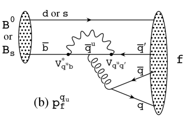
Figure 1: Feynman diagrams for (a) tree and (b) penguin amplitudes contributing to $B^{0}\to f$ or $B_{s}\to f$ via a $\bar{b}\to\bar{q}q\bar{q}^{\prime}$ quark-level process

The $B^{0}\to J/\psi K^{0}$ decay [Carter:1980hr, Bigi:1981qs] proceeds via the quark transition $\bar{b}\to\bar{c}c\bar{s}$. There are contributions from both tree ($t$) and penguin ($p^{q_{u}}$, where $q_{u}=u,c,t$ is the quark in the loop) diagrams (see fig:diags) which carry different weak phases:

$$A_{f}=\left(V^{\ast}_{cb}V_{cs}\right)t_{f}+\sum_{q_{u}=u,c,t}\left(V^{\ast}_{q_{u}b}V_{q_{u}s}\right)p^{q_{u}}_{f}\;.$$ (28)

(The distinction between tree and penguin contributions is a heuristic one, the separation by the operator that enters is more precise. For a detailed discussion of the more complete operator product approach, which also includes higher order QCD corrections, see, for example, Buchalla:1995vs.) Using CKM unitarity, these decay amplitudes can always be written in terms of just two CKM combinations:

$$A_{\psi K}=\left(V^{\ast}_{cb}V_{cs}\right)T_{\psi K}+\left(V^{\ast}_{ub}V_{us}\right)P^{u}_{\psi K},$$ (29)

where $T_{\psi K}=t_{\psi K}+p^{c}_{\psi K}-p^{t}_{\psi K}$ and $P^{u}_{\psi K}=p^{u}_{\psi K}-p^{t}_{\psi K}$. A subtlety arises in this decay that is related to the fact that ${B}^{0}\to J/\psi K^{0}$ and $\overline{B}^{0}\to J/\psi\overline{K}{}^{0}$. A common final state, $J/\psi K_{S}$, can be reached via $K^{0}$–$\overline{K}{}^{0}$ mixing. Consequently, the phase factor corresponding to neutral $K$ mixing, $e^{-i\phi_{K}}=(V^{*}_{cd}V_{cs})/(V_{cd}V^{*}_{cs})$, plays a role:

$$\frac{\overline{A}_{\psi K_{S}}}{A_{\psi K_{S}}}=-\frac{\left(V_{cb}V^{\ast}_{cs}\right)T_{\psi K}+\left(V_{ub}V^{\ast}_{us}\right)P^{u}_{\psi K}}{\left(V^{\ast}_{cb}V_{cs}\right)T_{\psi K}+\left(V^{\ast}_{ub}V_{us}\right)P^{u}_{\psi K}}\times\frac{V_{cd}^{\ast}V_{cs}}{V_{cd}V_{cs}^{\ast}}.$$ (30)

The crucial point is that, for $B\to J/\psi K_{S}$ and other $\bar{b}\to\bar{c}c\bar{s}$ processes, we can neglect the $P^{u}$ contribution to $A_{\psi K}$, in the SM, to an approximation that is better than one per cent:

$$|P^{u}_{\psi K}/T_{\psi K}|\times|V_{ub}/V_{cb}|\times|V_{us}/V_{cs}|\sim(\text{loop\ factor})\times 0.1\times 0.23\lesssim 0.005.$$ (31)

Thus, to an accuracy of better than one per cent,

$$\lambda_{\psi K_{S}}=\left(\frac{V_{tb}^{*}V_{td}}{V_{tb}V_{td}^{*}}\right)\left(\frac{V_{cb}V_{cd}^{*}}{V_{cb}^{*}V_{cd}}\right)=-e^{-2i\beta},$$ (32)

where $\beta$ is defined in abcangles, and consequently

$$S_{\psi K_{S}}=\sin 2\beta,\ \ \ C_{\psi K_{S}}=0\;.$$ (33)

(Below the per cent level, several effects modify this equation [Grossman:2002bu, Boos:2004xp, Li:2006vq, Gronau:2008cc].)

Exercise 3: Show that, if the $B\to\pi\pi$ decays were dominated by tree diagrams, then $S_{\pi\pi}=\sin 2\alpha$.

Exercise 4: Estimate the accuracy of the predictions $S_{\phi K_{S}}=\sin 2\beta$ and $C_{\phi K_{S}}=0$.

When we consider extensions of the SM, we still do not expect any significant new contribution to the tree level decay, $b\to c\bar{c}s$, beyond the SM $W$-mediated diagram. Thus the expression $\bar{A}_{\psi K_{S}}/A_{\psi K_{S}}=(V_{cb}V_{cd}^{*})/(V_{cb}^{*}V_{cd})$ remains valid, though the approximation of neglecting sub-dominant phases can be somewhat less accurate than smapprox. On the other hand, $M_{12}$, the $B^{0}$–$\overline{B}^{0}$ mixing amplitude, can in principle get large and even dominant contributions from new physics. We can parametrize the modification to the SM in terms of two parameters, $r_{d}^{2}$ signifying the change in magnitude, and $2\theta_{d}$ signifying the change in phase:

$$M_{12}=r_{d}^{2}\ e^{2i\theta_{d}}\ M_{12}^{\text}{SM}(\rho,\eta).$$ (34)

This leads to the following generalization of btopsik:

$$S_{\psi K_{S}}=\sin(2\beta+2\theta_{d}),\ \ \ C_{\psi K_{S}}=0\;.$$ (35)

The experimental measurements give the following ranges [hfag]:

$$S_{\psi K_{S}}=0.671\pm 0.024,\ \ \ C_{\psi K_{S}}=0.005\pm 0.019\;.$$ (36)

0.4.2 Self-consistency of the CKM assumption

The three-generation Standard Model has room for CP violation, through the KM phase in the quark mixing matrix. Yet, one would like to make sure that CP is indeed violated by the SM interactions, namely that $\sin\delta_{\text}{KM}\neq 0$. If we establish that this is the case, we would further like to know whether the SM contributions to CP violating observables are dominant. More quantitatively, we would like to put an upper bound on the ratio between the new physics and the SM contributions.

As a first step, one can assume that flavour-changing processes are fully described by the SM, and check the consistency of the various measurements with this assumption. There are four relevant mixing parameters, which can be taken to be the Wolfenstein parameters $\lambda$, $A$, $\rho$, and $\eta$ defined in wolpar. The values of $\lambda$ and $A$ are known rather accurately [Yao:2006px] from, respectively, $K\to\pi\ell\nu$ and $b\to c\ell\nu$ decays:

$$\lambda=0.2257\pm 0.0010,\ \ \ A=0.814\pm 0.022.$$ (37)

Then, one can express all the relevant observables as a function of the two remaining parameters, $\rho$ and $\eta$, and check whether there is a range in the $\rho$–$\eta$ plane that is consistent with all measurements. The list of observables includes the following:

• The rates of inclusive and exclusive charmless semileptonic $B$ decays depend on $|V_{ub}|^{2}\propto\rho^{2}+\eta^{2}$.

• The CP asymmetry in $B\to\psi K_{S}$, $S_{\psi K_{S}}=\sin 2\beta=\frac{2\eta(1-\rho)}{(1-\rho)^{2}+\eta^{2}}$.

• The rates of various $B\to DK$ decays depend on the phase $\gamma$, where $e^{i\gamma}=\frac{\rho+i\eta}{\rho^{2}+\eta^{2}}$.

• The rates of various $B\to\pi\pi,\rho\pi,\rho\rho$ decays depend on the phase $\alpha=\pi-\beta-\gamma$.

• The ratio between the mass splittings in the neutral $B$ and $B_{s}$ systems is sensitive to $|V_{td}/V_{ts}|^{2}=\lambda^{2}[(1-\rho)^{2}+\eta^{2}]$.

• The CP violation in $K\to\pi\pi$ decays, $\epsilon_{K}$, depends in a complicated way on $\rho$ and $\eta$.

The resulting constraints are shown in fg:UT.

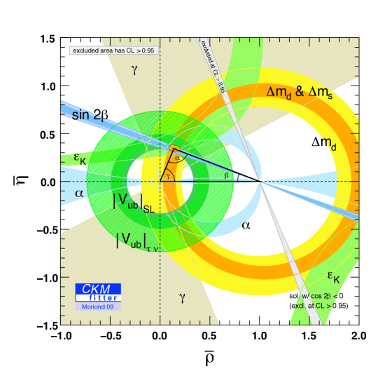
Figure 2: Allowed region in the $\rho$–$\eta$ plane. Superimposed are the individual constraints from charmless semileptonic $B$ decays ($|V_{ub}/V_{cb}|$), mass differences in the $B^{0}$ ($\Delta m_{d}$) and $B_{s}$ ($\Delta m_{s}$) neutral meson systems, and CP violation in $K\to\pi\pi$ ($\varepsilon_{K}$), $B\to\psi K$ ($\sin 2\beta$), $B\to\pi\pi,\rho\pi,\rho\rho$ ($\alpha$), and $B\to DK$ ($\gamma$). Taken from ckmfitter.

The consistency of the various constraints is impressive. In particular, the following ranges for $\rho$ and $\eta$ can account for all the measurements [Yao:2006px]:

$$\rho=0.135^{+0.031}_{-0.016},\ \ \ \eta=0.349\pm 0.017.$$ (38)

One can then make the following statement [Nir:2002gu]:
Very likely, CP violation in flavour-changing processes is dominated by the Kobayashi–Maskawa phase.

In the next two subsections, we explain how we can remove the phrase ‘very likely’ from this statement, and how we can quantify the KM dominance.

0.4.3 Is the Kobayashi–Maskawa mechanism at work?

In proving that the KM mechanism is at work, we assume that charged-current tree-level processes are dominated by the $W$-mediated SM diagrams (see, for example, Grossman:1997dd). This is a very plausible assumption. I am not aware of any viable well-motivated model where this assumption is not valid. Thus we can use all tree-level processes and fit them to $\rho$ and $\eta$, as we did before. The list of such processes includes the following:

1. Charmless semileptonic $B$-decays, $b\to u\ell\nu$, measure $R_{u}$ [see RbRt].

2. $B\to DK$ decays, which go through the quark transitions $b\to c\bar{u}s$ and $b\to u\bar{c}s$, measure the angle $\gamma$ [see abcangles].

3. $B\to\rho\rho$ decays (and, similarly, $B\to\pi\pi$ and $B\to\rho\pi$ decays) go through the quark transition $b\to u\bar{u}d$. With an isospin analysis, one can determine the relative phase between the tree decay amplitude and the mixing amplitude. By incorporating the measurement of $S_{\psi K_{S}}$, one can subtract the phase from the mixing amplitude, finally providing a measurement of the angle $\gamma$ [see abcangles].

In addition, we can use loop processes, but then we must allow for new physics contributions, in addition to the $(\rho,\eta)$-dependent SM contributions. Of course, if each such measurement adds a separate mode-dependent parameter, then we do not gain anything by using this information. However, there are a number of observables where the only relevant loop process is $B^{0}$–$\overline{B}{}^{0}$ mixing. The list includes $S_{\psi K_{S}}$, $\Delta m_{B}$, and the CP asymmetry in semileptonic $B$ decays:

$$S_{\psi K_{S}} =\sin(2\beta+2\theta_{d}),$$

$$\Delta m_{B} =r_{d}^{2}(\Delta m_{B})^{\text{SM}},$$

$$\mathcal{A}_{\text{SL}} =-\mathcal{R}e\left(\frac{\Gamma_{12}}{M_{12}}\right)^{\text{SM}}\frac{\sin 2\theta_{d}}{r_{d}^{2}}+\mathcal{I}m\left(\frac{\Gamma_{12}}{M_{12}}\right)^{\text{SM}}\frac{\cos 2\theta_{d}}{r_{d}^{2}}.$$ (39)

As explained above, such processes involve two new parameters [see derthed]. Since there are three relevant observables, we can further tighten the constraints in the $(\rho,\eta)$ plane. Similarly, one can use measurements related to $B_{s}$–$\overline{B}_{s}$ mixing. One gains three new observables at the cost of two new parameters (see, for example, Grossman:2006ce).

The results of such a fit, projected on the $\rho$–$\eta$ plane, can be seen in fig:re_tree. It gives [ckmfitter]

$$\eta=0.44^{+0.05}_{-0.23}\ \ (3\sigma).$$ (40)

[A similar analysis in Bona:2007vi obtains the $3\sigma$ range $(0.31$–$0.46)$.] It is clear that $\eta\neq 0$ is well established:
The Kobayashi–Maskawa mechanism of CP violation is at work.

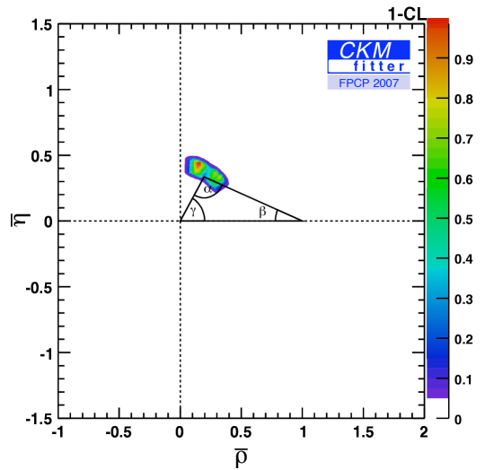
Figure 3: The allowed region in the $\rho$–$\eta$ plane, assuming that tree diagrams are dominated by the Standard Model [ckmfitter]

Another way to establish that CP is violated by the CKM matrix is to find, within the same procedure, the allowed range for $\sin 2\beta$ [Bona:2007vi]:

$$\sin 2\beta^{\text}{tree}=0.76\pm 0.04.$$ (41)

([b]ckmfitter finds $0.82^{+0.02}_{-0.13}$.) Thus, $\beta\neq 0$ is well established.

The consistency of the experimental results (36) with the SM predictions (33,41) means that the KM mechanism of CP violation dominates the observed CP violation. In the next subsection, we make this statement more quantitative.

0.4.4 How much can new physics contribute to $B^{0}$–$\overline{B}{}^{0}$ mixing?

All that we need to do in order to establish whether the SM dominates the observed CP violation, and to put an upper bound on the new physics contribution to $B^{0}$–$\overline{B}{}^{0}$ mixing, is to project the results of the fit performed in the previous subsection on the $r_{d}^{2}$–$2\theta_{d}$ plane. If we find that $\theta_{d}\ll\beta$, then the SM dominance in the observed CP violation will be established. The constraints are shown in fig:rdtd(a). Indeed, $\theta_{d}\ll\beta$.

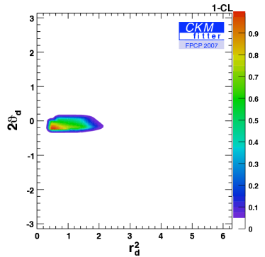
(a)  (b)

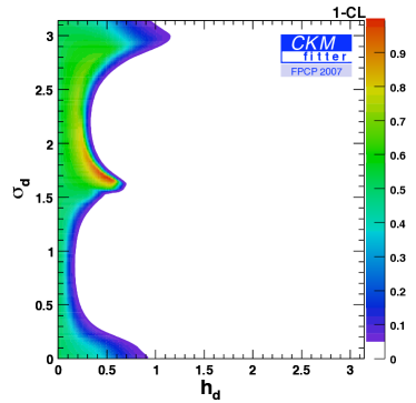
Figure 4: Constraints in the (a) $r_{d}^{2}$–$2\theta_{d}$ plane, and (b) $h_{d}$–$\sigma_{d}$ plane, assuming that new physics contributions to tree-level processes are negligible [ckmfitter]

An alternative way to present the data is to use the $h_{d},\sigma_{d}$ parametrization,

$$r_{d}^{2}e^{2i\theta_{d}}=1+h_{d}e^{2i\sigma_{d}}.$$ (42)

While the $r_{d},\theta_{d}$ parameters give the relation between the full mixing amplitude and the SM one, and are convenient to apply to the measurements, the $h_{d},\sigma_{d}$ parameters give the relation between the new physics and SM contributions, and are more convenient in testing theoretical models:

$$h_{d}e^{i\sigma_{d}}=\frac{M_{12}^{\text}{NP}}{M_{12}^{\text}{SM}}.$$ (43)

The constraints in the $h_{d}$–$\sigma_{d}$ plane are shown in fig:rdtd(b). We can make the following two statements:

1. A new physics contribution to the $B^{0}$–$\overline{B}^{0}$ mixing amplitude that carries a phase that is significantly different from the KM phase is constrained to lie below the $20$–$30$% level.

2. A new physics contribution to the $B^{0}$–$\overline{B}^{0}$ mixing amplitude which is aligned with the KM phase is constrained to be at most comparable to the CKM contribution.

One can reformulate these statements as follows:

1. The KM mechanism dominates CP violation in $B^{0}$–$\overline{B}^{0}$ mixing.

2. The CKM mechanism is a major player in $B^{0}$–$\overline{B}^{0}$ mixing.

0.5 The new physics flavour puzzle

It is clear that the Standard Model is not a complete theory of Nature:

1. It does not include gravity, and therefore it cannot be valid at energy scales above $m_{\text}{Planck}\sim 10^{19}\UGeV$.

2. It does not allow for neutrino masses, and therefore it cannot be valid at energy scales above $m_{\text}{seesaw}\sim 10^{15}\UGeV$.

3. The fine-tuning problem of the Higgs mass and the puzzle of dark matter suggest that the scale where the SM is replaced with a more fundamental theory is actually much lower, $\Lambda_{\text}{NP}\lesssim 1\UTeV$.

Given that the SM is only an effective low-energy theory, non-renormalizable terms must be added to $\mathcal{L}_{\text}{SM}$ of LagSM. These are terms of dimension higher than four in the fields which, therefore, have couplings that are inversely proportional to the scale of new physics $\Lambda_{\text}{NP}$. For example, the lowest-dimension non-renormalizable terms are dimension five:

$$-\mathcal{L}_{\text}{Yukawa}^{\text}{dim-5}=\frac{Z_{ij}^{\nu}}{\Lambda_{\text}{NP}}L_{Li}^{I}L_{Lj}^{I}\phi\phi+\text{h.c.}$$ (44)

These are the seesaw terms, leading to neutrino masses. We shall return to the topic of neutrino masses in sec:nu.

Exercise 5: How does the global symmetry breaking pattern (14) change when (44) is taken into account?

Exercise 6: What is the number of physical lepton flavour parameters in this case? Identify these parameters in the mass basis.

As concerns quark flavour physics, consider, for example, the following dimension-six, four-fermion, flavour-changing operators:

$$\mathcal{L}_{\Delta F=2}=\frac{z_{sd}}{\Lambda_{\text}{NP}^{2}}(\overline{d_{L}}\gamma_{\mu}s_{L})^{2}+\frac{z_{cu}}{\Lambda_{\text}{NP}^{2}}(\overline{c_{L}}\gamma_{\mu}u_{L})^{2}+\frac{z_{bd}}{\Lambda_{\text}{NP}^{2}}(\overline{d_{L}}\gamma_{\mu}b_{L})^{2}+\frac{z_{bs}}{\Lambda_{\text}{NP}^{2}}(\overline{s_{L}}\gamma_{\mu}b_{L})^{2}.$$ (45)

Each of these terms contributes to the mass splitting between the corresponding two neutral mesons. For example, the term $\mathcal{L}_{\Delta B=2}\propto(\overline{d_{L}}\gamma_{\mu}b_{L})^{2}$ contributes to $\Delta m_{B}$, the mass difference between the two neutral $B$-mesons. We use $M_{12}^{B}=\frac{1}{2m_{B}}\langle B^{0}|\mathcal{L}_{\Delta F=2}|\overline{B}^{0}\rangle$ and

$$\langle B^{0}|(\overline{d_{La}}\gamma^{\mu}b_{La})(\overline{d_{Lb}}\gamma_{\mu}b_{Lb})|\overline{B}^{0}\rangle=-\frac{1}{3}m_{B}^{2}f_{B}^{2}B_{B}.$$ (46)

Analogous expressions hold for the other neutral mesons. This leads to $\Delta m_{B}/m_{B}=2|M_{12}^{B}|/m_{B}\sim(|z_{bd}|/3)(f_{B}/\Lambda_{\text}{NP})^{2}$. Experiments give, for CP conserving observables (the experimental evidence for $\Delta m_{D}$ is at the $3\sigma$ level):

$$\Delta m_{K}/m_{K} \sim 7.0\times 10^{-15},$$

$$\Delta m_{D}/m_{D} \sim 8.7\times 10^{-15},$$

$$\Delta m_{B}/m_{B} \sim 6.3\times 10^{-14},$$

$$\Delta m_{B_{s}}/m_{B_{s}} \sim 2.1\times 10^{-12},$$ (47)

and for CP violating ones

$$\epsilon_{K} \sim 2.3\times 10^{-3},$$

$$A_{\Gamma}/y_{\rm CP} \mathrel{\hbox to0.0pt{\lower 4.0pt\hbox{\hskip 1.0pt$\sim$}\hss}\raise 1.0pt\hbox{$<$}} 0.2,$$

$$S_{\psi K_{S}} = 0.67\pm 0.02,$$

$$S_{\psi\phi} \mathrel{\hbox to0.0pt{\lower 4.0pt\hbox{\hskip 1.0pt$\sim$}\hss}\raise 1.0pt\hbox{$<$}} 1.$$ (48)

These measurements give then the following constraints:

$$\Lambda_{\rm NP}\mathrel{\hbox to0.0pt{\lower 4.0pt\hbox{\hskip 1.0pt$\sim$}\hss}\raise 1.0pt\hbox{$>$}}\cases{\sqrt{\hfil}}{z_{sd}}\ 1\times 10^{3}\ \textrm{TeV}&\Delta m_{K}\\ \sqrt{z_{cu}}\ 1\times 10^{3}\ \textrm{TeV}\Delta m_{D}\\ \sqrt{z_{bd}}\ 4\times 10^{2}\ \textrm{TeV}\Delta m_{B}\\ \sqrt{z_{bs}}\ 7\times 10^{1}\ \textrm{TeV}\Delta m_{B_{s}}$$ (49)

and, for maximal phases,

$$\Lambda_{\rm NP}\mathrel{\hbox to0.0pt{\lower 4.0pt\hbox{\hskip 1.0pt$\sim$}\hss}\raise 1.0pt\hbox{$>$}}\cases{\sqrt{\hfil}}{z_{sd}}\ 2\times 10^{4}\ \textrm{TeV}&\epsilon_{K}\\ \sqrt{z_{cu}}\ 3\times 10^{3}\ \textrm{TeV}A_{\Gamma}\\ \sqrt{z_{bd}}\ 8\times 10^{2}\ \textrm{TeV}S_{\psi K}\\ \sqrt{z_{bs}}\ 7\times 10^{1}\ \textrm{TeV}S_{\psi\phi}$$ (50)

If the new physics has a generic flavour structure, that is $z_{ij}={\cal O}(1)$, then its scale must be above $10^{3}$–$10^{4}$ TeV (or, if the leading contributions involve electroweak loops, above $10^{2}$–$10^{3}$ TeV).

If indeed $\Lambda_{\rm NP}\gg\textrm{TeV}$, it means that we have misinterpreted the hints from the fine-tuning problem and the dark matter puzzle. There is, however, another way to look at these constraints:

$$z_{sd} \mathrel{\hbox to0.0pt{\lower 4.0pt\hbox{\hskip 1.0pt$\sim$}\hss}\raise 1.0pt\hbox{$<$}} 8\times 10^{-7}\ (\Lambda_{\rm NP}/\textrm{TeV})^{2},$$

$$z_{cu} \mathrel{\hbox to0.0pt{\lower 4.0pt\hbox{\hskip 1.0pt$\sim$}\hss}\raise 1.0pt\hbox{$<$}} 5\times 10^{-7}\ (\Lambda_{\rm NP}/\textrm{TeV})^{2},$$

$$z_{bd} \mathrel{\hbox to0.0pt{\lower 4.0pt\hbox{\hskip 1.0pt$\sim$}\hss}\raise 1.0pt\hbox{$<$}} 5\times 10^{-6}\ (\Lambda_{\rm NP}/\textrm{TeV})^{2},$$

$$z_{bs} \mathrel{\hbox to0.0pt{\lower 4.0pt\hbox{\hskip 1.0pt$\sim$}\hss}\raise 1.0pt\hbox{$<$}} 2\times 10^{-4}\ (\Lambda_{\rm NP}/\textrm{TeV})^{2},$$ (51)

$$z_{sd}^{I} \mathrel{\hbox to0.0pt{\lower 4.0pt\hbox{\hskip 1.0pt$\sim$}\hss}\raise 1.0pt\hbox{$<$}} 6\times 10^{-9}\ (\Lambda_{\rm NP}/\textrm{TeV})^{2},$$

$$z_{cu}^{I} \mathrel{\hbox to0.0pt{\lower 4.0pt\hbox{\hskip 1.0pt$\sim$}\hss}\raise 1.0pt\hbox{$<$}} 1\times 10^{-7}\ (\Lambda_{\rm NP}/\textrm{TeV})^{2},$$

$$z_{bd}^{I} \mathrel{\hbox to0.0pt{\lower 4.0pt\hbox{\hskip 1.0pt$\sim$}\hss}\raise 1.0pt\hbox{$<$}} 1\times 10^{-6}\ (\Lambda_{\rm NP}/\textrm{TeV})^{2},$$

$$z_{bs}^{I} \mathrel{\hbox to0.0pt{\lower 4.0pt\hbox{\hskip 1.0pt$\sim$}\hss}\raise 1.0pt\hbox{$<$}} 2\times 10^{-4}\ (\Lambda_{\rm NP}/\textrm{TeV})^{2}.$$ (52)

It could be that the scale of new physics is of order TeV, but its flavour structure is far from generic.

One can use that language of effective operators also for the SM, integrating out all particles significantly heavier than the neutral mesons (that is, the top, the Higgs, and the weak gauge bosons). Thus the scale is $\Lambda_{\text}{SM}\sim m_{W}$. Since the leading contributions to neutral meson mixings come from box diagrams, the $z_{ij}$ coefficients are suppressed by $\alpha_{2}^{2}$. To identify the relevant flavour suppression factor, one can employ the spurion formalism. For example, the flavour transition that is relevant to $B^{0}$–$\overline{B}{}^{0}$ mixing involves $\overline{d_{L}}b_{L}$ which transforms as $(8,1,1)_{SU(3)_{q}^{3}}$. The leading contribution must then be proportional to $(Y^{u}Y^{u\dagger})_{13}\propto y_{t}^{2}V_{tb}V_{td}^{*}$. Indeed, an explicit calculation (using VIA for the matrix element and neglecting QCD corrections) gives

$$\frac{2M_{12}^{B}}{m_{B}}\approx-\frac{\alpha_{2}^{2}}{12}\frac{f_{B}^{2}}{m_{W}^{2}}S_{0}(x_{t})(V_{tb}V_{td}^{*})^{2},$$ (53)

where $x_{i}=m_{i}^{2}/m_{W}^{2}$ and

$$S_{0}(x)=\frac{x}{(1-x)^{2}}\left[1-\frac{11x}{4}+\frac{x^{2}}{4}-\frac{3x^{2}\ln x}{2(1-x)}\right].$$ (54)

Similar spurion analyses, or explicit calculations, allow us to extract the weak and flavour suppression factors that apply in the SM: