Towards a fully consistent Milky Way disc model - II. The local disc model and SDSS data of the NGP region
Abstract
We have used the self-consistent vertical disc models of the solar neighbourhood presented in Just & Jahreiss (2010), which are based on different star formation histories (SFR) and fit the local kinematics of main sequence stars equally well, to predict star counts towards the North Galactic Pole (NGP). We combined these four different models with the local main sequence in the filter system of the SDSS and predicted the star counts in the NGP field with . All models fit the Hess diagrams in the F–K dwarf regime better than percent and the star number densities in the solar neighbourhood are consistent with the observed values. The analysis shows that model A is clearly preferred with systematic deviations of a few percent only. The SFR of model A is characterised by a maximum at an age of 10 Gyr and a decline by a factor of four to the present day value of 1.4 /pc2/Gyr. The thick disc can be modelled very well by an old isothermal simple stellar population. The density profile can be approximated by a sech function. We found a power law index and a scale height pc corresponding to a vertical velocity dispersion of km/s. About 6 percent of the stars in the solar neighbourhood are thick disc stars.
keywords:
Galaxy: solar neighbourhood – Galaxy: disc – Galaxy: structure – Galaxy: evolution – Galaxy: stellar content – Galaxy: kinematics and dynamics1 Introduction
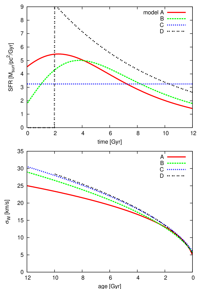
In Just & Jahreiss (2010) (hereafter Paper I) a self-consistent model of the vertical structure of the Milky Way disc in the solar neighbourhood was presented. The model is based on the star formation history (SFR), the age velocity dispersion relation (AVR), and a simple chemical enrichment model. The vertical density profiles of the stellar sub-populations are self-consistently calculated in the total gravitational potential of stars including the contribution of the gas component and the dark matter halo. The input parameters are selected and optimised to reproduce the velocity distribution functions for the vertical velocity component along the main sequence (MS). It turned out that for each SFR the range of fitting AVRs is very small. On the other hand the SFR is not well determined by the local kinematics only. Therefore we discussed in Paper I four different SFRs with similar values to cover the range of possible functional shapes (models A, B, C, and D). The overall range of best fitting AVRs is still well restricted. Due to the different age distributions and consequently different relative contributions of the sub-populations as function of scale height the vertical density profiles of MS stars differ significantly at large distances above the Galactic mid-plane.
A combination of the local model with number densities of MS stars in the solar neighbourhood allows predictions of star counts at high Galactic latitude. Therefore we can use star counts of large surveys for an independent test of the local model. As a new additional result we expect to find restrictions on the SFR. As local normalisation along the MS we use Hipparcos stars complemented by the Catalogue of Nearby Stars (CNS4) at the faint end (Jahreiß & Wielen, 1997). The model predictions will be compared to the North Galactic Pole (NGP) data of the Sloan Digital Sky Survey (SDSS), which has collected at present the largest and most homogeneous database comprising about stellar objects in the Milky Way (Gunn et al., 1998; Abazajian et al., 2009). The SDSS photometry is in the filter system. Despite the enormous wealth of information that the SDSS database provides in the filter system, the majority of current observational and theoretical knowledge of resolved stellar populations is based largely on the Johnson-Kron-Cousins photometric system and some other systems such as the Strömgren, DDO, Vilnius, and Geneva systems. To overcome this difficulty, we use an empirical transformation of the nearby MS star photometry into the system (Just & Jahreiss, 2008). For each theoretical model we derive a best fit solution for the full Hess diagrams in , which quantify the number density distributions in the colour magnitude diagram (CMD).
The paper is organised as follows. In Sect. 2 we describe the data selection, in Sect. 3 important properties of the theoretical models are presented, in Sect. 4 the local normalisation is discussed, in Sect. 5 we present the best fit procedure, in Sect. 6 we discuss the results, and in Sect. 7 we draw some conclusions.
2 SDSS Data
The Sloan Digital Sky Survey (SDSS) is an imaging and spectroscopic survey (York et al., 2000) that has since 1998 with its m dedicated telescope mapped more than a quarter of the sky (Gunn et al., 1998). Photometric sky coverage of the SDSS Data Release 7 (DR7) amounts to , including a large contiguous area around the NGP (Adelman-McCarthy et al., 2008; Abazajian et al., 2009).
Smith et al. (2002) defined the photometric system on 158 standard stars, a subset of standard stars from Landolt (1992), using the USNO-1.0m telescope. Unfortunately, the photometric system of the 2.5m SDSS telescope, denoted as , slightly differs from the one (Abazajian et al., 2003). Moreover, the SDSS standards are too bright and saturate in the 2.5m SDSS telescope during its normal operational mode. These inconveniences have been resolved by using fainter secondary standards scattered throughout the SDSS survey area and by using simple linear transformation equations between the two photometric sets (Tucker et al., 2006). The nightly photometry obtained by the SDSS 2.5m telescope can be thus calibrated to the native system with magnitude zero points accurate on the AB system to within a few percent.
Imaging data are produced simultaneously in the five photometric bands, namely , , , , and (Fukugita et al., 1996; Gunn et al., 2006; Smith et al., 2002; Hogg et al., 2001). The images are automatically processed through specialised pipelines (Lupton, Gunn, & Szalay, 1999; Lupton et al., 2001; Stoughton et al., 2002; Pier et al., 2003; Tucker et al., 2006) producing corrected images, object catalogues, astrometric solutions, calibrated fluxes and many other data products. SDSS photometry is homogeneous and deep (), repeatable to mag (Ivezić et al., 2003) and with a zero-point uncertainty of (Abazajian et al., 2004; Ivezić et al., 2004). In DR7 a homogeneous photometry over the full sky coverage was established at the 1 percent level in and 2 percent in in a process called ubercalibration (Padmanabhan, N., et al., 2008).
We have limited our analysis to the stars in the magnitude range 111Magnitude limits applied to the dereddenend magnitudes.
We applied the standard dereddening of the data based on the extinction map of
Schlegel et al. (1998) as given in the data base of SDSS..
For brighter stars the CCD camera of the SDSS telescope saturates.
At the faint end we wanted to completely avoid the problems in the galaxy-star
separation and we set a conservative magnitude limit for this purpose. The SDSS
photometric data contain also quality flags for each object to aid in the
selection of ”good” measurements222See the following link for the clean
photometry prescriptions:
http://cas.sdss.org/dr7/en/help/docs/realquery.asp#flags.. We have
carefully analysed the appearance of these photometric flags with respect to the
object brightness. We concluded that the problematic flags relate mostly to the
stars fainter than our faint magnitude limit. Many of these flags are also
tightly correlated with the magnitude measurement error. To make our stellar
samples as complete as possible we have finally applied only one ”cleaning”
criterion, i.e. we have rejected all the measurements with reported magnitude
error larger than in or in filter, which typically accounted
for 1 percent or even less of the total star counts. It is also necessary to
mention that the typical magnitude error in the chosen magnitude range is much
smaller than the applied magnitude error limit.
We selected the colour range with a symmetric bin size of mag. This range covers the MS down to K dwarfs, where the local normalisation is reliable. In order to test the predictions from the vertical structure of the local disc model (Paper I) with the available SDSS photometric data we have selected a field at the NGP. The field should not reach too low galactic latitude in order to avoid projection effects and a dependence of the star counts on the radial properties of the disc model. At the same time the field should be as large as possible in order to reduce the Poisson noise of the star counts. We have chosen a NGP field with Galactic latitudes and an area of . In magnitude we use a resolution of mag, but for the fitting procedure we applied a car-box smoothing of 0.1, 0.2, and 0.5 mag, where the last value is our standard case. The resolution in colour is mag. The Hess diagram of the data is shown in the bottom panel of figure 4.
In order to avoid confusion of observational errors in the SEGUE data and uncertainties of the model predictions we compare dereddened number counts in the colour – apparent magnitude plane.
3 The Milky Way Model
We use the self-consistent local model of the thin and thick disc described in detail in Paper I and add a simple stellar halo component. In this section we report the necessary features to understand the procedure applied here. The disc model relies on the kinematics of MS stars in the solar neighbourhood measured by volume complete local samples of stars combining Hipparcos stars and faint stars of the CNS4. The properties of the model depend on the total stellar mass density in the solar neighbourhood and only weakly on the adopted Initial Mass Function (IMF). It is independent of star counts at large distances.
The thin disc model at the solar radius is based on a pair (SFR,AVR) as input functions, which determines the age distribution and the velocity distribution functions of the stellar sub-populations. The vertical density profiles are calculated self-consistently in dynamical equilibrium in the total gravitational potential of stars, gas and dark matter halo. The chemical enrichment is also included for the determination of MS lifetimes, colour indices and luminosities from Padova population synthesis models. For each pair of functions (SFR,AVR) the local disc model provides a unique connection of local star counts and the number density of stars above the galactic plane with no additional free parameters. In Paper I we compared four different models A, B, C, D which all yield similar best fit values. The SFR and AVR of these models are plotted in figure 1.
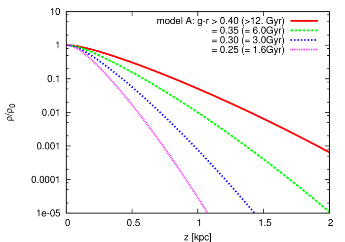
The density profile of MS stars at a given colour index is characterised by the MS lifetime of the stars. It is composed of a series of density profiles of coeval stars according to the SFR up to the lifetime. The top panel of figure 2 shows the normalised density profiles of model A for the relevant colour index range in . Bluer thin disc stars are too bright to be visible in SDSS at high Galactic latitude.
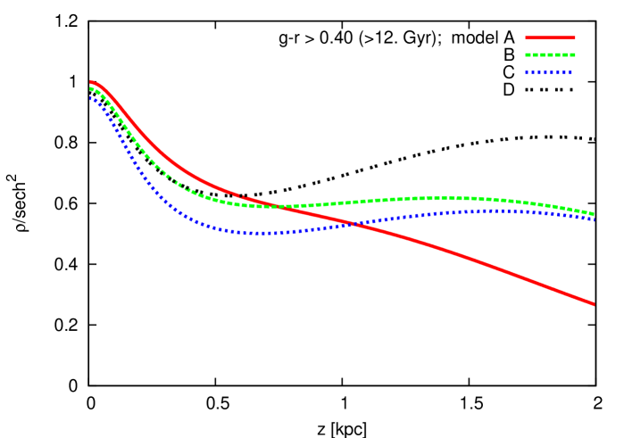
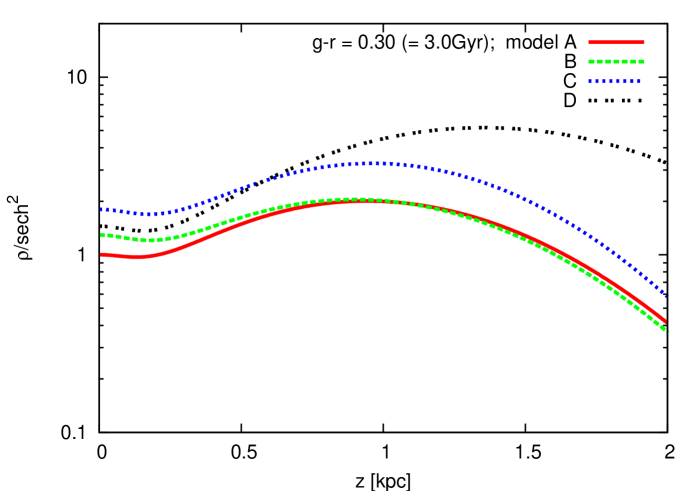
The lower panels of figure 2 show the density profiles of models A – D divided by a profile with exponential scale height for two colour (MS lifetime) bins. For both lifetimes we use the corresponding exponential scale height of model A, i.e. =270, 108 pc respectively. The middle panel is in linear scale, whereas the lower panel for stars with shorter lifetime is in log-scale. The deviations from a sech2-profile of model A are significant for all lifetimes, because the populations are not isothermal and their spatial distribution is influenced by the gravitational potential of all other components. For younger populations the deviations are much stronger than for older populations. Between the different models the differences exceed a factor of two. Models B–D with a lower fraction of stars older than 10 Gyr require larger velocity dispersions of the old thin disc populations (see figure 1). This leads to shallower density profiles at kpc. All profiles are based on a Scalo IMF. The differences at the mid-plane can be corrected by adjusting the IMF, which will be done implicitly by fitting the local normalisation (see below). In any case large differences of star counts as function of distance (apparent magnitude) remain.
In each colour bin the density profile is characterised by the MS lifetime. According to Paper I and Just & Jahreiss (2008) we use for the bins =0.15, 0.2, 0.25 the lifetime 1.2, 1.4, 1.6 Gyr, respectively. In the colour bins =0.3, 0.35, 0.4 we include the contribution of turnoff stars and use lifetime ranges 2.4–3.2, 4.0–6.2 and 8.2–12 Gyr, respectively. For all colours 0.45 the lifetime is larger than 12 Gyr leading to the same density profile.
An isothermal thick disc component is self-consistently included in the local model. We have shown in Paper I that it can be well fitted by a
| (1) |
law with local density and exponential scale height . Since the influence of the thick disc on the total gravitational potential is very small, the thick disc parameters can be varied in a large range with negligible influence on and the thin disc structure. From the Jeans equation it follows that and are both proportional to the square of the velocity dispersion of the thick disc in a given gravitational potential. As a consequence we find
| (2) |
which we use to maintain dynamical equilibrium, when changing the thick disc parameters. For the stellar population of the thick disc we adopt a simple population with an age of 12 Gyr and metallicity [Fe/H]=-0.7.
We include a simple stellar halo described by a flattened power law distribution
| (3) |
with flattening and local normalisation . For the distance of the Sun to the Galactic centre we adopt kpc. Since we are looking only to one line of sight and to distances not large compared to , the parameters and are strongly degenerated. A stronger flattening requires a shallower slope in order to reproduce similar stellar densities at a distance of kpc. One choice to get minimum values is and , which we fix for the further investigations.
For the calculation of star counts we use the density profiles of each component at distance along the line of sight pointing to the Galactic coordinate position normalised at the solar position
| (4) | |||||
| (5) |
For the thin disc the density profile depends also on colour . The vertical offset pc of the solar position can be easily included but is negligible for high Galactic latitude fields. The density distributions of thin and thick disc can be extended in the radial direction by an exponential profile, if necessary. The normalised density profiles of each component are transformed to number density profiles by multiplying with the local number densities determined from the HRD in the solar neighbourhood.
4 Local Normalisation
The Galaxy model described in the last section must be complemented by the local stellar number density of each component . In general the full HRD of a volume complete sample should be used. Since most of the modelled CMD is dominated to more than 95 percent by MS stars, we restrict the star count predictions to MS stars including a correction for turnoff stars. Only at the bright red corner of the CMD the K giants of thick disc and halo contribute significantly.
The stellar content in the solar neighbourhood is quantified by the number of MS stars with
| (6) |
in a sphere of 25 pc radius with volume pc3. Here the contributions of thin disc, thick disc, and halo are denoted by the indices s, t, and h, respectively. In Just & Jahreiss (2008) absolute magnitudes and colours of the mean MS in the filter system were determined based on different transformation formulae available in the literature. We use that mean MS for the thin disc, because the influence of thick disc and halo stars in the solar neighbourhood is negligible.
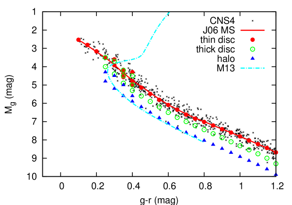
In figure 3 we show for the thin disc based on the transformation J06 (Jordi et al., 2006). The black crosses denote the MS stars of the CNS4 which are the basis for the determination of the mean MS. Each red full circle along the MS denotes a data point, where is a free fitting parameter. The locus of the MS corresponds to a slightly sub-solar mean metallicity and is consistent with the fiducial sequences of the open clusters M 67 ([Fe/H]=0) and NGC 2420 ([Fe/H]=-0.37) of An et al. (2008). Since the mean metallicity of the thin disc population decreases with increasing distance from the mid-plane, a correction to the mean luminosity in each colour bin is necessary. We use a simple analytic approximation
| (7) |
which is consistent with the determination of Ivezić et al. (2008) for the luminosity of thin disc MS stars.
For the thick disc we use an interpolated MS with corresponding to an old population with metallicity [Fe/H] (green open circles in figure 3).
The stellar halo is represented by corresponding to an old population with metallicity [Fe/H] (blue triangles in figure 3), where we used the fiducial sequence of M15 (An et al., 2008) with an extrapolation to the faint end.
In the turnoff regime of F stars we split the MS luminosity into two or three points with different luminosities in order to include the brighter turnoff stars. The total number of thin disc, thick disc and halo should add up to the observed total number of MS stars , which were also determined in Just & Jahreiss (2008) (histogram in figure 8). We treat the local number densities of the components as free fitting parameters and then compare the results of the best-fitting model to the observed stellar content in the solar neighbourhood.
The predicted Hess diagrams, i.e. the star counts in the CMD per bin, in a cone with cross section pointing to the Galactic coordinate position are calculated by adding up the contributions of each component along the line of sight. The contribution of each component by a volume element at distance , using , is given by
Adding up the contributions of all components along the line of sight yields the predicted number in each bin of the Hess diagram. In the next step the values are smoothed in the same way as the SDSS data. The star numbers in the Hess diagrams are normalised to 1 deg2 at the sky (second line of equation 4). In we need to distinguish between the resolution , the smoothing and the normalisation. All Hess diagrams are normalised to 0.1 mag in and 1.0 mag in .

5 Fitting procedure
The best-fit procedure in the colour bins are independent of each other. In each colour bin the contribution of thin disc, thick disc, and stellar halo to the local star counts in are quantified by the free parameters , and , respectively. The arguments are dropped here for simplicity. We use the nonlinear Levenberg-Marquard algorithm (Press et al., 1992) to minimise in each colour bin
| (9) |
in log-scale with Poisson noise for the statistical weights . In linear scale the regions with maximum density would dominate the value resulting in an unsatisfactory overall fit. The are derived from normalised values and have to be corrected by the area in units of deg2 and the bin size in units of . Due to the smoothing in over data points is the average over all subsets of independent bins with shifted by . In each colour bin the degrees of freedom for the independent bin sets depend on the fit regime in , the bin size and the number of fitting parameters. We derive the mean reduced by adding up the normalised values
| (10) |
In order to get reliable fits we restrict the colour range of the fitting regime. For the thin disc we fix for , since the main contribution falls outside the bright limit mag. For the halo we extrapolate for , since the main contribution falls outside the faint limit mag. Additionally the part of the CMD, which we use to minimise is restricted dependent on the aspect of investigation.
6 Results
We discuss first the construction of the Hess diagrams and compare the best fit results of models A – D. Then we investigate the dependence of the fitting result on the fitting regime and the MS properties for model A.
6.1 Hess diagram fitting
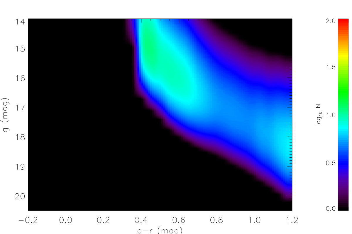
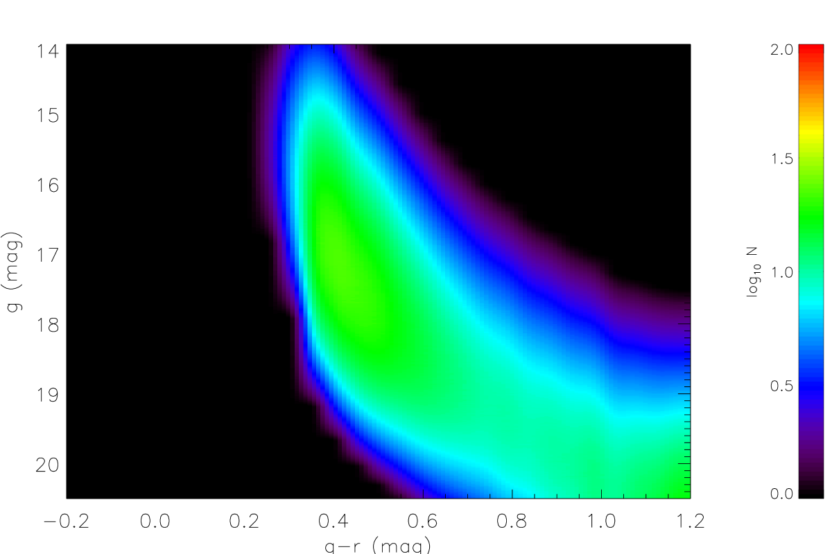
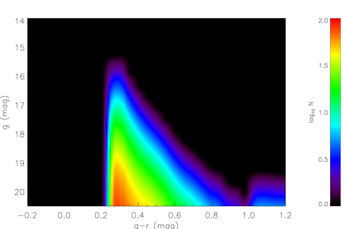
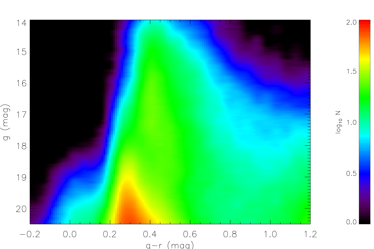
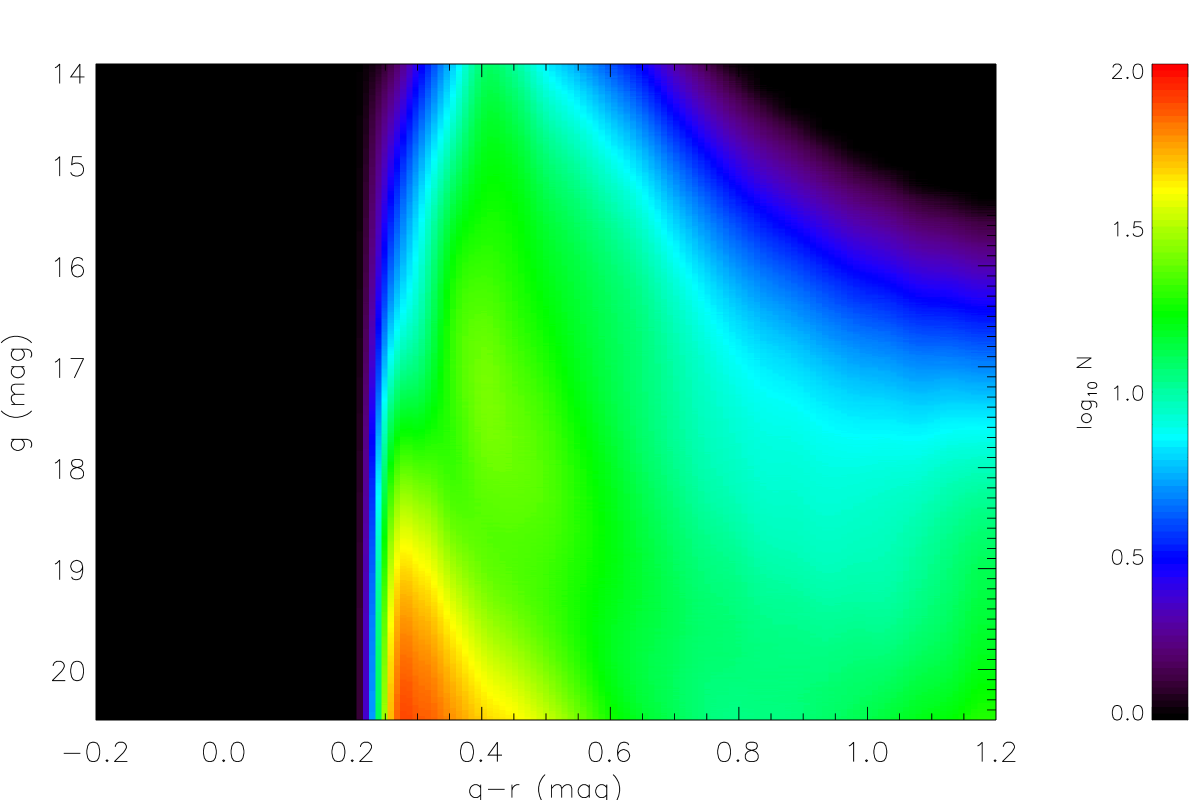
The bottom panel of figure 4 shows the Hess diagram of the NGP data with a total of 276,180 stellar objects. Star number densities normalised to 0.1 mag1.0 mag in and 1 deg2 are colour coded in log-scale ranging from 1…100 (purple …red). The plots are smoothed in colour and magnitude in boxes in steps of 0.01 mag with box size 0.05 mag0.5 mag (in the fitting procedure the colour bins are not smoothed). Most of the Hess diagram is strongly dominated by MS stars. Exceptions are turn-off stars in the colour range 0.3–0.4 and red giants of thick disc and/or halo in the upper right corner. The nature of the faint very blue objects with 0.15 is unclear (miss-identified extragalactic sources, White Dwarfs, halo BHB stars, …).


The three top panels of figure 4 show the contributions of the different components to the full Hess diagram for model A. There is a significant overlap of thin/thick disc, as well as thick disc/halo. Therefore the stellar halo must be included to determine the thick disc properties and the thick disc is needed to fix the thin disc parameters. The second last plot shows the sum of all components for model A.
For the comparison of disc models A – D we restrict the colour range to mag in order to avoid the F turn-off regime, which may be improperly modelled and thus dominate the total . The magnitude range is mag for safely excluding a contribution of saturated stars brighter than 14.25 mag in the brightest bins and a significant contamination by misidentified extragalactic sources at the faint end. In all models the thick disc parameters are varied according to equation 2 to find the minimum value. The parameters of the best fits are collected in the first four rows of table 1. In the model names there are tokens for the local normalisation (-J06 for Jordi et al. (2006), -R06 for Rodgers et al. (2006), -C08 for Chonis & Gaskell (2008)) and the smoothing (-01, -02, -05, respectively) attached. For the first block ’-r’ is attached for the reduced fit regime.
| model | ||||||
| A-J06-05-r | 0.5 | 2.59 | 739 | 800 | 1.16 | 45.3 |
| B-J06-05-r | 0.5 | 3.75 | 748 | 880 | 1.07 | 47.4 |
| C-J06-05-r | 0.5 | 3.84 | 811 | 885 | 1.23 | 51.2 |
| D-J06-05-r | 0.5 | 5.64 | 709 | 930 | 0.99 | 48.0 |
| A-R06-05-r | 0.5 | 2.61 | 715 | 800 | 1.16 | 45.3 |
| A-C08-05-r | 0.5 | 2.60 | 733 | 800 | 1.16 | 45.3 |
| A-J06-05 | 0.5 | 4.50 | 762 | 800 | 1.16 | 45.3 |
| A-R06-05 | 0.5 | 4.31 | 710 | 800 | 1.16 | 45.3 |
| A-C08-05 | 0.5 | 5.09 | 752 | 800 | 1.16 | 45.3 |
| A-C08-02 | 0.2 | 2.53 | 750 | 800 | 1.16 | 45.3 |
| A-C08-01 | 0.1 | 1.84 | 753 | 800 | 1.16 | 45.3 |
Note. The models are named by the disc model A – D followed by the local normalisation and the smoothing . For the first block ’r’ is added for the reduced fit regime. The observed number of stars range from (with R06) to (with C08).
6.2 The star formation history
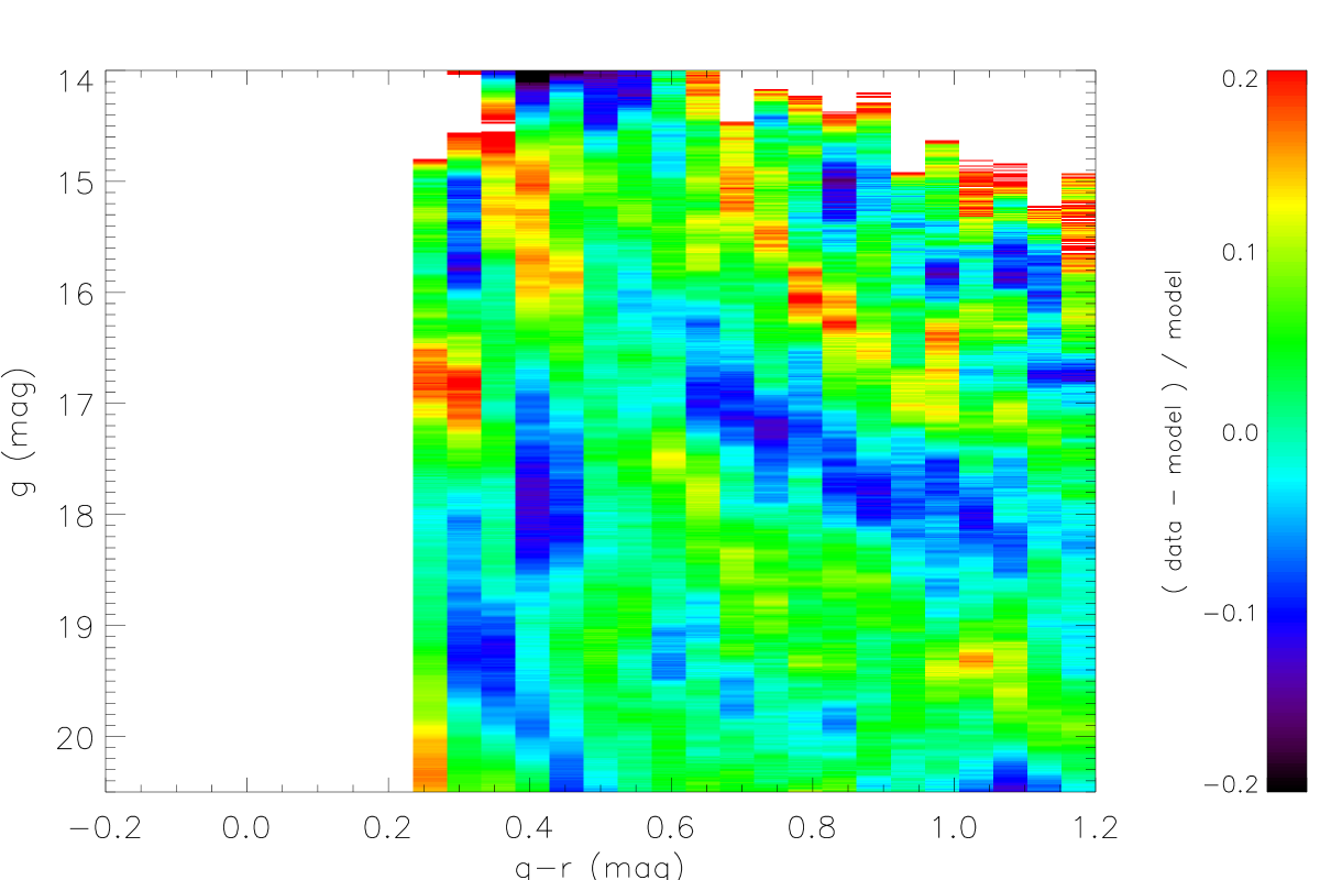
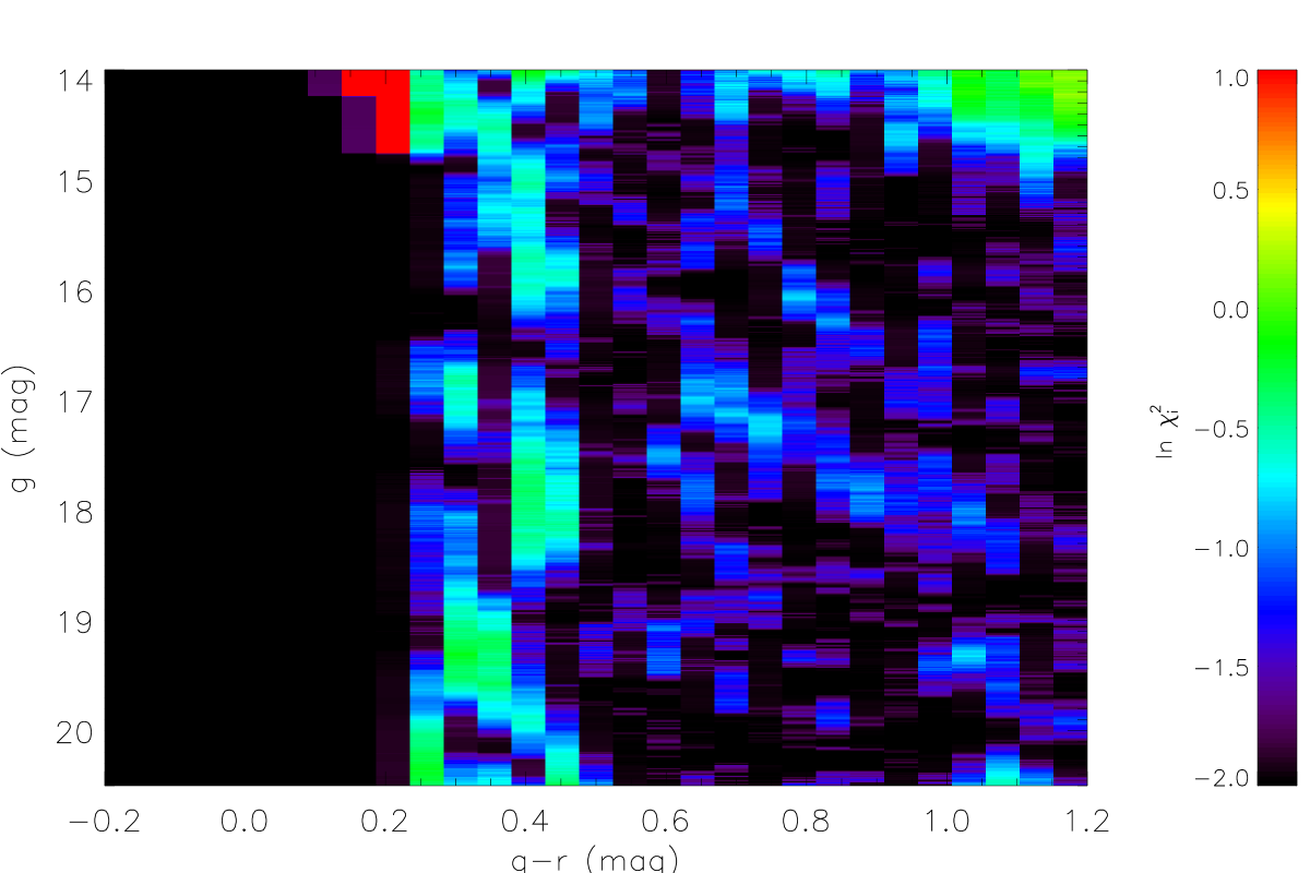
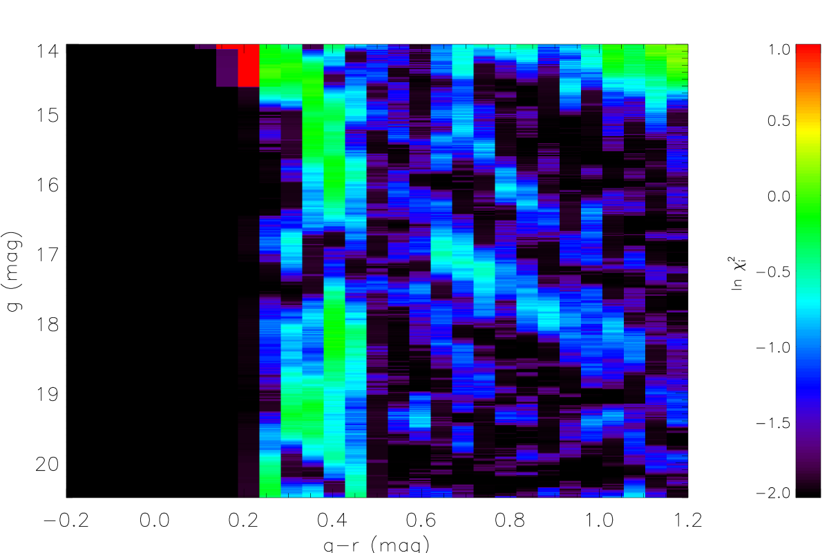
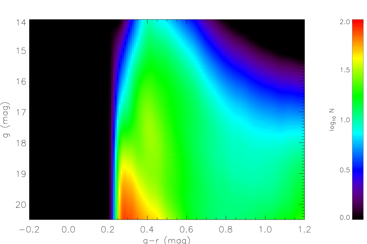
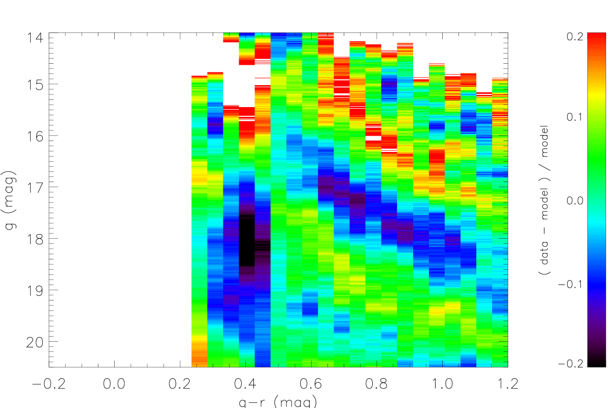
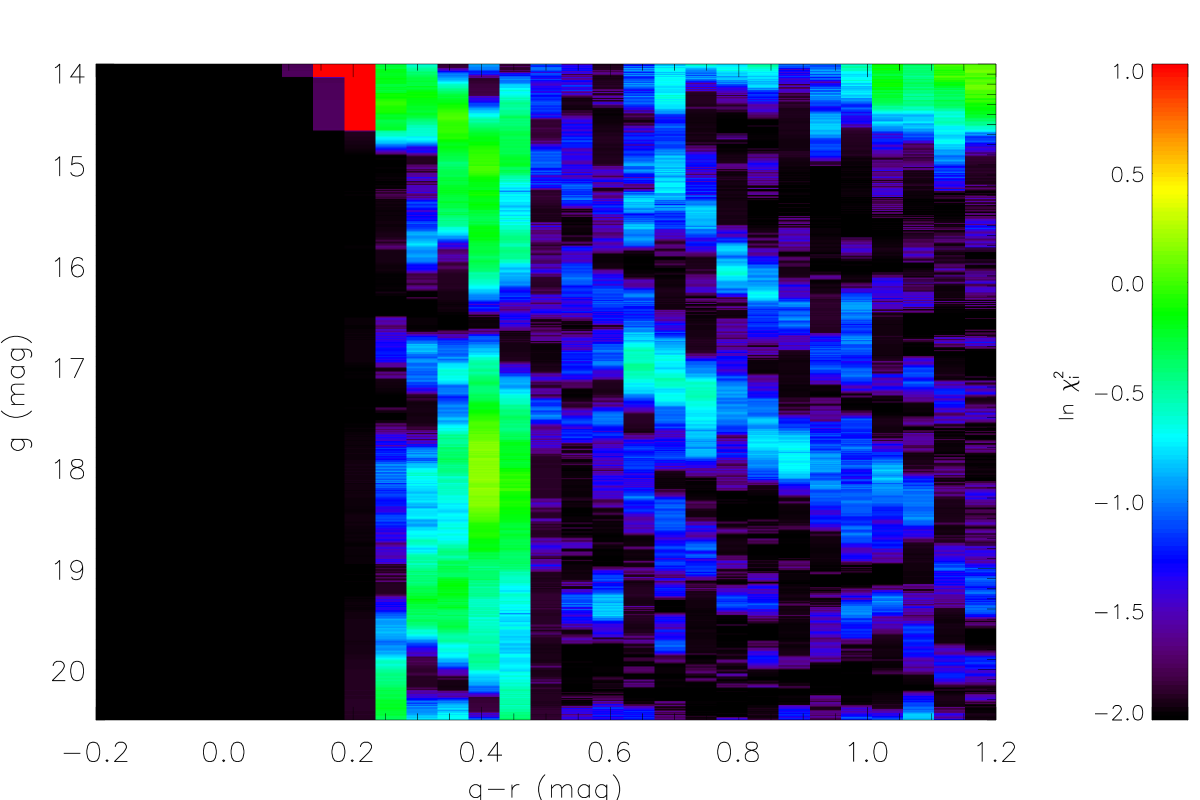
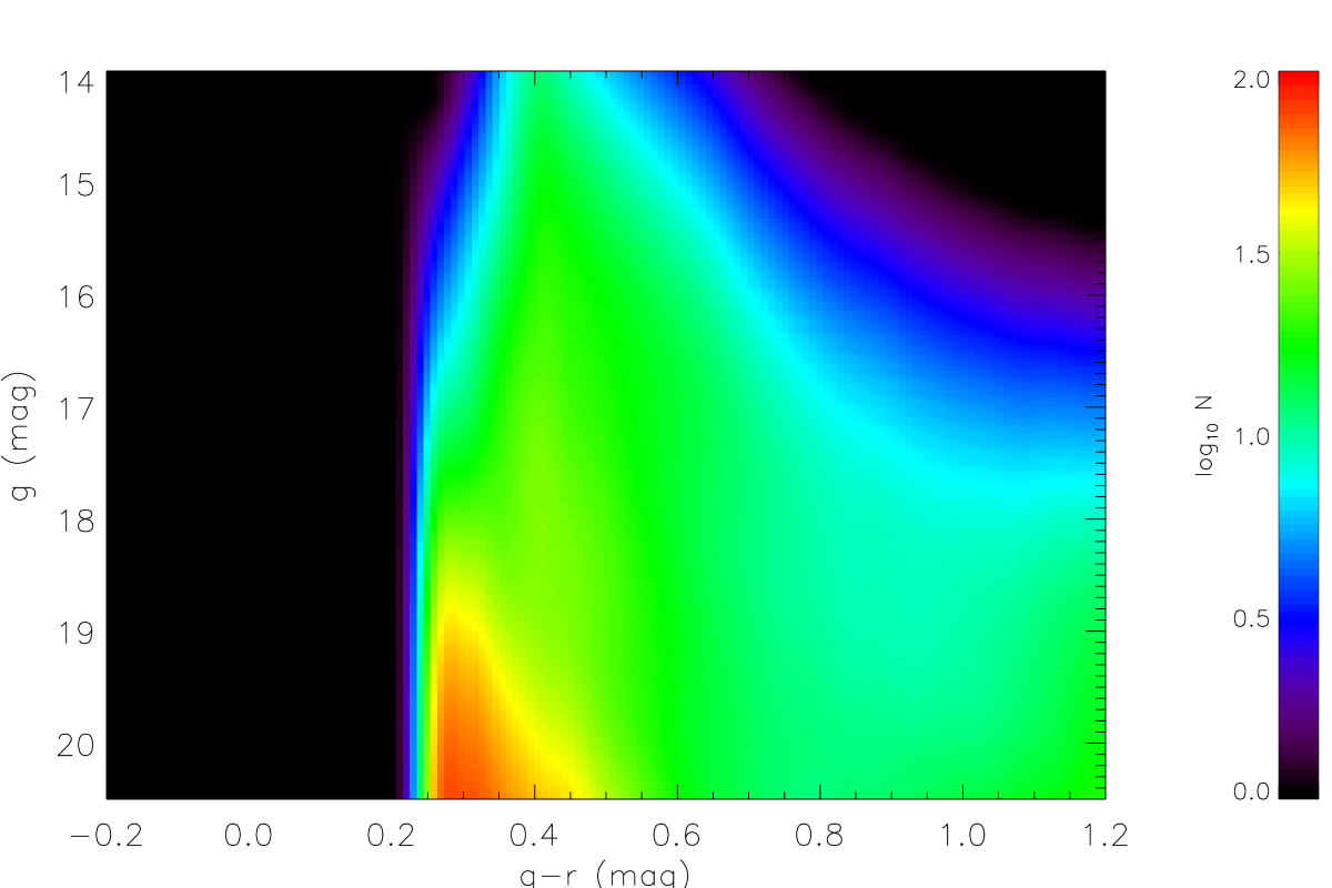
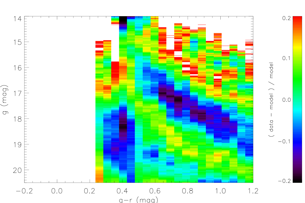
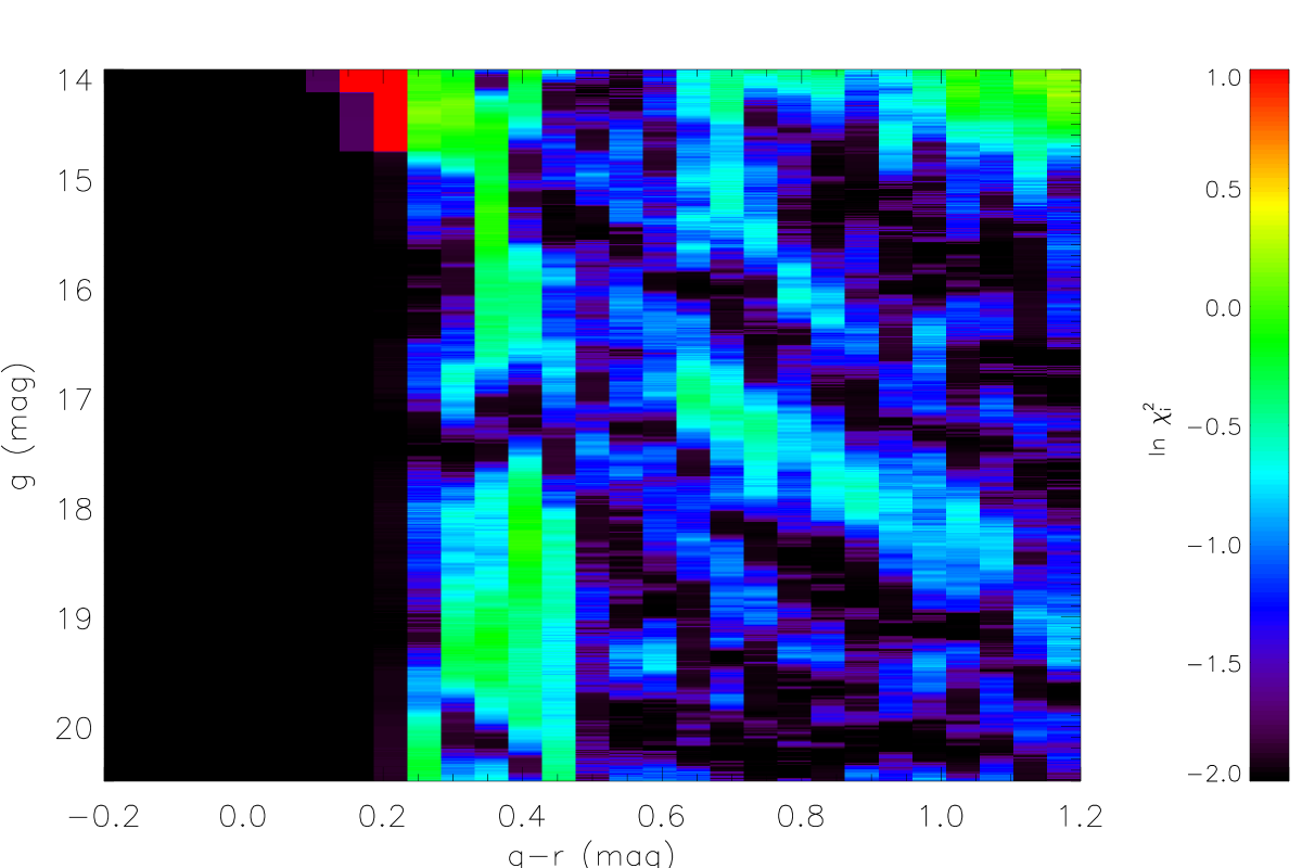
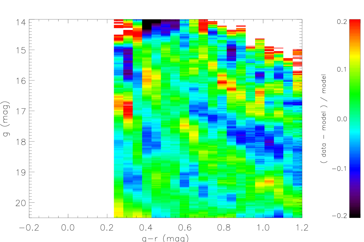
The thin disc models A – D have very different SFRs leading to different star count predictions. In each model we optimised the thick disc scale height and power law index according to equation 2 starting from a self-consistent isothermal model. In figure 5 the Hess diagrams of the models are presented in the left column (A – D: top – bottom). The middle column shows the relative differences (data-model)/model, where the coloured region covers the range -20 percent (purple) to +20 percent (red) in linear scale. Lower values are represented by black colour and higher values by white colour. The right column shows the contribution of each bin to (equation 9) in log-scale.
All models fit most of the Hess diagram better than percent. The local normalisation of the blue part with , which is not included in the best fitting, is adapted by hand to model A and not varied for the other models. In the bright red triangular region there is a significant fraction of stars missing in the models as expected, since the SDSS data contain red giants of thick disc and halo, which cover that colour-magnitude regime.
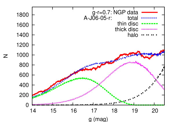
In figure 6 the contributions of thin disc, thick disc, and stellar halo for model A are shown in the colour bin as a typical example. The maximum contribution of the thin disc is at mag corresponding to pc and of the thick disc at mag corresponding to pc. These large distances demonstrate that it is very important to construct models, which hold also for the outer profiles of the components.
Model A-J06-05-r is the best model with a reduced (see table 1). In model A the deviations of data and model are less than percent over the full colour range and in the magnitude regime, where the MS stars of thin disc, thick disc or halo dominate. The distribution in figure 5 shows a strong noise component and the contribution by systematic deviations of the predicted density profiles from the real profiles. In the top panel of figure 7 the reduced values in each colour bin are quantified. The contributions to the total are fairly uniform.
The main feature of the systematic discrepancies is the shallow valley in the transition of thin disc and thick disc in the data, which is not reproduced by the model. This is a sign of an even steeper slope of the thin disc above 1 kpc. A continuous transition between the old thin disc with a maximum vertical velocity dispersion of km/s and the thick disc with km/s can be excluded, because it would add more stars to the transition regime.
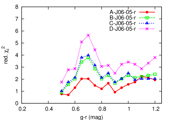
In models B, C, and D, the fits in the magnitude range of dominating thin disc contribution are significantly worse, whereas the thick disc parameters can be adjusted to reach a similar good fit at fainter magnitudes as in model A. This is also quantified in the values (see table 1). Model D with the small disc age and strongly declining SFR is the worst model with . Models B and C are comparable with and 3.84, respectively. All three models overestimate the thin disc density at large heights leading to a deficit closer to the plane. A more detailed look on the distributions shows that model A is superior in a wide colour range (figure 7).
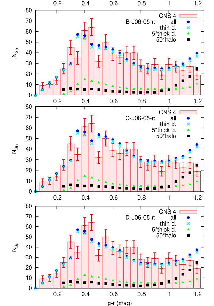
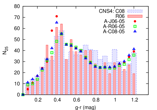
Since we used the local number densities of all components as free fitting parameters, a comparison of the fitting results and the observed star counts in the solar neighbourhood is a crucial test of the models. In figure 8 the histogram with error-bars shows the data from the CNS4. The full (blue) circles are the results of model A – D (from top to bottom). In all cases there is a reasonable match and also the total number of MS stars agree (see table 1). The observed number of MS stars range from (with R06) to (with C08). Additionally the contribution of thin disc, thick disc and halo is plotted separately in figure 8 (enhanced by some factor to make it visible) demonstrating that the local number densities of all components are smooth functions of . A more detailed discussion is given in section 6.3.
As a bottom line we find that the local disc model A is fully consistent with the NGP star count data of SDSS. Model A with a relatively large fraction of stars older than 8 Gyr and a correspondingly small maximum vertical velocity dispersion of km/s is the best fitting model. In the next sub-sections we test the robustness of the result with respect to the filter transformations used for the solar neighbourhood and with respect to the smoothing in .
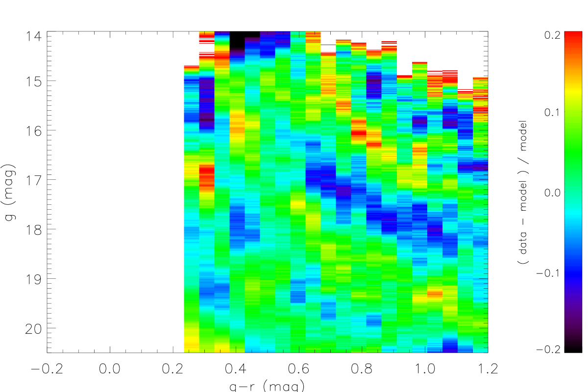
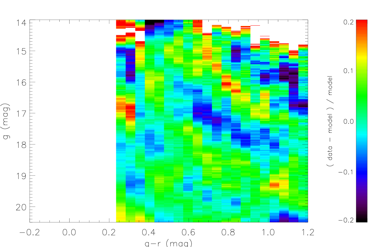
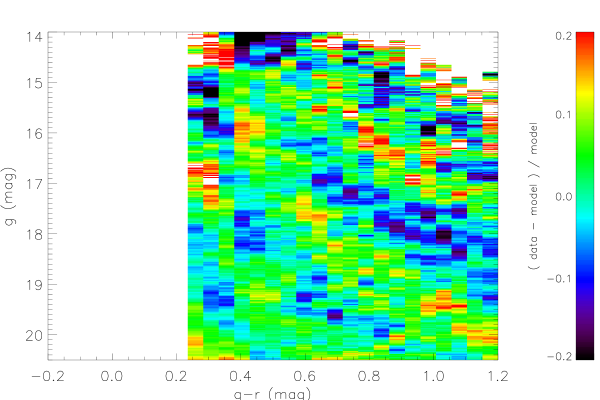
6.3 Filter transformations
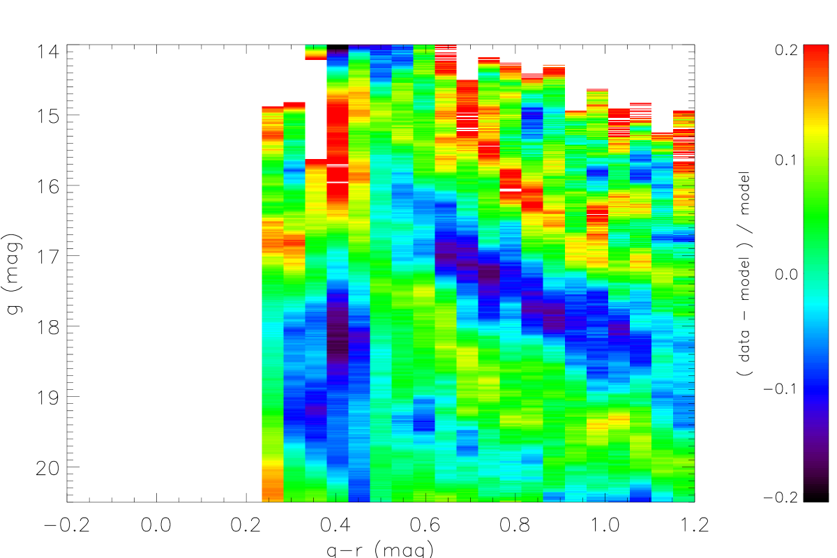
In figure 9 the local MS is shown for three different transformations (J06 for Jordi et al. (2006), R06 for Rodgers et al. (2006), C08 for Chonis & Gaskell (2008)). There are small systematic deviations in which may influence the best fit parameters of the model. The histograms in figure 11 show the local star counts for R06 and C08. Additionally to the differences in the absolute magnitudes for thin and thick disc the fraction of thin disc turn-off stars is reduced in C08 and is set to zero in R06 in order to test their influence on the values and number counts.
We present the comparison using the different local MS for model A. The effects in models B, C and D are very similar. First we derived the best fit models for the reduced colour-magnitude regime as before in A-J06-05-r for models A-R06-05-r and A-C08-05-r (see table 1). The total values and local normalisations of the three models are very similar.
Then we extended the fit regime to the full CMD and recalculated the local normalisations and the values.
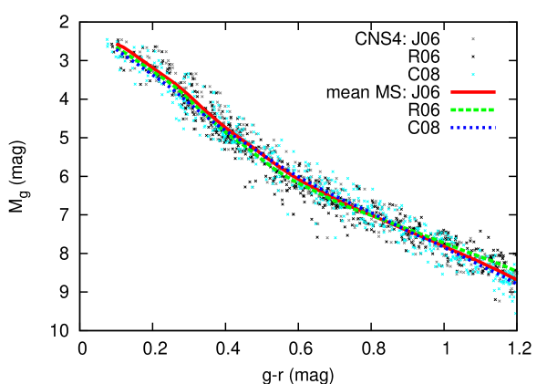
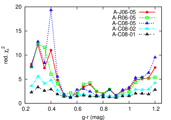
Figure 10 shows the relative deviations of data and models. The patterns of the deviations differ slightly in the regime, where the thin disc dominates. The corresponding values in the colour bins are shown in the lower panel of figure 7. For the extended fit regime there are small differences arising mainly from the turn-off stars. In the colour bin the fraction of turn-off stars is 80 percent (J06), 0 percent (R06) and 60 percent (C08), respectively. Model A-R06-05 without turn-off stars gives the best result. A consequence is that a larger fraction of stars are allocated to the thick disc instead of the thin disc in model A-R06-05 (see figure 11). At model A-J06-05 with 55 percent turn-off stars gives the best result and for the turn-off stars are too bright to contribute to the fit. At the red end is influenced by the missing giants. Therefore it is not useful to discuss here the differences of the fits in more detail.

The local normalisations do not differ significantly (see figure 11). The differences in the histograms for the transformations R06 and C08 show the possible variations in the local star counts due to noise and the effect of a different slope in the MS leading to a shift of stars in colour. All transformations are consistent with the local star count data. Only in the transition of K to M dwarfs the large number of thin disc stars in may be a hint that the MS turning point is relatively blue as in C08.
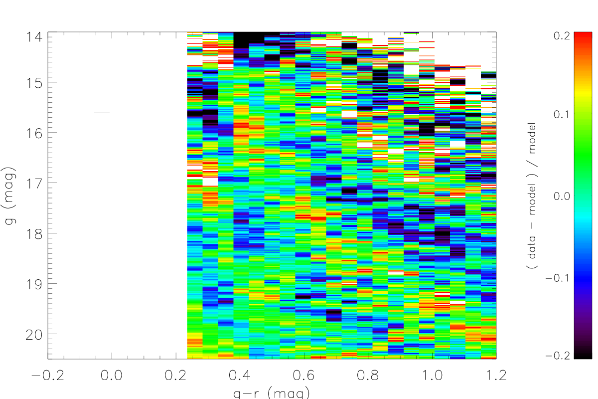
6.4 Smoothing
Smoothing of the data has two main effects. On one hand statistical noise is reduced. On the other hand physical features in the data are smeared out and may be shifted systematically. Figure 12 shows the NGP data and corresponding models A-C08-05,02,01 for different smoothing lengths 0.5, 0.2, 0.1 mag, respectively. The values are decreasing due to to the increasing degrees of freedom (see table 1 and figure 7). The local normalisations are statistically indistinguishable. Only in the colour bin a few percent of thin disc stars are shifted to the thick disc at higher resolution reducing the contribution to by the bright magnitude bins dramatically.
7 Conclusions
We have used four different models with different SFRs of the thin disc, which fit the local kinematics of main sequence (MS) stars (Paper I) and compared the star count predictions for the North Galactic Pole (NGP) field with of the Sloan Digital Sky Survey (SDSS). For the thin disc we applied the absolute magnitudes of the local MS as determined in Just & Jahreiss (2008). A self-consistent isothermal thick disc and a simple stellar halo model was added to complete the contributions of MS stars to the star counts. We used the local normalisations of thin disc, thick disc and halo in each colour bin as free parameters and minimise in the Hess diagram over a large colour-magnitude range in .
All models match the observed number densities better than percent proving the reliability of the thin disc density profiles by the self-consistent disc models in the range of kpc. The derived local normalisations are consistent with the star count data of the CNS4 in the solar neighbourhood. The analysis shows that model A is clearly preferred with systematic deviations of a few percent only. The SFR of model A is characterised by a maximum at an age of 10 Gyr and a decline by a factor of four to the present day value of 1.4 /pc2/Gyr. In the thin disc the present day fraction of stars older than 8 Gyr is with 54 percent significantly higher than for models B, C, and D (Paper I). Especially model C with a constant SFR and model D with a disc age of 10 Gyr can be ruled out.
The thick disc can be modelled very well by an isothermal simple stellar population. The density profile can be approximated by a sech function. For model A we find a power law index of in-between an exponential profile and a sech2-profile (the latter corresponds to an isolated isothermal disc). The exponential scale height is pc corresponding to a vertical velocity dispersion of km/s. About 6 percent of the stars in the solar neighbourhood are thick disc stars. In Jurić et al. (2008) the stellar density distribution in the Milky Way based on SDSS star counts was fitted by exponential thin and thick disc profiles. The result is a much larger thick disc scale height, which balances the flattening of the profile at low .
The results do not depend significantly on the filter transformations used for the local MS nor on the smoothing of the data in luminosity. For the future an extension of the model to include turn-off stars in more detail and the contribution of giants as well as a higher resolution in colour at the blue end would be very useful.
We also plan to apply the model to lower Galactic latitudes in order to determine radial scale lengths of thin and thick disc as well as radial gradients in the stellar populations.
Acknowledgements
SG is supported by a grant of the Chinese Academy of Science.
SV was supported by an Alexander von Humboldt Fellowship (Web Site http://www.humboldt-foundation.de).
Funding for the SDSS and SDSS-II has been provided by the Alfred P. Sloan Foundation, the Participating Institutions, the National Science Foundation, the U.S. Department of Energy, the National Aeronautics and Space Administration, the Japanese Monbukagakusho, the Max Planck Society, and the Higher Education Funding Council for England. The SDSS Web Site is http://www.sdss.org/.
The SDSS is managed by the Astrophysical Research Consortium for the Participating Institutions. The Participating Institutions are the American Museum of Natural History, Astrophysical Institute Potsdam, University of Basel, University of Cambridge, Case Western Reserve University, University of Chicago, Drexel University, Fermilab, the Institute for Advanced Study, the Japan Participation Group, Johns Hopkins University, the Joint Institute for Nuclear Astrophysics, the Kavli Institute for Particle Astrophysics and Cosmology, the Korean Scientist Group, the Chinese Academy of Sciences (LAMOST), Los Alamos National Laboratory, the Max-Planck-Institute for Astronomy (MPIA), the Max-Planck-Institute for Astrophysics (MPA), New Mexico State University, Ohio State University, University of Pittsburgh, University of Portsmouth, Princeton University, the United States Naval Observatory, and the University of Washington.


References
- Abazajian et al. (2003) Abazajian, K. N., et al. 2003, AJ, 126, 2081
- Abazajian et al. (2004) Abazajian, K. N., et al. 2004, AJ, 128, 502
- Abazajian et al. (2009) Abazajian, K. N., et al. 2009, ApJS, 182, 543
- Adelman-McCarthy et al. (2008) Adelman-McCarthy, J. K., et al. 2008, ApJS, 175, 297
- An et al. (2008) An, D., et al. 2008, ApJS, 179, 326
- Bilir et al. (2008) Bilir, S., Ak, S., Karaali, S., Cabrera-Lavers, A., Chonis, T. S., & Gaskell, C. M. 2008, MNRAS, 384, 1178
- Chonis & Gaskell (2008) Chonis, T. S., & Gaskell, C. M. 2008, AJ, 135, 264
- Fukugita et al. (1996) Fukugita, M., Ichikawa, T., Gunn, J. E., Doi, M., Shimasaku, K., & Schneider, D. P. 1996, AJ, 111, 1748
- Gunn et al. (1998) Gunn, J. E. et al. 1998, AJ, 116, 3040
- Gunn et al. (2006) Gunn, J. E. et al. 2006, AJ, 131, 2332
- Hogg et al. (2001) Hogg, D.W., Finkbeiner, D.P., Schlegel, D.J., Gunn, J.E. 2001, AJ, 122, 2129
- Ivezić et al. (2003) Ivezić, Ž., et al. 2003, Proceedings of the Workshop Variability with Wide Field Imagers, Mem. Soc. Ast. It., 74, 978 (also astro-ph/0301400)
- Ivezić et al. (2004) Ivezić, Ž. et al. 2004, AN, 325, 583
- Ivezić et al. (2008) Ivezić, Ž. et al. 2008, ApJ, 684, 287
- Jahreiß & Wielen (1997) Jahreiß H., Wielen R. 1997, In B. Battrick, M. A. C. Perryman, eds., Proc. ESA SP-402 (Nordwijk, ESA), 675
- Jordi et al. (2006) Jordi, K., Grebel, E. K., & Ammon, K. 2006, A&A, 460, 339
- Jurić et al. (2008) Jurić, M., et al. 2008, ApJ, 673, 864
- Just & Jahreiss (2008) Just, A., Jahreiss, H. 2008, AN, 329, 790
- Just & Jahreiss (2010) Just, A., Jahreiss, H. 2010, MNRAS, 402, 461
- Landolt (1992) Landolt, A. U. 1992, AJ, 104, 340
- Lupton, Gunn, & Szalay (1999) Lupton, R., Gunn, J., & Szalay, A. 1999, AJ, 118, 1406
- Lupton et al. (2001) Lupton R. H., Gunn J. E., Ivezić Ž., Knapp G. R., Kent S., 2001, in ASP Conf. Ser. 238, Astronomical Data Analysis Software and Systems X., ed. F. R. Harnden Jr., F. A. Primini & H. E. Payne (San Francisco: ASP), 269
- Padmanabhan, N., et al. (2008) Padmanabhan, N., et al., 2008, ApJ, 674, 1217
- Pier et al. (2003) Pier, J. R., Munn, J. A., Hindsley, R. B, Hennessy, G. S., Kent, S. M., Lupton, R. H., Ivezić, Ž. 2003, AJ, 125, 1559
- Press et al. (1992) Press W. H., Teukolsky S. A., Vetterling W. T., Flannery B. P. (eds.), Numerical Recipes, Cambridge Univ. Press, Cambridge, 1992
- Rodgers et al. (2006) Rodgers, C. T., Canterna, R., Smith, J. A., Pierce, M. J., & Tucker, D. L. 2006, AJ, 132, 989
- Schlegel et al. (1998) Schlegel, D. J., Finkbeiner, D. P., & Davis, M. 1998, ApJ, 500, 525
- Smith et al. (2002) Smith, J. A., et al. 2002, AJ, 123, 2121
- Stoughton et al. (2002) Stoughton, C. et al. 2002, AJ, 123, 485
- Tucker et al. (2006) Tucker, D. L., et al. 2006, AN, 327, 821
- York et al. (2000) York D.G., et al. 2000, AJ, 120, 1579