Directed excitation transfer in vibrating chains by external fields

Abstract

We study the coherent dynamics of excitations on vibrating chains. By applying an external field and matching the field strength with the oscillation frequency of the chain it is possible to obtain an (average) transport of an initial Gaussian wave packet. We distinguish between a uniform oscillation of all nodes of the chain and the chain being in its lowest eigenmode. Both cases can lead to directed transport.

I Introduction

The transport of energy or charge is fundamental for a large variety of physical, chemical, and biological processes. One of the most prominent examples is the energy transfer in the light-harvesting complexes in photosynthesis Fleming and Scholes (2004). There, the energy of the captured solar photons is transported via a molecular backbone to the reaction center where the energy is transformed into chemical energy. Recent experiments have shown that coherent features of the transport process might be crucial for a high efficiency Engel et al. (2007); Collini et al. (2010). Usually, the system and the dynamics of the excitation (exciton) is modeled by open quantum systems where the system of interest, e.g., the light-harvesting complex, is coupled to an external environment. It has been shown that the environment can also support the coherent dynamics Cheng and Silbey (2006); Mohseni et al. (2008); Caruso et al. (2009); Olaya-Castro et al. (2008); Thorwart et al. (2009); Mülken and Schmid (2010).

Most of the models assume a time-independent Hamiltonian motivated by the fact that, indeed, the network of chromophores underlying the energy transfer is rather static, even at higher (room) temperatures. However, this need not be the case. One can easily imagine the situation where the underlying molecule is not static but performs some kind of mechanical oscillation. Asadian et al. have shown that certain types of motions can enhance the transfer efficiency when compared to the static situation Asadian et al. (2010). In a related model, Semião et al. studied the modulation of the excitation energies of coupled quantum dots driven by a nanomechanical resonator mode, also enhancing the transport efficiency Semião et al. (2010). Vaziri and Plenio showed that the periodic modulation of ion channels leads to the emergence of resonances in their transport efficiency Vaziri and Plenio (2010).

Another influence on the dynamics can be external fields. Hartmann et al. have shown for the coherent transport of an initial Gaussian wave packet on a discrete (static) chain of nodes that by suitably switching the direction of a constant external field, one can achieve directed transport Hartmann et al. (2004). There, the switching frequency has been matched with the Bloch oscillation frequency. The effect of Bloch oscillations on the trapping of excitations has been studied by Vlaming et al., finding that the trapping efficiency crucially depends on the strength of the external field (the bias) Vlaming et al. (2007, 2008).

Clearly, mechanical motions and external fields are not restricted to energy transfer in molecular aggregates. Other examples include cold atoms in optical lattices whose spacings can be periodically modulated Al-Assam et al. (2010) or waveguide arrays where the “external field” is achieved by a linear variation of the effective refractive index across the array, see, e.g., Christodoulides et al. (2003).

A question we address in this paper is whether it is possible to engineer the excitation transport in systems performing mechanical oscillations with a constant external field such that also here one obtains directed transport.

II Model

We consider the excitation dynamics on a finite chain of $N$ nodes with time-dependent couplings $J_{n}(t)$ between two adjacent nodes of the chain. The Hamiltonian in the node-basis $\{|n\rangle,n=1..N\}$ reads

$$\bm{H}_{0}=\sum_{n=1}^{N}E_{n}|n\rangle\langle n|+\sum_{n=1}^{N-1}J_{n}(t)\big{(}|n\rangle\langle n+1|+|n+1\rangle\langle n|\big{)},$$ (1)

where the $E_{n}$ are the site energies. Now, in addtion we apply an external field with strength $f$, such that the total Hamiltonian for an excitation on a vibrating chain reads

$$\bm{H}_{S}=\bm{H}_{0}+f\sum_{n=1}^{N}n|n\rangle\langle n|.$$ (2)

For chains whose nodes (molecules or atoms) interact via dipole-dipole forces, the couplings decay with the third power of the distance between the nodes. For fairly large distances between adjacent nodes the coupling to next-nearest neighbors can be neglected such that the assumption of nearest neigbor couplings in $H_{0}$ can be justified.

Now, there are two competing effects: On the one hand excitations in a static chain with an external field perform Bloch oscillations Hartmann et al. (2004); Holthaus and Hone (1996); Fukuyama et al. (1973). On the other hand the time-dependent couplings can cause an enhanced transport efficiency Asadian et al. (2010); Semião et al. (2010); Vaziri and Plenio (2010). If the oscillations are periodic, the distances between two adjacent nodes vary in a given interval. Short distances means stronger couplings and thus faster transport from node to node. Longer distances lead to weaker couplings and slower transport. Therefore, matching the Bloch frequency with the frequency of the chain oscillation should lead to an effective transport in one direction along the chain. The reason is that in the first half of the Bloch period $T_{B}$ the distances between the nodes are smaller while in the second half of $T_{B}$ the distances are larger. This leads to different displacements in the two half periods and consequently to an overall displacement of the inital excitation in one direction.

We choose two scenarios for the couplings $J_{n}(t)$:

(i) Each node of the chain oscillates uniformly with the same frequency $\omega$ and with the the same amplitude $a$. The couplings follow now as

$$J_{n}(t)=J(t)=-V/\Big{[}1-2a\sin(\omega t+\phi)\Big{]}^{3}.$$ (3)

The same setting has been used by Asadian et al Asadian et al. (2010). In the following we also assume all site-energies to be the same, i.e., we set $E_{n}=E=0$.

(ii) The chain is in its lowest eigenmode, such that for the $q$th eigenmode the couplings $J_{n,q}(t)$ between $n$th and $(n+1)$st node are

$$J_{n,q}(t)=-V/\Big{[}1-2a_{n,q}\sin(\omega_{q}t+\phi)\Big{]}^{3},$$ (4)

see Sec. III.3 for details.

Clearly, for time-constant $J_{n}=J$ we recover the known Bloch oscillations with frequency $\omega_{B}=f/\hbar$ (we set $\hbar=1$ in the following). Thus, the period of the oscillation $T_{B}=2\pi/\omega_{B}=2\pi/f$.

The dynamics of an initial excitation is governed by the Liouville-von Neumann equation for the density operator $\bm{\rho}(t)$. Without any external environment leading to decoherence, the dynamics is fully coherent following

$$\dot{\bm{\rho}}(t)=-i[\bm{H}_{S},\bm{\rho}(t)].$$ (5)

Now, if the system is coupled to an environment such that the total Hamiltonian can be split into three parts, $\bm{H}_{\rm tot}=\bm{H}_{S}+\bm{H}_{R}+\bm{H}_{RS}$, where $H_{R}$ is the Hamiltonian of the environment and $H_{RS}$ is the Hamiltonian of the system-environmental coupling. For small couplings to the environment we will study the dynamics by the Lindblad quantum master equation Breuer and Petruccione (2006)

$$\dot{\bm{\rho}}(t)=-i[\bm{H}_{S},\bm{\rho}(t)]-\lambda\sum_{j=1}^{N}\big{(}\bm{\rho}(t)-\langle j|\bm{\rho}(t)|j\rangle\big{)}|j\rangle\langle j|,$$ (6)

where we assumed Lindblad operators of the form $\sqrt{\lambda}|j\rangle\langle j|$. The term proportional to $\lambda$ mimicks the influence of the environment leading to decoherence. In the following we will consider the occupation probabilities $\rho_{kk}(t)\equiv\langle k|\bm{\rho}(t)|k\rangle$ for a given initial condition $\bm{\rho}(0)$.

III Results

In all calculations shown below we used $N=103$ and an initial Gaussian wave packet centered at $N_{c}(0)=N_{0}$ with a standard deviation of $\sigma=6$. We adjust $N_{0}$ such that in the first two periods of the Bloch oscillations the wave packet does not encounter the edges of the chain, such that we can exclude interference effects caused by reflection. We further take $V=1$.

III.1 Static chain

We start by considering the static chain, i.e., no oscillations ($a=0$). Without any external field and no external environment, the dynamics of wave packets on the static chain is very similar to the motion of a quantum particle in a box Mülken and Blumen (2005, 2006). One can also observe (partial) revivals of initially localized wave packets caused by reflections at the end of the chain, thus obtaining the discrete analog of so-called quantum carpets Kinzel (1995); Grossmann et al. (1997).

When applying an external field, the situation changes. Figure 1 shows for $N_{0}=78$ the well-known Bloch oscillations in the occupation probabilities $\rho_{kk}(t)$ with Bloch frequency $\omega_{B}=f$ for $f=0.2$ with no external coupling, $\lambda=0$, (left panel) and with small external coupling, $\lambda=0.05$, (right panel). One clearly recognizes the oscillation period of $T_{B}=2\pi/f=10\pi$. The coupling to the environment leads to a spreading of the wave packet over more and more nodes as time progresses. Eventually, this will lead to the equilibium distribution.

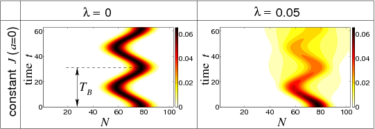
Figure 1: (Color online) Static chain: Contour plot of the occupation probabilities for $a=0$ and $f=0.2$ with $\lambda=0$ (left panel) and $\lambda=0.05$ (right panel). Dark (black) regions correspond to large probabilities, while bright (yellow/white) regions correspond to low probabilities.

In a continuous approximation for an infinite line, the position of the center of the wave packet follows for vanishing initial momentum as Hartmann et al. (2004); Holthaus and Hone (1996); Fukuyama et al. (1973)

$$\Delta N(t)\equiv N_{c}(t)-N_{0}\simeq-\frac{4V}{f}\sin^{2}(ft/2).$$ (7)

Obviously, there is no transport after integer values of $T_{B}$, only after $T_{B}/2=\pi/f$ has the wave packet travelled by $|\Delta N(T_{B}/2)|=4V/f=20$ nodes in the direction of the field. We note that by instantly reversing the field after $T_{B}/2$ the wave packet will continue to move to the left side, such that it is possible to obtain directed transport by switching the field every half-period, see Hartmann et al. (2004) for details.

III.2 Uniformly oscillating chain

If the chain is not static ($a\neq 0$) but oscillates such that the couplings are given by Eq. (3), it is possible to obtain - on average - a net transport of the wave packet in one direction. However, this will depend on the choice of the field strength $f$, i.e., on the frequency of the Bloch oscillation, on the phase shift $\phi$, and on the amplitude $a$.

III.2.1 Analytical approximation

Before turning to the numerical results, we give an analytical estimate of the displacements $\Delta N_{l}\equiv[N_{c}(lT_{B})-N_{0}]$ ($l\in\mathbb{N}$) of the center of the wave packet after integer values of the Bloch period $T_{B}$. For the static (infinite) chain, starting from Eq. (7) and differentiating with respect to time, one has

$$\dot{N}(t)=-4V\sin(ft/2)\cos(ft/2)=-2V\sin(ft),$$ (8)

which gives the temporal change of the displacement. Thus, the rate of transport from node to node is $V$. We extend this idea to the oscillating chain and replace the coupling $V$ with the time-dependent coupling $J(t)$. Then, we define the approximate displacements by integrating $\dot{N}(t)$ over integer values of $T_{B}$:

$$\Delta N_{l,{\rm approx}}\equiv-2V\int\limits_{0}^{lT_{B}}dt\ \frac{\sin(ft)}{\big{[}1-2a\sin(\omega t+\phi)\big{]}^{3}}.$$ (9)

For $\omega=f$ this leads to

$$\Delta N_{l,{\rm approx}}=-\frac{12l\pi aV\cos\phi}{f(1-4a^{2})^{5/2}}.$$ (10)

Clearly, the displacement is maximal for $\phi=0$ and minimal (zero) for $\phi=\pi$. Note that $\Delta N_{l,{\rm approx}}$ is only valid for the infinite chain. In the following we will compare $\Delta N_{l,{\rm approx}}$ to numerical results obtained from Eq. (6). As we will show, for the uniformly oscillating chain, $\Delta N_{l,{\rm approx}}$ agrees very well with the numerical results. Also for the chain in its lowest eigenmode we will use $\Delta N_{l,{\rm approx}}$ as a starting point to define an adhoc fitting function $\Delta N_{l,{\rm fit}}$ which also turns out to be in very good agreement with the numerical results.

III.2.2 Numerical results

Figure 2 shows the occupation probabilities $\rho_{kk}(t)$ for the case $\omega_{B}=f=\omega=0.2$ with $a=0.1$ and for different phase shifts $\phi$. Again, the left panels show the results for isolated chains ($\lambda=0$) and the right panels for small couplings to an external environment ($\lambda=0.05$). Plots in different rows correspond to different $\phi$. Matching $f$ with $\omega$ and having no phase shift results - on average - in a directed transport of the initial wave packet in the direction of the field. In the second half of each Bloch period $T_{B}$ the wave packet moves in the opposite direction. However, this is overcompensated by the motion in the direction of the field in the first half of each period.

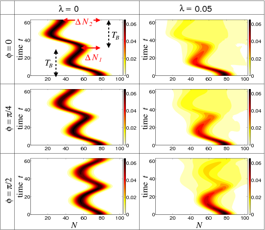
Figure 2: (Color online) Oscillating chain: Contour plot of the occupation probabilities $\rho_{kk}(t)$ for $a=0.1$ and $\omega=f=0.2$ with $\lambda=0$ (left panels) and $\lambda=0.05$ (right panels). The three rows correspond to different values of $\phi=0,\pi/4$ and $\pi/2$, respectively.

The dependence on the phase shift can be expressed by only considering the average displacement $\Delta N_{l}$. Figure 3 shows the dependence of $\Delta N_{1}$ and $\Delta N_{2}/2$ on $\phi$ for the same parameters as in Fig. 2, but with $N_{0}=52$. Changing the initial condition to the center of the chain allows to vary $\phi$ in between $0$ and $2\pi$ and thus avoiding interference effects due to reflections at the ends of the chain. Note that this has no influence on the dynamics because the couplings in the chain are translational invariant. We distinguish between $\Delta N_{1}$ after one and $\Delta N_{2}$ after two periods because, in general, one cannot expect a linear behavior of $\Delta N_{l}$ in $l$. However, as it turns out $\Delta N_{l}$ is approximately linear in $l$ for the uniformly oscillating chain.

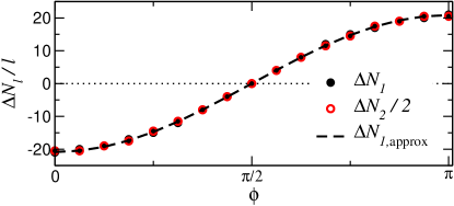
Figure 3: (Color online) Oscillating chain: Displacements $\Delta N_{l}/l$ with $l=1,2$, extracted from the occupation probabilities for $N_{0}=52$, as a function of $\phi$ for $a=0.1$, $\omega=f=0.2$ and $\lambda=0$. The dashed lines show $\Delta N_{l,{\rm approx}}$ given in Eq. (9).

Changing the phase shift allows to control the transport: No phase shift ($\phi=0$) results in values of $\Delta N_{1}\approx-21$ after one period. A phase shift of $\phi=\pi/2$ results in a behavior similar to the Bloch oscillations in the static chain, i.e., no transport, see also Fig. 1. Increasing $\phi$ further leads to a reversed motion, i.e., the wave packet moves “uphill” against the direction of the field. For $\phi=\pi$ the maximal displacement after one period of $\Delta N_{1}\approx 21$ is obtained. For the uniformly oscillating chain, the values for $\Delta N_{2}/2$ coincide with the ones for $\Delta N_{1}$ leading to the linear behavior $\Delta N_{l}=l\Delta N_{1}$. In addition, Fig. 3 shows the analytical estimate of Eq. (9) which agrees with the numerical results.

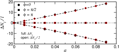
Figure 4: (Color online) Oscillating chain: Displacements $\Delta N_{l}/l$ with $l=1,2$ as a function of $a$ for $N_{0}=52$, $\omega=f=0.2$, $\phi=0,\pi/2,\pi$ and $\lambda=0$. The dashed lines show $\Delta N_{l,{\rm approx}}$ given in Eq. (9).

The magnitude of the displacements $\Delta N_{l}$ also depends on $a$. Figure 4 shows $\Delta N_{l}/l$ as a function of $a$ for $N_{0}=52$ and $\phi=0,\pi/2$, and $\pi$. While for $\phi=\pi/2$ there is no displacement after integer values of $T_{B}$, the displacements for $\phi=0$ and for $\phi=\pi$ grow with increasing $a$. Again, the dashed lines show the approximation $\Delta N_{1,{\rm approx}}$ which nicely agrees with the numerical results.

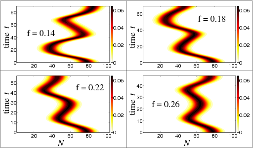
Figure 5: (Color online) Oscillating chain: Contour plot of the occupation probabilities $\rho_{kk}(t)$ with $\omega=0.2$, $a=0.1$, $\phi=0$, and $\lambda=0$ for different values of $f$.

The effect of having directed transport depends on having the field strength in resonance with the chain oscillation frequency. In order to see how crucial the exact matching of $f$ and $\omega$ is, we study slightly detuned frequencies $\omega_{B}$, i.e., a mismatch between $\omega$ and $f$. Figure 5 shows for $\phi=0$ (leading to maximal $\Delta N_{l}$ for $\omega=f$) and for $\omega=0.2$ the occupation probabilities $\rho_{kk}(t)$ for different values of $f$. Note that changing $f$ also changes the Bloch period $T_{B}=2\pi/f$, thus the time axes are different for different $f$. A field strength of $f=0.18$ or $f=0.22$ reflects a detuning by $\pm 10\%$ of $\omega$. This still results in an average directed transport after two periods of $\Delta N_{2}\approx 30$ for $f=0.18$ and of $\Delta N_{2}\approx 36$ for $f=0.22$. Increasing the detuning further diminishes the transport.

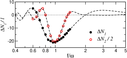
Figure 6: (Color online) Oscillating chain: Displacements $\Delta N_{l}/l$ with $l=1,2$ as a function of $f$ for $a=0.1$, $\omega=0.2$, $\phi=0$, and $\lambda=0$ (note the semi-logarithmic scale). The dashed lines show the approximation obtained by numerical integration, see text for details.

Figure 6 shows the displacements $\Delta N_{l}/l$ for $\phi=0$ and different values of $f$. The maximal displacement is obtained for $\omega\approx f$, as expected. Decreasing or increasing $f$ results in smaller displacements: For $f>\omega$ the decrease in displacement is slower than for $f<\omega$. One also observes that the displacements change directions. For $f<\omega$, $\Delta N_{2}/2$ changes direction at about $f/\omega=0.8$ and $\Delta N_{1}$ at about $f/\omega\approx 0.67$. For $f>\omega$, the direction change happens at larger deviations from the resonace condition. Additionally, there are maximal displacements in the opposite direction.

As before, we can obtain an approximation to the numerical results: Considering now $f\neq\omega$ in Eq. (9) and numerically integrating over integer values of the Bloch oscillation yields the dashed curves shown in Fig. 6. Again, the approximation is in very good agreement with the numerical data.

Having now explored a large region of the parameters $f/\omega$, $a$, and $\phi$, we see that the dynamics of an initial Gaussian wave packet can be manipulated by a suitable choice of these parameters: We can make the wave packet move - on average - in one preferred direction by choosing the phase shift $\phi$. The magnitude of the displacements in either direction is given by $a$. Moreover, we do not have to exactly match the Bloch frequency $\omega_{B}=f$ with the oscillation frequency $\omega$ in order to obtain directed transport, there is a fairly large range of roughly $\pm 10\%$ around $f/\omega=1$ in which large displacements can be obtained.

III.3 Chain in lowest eigenmode

In contrast to the previous section, we now consider the dynamics on a finite chain in its lowest eigenmode. Although this mode is similar to the uniform oscillation, the finite size of the chain becomes crucial leading to a non-uniform oscillation of the nodes.

The couplings $J_{n,q}(t)$ in Eq. (4) between the nodes are obtained from a normal mode analysis of a free chain of nodes connected by springs, see Asadian et al. (2010) for details. Although the motion of the nodes is not uniform Rosenstock (1955), there are close similarities to the results presented in the previous section.

In order to obtain comparable results we have to adjust the amplitudes and frequencies according to the couplings $J_{n,q}(t)$ between nodes $n$ and $n+1$ for the $q$th eigenmode. The couplings in Eq. (4) can be written as

$$J_{n,q}(t) = -V\Bigg{[}1-\frac{2a\sin[2\omega t\sin(q\pi/2N)+\phi]}{\cos(q\pi/2N)}$$ (11)

$$\times\sin(nq\pi/N)\sin(q\pi/2N)\Bigg{]}^{-3},$$

such that one has

$$a_{n,q}\equiv\frac{a\sin(nq\pi/N)\sin(q\pi/2N)}{\cos(q\pi/2N)}$$ (12)

and

$$\omega_{q}\equiv 2\omega\sin(q\pi/2N).$$ (13)

Thus, in the following we will use $\omega_{q}=f$ as the resonance condition for the frequency and the field. For the amplitude $a_{n,q}$ to be comparable to the amplitudes in the previous section, we consider the average absolute value of the amplitudes, i.e.,

$$\bar{a}_{q} \equiv \frac{1}{N}\sum_{n=1}^{N}|a_{n,q}|=\frac{a}{N}\tan(q\pi/2N)\sum_{n=1}^{N}|\sin(nq\pi/N)|$$ (14)

$$= \frac{aq}{N}\tan(q\pi/2N)\cot(q\pi/2N)=\frac{aq}{N}.$$

Thus, we consider amplitudes $\bar{a}_{q}$ which - on average - are of the same order as the ones in the previous section. This means that we choose the parameter $a$ in Eq. (12) to be $a=N\bar{a}_{q}/q$.

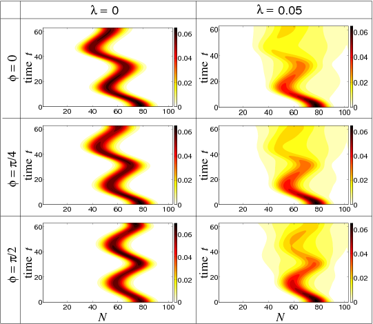
Figure 7: (Color online) Lowest eigenmode: Contour plot of the occupation probabilities $\rho_{kk}(t)$ for $\bar{a}_{1}=0.04$ and $\omega_{1}=f=0.2$ with $\lambda=0$ (left panels) and $\lambda=0.05$ (right panels). The three rows correspond to different values of $\phi=0,\pi/4$ and $\pi/2$, respectively.

Similarly to Fig. 2, Fig. 7 shows the occupation probabilities $\rho_{kk}(t)$ for the case $\omega_{B}=f=\omega_{1}$. All plots in Fig. 7 show results for $\bar{a}_{1}=0.04$. We use $\bar{a}_{1}=0.04$ because this clearly avoids interference effects due to reflections at the ends of the chain. Coupling this system to an external environment leads, again, to decoherence and a spreading of the initial wave packet.

Figure 8 shows a comparison of the displacements $\Delta N_{l}$ as a function of the phase shift $\phi$ for different $N_{0}$. Already for the central initial node, $N_{0}=52$ (upper panel), one notices the asymmetry between the behavior of $\Delta N_{1}$ and $\Delta N_{2}/2$ for values of $\phi\in[0,\pi/2]$ and values of $\phi\in[\pi/2,\pi]$. For $\phi>\pi$ the difference between $\Delta N_{1}$ and $\Delta N_{2}/2$ is smaller than for $\phi<\pi/2$, see in particular the points for $\phi=0$ and $\phi=\pi$. One also notices that $\phi=\pi/2$ yields $\Delta N_{l}\neq 0$, in contrast to the uniformly oscillating chain. However, the overall behaviors for the two chains are very similar. Therefore, we fit our numerical result for $\Delta N_{1}$ by a cosine, as suggested by Eq. (9), namely, we use

$$\Delta N_{l,{\rm fit}}\equiv\beta_{l}\frac{\bar{a}_{1}\cos(\phi+\alpha_{l})}{(1-4\bar{a}_{1}^{2})^{5/2}},$$ (15)

where $\alpha_{l}$ and $\beta_{l}$ are ($l$-dependent) fit parameters. This already yields a very good agreement with the numerical results, see the dashed lines in Fig. 8.

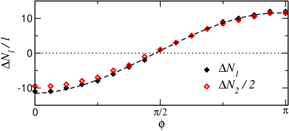
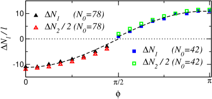
Figure 8: (Color online) Lowest eigenmode: Displacements $\Delta N_{l}/l$ with $l=1,2$ for $N_{0}=52$ (upper panel) and for $N_{0}=42$ and $N_{0}=78$ (lower panel) as a function of $\phi$ for $\bar{a}_{1}=0.04$, $\omega_{1}=f=0.2$, and $\lambda=0$. The dashed lines show the fits for $\Delta N_{l,{\rm fit}}$ given by Eq. (15).

Changing the initial node $N_{0}$ influences the behavior of the wave packet. Figure 8 also shows the behavior of $\Delta N_{1}$ and $\Delta N_{2}/2$ for $N_{0}=42$ (lower panel, right half) and $N_{0}=78$ (lower panel, left half). While for $N_{0}=52$ one has $|\Delta N_{1}|\geq|\Delta N_{2}/2|$, one observes for $N=42$ and for $N_{0}=78$ that $|\Delta N_{1}|\leq|\Delta N_{2}/2|$. However, for all initial nodes shown in Fig. 8, the maximal displacements (for $\phi=0$ and $\phi=\pi$) are in the same region about $|\Delta N_{l}/l|\approx 12$.

The slight asymmetry can be attributed to the non-uniform, i.e., non-translational invariant, motion of the nodes of the chain and the additional influence of the external field, which breaks the point symmetry with respect to the center.

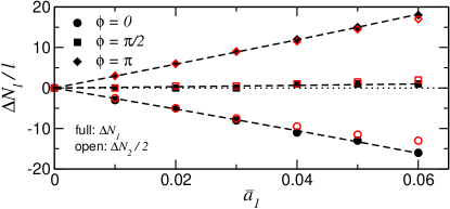
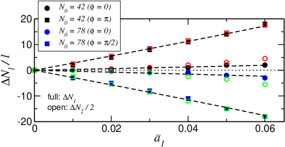
Figure 9: (Color online) Lowest eigenmode: Displacements $\Delta N_{l}/l$ with $l=1,2$ as a function of $\bar{a}_{1}$ for $\omega_{1}=f=0.2$, and $\lambda=0$: upper panel for $N_{0}=52$ with $\phi=0,\pi/2,\pi$ and lower panel for $N_{0}=42$ with $\phi=\pi/2,\pi$ and $N_{0}=78$ with $\phi=0,\pi/2$. The dashed lines show the fits for $\Delta N_{1,{\rm fit}}$ given by Eq. (15).

The $\bar{a}_{1}$-dependence of the displacements is shown in Fig. 9. Although the absolute values of $\Delta N_{l}/l$ are different for different $N_{0}$, there is a similar behavior for different values of $\phi$. Moreover, the behavior is similar to the one for the uniformly oscillating chain, see Fig. 4. Therefore, we fit the $\bar{a}_{1}$-dependence of $\Delta N_{1}$ by $\Delta N_{1,{\rm fit}}$ given in Eq. (15). Also here are the fits in very good agreement with the numerical results.

Figure 10 shows the displacements $\Delta N_{1}$ and $\Delta N_{2}/2$ as a function of $f$ for $\phi=0$. Similar to the oscillating chain, the displacements are maximal for $f\approx\omega_{1}$. The dashed lines show the approximations obtained for the oscillating chain (see Fig. 6) but rescaled by a factor $1/2$. Already this rough approximation yields good agreement to the numerical results. However, the points for $f/\omega=0.6$ have to be considered with care, because such a detuning leads to interference effects due to reflection at the end node of the chain after one half period. This interference obviously can influence the dynamics of the wave packet.

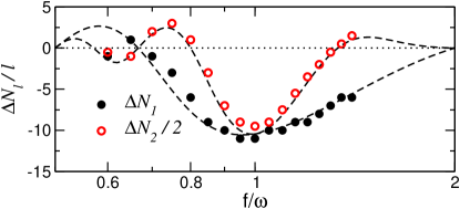
Figure 10: (Color online) Lowest eigenmode: Displacements $\Delta N_{l}/l$ with $l=1,2$ as a function of $f$ for $\bar{a}_{1}=0.04$, $\omega_{1}=0.2$, $\phi=0$, and $\lambda=0$ (note the semi-logarithmic scale). The dashed lines show the approximations of Fig. 6 scaled by a factor of $1/2$, see text for details.

Now, also for the chain in its lowest eigenmode we obtain similar results to the ones for the oscillating chain. However, the absolute values of the parameters are different. Nevertheless, the approximations given by Eq. (9) turn out to give qualitatively the correct behavior. Therefore, the same conclusions as for the oscillating chain apply here.

IV Conclusions

We have studied the coherent transport of excitations on a finite chain with time-dependent couplings between adjacent nodes of the chain and in the presence of an external field. The field leads to Bloch oscillations while regular time-dependent couplings can lead to an increased transport efficiency of excitations along the chain. We showed for uniformly oscillating chains and for a chain in its lowest eigenmode that matching the Bloch oscillation frequency with the frequency of the chain leads to an (average) directed displacement of an initial Gaussian wave packet. Applying a phase difference allows to manipulate the direction of the transport, while changing the amplitude of the regular oscillation allows to manipulate the strength of the displacements. We corroborate our findings by an analytic (continuous) approximation for the average displacement of an initial Gaussian wave packet in an infinite chain after integer values of the Bloch period. For the uniformly oscillating chain, this ansatz yields a functional form for the displacements, which agrees very well with the numerical data. Using the same functional form also allows to define a fitting function for the chain in its lowest eigenmode, also leading to very good agreement with the numerical results. In both cases, interference effects due to reflections at the ends of the chains have been neglected.